Statistical inference using Regularized M-estimation in the reproducing kernel Hilbert space for handling missing data

Abstract

Imputation and propensity score weighting are two popular techniques for handling missing data. We address these problems using the regularized M-estimation techniques in the reproducing kernel Hilbert space. Specifically, we first use the kernel ridge regression to develop imputation for handling item nonresponse. While this nonparametric approach is potentially promising for imputation, its statistical properties are not investigated in the literature. Under some conditions on the order of the tuning parameter, we first establish the root-$n$ consistency of the kernel ridge regression imputation estimator and show that it achieves the lower bound of the semiparametric asymptotic variance. A nonparametric propensity score estimator using the reproducing kernel Hilbert space is also developed by a novel application of the maximum entropy method for the density ratio function estimation. We show that the resulting propensity score estimator is asymptotically equivalent to the kernel ridge regression imputation estimator. Results from a limited simulation study are also presented to confirm our theory. The proposed method is applied to analyze the air pollution data measured in Beijing, China.

Keywords: Imputation; Kernel ridge regression; Missing at random; Propensity score.

1 Introduction

Missing data is a universal problem in statistics. Ignoring the cases with missing values can lead to misleading results (Kim and Shao, 2013; Little and Rubin, 2019). Two popular approaches for handling missing data are imputation and propensity score weighting. Both approaches are based on some assumptions about the data structure and the response mechanism. To avoid potential biases due to model misspecification, instead of using strong parametric model assumptions, nonparametric approaches are preferred as they do not depend on explicit model assumptions.

In principle, any prediction techniques can be used to impute for missing values using the responding units as a training sample. However, statistical inference with imputed estimator is not straightforward. Treating imputed data as if observed and applying the standard estimation procedure may result in misleading inference, leading to underestimation of the variance of imputed point estimators. How to incorporate the uncertainty of the estimated parameters in the final inference is challenging especially for nonparametric imputation because the model parameter is implicitly defined.

For nonparametric imputation, Cheng (1994) used the kernel-based nonparametric regression for imputation and established the root-$n$ consistency of the imputed estimator. Chen and Shao (2001) considered nearest neighbor imputation and discuss its variance estimation. Wang and Chen (2009) employed the kernel smoothing approach to do empirical likelihood inference with missing values. Yang and Kim (2020) considered predictive mean matching imputation and established its asymptotic properties. Kim et al. (2014) proposed Bayesian multiple imputation using the Dirichlet process mixture. Sang et al. (2020) proposed semiparametric fractional imputation using Gaussian mixtures.

For nonparametric propensity score estimation, Hainmueller (2012) proposed so-called the entropy balancing method to find the propensity score weights using the Kullback-Leibler information criterion with finite-dimensional basis function. Chen et al. (2013) established the root-${n}$ consistency of the kernel-based nonparametric propensity score estimator. Chan et al. (2016) generalized the entropy balancing method of Hainmueller (2012) further to develop a general calibration weighting method that satisfies the covariance balancing property with increasing dimensions of the control variables. They further showed the global efficiency of the proposed calibration weighting estimator. Zhao (2019) generalized the idea further and developed a unified approach of covariate balancing propensity score method using tailored loss functions. Tan (2020) developed regularized calibrated estimation of propensity scores with high dimensional covariates. While nonparametric kernel regression can be used to construct nonparametric propensity score estimation, as in Chen et al. (2013), it is not clear how to generalize it to a wider function space to obtain nonparametric propensity score estimation.

In this paper, we consider regularized M-estimation as a tool for nonparametric function estimation for imputation and propensity score estimation. Kernel ridge regression (Friedman et al., 2001; Shawe-Taylor et al., 2004) is an example of the regularized M-estimation for a modern regression technique. By using a regularized M-estimator in reproducing kernel Hilbert space (RKHS), kernel ridge regression can estimate the regression mean function with complex reproducing kernel Hilbert space while a regularized term makes the original infinite dimensional estimation problem viable (Wahba, 1990). Due to its flexibility in the choice of kernel functions, kernel ridge regression is very popular in machine learning. van de Geer (2000); Mendelson (2002); Zhang (2005); Koltchinskii et al. (2006); Steinwart et al. (2009) studied the error bounds for the estimates of kernel ridge regression method.

While the kernel ridge regression is a promising tool for handling missing data, its statistical inference is not investigated in the literature. We aim to fill in this important research gap in the missing data literature by establishing the statistical properties of the KRR imputation estimator. Specifically, we obtain root-$n$ consistency of the KRR imputation estimator under some popular functional Hilbert spaces. Because the KRR is a general tool for nonparametric regression with flexible assumptions, the proposed imputation method can be used widely to handle missing data without employing parameteric model assumptions. Variance estimation after the kernel ridge regression imputation is a challenging but important problem. To the best of our knowledge, this is the first paper which considers kernel ridge regression technique for imputation and discusses its variance estimation rigorously.

The regularized M-estimation technique in RKHS is also used to obtain nonparametric propensity score weights for handling missing data. To do this, we use a novel application of density ratio function estimation in the same reproducing kernel Hilbert space. Maximum entropy method of Nguyen et al. (2010) for density ratio estimation is adopted to get the nonparametric propensity score estimators. We further show the asymptotic equivalence of the resulting propensity score estimator with the kernel ridge regression-based imputation estimator. These theoretical findings can be used to make valid statistical inferences with the propensity score estimator.

The paper is organized as follows. In Section 2, the basic setup and the KRR method is introduced. In Section 3, the root-$n$ consistency of the KRR imputation estimator is established. In Section 4, we introduce a novel nonparametric propensity score estimator using the regularized M-estimation technique in the RKHS. Results from a limited simulation study are presented in Section 5. An illustration of the proposed method to a real data example is presented in Section 6. Some concluding remarks are made in Section 7.

2 Basic setup

Consider the problem of estimating $\theta=E(Y)$ from an independent and identically distributed sample $\{(\boldsymbol{x}_{i},y_{i}),i=1,\cdots,n\}$ of random vector $(\boldsymbol{X},Y)$. Instead of always observing $y_{i}$, suppose that we observe $y_{i}$ only if $\delta_{i}=1$, where $\delta_{i}$ is the response indicator function of unit $i$ taking values on $\{0,1\}$. The auxiliary variable $\boldsymbol{x}_{i}$ are always observed. We assume that the response mechanism is missing at random (MAR) in the sense of Rubin (1976).

Under MAR, we can develop a nonparametric estimator $\hat{m}(\boldsymbol{x})$ of $m(\boldsymbol{x})=E(Y\mid\boldsymbol{x})$ and construct the following imputation estimator:

$$\hat{\theta}_{I}=\frac{1}{n}\sum_{i=1}^{n}\left\{\delta_{i}y_{i}+(1-\delta_{i})\hat{m}(\boldsymbol{x}_{i})\right\}.$$ (1)

If $\hat{m}(\boldsymbol{x})$ is constructed by the kernel-based nonparametric regression method, we can express

$$\hat{m}(\boldsymbol{x})=\frac{\sum_{i=1}^{n}\delta_{i}K_{h}(\boldsymbol{x}_{i},\boldsymbol{x})y_{i}}{\sum_{i=1}^{n}\delta_{i}K_{h}(\boldsymbol{x}_{i},\boldsymbol{x})}$$ (2)

where $K_{h}(\cdot)$ is the kernel function with bandwidth $h$. Under some suitable choice of the bandwidth $h$, Cheng (1994) first established the root-$n$ consistency of the imputation estimator (1) with nonparametric function in (2). However, the kernel-based regression imputation in (2) is applicable only when the dimension of $\boldsymbol{x}$ is small.

In this paper, we extend the work of Cheng (1994) by considering a more general type of the nonparametric imputation, called kernel ridge regression imputation. The kernel ridge regression (KRR) can be understood using the reproducing kernel Hilbert space theory (Aronszajn, 1950) and can be described as

$$\hat{m}=\operatorname*{arg\,min}_{m\in\mathcal{H}}\left[\sum_{i=1}^{n}\delta_{i}\left\{y_{i}-m(\boldsymbol{x}_{i})\right\}^{2}+\lambda\left\|m\right\|_{\mathcal{H}}^{2}\right],$$ (3)

where $\left\|m\right\|_{\mathcal{H}}^{2}$ is the norm of $m$ in the reproducing kernel Hilbert space $\mathcal{H}$ and $\lambda(>0)$ is a tuning parameter for regularization. Here, the inner product $\langle\cdot,\cdot\rangle_{\mathcal{H}}$ is induced by such a kernel function, i.e.,

$$\langle f,K(\cdot,\boldsymbol{x})\rangle_{\mathcal{H}}=f(\boldsymbol{x}),$$

for any $\boldsymbol{x}\in\mathcal{X},f\in\mathcal{H}$, namely, the reproducing property of $\mathcal{H}$. Naturally, this reproducing property implies the $\mathcal{H}$ norm of $f$: $\left\|f\right\|_{\mathcal{H}}=\langle f,f\rangle_{\mathcal{H}}^{1/2}$. Scholkopf and Smola (2002) provides a comprehensive overview of the machine learning techniques using the reproducing kernel functions.

One canonical example of such a functional Hilbert space is the Sobolev space. Specifically, assuming that the domain of such functional space is $[0,1]$, the Sobolev space of order $\ell$ can be denoted as

$$\mathcal{W}_{2}^{\ell} = \left\{f:[0,1]\rightarrow\mathbb{R}\mid f,f^{(1)},\dots,f^{(\ell-1)}\subset\mathbb{C}[0,1],\quad f^{(\ell)}\in L^{2}[0,1]\right\},$$

where $\mathbb{C}[0,1]$ denotes the absolutely continuous function on $[0,1]$. One possible norm for this space can be

$$\left\|f\right\|_{\mathcal{W}_{2}^{\ell}}^{2}=\sum_{q=0}^{\ell-1}\left\{\int_{0}^{1}f^{(q)}(t)dt\right\}^{2}+\int_{0}^{1}\left\{f^{(\ell)}(t)\right\}^{2}dt.$$

In this section, we employ the Sobolev space of second order as the approximation function space. For Sobolev space of order $\ell$, we have the kernel function

$$K(x,y)=\sum_{q=0}^{\ell-1}k_{q}(x)k_{q}(y)+k_{\ell}(x)k_{\ell}(y)+(-1)^{\ell}k_{2\ell}(|x-y|),$$

where $k_{q}(x)=(q!)^{-1}B_{q}(x)$ and $B_{q}(\cdot)$ is the Bernoulli polynomial of order $q$. Smoothing spline method is a special case of the kernel ridge regression method.

By the representer theorem for reproducing kernel Hilbert space (Wahba, 1990), the estimate in (3) lies in the linear span of $\{K(\cdot,\boldsymbol{x}_{i}),i=1,\ldots,n\}$. Specifically, we have

$$\hat{m}(\cdot)=\sum_{i=1}^{n}\hat{\alpha}_{i,\lambda}K(\cdot,\boldsymbol{x}_{i}),$$ (4)

where

$$\hat{\boldsymbol{\alpha}}_{\lambda}=\left(\boldsymbol{\Delta}_{n}\mathbf{K}+\lambda\boldsymbol{I}_{n}\right)^{-1}\boldsymbol{\Delta}_{n}\boldsymbol{y},$$

$\boldsymbol{\Delta}_{n}=\mbox{diag}(\delta_{1},\ldots,\delta_{n})$, $\mathbf{K}=(K(\boldsymbol{x}_{i},\boldsymbol{x}_{j}))_{ij}$, $\boldsymbol{y}=(y_{1},\ldots,y_{n})^{\rm T}$ and $\boldsymbol{I}_{n}$ is the $n\times n$ identity matrix.

The tuning parameter $\lambda$ is selected via generalized cross-validation in kernel ridge regeression, where the criterion for $\lambda$ is

$$\mbox{GCV}(\lambda)=\frac{n^{-1}\left\|\left\{\boldsymbol{\Delta}_{n}-\boldsymbol{A}(\lambda)\right\}\boldsymbol{y}\right\|_{2}^{2}}{n^{-1}{\rm{tr}}(\boldsymbol{\Delta}_{n}-\boldsymbol{A}(\lambda))},$$ (5)

and $\boldsymbol{A}(\lambda)=\boldsymbol{\Delta}_{n}\mathbf{K}(\boldsymbol{\Delta}_{n}\mathbf{K}+\lambda\boldsymbol{I}_{n})^{-1}\boldsymbol{\Delta}_{n}$. The value of $\lambda$ minimizing the criterion (5) is used for the selected tuning parameter.

Using the kernel ridge regression (KRR) imputation in (3), we can obtain the imputed estimator in (1). Because $\hat{m}(\boldsymbol{x})$ in (4) is a nonparametric regression estimator of $m(\boldsymbol{x})=E(Y\mid\boldsymbol{x})$, we can expect that this imputation estimator in (1) is consistent for $\theta=E(Y)$ under missing at random, as long as $\hat{m}(\boldsymbol{x})$ is a consistent estimator of $m(\boldsymbol{x})$. Surprisingly, it turns out that the consistency of $\hat{\theta}_{I}$ to $\theta$ is of order $O_{p}(n^{-1/2})$, while the point-wise convergence rate for $\hat{m}(\boldsymbol{x})$ to $m(\boldsymbol{x})$ is slower. This is consistent with the theory of Cheng (1994) for kernel-based nonparametric regression imputation.

We aim to establish two goals: (i) find the sufficient conditions for the root-$n$ consistency of the KRR imputation estimator and give a formal proof; (ii) find a linearization variance formula for the KRR imputation estimator. The first part is formally presented in Theorem 1 in Section 3. For the second part, we employ the density ratio estimation method of Nguyen et al. (2010) to get a consistent estimator of $\omega(\boldsymbol{x})=\{\pi(\boldsymbol{x})\}^{-1}$ in the linearized version of $\hat{\theta}_{I}$. Estimation of $\omega(\boldsymbol{x})$ will be presented in Section 4.

3 Main Theory

Before we develop our main theory, we first introduce Mercer’s theorem.

Lemma 1 (Mercer’s theorem)

Given a continuous, symmetric, positive definite kernel function $K:\mathcal{X}\times\mathcal{X}\mapsto\mathbb{R}$. For $\boldsymbol{x},\boldsymbol{z}\in\mathcal{X}$, under some regularity conditions, Mercer’s theorem characterizes $K$ by the following expansion

$$K(\boldsymbol{x},\boldsymbol{z})=\sum_{j=1}^{\infty}\lambda_{j}\psi_{j}(\boldsymbol{x})\psi_{j}(\boldsymbol{z}),$$

where $\lambda_{1}\geq\lambda_{2}\geq\ldots\geq 0$ are a non-negative sequence of eigenvalues, $\{\psi_{j}\}_{j=1}^{\infty}$ is an orthonormal basis for $L^{2}(\mathbb{P})$ and $\mathbb{P}$ is the given distribution of $\boldsymbol{X}$ on $\mathcal{X}$.

Furthermore, we make the following assumptions.

[A1] For some $k\geq 2$, there is a constant $\rho<\infty$ such that $E[\psi_{j}(X)^{2k}]\leq\rho^{2k}$ for all $j\in\mathbb{N}$, where $\{\psi_{j}\}_{j=1}^{\infty}$ are orthonormal basis by expansion from Mercer’s theorem.

[A2] The function $m\in\mathcal{H}$, and for $\boldsymbol{x}\in\mathcal{X}$, we have $E[\left\{Y-m(\boldsymbol{x})\right\}^{2}\mid\boldsymbol{x}]\leq\sigma^{2}$, for some $\sigma^{2}<\infty$.

[A3] The response mechanism is missing at random. Furthermore, the propensity score $\pi(\boldsymbol{x})=P(\delta=1\mid\boldsymbol{x})$ is uniformly bounded away from zero. In particular, there exists a positive constant $c>0$ such that $\pi(\boldsymbol{x}_{i})\geq c$, for $i=1,\ldots,n$.

The first assumption is a technical assumption which controls the tail behavior of $\{\psi_{j}\}_{j=1}^{\infty}$. Assumption 3 indicates that the noises have bounded variance. Assumption 3 and Assumption 3 together aim to control the error bound of the kernel ridge regression estimate $\hat{m}$. Furthermore, Assumption 3 means that the support for the respondents should be the same as the original sample support. Assumption 3 is a standard assumption for missing data analysis.

We further introduce the following lemma. Let $\boldsymbol{S}_{\lambda}=(\boldsymbol{I}_{n}+\lambda\mathbf{K}^{-1})^{-1}$ be the linear smoother for the KRR method. That is, $\hat{m}=\boldsymbol{S}_{\lambda}\boldsymbol{y}$ be the vector of regression predictor of $\boldsymbol{y}$ using the kernel ridge regression method. We now present the following lemma without proof which is modified from Lemma 7 in Zhang et al. (2013).

Lemma 2

Under [A1]-[A2], for a random vector $\boldsymbol{z}=E(\boldsymbol{z})+\sigma\boldsymbol{\varepsilon}$, we have

$$\boldsymbol{S}_{\lambda}\boldsymbol{z}=E(\boldsymbol{z}\mid\boldsymbol{x})+\boldsymbol{a}_{n},$$

where $\boldsymbol{a}_{n}=(a_{1},\ldots,a_{n})^{\rm T}$ and

$$a_{i}=\mathcal{O}_{p}\left(\lambda^{1/2}+\{\gamma(\lambda)\}^{1/2}n^{-1/2}\right),$$ (6)

for $i=1,\ldots,n$, as long as $E(\left\|z_{i}\right\|_{\mathcal{H}})$ and $\sigma^{2}$ is bounded from above, for $i=1,\ldots,n$, where $\boldsymbol{\varepsilon}=(\boldsymbol{\varepsilon}_{1},\cdots,\boldsymbol{\varepsilon}_{n})^{\rm T}$ are noise vector with mean zero and bounded variance and

$$\gamma(\lambda)=\sum_{j=1}^{\infty}\frac{\mu_{j}}{\mu_{j}+\lambda},$$

is the effective dimension and $\{\mu_{j}\}_{j=1}^{\infty}$ are the eigenvalues of kernel $K$ used in $\hat{m}(\boldsymbol{x})$.

The first term in (6) denotes the order of bias term and the second term denotes the square root of the variance term. Specifically, we have the asymptotic mean square error for $\hat{m}$,

$$\mbox{AMSE}(\hat{m})=O(1)\times\left\{\lambda\left\|m\right\|_{\mathcal{H}}^{2}+n^{-1}\gamma(\lambda)\right\}.$$ (7)

For the $\ell$-th order of Sobolev space, we have $\mu_{j}\leq Cj^{-2\ell}$ and

$$\gamma({\lambda})=\sum_{j=1}^{\infty}(1+j^{2\ell}{\lambda})^{-1}\leq O\left(\lambda^{-1/(2\ell)}\right).$$ (8)

Note that (7) is minimized when $\lambda\asymp\gamma(\lambda)/n,$ which is equivalent to ${\lambda}\asymp n^{-2\ell/(2\ell+1)}$ under (8). The optimal rate $\lambda\asymp n^{-2\ell/(2\ell+1)}$ leads to

$$\mbox{AMSE}(\hat{m})=O(n^{-2\ell/(2\ell+1)})$$ (9)

which is the optimal rate in Sobolev space, as discussed by Stone (1982).

To investigate the asymptotic properties of the kernel ridge regression imputation estimator, we express

$$\hat{\theta}_{I} =\frac{1}{n}\sum_{i=1}^{n}\left\{\delta_{i}y_{i}+(1-\delta_{i})\hat{m}(\boldsymbol{x}_{i})\right\}$$

$$=\underbrace{\frac{1}{n}\sum_{i=1}^{n}m(\boldsymbol{x}_{i})}_{R_{n}}+\underbrace{\frac{1}{n}\sum_{i=1}^{n}\delta_{i}\left\{y_{i}-m(\boldsymbol{x}_{i})\right\}}_{S_{n}}+\underbrace{\frac{1}{n}\sum_{i=1}^{n}(1-\delta_{i})\left\{\hat{m}(\boldsymbol{x}_{i})-m(\boldsymbol{x}_{i})\right\}}_{T_{n}}.$$

Therefore, as long as we show

$$T_{n}=\frac{1}{n}\sum_{i=1}^{n}\delta_{i}\left\{\frac{1}{\pi(\boldsymbol{x}_{i})}-1\right\}\left\{y_{i}-m(\boldsymbol{x}_{i})\right\}+o_{p}(n^{-1/2}),$$ (10)

then we can establish the root-$n$ consistency. The following theorem formally states the theoretical result. A proof of Theorem 1 is presented in the supplementary material.

Theorem 1

Suppose Assumption 3-3 hold for a Sobolev kernel of order $\ell$, as long as

$$n\lambda\rightarrow 0,\quad n\lambda^{1/2\ell}\rightarrow\infty,$$ (11)

we have

$$n^{1/2}\left(\hat{\theta}_{I}-\theta\right){\rightarrow}N(0,\sigma^{2}),$$

where

$$\sigma^{2}=\mbox{Var}\{E(Y\mid\boldsymbol{x})\}+E\{\mbox{Var}(Y\mid\boldsymbol{x})/\pi(\boldsymbol{x})\}=\mbox{Var}(\eta)$$

with

$$\eta =m(\boldsymbol{x})+\delta\frac{1}{\pi(\boldsymbol{x})}\left\{y-m(\boldsymbol{x})\right\}.$$ (12)

Remark 1

Note that the optimal rate ${\lambda}\asymp n^{-2\ell/(2\ell+1)}$ does not satisfy the first part of (11). To control the bias part, we need a smaller $\lambda$ such as $\lambda=n^{-\kappa}$ with $\kappa>1$. Similar conditions are used for bandwidth selection for nonparametric kernel regression with bandwidth $h$:

$$nh\rightarrow\infty\mbox{ and }n^{1/2}h^{2}\rightarrow 0$$

for $\mbox{dim}(\boldsymbol{x})=1$. See Wang and Chen (2009) for details.

Remark 2

Theorem 1 is presented for a Sololev kernel, and any kernel whose eigenvalues have the same tail behavior as Sobolev of order $\ell$ also has the result as Theorem 1. For sub-Gaussian kernel whose eigenvalues satisfy that

$$\mu_{j}\leq c_{1}\exp(-c_{2}j^{2}),$$

where $c_{1},c_{2}$ are positive constants, we can establish similar results. To see this, note that

$$\gamma(\lambda) =\sum_{j=1}^{\infty}\frac{\mu_{j}}{\mu_{j}+\lambda}$$

$$\leq c_{2}^{-1/2}\{-\log(\lambda)\}^{1/2}+\frac{1}{\lambda}\int_{c_{2}^{-1/2}\{-\log(\lambda)\}^{1/2}}\exp(-c_{2}z^{2})dz$$

$$\leq c_{2}^{-1/2}\{-\log(\lambda)\}^{1/2}+O(1),$$

where the second term in the last equation can be obtained by the Gaussian tail bound inequality. Therefore, as long as $n\lambda\rightarrow 0$ and $n\{-\log(\lambda)\}^{-1/2}\rightarrow\infty$, we have $n^{-1}\boldsymbol{1}_{n}^{\rm T}\boldsymbol{a}=o_{p}(n^{-1/2})$ and the root-$n$ consistency can be established.

Note that the asymptotic variance of the imputation estimator is equal to $n^{-1}\sigma^{2}$, which is the lower bound of the semiparametric asymptotic variance discussed in Robins et al. (1994). Thus, the kernel ridge regression imputation is asymptotically optimal. The main term (12) in the linearization in Theorem 1 is called the influence function (Hampel, 1974). The term influence function is motivated by the fact that to the first order $\eta_{i}=m(\boldsymbol{x}_{i})+\delta_{i}\{\pi(\boldsymbol{x}_{i})\}^{-1}\left\{y_{i}-m(\boldsymbol{x}_{i})\right\}$ is the influence of a single observation on the estimator $\hat{\theta}_{I}$.

The influence function in (12) can be used for variance estimation of the KRR imputation estimator $\hat{\theta}_{I}$. The idea is to estimate the influence function $\eta_{i}=m(\boldsymbol{x}_{i})+\delta_{i}\{\pi(\boldsymbol{x}_{i})\}^{-1}\left\{y_{i}-m(\boldsymbol{x}_{i})\right\}$ and apply the standard variance estimator using $\hat{\eta}_{i}$. To estimate $\eta_{i}$, we need an estimator of $\pi(\boldsymbol{x})$. In the next section, we will consider a version of kernel ridge regression to estimate $\omega(x)=\{\pi(\boldsymbol{x})\}^{-1}$ directly. Once $\hat{\omega}_{i}(\boldsymbol{x})$ is obtained, we can use

$$\hat{\mbox{V}}=\frac{1}{n}\frac{1}{n-1}\sum_{i=1}^{n}\left(\hat{\eta}_{i}-\bar{\eta}_{n}\right)^{2}$$

as a variance estimator of $\hat{\theta}_{I}$ in (1), where

$$\hat{\eta}_{i}=\hat{m}(\boldsymbol{x}_{i})+\delta_{i}\hat{\omega}_{i}(\boldsymbol{x}_{i})\left\{y_{i}-\hat{m}(\boldsymbol{x}_{i})\right\}$$

and $\bar{\eta}_{n}=n^{-1}\sum_{i=1}^{n}\hat{\eta}_{i}$.

4 Propensity score estimation

We now consider estimation of the propensity weight function $\omega(x)=\{\pi(\boldsymbol{x})\}^{-1}$ using kernel ridge regression. In order to estimate $\omega(\boldsymbol{x})=\{\pi(\boldsymbol{x})\}^{-1}$, we wish to develop a nonparametric method of estimating $\omega(\boldsymbol{x})$ using the same RKHS theory. To do this, we use the density ratio function estimation approach to propensity score function estimation proposed by Wang and Kim (2021). To introduce the idea, we first define the following density ratio function

$$g(\boldsymbol{x})=\frac{f(\boldsymbol{x}\mid\delta=0)}{f(\boldsymbol{x}\mid\delta=1)},$$ (13)

and, by Bayes theorem, we have

$$\omega(\boldsymbol{x})=\frac{1}{\pi(\boldsymbol{x})}=1+c\cdot g(\boldsymbol{x})$$

where $c=P(\delta=0)/P(\delta=1)$. Thus, to estimate $\omega(\boldsymbol{x})$, we have only to estimate the density ration function $g(\boldsymbol{x})$ in (13). Now, to estimate $g(\boldsymbol{x})$, we use the maximum entropy method (Nguyen et al., 2010) for density ratio function estimation. Kanamori et al. (2012) also considered the M-estimator of the density ratio function with the Kullback-Leibler divergence.

For convenience, let $f_{k}(\boldsymbol{x})=f(\boldsymbol{x}\mid\delta=k)$, for $k=0,1$. To explain the M-estimation of $g(\boldsymbol{x})$, note that $g(\boldsymbol{x})$ can be understood as the maximizer of the objective function on the right-hand-side of (14) which is upper bounded by the Kullback-Leibler divergence between $f_{0}$ and $f_{1}$, i.e.,

$$D_{KL}(f_{0},f_{1}) =\max_{g>0}Q(g)+1$$

$$=\max_{g>0}\int\log\left\{g(\boldsymbol{x})\right\}f_{0}(\boldsymbol{x})d\mu(\boldsymbol{x})-\int g(x)f_{1}(\boldsymbol{x})d\mu(x)+1$$

$$=\max_{g>0}\int g(\boldsymbol{x})[\log\left\{g(\boldsymbol{x})\right\}-1]f_{1}(\boldsymbol{x})d\mu(\boldsymbol{x})+1.$$ (14)

That is, by (14), a sample version of $Q(g)$ can be written as

$$\hat{Q}(g)=\frac{1}{n_{1}}\sum_{i=1}^{n}\delta_{i}g(\boldsymbol{x}_{i})[\log\{g(\boldsymbol{x}_{i})\}-1],$$

where $n_{1}=\sum_{i=1}^{n}\delta_{i}$.

Since $g(\boldsymbol{x})$ is unknown, we want to impose constraints to formulate an M-estimation problem for $g(\boldsymbol{x})$. Given $\hat{m}(\cdot)$, using the idea of model calibration (Wu and Sitter, 2001), we would like to use

$$\frac{1}{n_{1}}\sum_{i=1}^{n}\delta_{i}g(\boldsymbol{x}_{i})\hat{m}(\boldsymbol{x}_{i})=\frac{1}{n_{0}}\sum_{i=1}^{n}(1-\delta_{i})\hat{m}(\boldsymbol{x}_{i})$$

as a constraint for density ratio estimation, where $n_{0}=n-n_{1}$. Note that it is algebraically equivalent to

$$\frac{1}{n}\sum_{i=1}^{n}\delta_{i}\left\{1+\frac{n_{0}}{n_{1}}\cdot{g}(\boldsymbol{x}_{i})\right\}\hat{m}(\boldsymbol{x}_{i})=\frac{1}{n}\sum_{i=1}^{n}\hat{m}(\boldsymbol{x}_{i}).$$

Now, as we have $m\in\mathcal{H}$, and by the representer theorem in kernel ridge regression, we know that $\hat{m}\in\mbox{span}\{K(\cdot,\boldsymbol{x}_{1}),\ldots,K(\cdot,\boldsymbol{x}_{n})\}$. Thus, the calibration constraint is

$$\frac{1}{n_{1}}\sum_{i=1}^{n}\delta_{i}g(\boldsymbol{x}_{i})(K(\cdot,\boldsymbol{x}_{1}),\ldots,K(\cdot,\boldsymbol{x}_{n}))^{\rm T}=\frac{1}{n_{0}}\sum_{i=1}^{n}(1-\delta_{i})(K(\cdot,\boldsymbol{x}_{1}),\ldots,K(\cdot,\boldsymbol{x}_{n}))^{\rm T}.$$ (15)

This calibration property is also called covariate-balancing property (Imai and Ratkovic, 2014). Further, we want to incorporate with the normalization constraint $\sum_{i=1}^{n}\delta_{i}\omega(\boldsymbol{x}_{i})=n$, i.e.,

$$\frac{1}{n_{1}}\sum_{i=1}^{n}\delta_{i}g(\boldsymbol{x}_{i})=\frac{1}{n_{0}}\sum_{i=1}^{n}(1-\delta_{i}).$$ (16)

Minimizing $\hat{Q}(g)$ subject to (15) and (16) is called the maximum entropy method. Using Lagrangian multiplier method, the solution to this optimization problem can be written as

$$\log\{g(\boldsymbol{x})\}\equiv\log\{g(\boldsymbol{x};\boldsymbol{\phi})\}=\phi_{0}+\sum_{i=1}^{n}\phi_{i}K(\boldsymbol{x},\boldsymbol{x}_{i})$$ (17)

for some $\boldsymbol{\phi}=(\phi_{0},\ldots,\phi_{n})^{\rm T}\in\mathbb{R}^{n+1}$. Thus, using the parametric form in (17), the optimization problem can be expressed as a dual form

$$\hat{Q}_{0}(\boldsymbol{\phi})=\frac{1}{n_{0}}\sum_{i=1}^{n}(1-\delta_{i})\log\{g(\boldsymbol{x}_{i};\boldsymbol{\phi})\}-\frac{1}{n_{1}}\sum_{i=1}^{n}\delta_{i}g(\boldsymbol{x}_{i};\boldsymbol{\phi}),$$

to formulate a legitimate estimation of $g(\cdot)$. Further, define $h(\boldsymbol{x};\boldsymbol{\phi}_{s})=\log\{g(\boldsymbol{x};\boldsymbol{\phi})\}-\phi_{0}$, where $\boldsymbol{\phi}_{s}=(\phi_{1},\ldots,\phi_{n})^{\rm T}$. In our problem, to ensure the Representer theorem, we wish to find $h$ that minimizes

$$-\hat{Q}_{0}(g;\boldsymbol{\phi})+\tau\left\|h\right\|_{\mathcal{H}}^{2}$$ (18)

over $\boldsymbol{\phi}$.

Hence, the solution to (18) can be obtained as

$$\min_{\boldsymbol{\phi}_{s}\in\mathbb{R}^{n}}\left\{\frac{1}{n_{1}}\sum_{i=1}^{n}\delta_{i}g(\boldsymbol{x}_{i};\boldsymbol{\phi})-\frac{1}{n_{0}}\sum_{i=1}^{n}(1-\delta_{i})\log\{g(\boldsymbol{x}_{i};\boldsymbol{\phi})\}+\tau\boldsymbol{\phi}^{\rm T}\mathbf{K}\boldsymbol{\phi}\right\}$$ (19)

and $\phi_{0}$ is a normalizing constant satisfying

$$n_{1}=\sum_{i=1}^{n}\delta_{i}\exp\{\phi_{0}+\sum_{j=1}^{n}\hat{\phi}_{j}K(\boldsymbol{x}_{i},\boldsymbol{x}_{j})\}.$$ (20)

Thus, we use

$$\hat{g}(x)=\exp\{\hat{\phi}_{0}+\sum_{j=1}^{n}\hat{\phi}_{j}K(\boldsymbol{x},\boldsymbol{x}_{j})\}$$

as the maximum entropy estimator of the density ratio function $g(\boldsymbol{x})$ using kernel method. Also,

$$\hat{\omega}(\boldsymbol{x})=1+\frac{n_{0}}{n_{1}}\hat{g}(\boldsymbol{x})$$

is the maximum entropy estimator of $\omega(x)=\{\pi(\boldsymbol{x})\}^{-1}$. The estimator of $\omega(x)$ satisfies the calibration property by construction. That is, for any function $f(\boldsymbol{x})\in\mathcal{H}$, we have

$$n^{-1}\sum_{i=1}^{n}\delta_{i}\hat{\omega}(\boldsymbol{x}_{i})f(\boldsymbol{x}_{i})=n^{-1}\sum_{i=1}^{n}f(\boldsymbol{x}_{i}).$$

The tuning parameter $\tau$ is chosen to minimize

$$D(\tau)=\left\|\frac{1}{n}\sum_{i=1}^{n}\delta_{i}\left\{1+\frac{n_{0}}{n_{1}}\cdot\hat{g}_{\tau}(x_{i})\right\}\hat{m}(x_{i})-\frac{1}{n}\sum_{i=1}^{n}\hat{m}(x_{i})\right\|,$$ (21)

where $\hat{m}(x)$ is determined by kernel ridge regression estimation. Thus, we can use the following two-step procedure to determine the tuning parameter $\tau$.

[Step 1] Use the kernel ridge regression to obtain $\hat{m}(\boldsymbol{x})$.

[Step 2] Given $\hat{m}(\boldsymbol{x})$, find $\hat{\tau}$ that minimizes $D(\tau)$ in (21).

Further, we can also obtain the propensity score estimator based the above procedure, i.e.,

$$\hat{\theta}_{{\rm PS}}=\frac{1}{n}\sum_{i=1}^{n}\delta_{i}\hat{\omega}(\boldsymbol{x}_{i})y_{i}.$$ (22)

We now establish the root-$n$ consistency of the propensity score estimator in the following theorem.

Theorem 2

Under regularity conditions stated in the supplementary material, we have

$$n^{1/2}\left(\hat{\theta}_{{\rm PS}}-\theta\right)\rightarrow N(0,\sigma^{2}),$$ (23)

where $\sigma^{2}=\mbox{Var}(\eta)$ and

$$\eta=m(\boldsymbol{x})+\delta\frac{1}{\pi(\boldsymbol{x})}\{y-m(\boldsymbol{x})\}.$$

Theorem 2 implies that the propensity score estimator in (22) using the above procedure is asymptotically equivalent to the KRR imputation estimator and achieves the same asymptotic variance as the KRR imputation estimator. The regularity conditions and a sketched proof of Theorem 2 are presented in the supplementary material. We can use a linearized variance estimator to get a valid variance estimate based on Theorem 2, similar to Theorem 1.

Remark 3

As the objective function in (19) is convex, we apply the limited-memory Broyden-Fletcher-Goldfarb-Shanno algorithm to solve the optimization problem with the following first order partial derivatives:

$$\frac{\partial U}{\partial\phi_{0}}= \frac{1}{n_{1}}\sum_{i=1}^{n}\delta_{i}\exp\left(\phi_{0}+\sum_{j=1}^{n}\phi_{j}K(\boldsymbol{x}_{i},\boldsymbol{x}_{j})\right)-1,$$

$$\frac{\partial U}{\partial\phi_{k}}= \frac{1}{n_{1}}\sum_{i=1}^{n}\delta_{i}K(\boldsymbol{x}_{i},\boldsymbol{x}_{k})\exp\left(\phi_{0}+\sum_{j=1}^{n}\phi_{j}K(\boldsymbol{x}_{i},\boldsymbol{x}_{j})\right)-\frac{1}{n_{0}}\sum_{i=1}^{n}(1-\delta_{i})K(\boldsymbol{x}_{i},\boldsymbol{x}_{k})$$

$$+2\tau\sum_{i=1}^{n}K(\boldsymbol{x}_{i},\boldsymbol{x}_{k})\phi_{i},\quad k=1,\ldots,n,$$

where $U$ is the objective function in (19).

5 Simulation Study

To compare with the existing methods and to evaluate the finite-sample performance of the proposed imputation method and its variance estimator, we conduct a limited simulation study. In this simulation, we consider the continuous study variable with three different data generating models. In the three models, we keep the response rate around $60\%$ and $\mathrm{Var}(Y)\approx 10$. Also, $\boldsymbol{x}_{i}=(x_{i1},x_{i2},x_{i3},x_{i4})^{\rm T}$ are generated independently element-wise from the uniform distribution on the support $(1,3)$. In the first model A, we use a linear regression model $y_{i}=3+2.5x_{i1}+2.75x_{i2}+2.5x_{i3}+2.25x_{i4}+\sigma\epsilon_{i}$ to obtain $y_{i}$, where $\{\epsilon_{i}\}_{i=1}^{n}$ are generated from standard normal distribution and $\sigma=3^{1/2}$. In the model B, we use $y_{i}=3+(1/35)x_{i1}^{2}x_{i2}^{3}x_{i3}+0.1x_{i4}+\sigma\epsilon_{i}$ to generate data with a nonlinear structure. The model C for generating the study variable is $y_{i}=3+(1/180)x_{i1}^{2}x_{i2}^{3}x_{i3}x_{i4}^{2}+\sigma\epsilon_{i}.$

In addition to $\{(\boldsymbol{x}_{i},y_{i}),i=1,\ldots,n\}$, we consider two response mechanisms. The response indicator variable $\delta$’s for each mechanism are independently generated from different Bernoulli distributions. In the first response mechanism, the probability for the Bernoulli distribution is $\mbox{logit}(\boldsymbol{x}_{i}^{\rm T}\boldsymbol{\beta}+2.5)$, where ${\boldsymbol{\beta}}=(-1.1,0.5,-0.25,-0.1)^{\rm T}$ and $\mbox{logit}(p)=\log\{p/(1-p)\}$. In the second response mechanism, the probability for the Bernoulli distribution is $\mbox{logit}(-0.3+0.7x_{1}^{2}-0.5x_{2}-0.25x_{3}-0.25x_{4})$. We considered two sample sizes $n=500$ and $n=1,000$.

The reproducing kernel Hilbert space we employed in the simulation study is the second-order Sobolev space. In particular, we used tensor product RKHS to extend a one-dimensional Sobolev space to the multidimensional space. From each sample, we consider four imputation methods: imputation and propensity score methods related to kernel ridge regression and the others are B-spline and linear regression. For the B-spline method, we employ the generalized additive model by R package ‘mgcv’. Specifically, we used cubic spine with 15 knots for each coordinate with restricted maximum likelihood estimation method. We used $B=1,000$ Monte Carlo samples in the simulation study.

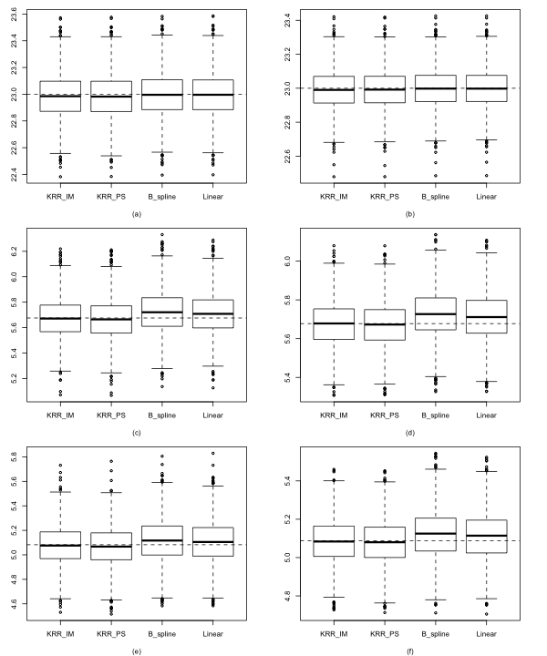
Figure 1: Boxplots with four estimators for model A ((a) for $n=500$ and (b) for $n=1000$), model B ((c) for $n=500$ and (d) for $n=1000$) and model C ((e) for $n=500$ and (f) for $n=1000$) under first response mechanism with true values (dashes). KRR_IM, kernel ridge regression imputation estimator; KRR_PS, kernel ridge regression propensity score estimator.

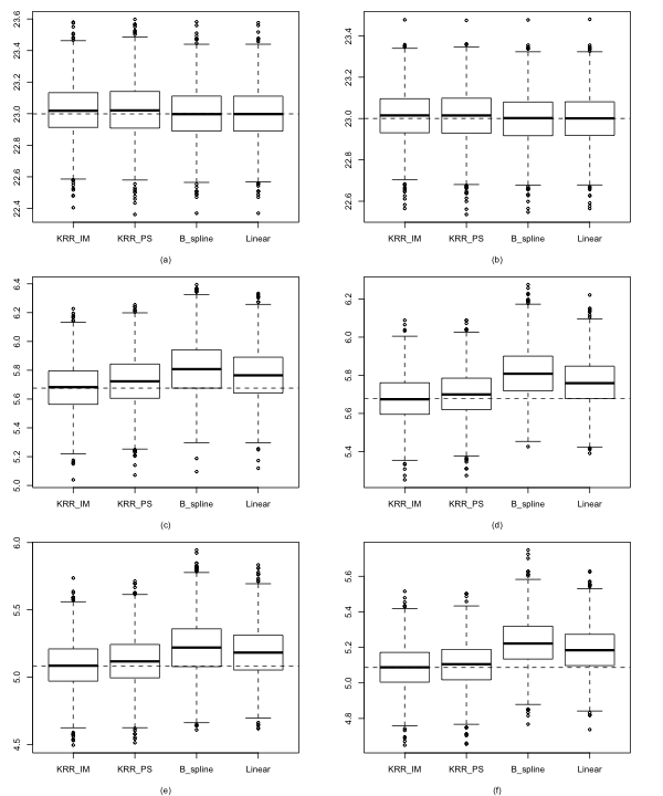
Figure 2: Boxplots with four estimators for model A ((a) for $n=500$ and (b) for $n=1000$), model B ((c) for $n=500$ and (d) for $n=1000$) and model C ((e) for $n=500$ and (f) for $n=1000$) under second response mechanism with true values (dashes). KRR_IM, kernel ridge regression imputation estimator; KRR_PS, kernel ridge regression propensity score estimator.

The simulation results of the four point estimators for the first response mechanism and for the second response mechanism are summarized in Figure 1 and Figure 2, respectively. The simulation results in Figure 1 and Figure 2 show that four methods show similar results under the linear model (model A), but both kernel ridge regression imputation estimators and propensity score estimators show robust performance under the nonlinear models (models B and C). All kernel ridge regression related methods provide negligible biases in all scenarios.

In addition, we have computed the proposed variance estimators under kernel ridge regression imputation with the corresponding kernel. In Table 1, the relative biases (in percentage) of the proposed variance estimator and the coverage rates of two interval estimators under $90\%$ and $95\%$ nominal coverage rates are presented. The relative bias of the variance estimator are relatively low, which confirms the validity of the proposed variance estimator. Furthermore, the interval estimators show good performances in terms of the coverage rates.

Table 1: Relative biases (R.B.) of the proposed variance estimator, coverage rates (C.R.) of the $90\%$ and $95\%$ confidence intervals for imputed estimators and propensity score estimators under kernel ridge regression with second-order Sobolev kernel and Gaussian kernel for continuous responses (KRR_IM, kernel ridge regression imputation estimator; KRR_PS, kernel ridge regression propensity score estimator)

		First Missing Mechanism				Second Missing Mechanism
		KRR_IM		KRR_PS		KRR_IM		KRR_PS
Model	Criteria	n=500	n=1000	n=500	n=1000	n=500	n=1000	n=500	n=1000
	R.B(%)	0.09	-2.80	0.15	-3.14	3.40	2.74	-1.68	-1.90
A	C.R.(90%)	90.30	89.95	90.30	89.75	90.25	90.60	89.15	89.85
	C.R.(95%)	95.50	94.95	95.70	95.00	95.20	95.45	94.65	94.80
	R.B(%)	-2.77	-5.42	-5.77	-6.60	-6.07	-3.42	-11.25	-6.23
B	C.R.(90%)	89.55	89.70	89.20	89.20	88.05	90.05	87.75	89.30
	C.R.(95%)	94.25	94.55	93.85	94.10	94.15	94.70	93.35	94.10
	R.B(%)	-7.43	-3.97	-12.24	-6.22	-9.38	-2.29	-13.62	-4.34
C	C.R.(90%)	87.95	88.70	86.70	88.75	88.80	89.50	87.50	89.75
	C.R.(95%)	93.35	94.20	92.35	93.70	93.95	95.15	93.25	94.70

6 Application

We applied the kernel ridge regression with the kernel of second-order Sobolev space to study the $\mbox{PM}_{2.5}(\mu g/m^{3})$ concentration measured in Beijing, China (Liang et al., 2015). Hourly weather conditions: temperature, air pressure, cumulative wind speed, cumulative hours of snow and cumulative hours of rain are available from 2011 to 2015. Meanwhile, the averaged sensor response is subject to missingness. In December 2012, the missing rate of $\mbox{PM}_{2.5}$ is relatively high with missing rate $17.47\%$. We are interested in estimating the mean $\mbox{PM}_{2.5}$ in December with both imputed and propensity score kernel ridge regression estimates. The point estimates and their 95% confidence intervals are presented in the Table 2. As a benchmark, the confidence interval computed from complete cases and confidence intervals for the imputed estimator under linear model (Kim and Rao, 2009) are also presented there.

Table 2: Point estimates (P.E.), standard error (S.E.) and $95\%$ confidence intervals (C.I.) for imputed mean $\mbox{PM}_{2.5}$ in December, 2012 under kernel ridge regression (KRR_IM, kernel ridge regression imputation estimator; KRR_PS, kernel ridge regression propensity score estimator.)

Estimator	P.E.	S.E.	$95\%$ C.I.
Complete	109.20	3.91	(101.53, 116.87)
Linear	99.61	3.68	(92.39, 106.83)
KRR_IM	101.92	3.50	(95.06, 108.79)
KRR_PS	102.25	3.50	(95.39, 109.12)

As we can see, the performances of kernel ridge regression imputation estimators are similar and created narrower $95\%$ confidence intervals. Furthermore, the imputed $\mbox{PM}_{2.5}$ concentration during the missing period is relatively lower than the fully observed weather conditions on average. Therefore, if we only utilize the complete cases to estimate the mean of $\mbox{PM}_{2.5}$, the severeness of air pollution would be over-estimated.

7 Concluding Remarks

We consider kernel ridge regression as a tool for nonparametric imputation and propensity score weighting. The proposed kernel ridge regression imputation can be used as a general tool for nonparametric imputation. By choosing different kernel functions, different nonparametric imputation methods can be developed. Asymptotic properties of the propensity score estimator are also established. The unified theory developed in this paper enables us to make valid nonparametric statistical inferences about the population means under missing data.

There are several possible extensions of the research. First, the theory can be extended to other nonparametric imputation methods, such as smoothing splines (Claeskens et al., 2009), thin plate spline (Wahba, 1990), Gaussian process regression (Rasmussen and Williams, 2005), or deep kernel learning (Bohn et al., 2019). The theoretical results in this paper can be used as building-blocks for establishing the statistical properties of these sophisticated nonparametric imputation methods. Second, instead of using ridge-type penalty term, one can also consider other penalty functions such as the smoothly clipped absolute deviation penalty (Fan and Li, 2001) or adaptive lasso (Zou, 2006). Such penalty functions can be potentially useful for handling high dimensional covariate problems. Also, the proposed method can be used for causal inference, including estimation of average treatment effect from observational studies (Morgan and Winship, 2014; Yang and Ding, 2020). Developing tools for causal inference using the kernel ridge regression-based propensity score method will be an important extension of this research.

References

- Aronszajn (1950) Aronszajn, N. (1950). Theory of reproducing kernels. Transactions of the American mathematical society 68(3), 337–404.
- Bohn et al. (2019) Bohn, B., C. Rieger, and M. Griebel (2019). A represented theorem for deep kernel learning. Journal of Machine Learning Research 20, 1–32.
- Chan et al. (2016) Chan, K. C. G., S. C. P. Yam, and Z. Zhang (2016). Globally efficient non-parametric inference of average treatment effects by empirical balancing calibration weighting. Journal of the Royal Statistical Society, Series B 78, 673–700.
- Chen and Shao (2001) Chen, J. and J. Shao (2001). Jackknife variance estimation for nearest neighbor imputation. Journal of the American Statistical Association 96, 260–269.
- Chen et al. (2013) Chen, S. X., J. Qin, and C. Y. Tang (2013). Mann-whitney test with adjustments to pretreatment variables for missing values and observational study. Journal of the Royal Statistical Society, Series B 75, 81–102.
- Cheng (1994) Cheng, P. E. (1994). Nonparametric estimation of mean functionals with data missing at random. Journal of the American Statistical Association 89(425), 81–87.
- Claeskens et al. (2009) Claeskens, G., T. Krivobokova, and J. D. Opsomer (2009). Asymptotic properties of penalized spline estimators. Biometrika 96, 529–544.
- Fan and Li (2001) Fan, J. and R. Li (2001). Variable selection via nonconcave penalized likelihood and its Oracle properties. Journal of the American Statistical Association 96, 1348–1360.
- Friedman et al. (2001) Friedman, J., T. Hastie, and R. Tibshirani (2001). The Elements of Statistical Learning, Volume 1. Springer series in statistics New York.
- Hainmueller (2012) Hainmueller, J. (2012). Entropy balancing for causal effects: A multivariate reweighting method to produce balanced samples in observational studies. Political Analysis 20, 25–46.
- Hampel (1974) Hampel, F. R. (1974). The influence curve and its role in robust estimation. Journal of the American Statistical Association 69, 383–393.
- Imai and Ratkovic (2014) Imai, K. and M. Ratkovic (2014). Covariate balancing propensity score. Journal of the Royal Statistical Society: Series B: Statistical Methodology, 243–263.
- Kanamori et al. (2012) Kanamori, T., T. Suzuki, and M. Sugiyama (2012). Statistical analysis of kernel-based least-squares density-ratio estimation. Machine Learning 86(3), 335–367.
- Kim et al. (2014) Kim, H. J., J. P. Reiter, Q. Wang, L. H. Cox, and A. F. Karr (2014). Multiple imputation of missing or faulty values under linear constraints. Journal of Business & Economic Statistics 32(3), 375–386.
- Kim and Rao (2009) Kim, J. K. and J. Rao (2009). A unified approach to linearization variance estimation from survey data after imputation for item nonresponse. Biometrika 96(4), 917–932.
- Kim and Shao (2013) Kim, J. K. and J. Shao (2013). Statistical Methods for Handling Incomplete Data. CRC press.
- Koltchinskii et al. (2006) Koltchinskii, V. et al. (2006). Local Rademacher complexities and oracle inequalities in risk minimization. Annals of Statistics 34(6), 2593–2656.
- Liang et al. (2015) Liang, X., T. Zou, B. Guo, S. Li, H. Zhang, S. Zhang, H. Huang, and S. X. Chen (2015). Assessing Beijing’s PM 2.5 pollution: severity, weather impact, APEC and winter heating. Proceedings of the Royal Society A: Mathematical, Physical and Engineering Sciences 471(2182), 20150257.
- Little and Rubin (2019) Little, R. J. and D. B. Rubin (2019). Statistical analysis with missing data, Volume 793. John Wiley & Sons.
- Mendelson (2002) Mendelson, S. (2002). Geometric parameters of kernel machines. In International Conference on Computational Learning Theory, pp. 29–43. Springer.
- Morgan and Winship (2014) Morgan, S. L. and C. Winship (2014). Counterfactuals and Causal Inference. Cambridge University Press.
- Nguyen et al. (2010) Nguyen, X., M. J. Wainwright, and M. I. Jordan (2010). Estimating divergence functionals and the likelihood ratio by convex risk minimization. IEEE Transactions on Information Theory 56(11), 5847–5861.
- Rasmussen and Williams (2005) Rasmussen, C. E. and C. Williams (2005). Gaussian Processes for Machine Learning. The MIT Press.
- Robins et al. (1994) Robins, J. M., A. Rotnitzky, and L. P. Zhao (1994). Estimation of regression coefficients when some regressors are not always observed. Journal of the American Statistical Association 89, 846–866.
- Rubin (1976) Rubin, D. B. (1976). Inference and missing data. Biometrika 63(3), 581–592.
- Sang et al. (2020) Sang, H., J. K. Kim, and D. Lee (2020). Semiparametric fractional imputation using Gaussian mixture models for multivariate missing data. Journal of the American Statistical Association. Available online (https://doi.org/10.1080/01621459.2020.1796358).
- Scholkopf and Smola (2002) Scholkopf, B. and A. J. Smola (2002). Learning with Kernels. The MIT Press.
- Shawe-Taylor et al. (2004) Shawe-Taylor, J., N. Cristianini, et al. (2004). Kernel methods for pattern analysis. Cambridge university press.
- Steinwart et al. (2009) Steinwart, I., D. R. Hush, C. Scovel, et al. (2009). Optimal rates for regularized least squares regression. In COLT, pp. 79–93.
- Stone (1982) Stone, C. (1982). Optimal global rates of converence for nonparametric regression. The Annals of Statistics 10, 1040–1053.
- Tan (2020) Tan, Z. (2020). Regularized calibrated estimation of propensity scores with model misspecification and high-dimensional data. Biometrika 107(1), 137–158.
- van de Geer (2000) van de Geer, S. A. (2000). Empirical Processes in M-estimation, Volume 6. Cambridge university press.
- Wahba (1990) Wahba, G. (1990). Spline models for observational data, Volume 59. Siam.
- Wang and Chen (2009) Wang, D. and S. X. Chen (2009). Empirical likelihood for estimating equations with missing values. Annals of Statistics 37, 490–517.
- Wang and Kim (2021) Wang, H. and J. Kim (2021). Propensity score estimation using density ratio model under item nonresponse. Unpublished manuscript (Available at https://arxiv.org/abs/2104.13469).
- Wu and Sitter (2001) Wu, C. and R. R. Sitter (2001). A model-calibration approach to using complete auxiliary information from survey data. Journal of the American Statistical Association 96, 185–193.
- Yang and Ding (2020) Yang, P. and P. Ding (2020). Combining multiple observational data sources to estimate causal effects. Journal of the American Statistical Association 115, 1540–1554.
- Yang and Kim (2020) Yang, S. and J. K. Kim (2020). Asymptotic theory and inference of predictive mean matching imputation using a superpopulation model framework. Scandinavian Journal of Statistics 47, 839–861.
- Zhang (2005) Zhang, T. (2005). Learning bounds for kernel regression using effective data dimensionality. Neural Computation 17(9), 2077–2098.
- Zhang et al. (2013) Zhang, Y., J. Duchi, and M. Wainwright (2013). Divide and conquer kernel ridge regression. In Conference on learning theory, pp. 592–617.
- Zhao (2019) Zhao, Q. (2019). Covariate balancing propensity score by tailored loss functions. Annals of Statistics 47, 965–993.
- Zou (2006) Zou, H. (2006). The adaptive Lasso and its oracle properties. Journal of the American Statistical Association 101, 1418–1429.