Combatting Gerrymandering with Social Choice:
the Design of Multi-member Districts

Abstract

Every representative democracy must specify a mechanism under which voters choose their representatives. The most common mechanism in the United States – Winner takes all single-member districts – both enables substantial partisan gerrymandering and constrains ‘fair’ redistricting, preventing proportional representation in legislatures. We study the design of multi-member districts (MMDs), in which each district elects multiple representatives, potentially through a non-Winner takes all voting rule. We carry out large-scale empirical analyses for the U.S. House of Representatives under MMDs with different social choice functions, under algorithmically generated maps optimized for either partisan benefit or proportionality. Doing so requires efficiently incorporating predicted partisan outcomes – under various multi-winner social choice functions – into an algorithm that optimizes over an ensemble of maps. We find that with three-member districts using Single Transferable Vote, fairness-minded independent commissions would be able to achieve proportional outcomes in every state up to rounding, and advantage-seeking partisans would have their power to gerrymander significantly curtailed. Simultaneously, such districts would preserve geographic cohesion, an arguably important aspect of representative democracies. In the process, we advance a rich research agenda at the intersection of social choice and computational gerrymandering.

1 Introduction

This bill requires (1) that ranked choice voting …be used for all elections for Members of the House of Representatives, (2) that states entitled to six or more Representatives establish districts such that three to five Representatives are elected from each district, and (3) that states entitled to fewer than six Representatives elect all Representatives on an at-large basis—Fair Representation Act, H.R. 4000, 2019.

The Fair Representation Act, first introduced in 2017 and reintroduced in 2019 and 2021, would mandate the use of multi-member districts (MMDs) to elect members to the United States House of Representatives, i.e., having fewer, larger districts each with multiple representatives. The bill is supported by good governance organizations such as FairVote [54]; the American Academy of Arts and Sciences in 2020 released a report advocating states to use multi-member districts – however, “on the condition that they adopt a non-Winner takes all election model” [3]. Despite the popular focus on single-member district (SMD) elections, such MMDs have a long history in the United States, especially at the state and local level. In 1962, 41 state legislatures had MMDs, often with Winner takes all models [80]; even today, 10 state legislatures elect representatives for at least one chamber in such a manner – Arizona, for example, has two-member districts, where each voter is given two votes and the top two vote-getters in each district are elected [17, 18], and there is an ongoing debate in Maryland on whether to keep their (Winner takes all) MMDs. City councils, state parties, and other organizations often adopt more sophisticated techniques, using variations on Ranked Choice Voting (RCV) to elect multiple winners from each of several districts [55].

This paper considers the design of such multi-member districts and, in the process, advances a rich research agenda at the intersection of two well-studied aspects of the design of representative democracies: partisan gerrymandering, and social choice for multiple winners. The gerrymandering literature largely assumes Winner takes all in SMDs and, given a fixed set of voters, studies how to divide the voters into districts such that the set of winners across districts satisfies desirable properties (e.g., for a gerrymandering party, maximizing the number of winners belonging to their party; for a neutral rule-maker, devising rules to ensure ‘proportionality,’ such that the fraction of winners of each party matches the fraction of voters). The social choice literature, on the other hand, considers a single district and studies voting rules (functions from voter rankings to a set of winners) such that the set of winners in that district satisfies similar properties, including proportionality. A map consisting of multiple MMDs (e.g., 30 two-member districts in Arizona) requires both partitioning voters into districts and devising how each district collects and aggregates votes. The challenge cannot be decomposed: drawing districts depends on the social choice function, and the same social choice function has different effects depending on district size and composition.

We study this joint challenge, carrying out large-scale empirical analyses for the U.S. House of Representatives under MMDs with different social choice functions, under maps that could be drawn by either partisan gerrymanderers or independent commissions. We show that indeed the choices of (how many and which) districts to draw and which voting method to use should not be made independently. For example, while MMDs with Winner takes all elections are commonly believed to be discriminatory against minorities when compared to SMDs [79, 44, 28], we find that MMDs with more proportional voting methods support political minorities. We further find that ‘interior’ solutions in this joint optimization – with neither SMDs nor one large MMD – often best balance the multiple objectives promoted by good governance groups. In more detail, our contributions and findings are as follows.

Methodological contributions.

We provide a scalable, empirical methodology to algorithmically study partisan gerrymandering and fair redistricting under multi-member districts. We leverage an efficient way to calculate partisan outcomes under Single Transferable Voting (a common variant RCV for multiple winners) and extend an algorithm by Gurnee and Shmoys [61] to efficiently calculate near-optimal multi-member maps, under a variety of objective functions and social choice rules. We further develop an individual-level, voter-file-based methodology to study intra-party effects of ranked choice voting. Our results, using voting and individual-level data from across the United States, further illustrate how theoretical social choice guarantees heterogeneously translate to practice, away from the asymptotic regimes in which they are often studied.

We believe that this work and methodological approach can be applied beyond the context of multi-member districts for legislatures in the United States, for questions regarding the design of representative democracies at the intersection of gerrymandering and social choice, across both the computer and political sciences.

Application-oriented findings.

We apply our methods to consider the design of MMDs, focusing empirically on the House of Representatives in the United States. We primarily study proportionality, as a function of the number of districts and the voting rule used. Surprisingly, our results indicate that two-member or three-member districts with proportional voting rules are often sufficient to prevent the worst gerrymanders by an adversary and to enable independent commissions to find a proportional map – even small MMDs are enough to eliminate “natural” gerrymandering, in which geography and the distribution of citizens leads to a natural advantage for one party, and purposeful ones. This result holds with no other constraints, besides district contiguity.

On the other hand, we find that poor design constraints (in either the number of districts or the voting rule used) enable more extreme gerrymanders than is possible with SMDs. These effects occur because MMDs with appropriate social choice functions protect concentrated (political) minorities by making packing and cracking more difficult, and support diffuse minorities by joining them in the same large multi-member district, with a lower threshold to win a seat. We further analyze H.R. 4000 and show that it achieves an effective balance in the MMD design space—though, as emphasized above, its prescribed three to five member districts are larger than are necessary; this part of the bill could be relaxed without sacrificing its proportionality goals.

Finally, we study how MMDs affect intra-party diversity, measuring two competing claims: that small SMDs protect diverse, geographically-correlated interests within a party (e.g., urban, Black Democrats versus suburban, white Democrats), and conversely that RCV with large MMDs enable ideological differences within a party (cf. [55, 81]). We find, under reasonable assumptions on how voters rank candidates within a party, that two- or three-member districts preserve geographic compactness, and thus the notion that legislature members represent a geographically cohesive set of voters.

Section 2 contains our model and methods. Section 3 contains our main results, regarding inter-party effects of multi-member districts. Section 4 considers intra-party effects. We conclude in Section 5 with a theoretical, empirical, and practical agenda for the intersection of gerrymandering and social choice.

Related work

This work is at the intersection of two rich literatures, showing how joint optimization over how voters are split into districts (gerrymandering) and how they vote within a district (social choice) yields outcomes that neither could achieve separately. It further contributes to the literature studying multi-winner districts in the United States. Given each field’s vast literature, we focus on the most relevant work.

Redistricting

Gerrymandering is the practice of using district boundaries to engineer electoral outcomes by “packing” and “cracking” voters within and between districts [65, 52, 75]. Past computational research has almost exclusively studied gerrymandering and redistricting more broadly in the context of a fixed number of single-member districts with Winner takes all elections.

Optimal political districting is well known to be an NP-hard computational problem [84, 69, 33]. Therefore, to study redistricting, researchers have developed ensemble methods [43, 72, 34, 11, 57, 73, 61, 12] that generate huge quantities of legal district plans to explore the exponentially large space of feasible maps. Such techniques are commonly used to detect gerrymandering [36, 46, 48, 64, 63] or to study the impact of different redistricting rules on the distribution of outcomes [41, 42]. An important result is that even under ‘neutral’ maps drawn without regard to underlying political geography, the natural geographic segregation among partisan voters can create skewed political outcomes [24, 34].

There are many proposed metrics of fairness in redistricting, including: the efficiency gap [90], the mean-median gap [101], partisan-symmetry [102], competitiveness [42], and most simply, proportionality. Such metrics can be used as the objective function of an optimization algorithm to generate district maps with (un)fair outcomes [92, 61, 67, 29]. However, because of partisan segregation, in some states creating a proportional plan with SMDs is actually impossible [47], motivating the use of alternate election procedures. In this work, we primarily consider proportionality as our fairness notion.

Inspired by the fair division literature, researchers have also recently proposed methods in which two adversarial parties together draw a map [23, 22, 82, 96].

Social choice

The social choice community, on the other hand, considers a fixed set of voters and number of winners in a given election. Then, it considers various voting rules (how preferences are elicited and aggregated) affect the outcome [25, 10, 45]. Here, we focus on the literature on multi-winner elections. The theoretical social choice literature considers properties of voting rules, often for arbitrary distributions of voters [30, 70, 13, 51, 37, 14, 58, 35]. Most relevant is Skowron [88], which studies the proportionality guarantees of various multi-winner voting rules, including Thiele rules; they find Proportional Approval Voting (a type of Thiele rule) to be the most proportional, though other Thiele methods may outperform it on other metrics. The optimality of PAV and the parametrizable nature of the class motivates us to focus on Thiele rules in this work, and our results complement the theoretical work in comparing such rules in non-asymptotic settings with empirical voter distributions. Related to our intra-party analysis, Elkind et al. [50] simulate the properties of multiwinner voting rules (such as STV and PAV) when voters lie on a two-dimensional Euclidean space.

On the applied side, a strand of the literature studies the effects of voting reforms, especially on minority voters. McDaniel [74] find that RCV increased racially polarized voting in comparison to run-off elections. McGhee and Shor [76] find mixed evidence for whether top-two primaries have reduced polarization, and Rogowski and Langella [85] find no evidence that open vs closed primaries affect candidate ideology; Grose [60] finds the opposite on both points. Spencer et al. [89] advocate for ranked choice voting as a Voting Rights Act remedy, supporting its legality.

Multi-member districts in the United States.

As chronicled by Klain [68] in 1955, there is a rich history of multi-member districts in the United States in state legislatures and city councils. In 1962, for example, 30 states used MMDs to elect state senators, and 41 states used them to elect state representatives, mostly in two- to four-member districts with Winner takes all procedures [80]. Historically, at-large city council members have often also been elected with equivalent procedures. On the other hand, since 1967 federal law has banned the use of MMDs to elect members to the U.S. House of Representatives, a status quo H.R. 4000 would repeal.

The political science community has studied these districts, often focusing on their effect on race [87, 39, 19], though some have questioned the optimal district size [62]. In particular, while the empirical evidence is mixed due to the observational nature of analysis, the predominant view is that Winner takes all MMDs harmed racial minorities, especially in Southern states [79, 44, 28]. Similarly, Winner takes all at-large city council elections are thought to dilute the votes of minorities [91, 27, 100, 95, 40]. As theoretical models [59] elucidate, such districts with Winner takes all rules enable the majority – even without substantially distorting district lines as might be necessary with SMDs – to ensure that a minority even with 49% of the vote elects none of its preferred candidates. Partially due to such evidence, by 1982 the majority of states had eliminated the use of MMDs for their state legislatures, and several cities have eliminated their at-large council seats under court mandate. Most recently, Lempert [71] analyzes the legality of RCV and multi-member districts, and advocates for it as a court-ordered remedy to illegal gerrymanders.

Most related is work favorably comparing MMDs using ranked choice voting to SMDs for city councils. Benade et al. [21] compare outcomes using RCV versus single-member districts in four empirical case studies, finding that it yields better representations for demographic minorities. From the same group, Buck et al. [26] and Angulu et al. [4] propose using RCV with several MMDs instead of SMDs for the Lowell, MA and Chicago, IL city councils, respectively. Their work primarily considers non-partisan representation, such as race and other demographic characteristics – these factors are more salient in municipal contexts, where such MMDs with RCV are more common today. Our Section 4 explores similar questions, with complementary voter-file based methods. More recently in subsequent work, the MGGG Redistricting Lab [78] also analyzes the effects of the Fair Representation Act, though with a more limited set of district sizes and focusing on racial representation.

To this literature, our work adds a systematic analysis of the partisan effects of such districts: providing a scalable methodology, characterizing the effects on proportional representation under both adversarial gerrymandering and ‘fair’ redistricting across the range of possible district sizes, and providing design recommendations for legislation. We further study how MMDs affect intra-party results on two dimensions, political preference and geography.

Other political solutions.

Finally, we note that multi-member districts are far from the only possible governmental system to achieve proportionality or other related desiderata. Many countries have seat allocation systems designed to be proportional with multiple parties (see Pukelsheim [83] for a survey), and there are other proposals to achieve such goals in the United States (e.g., [16]). Such systems have also been studied in the EconCS and Operations communities (e.g., [53, 32, 31]). For example, Bachrach et al. [15] consider the misrepresentation ratio of single-member districting with various score-based ranking rules, in Electoral College type settings: when these rules are used to elect a winner within each district but then an overall winner is declared based on the majority vote of districts. A comparative analysis of such approaches—and especially which may be most politically feasible in various jurisdictions—is out of the scope of this work.

2 Model and methods

Section 2.1 formalizes the joint redistricting and social choice challenge, Section 2.2 introduces the social choice functions we analyze and shows how to efficiently compute per-party seat shares under them, and Section 2.3 presents our empirical method.

2.1 Problem definition

The task is to elect a legislature composed of $N$ seats. There is a population of voters $\mathcal{V}$; each voter $v\in\mathcal{V}$ lives in an atomic block $b_{v}\in\mathcal{B}$ and belongs to a party $p_{v}\in\{R,D\}$. The blocks $\mathcal{B}$ are organized in an adjacency graph where two blocks share an edge when they are geographically adjacent to each other.

Multi-member redistricting.

In redistricting, the blocks $\mathcal{B}$ are partitioned into $K$ geographically contiguous districts, where each district $k$ is allocated $N_{k}\in\mathbb{N}$ seats in the legislature such that $\sum_{k}N_{k}=N$, and $N_{k}\geq 1$. Each district also must be population balanced in accordance with $N_{k}$, such that the population ratio of district $k$ to the whole state is bounded between $\frac{N_{k}\pm\epsilon}{N}$ for population tolerance $\epsilon$. The resulting set of districts is referred to as a map or a plan. Maps can be drawn to fulfill various objective functions. For example, a party can gerrymander a map to maximize the seats won by their party, or an independent commission can attempt to satisfy one or more notions of fairness.

Social choice function.

Each district runs a separate election to fill its $N_{k}$ seats, with each voter $v$ voting in the district $k(b_{v})$ to which its block $b_{v}$ belongs. Each election is run according to a social choice function $F$ that determines what information each voter provides (in this work, either a set of approved candidates or a ranking over candidates) and how votes are aggregated, to produce the $N_{k}$ winners in each district $k$.

Together, the choice of map ($K$ contiguous districts with $N_{k}$ seats each) and social choice function $F$ define an election. Given data on voters and assumptions on how they rank candidates (detailed in Section 2.2), the procedure determines the set of $N$ winners. (In our empirical approach throughout, we use a probabilistic approach to compute the expected seat-share based on the variance of past elections to model the heterogeneous political elasticity and noise among different constituencies.)

Evaluation metrics.

An election procedure can be evaluated based on the set of winners it produces. To measure outcomes across parties, we primarily consider proportionality: how does the fraction of winners $w_{p}$ belonging to each party $p\in\{R,D\}$ (seat share) compare to the fraction of voters $y_{p}$ (vote share); the proportionality gap is the difference $|w_{R}-y_{R}|$. The larger the gap, the more that the procedure favors one party over another. In Section 4, we further consider intra-party measures, i.e., how the election procedure influences within-party differences.

Research questions.

We ask: how does the election procedure determine the induced outcomes, and what is the joint influence of the social choice function $F$ and the map? Note that the various components of the election procedure may be determined by different actors with competing interests. H.R. 4000, for example, would mandate that $N_{k}\in\{3,4,5\}$ and a RCV-based social choice function be used. However, barring a separate mandate concerning independent commissions, in each state a partisan state legislature may still seek to draw maps most favorable to their party. Thus, we in particular are interested in the following design question: how do various constraints on the election procedure design space (restrictions on $K$, $N_{k}$, or $F$) affect the range of outcomes possible, under maps drawn by either partisan actors or independent commissions?

2.2 Social choice functions, voter assumptions, and calculating seat shares

We study our research questions empirically, analyzing outcomes under counterfactual election procedure designs. However, doing so requires converting historical voting data to expected electoral outcomes under various social choice functions and with hypothetical candidates. Further, outcomes must be able to be efficiently computed, as our redistricting optimization algorithm (introduced in Section 2.3) calculates as a sub-routine the seat share under a given district and social choice function. We now lay the groundwork for our empirical method, by introducing our social choice functions and assumptions and showing how to efficiently compute per-party seat shares in a district.

Social choice functions considered.

We consider two well-studied classes of social choice functions from the literature: Thiele rules and Single Transferable Vote (STV).

A Thiele rule is characterized by a function $\lambda$. Each voter $v$ in district $k$ provides a set $S_{v}$ of the $N_{k}$ candidates they like most. The set of winners are determined as follows. Consider a potential set of winners $C$. The amount of points that voter $v$ contributes to $C$ is $\sum_{i=1}^{|S_{v}\cap C|}\lambda(i)$, and the set $C$ with the most points across voters (after tie-breaking) is selected. The (non-increasing) function $\lambda$ establishes that votes have diminishing returns; the $i$th approved-of candidate in the set is worth $\lambda(i)$. For example, Winner takes all approval voting is a Thiele rule with $\lambda(i)=1$: for each voter, the set $C$ receives a number of points equal to the number of candidates in the set that the voter likes, and so the $N_{k}$ candidates with the most votes win. We further consider Proportional Approval Voting (PAV), a Thiele rule with $\lambda_{\text{PAV}}(i)=\frac{1}{i}$; and Thiele Squared, with $\lambda_{\text{TS}}=\frac{1}{i^{2}}$. PAV is well-studied in the theoretical social choice literature and comes with optimality guarantees (in terms of proportionality) [88]. We use Thiele Squared as a benchmark for the extent to which a social choice function can induce a balanced (but not necessary proportional) legislature.

In Single Transferable Vote (STV), a type of ranked choice voting for multiple winners, each voter instead submits a ranking over candidates. Consider a district with $N_{k}$ seats and $V_{k}$ voters; the set of winners is created iteratively, as follows. The number of first place votes for each candidate is counted. Any candidate with a number of votes at least the “Droop” threshold $Q=\lfloor\frac{V_{k}}{N_{k}+1}\rfloor+1$ is selected as a winner, and their surplus votes (number of votes minus $Q-1$) are transferred to each voters’ next preferences. If no candidate has enough votes, then the candidate with the least number of votes (with tie-breaking) is eliminated, and their votes are transferred. The process continues until $N_{k}$ candidates have been selected, or the number of remaining candidates equals the number of remaining seats. STV is commonly used in practice in multi-winner elections.

Details can differ on how such votes are transferred, but our results in Section 3 do not depend on how they are; in our simulations in Section 4, we use the Scottish (or “fractional”) STV rule, in which each voter keeps a fractional number of votes equal to their share of the winning candidate’s surplus votes. For consistency, for all rules we assume that ties are broken in favor of candidates from party $D$, but randomly within each party.

Voter assumptions.

Next, we require assumptions on how voters rank or approve candidates. For each Thiele rule, we assume that in each district $k$ there are exactly $N_{k}$ candidates from each party, and each voter simply approves all the candidates in their party. For STV, we assume that in each district $k$ there are at least $N_{k}$ candidates from each party, and that parties are solid coalitions [49]: that each voter ranks all candidates of their party over each candidate of the other party, though intra-party rankings may vary. These assumptions reflect that party membership is a strong predictor of the party of the candidate for which a voter votes. Such an assumption, using historical party vote shares to predict vote shares in future elections, is used throughout the redistricting literature for SMDs; our additional assumption is that this behavior extends to partisan voting in multi-member elections. Section 4, on intra-party effects, studies a setting without such a solid coalitions assumption.

Calculating seat share given vote shares.

Suppose – for a given district with $N_{k}$ seats and $V$ voters – we know the fraction $y_{p}$ of voters that belong to each party $p\in\{R,D\}$ (vote share). How do we calculate the number of winners $n_{p}$ from each party for a given social choice function?

Given our assumptions, it is straightforward to efficiently do so for Thiele rules, as candidates from a given party receive the same votes—and so we do not have to consider individual candidates, only the number of winners from each party directly. Then, we have that the party R seat share is:

$$n_{R}(y_{R},\lambda)=\min_{n}\left[\operatorname*{arg\,max}_{n}\left[y_{R}\sum_{i=1}^{n}\lambda(i)+(1-y_{R})\sum_{i=1}^{N_{k}-n}\lambda(i)\right]\right].$$ (1)

The outer $\min$ encodes tie-breaking in favor of party $D$, and the inner $\operatorname*{arg\,max}$ comes directly from the rule definition. The party D seat share is $n_{D}(y_{R},\lambda)\triangleq N_{k}-n_{R}(y_{R},\lambda)$.

On the other hand, in STV, candidates of the same party may have different numbers of votes (in any round), as intra-party voter rankings may be arbitrary. One may thus, naively, believe that calculating party seat shares would require further assumptions on voter behavior (on voters’ intra-party rankings) and carrying out the iterative procedure defined above, as the elimination and transfer scheme introduces substantial path dependence across candidates and rounds; in general with arbitrary voter rankings, such calculations are required. Doing so, with many voters and candidates, would be prohibitively computationally expensive as a subroutine in a redistricting optimization algorithm. The following proposition establishes that under our assumptions, party seat shares can be efficiently calculated just from the vote shares, without dependence on voter rankings.

Proposition 1 (Seat shares under STV).

Suppose – for a given district with $M$ seats and $V$ voters – that a fraction $y_{p}$ of voters belong to each party $p\in\{R,D\}$, and that there are at least $M$ candidates per party. Assume that each party’s voters rank all same-party candidates above all other-party candidates, and ties are broken in party D’s favor.

Let $n_{R}(y_{R},STV)$ be the number of winners belonging to party $R$ using STV. Then, $n_{R}(y_{R},STV)$ is the unique integer such that

$$y_{R}\cdot(M+1)-1\leq n_{R}(y_{R},STV)<y_{R}\cdot(M+1).$$ (2)

Further, STV is equivalent to proportional approval voting (PAV) for partisan seat share,

$$n_{R}(y_{R},\text{STV})=n_{R}(y_{R},\lambda_{\text{PAV}}).$$ (3)

At a high level, the proof establishes that no candidate receives meaningful (in terms of party vote share) votes from voters of the other party; in terms of party vote share, we can proceed with running two separate STV processes. Then, the sequential round path dependence does not matter, as the overall number of first place votes for candidates of each party is invariant, and so the final partisan outcome depends just on initial vote shares. We note that the proof does not depend on our assumption of fractional STV; other transfer rules (such as random voter transfer) that preserve the number of surplus votes would induce identical seat shares.

Importantly for this work, 1 enables calculating party seat shares in a district that uses STV, without needing to (either computationally or data-wise) consider voters’ individual rankings – substantially simplifying the task for a (human or algorithmic) map drawer. As explained next in Section 2.3, we leverage this result to draw gerrymandered and fair maps for STV. Note that the equivalence between PAV and STV is not true in general [56]. We use the equivalence for the setting in this work to transfer intuition from PAV to STV.

Discussion of solid coalitions assumption

A core rationale for ranked choice voting is that it allows elicitation of preferences beyond two-party identity; our primary methods, assuming solid coalitions, does not capture this rationale. However, we believe that the assumption is suitable for the goals of this paper, to study partisan implications of MMDs in the United States. The US has single winner elections for the executive (president, governor) and so will tend toward two parties for those offices. While it is possible that solid coalitions substantially breaks for legislatures with MMDs, it is at least equally reasonable that the 2 party structure approximately remains, with sub-parties nested within them (preserving 2 party solid coalitions): split ticket outcomes between the President/House is increasingly non-existent. That being said, formally extending results beyond solid coalitions is of substantial interest. The technical hurdle is finding an alternative assumption that (1) is believable for the political context, and (2) does not require simulating STV within the inner loop of a redistricting optimization, which is computationally prohibitive at scale. In other words, studying gerrymandering with social choice as we do requires some assumption to enable efficient calculation of seat shares in each district, without simulation of elections. For example, more recent work by MGGG Redistricting Lab [78] uses the same assumption as we do when generating maps, but then simulates ranked choice votes beyond solid coalitions (as we do in Section 4) given those maps; their results, focusing on racial representation, are similar to ours.

We believe that finding a more reasonable assumption than (approximate) solid coalitions – that is still suitable for optimization – for the entire United States is unlikely, but such assumptions could be reasonable for specific political contexts (i.e., awareness of possible third parties or coalition splits that would form within a state). We leave such analysis, and especially an empirical validation of robustness to solid coalitions, for future work after more RCV elections have been run in the United States. Section 4 does analyze the role of intra-party preferences.

2.3 Empirical method

We study our research questions empirically, in the context of the United States House of Representatives. At a high level, we proceed as follows, separately for each state. Given historical voting data, we algorithmically generate maps for each state, social choice function $F$, and district size $K$: the most gerrymandered map for each party (the map that, given the voter data and the social choice rule, would produce the most winners from that party), the map with the smallest proportionality gap, and a neutral ensemble of random maps. For each map, we then calculate our metrics of interest for the relevant social choice rule. We detail steps of this process next. In Section 4, we simulate full STV elections to study intra-party effects and detail the relevant methodological differences there.

Data.

To calculate partisan seat shares, we require vote shares in each atomic block that will be used to compose districts. For each multi-district state, we use the geography matched precinct-level statewide election returns from multiple election data repositories [77, 38, 98, 99, 5, 9, 8, 7, 6] for elections since 2008, aggregated by Gurnee and Shmoys [61]. We filter these results to just Republican and Democratic candidates and average the two-party vote share across elections at both the block-level and the state-level. For the atomic geographic blocks, we use census tracts, with population counts provided by the 5-year American Community Survey estimates. As a general caveat, given the infrequency of statewide elections, these averages are noisy and sensitive to the idiosyncrasies of each race, candidate, and political environment, as well as true underlying shifts over time.

For the intra-party analysis in Section 4, we further require individual-level characteristics that can be used to simulate voter rankings. There, we use a voter file provided to us by a private election analytics company, with individual level voter data: in each block, an anonymized list of voters, along with their (potentially modeled) demographics (including ethnicity, gender, census block of home address); each voter is further assigned a party (either modeled or ground truth in states with party registration) and is scored on several ideological dimensions through a mixture of methods, including survey modeling, ecological inference, and individual level voting history. We calibrate the voter file to match the calculated party vote shares, by sub-sampling the voters according to their assigned party.

Generating maps.

To generate maps, we extend the stochastic hierarchical partitioning (SHP) algorithm by Gurnee and Shmoys [61], which recursively samples subdivisions of a state to create a large random ensemble of population constrained and contiguous districts. These subdivisions are organized into a tree of nested regions that implicitly encodes an exponential number of distinct maps. We extend the original tree growth logic to guarantee the existence of a split with child nodes each able to produce appropriately sized districts for a given MMD size policy. Each district (leaf node) is scored by expected party seat share for each social choice function, and the tree can be efficiently traversed with a dynamic program to select the most gerrymandered map, or the tree leaves can be gathered into a secondary integer program to select the districts which create the most fair plan (for arbitrary definitions of fairness). To ensure robustness, we estimate the variance of vote-share to calculate the expected seat-share per district and optimize for this expectation, rather than simply optimizing for the number of strict majority seats. This prevents, for example, the algorithm from drawing districts in which the historical vote share was 50.1% for one party and declaring them safe seats for that party. We note that this also empirically lessens the sensitivity to the solid coalitions assumption, if historical variance correlates with crossover votes in STV.

All details of the original Stochastic Hierarchical Partitioning (SHP) algorithm can be found in the paper by Gurnee and Shmoys [61] and associated appendices; we further use their same geographic and electoral data (see Appendix Table 2 of Gurnee and Shmoys [61]). Here, we discuss the relevant algorithmic parameters and necessary modifications. We plan to make our github public. The main algorithmic difference from the original SHP algorithm is that we adapted ours to generate multi-member districts. To do this, instead of parameterizing a sample tree node by a region $R$ and total number of seats $s$, we needed to also specify the number of districts that node contains. This is required because at an intermediate node, the number of districts is not immediately derivable from the total number of seats in that node because of ambiguity in the number of $N_{k}$ versus $N_{k}+1$ sized districts. Therefore, the number of seats is used just to balance population, and the number of districts is used for all other tree operations (sampling valid splits, maintaining balance, etc.).

For each pair (state, $K$), with $K\in\{2,3,\dots,10,12,\dots,20,23,\dots 53\}\cup\{N\}$ and $K\leq N$, we sampled the root node $\left(\frac{1000}{K}\right)^{1.2}$ times and each internal node $\left(\frac{300}{K}\right)^{0.5}$ times. These constants were chosen to balance computational cost and optimization quality. We used random-iterative center selection with Voronoi-weighted capacity matching to sample region centers and sizes. All districts are population balanced within a $1\%$ tolerance. Each of these ensembles were then scored, optimized, and subsampled to create a final distribution over partisan outcomes. For the subsample used to calculate the distribution of outcomes under “neutral” maps, we use $1500\sqrt{K}$ maps for each (state, $K$) pair. The number over which the “optimal” maps (most fair, most gerrymandered) are calculated is more complicated: these maps are implicit in the tree structure. For each setting, there are between $10^{3}$ (smallest states) and $10^{12}$ (largest states, most districts) such implicit maps.

Comparison to other methods

We adopt this approach rather than the standard recombination Markov chain algorithm [43] and related local update methods [57, 11, 73, 29, 12] to more efficiently model both partisan and nonpartisan mapmakers under multiple social choice functions. Our approach generates just one district ensemble (set of districts as leaf nodes of the tree), that can then be combined into one of exponentially many valid maps (in number of districts), optimizing each objective under each modeling scenario; in contrast, a single neutral recombination map ensemble would be unlikely to capture the full range of potential partisan gerrymandering under every setting, necessitating the use of a separate biased chain optimized for each combination of party and voting rule and increasing the amount of computation by almost an order of magnitude. Furthermore, in a policy setting with a variable number of districts (as in H.R. 4000), a single hierarchical sample tree produced by SHP can efficiently capture all possible combinations of district sizes. In contrast, recombination would likely require running 29 separate chains for the 29 different combinations of three-, four-, and five-member districts to fill California’s 53 seats under H.R. 4000 rules (times each combination of party and social choice rule for the full experiment). For example, MGGG Redistricting Lab [78] when studying the effects of the Fair Representation Act consider just one combination of district sizes per state.

On the other hand, an advantage of recombination methods is that they sometimes come with guarantees of the sampling distribution over maps, while no such analysis is available for the SHP algorithm. However, in the context of SMDs, [61] find that the SHP finds maps more extreme than do other methods.

Our experiments.

Putting things together, for each generated map, we can simply calculate our metrics of interest. We carry out the process for each social choice function and each state with 2 or more seats in the House, fixing as $N$ the number of seats allocated to that state after the 2010 census. The number of districts $K$ is varied from $1$ (a large MMD with $N$ seats) to $N$ (only SMDs). For each $K$, the set of district sizes $\{N_{k}\}$ is selected such that all districts differ in size by at most one seat, except in the analysis of H.R. 4000.

Overall, generating districts and calculating the metrics utilized over 40 CPU-weeks of computation, not counting the full STV elections simulated in Section 4.

3 Results: Inter-party balance with multi-member districts

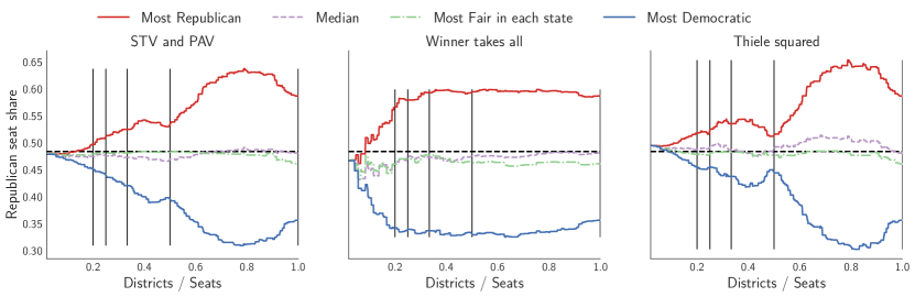
Figure 1: The Republican seat share over all states as the number of districts is varied in each state. The horizontal line denotes the vote share fraction, i.e., the proportionality value. Each point is composed of every state, with rounding, and vertical lines correspond to when $N/K$, the average number of seats per district, is an integer (up to rounding). For example, the vertical line at $0.5$ corresponds to two-member districts in states with an even number of seats, and all two-member districts except one one-member or three-member district in states with an odd number of seats. The right-most point is with SMDs, and the left-most point is if each state has one large MMD. “Median” refers to the median value found across random maps from the SHP algorithm, and “Most fair in each state” to the maps with the smallest proportionality gap. Overall, MMDs are effective at preventing the worst gerrymanders, especially with non-Winner takes all rules. Note that national seat share with Median and Fair maps only look invariant to district size because gaps cancel out between states (some favor Democrats, others Republicans). Figure 2 shows that seat share is not invariant at the per-state level: even when optimizing for fairness, we require MMDs to reduce the per-state proportionality gap.

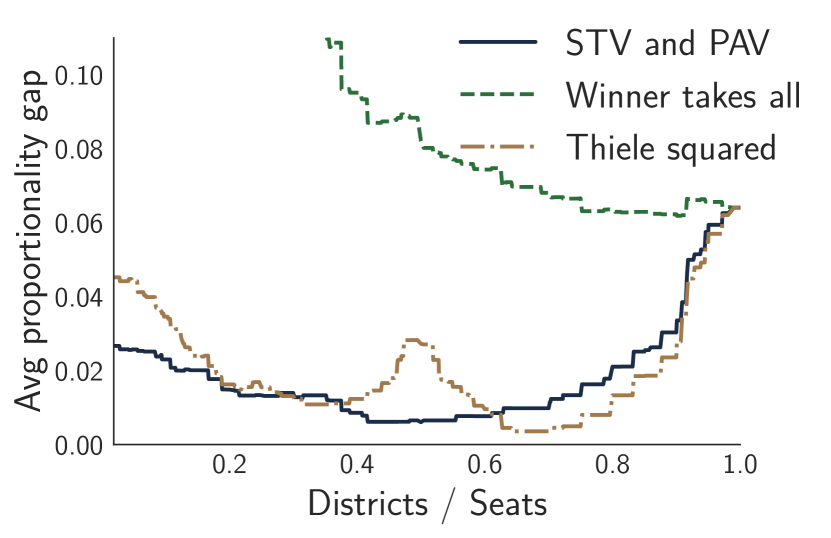
(a) Avg per-state magnitude of gap in “Most Fair” maps

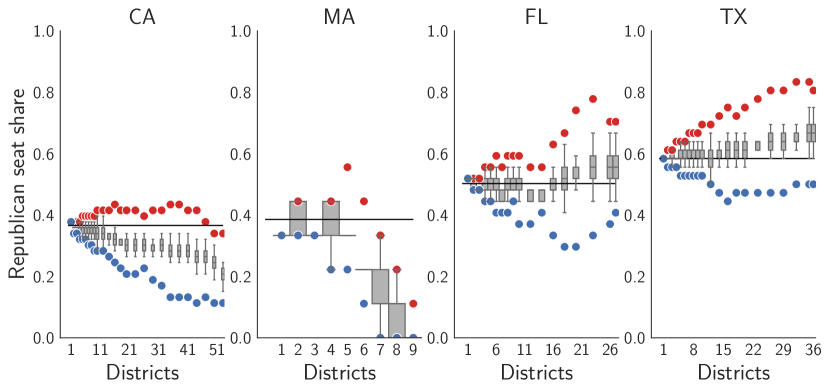
(b) Partisan lean distribution under STV and PAV

Figure 2: How the partisan lean and proportionality gap vary at the state level with voting method and the number of districts. (a). The absolute value of the state-wise proportionality gap in the “Most Fair” map in each state. Even if a redistricting agent wanted to close the proportionality gap, it could not do so with SMDs. (b). The per-state version of Figure 1, showing the full distribution of maps and the extreme gerrymanders. While there are substantive state-level gaps with SMDs even in the most proportional maps, the gaps become negligible with even just two-member districts and STV. Note that in Figure 1, these gaps cancel out nationally, as some state-wise gaps favor Democrats and others favor Republicans. Qualitatively similar results to (a) are shown for the Median and gerrymandered maps in Appendix Figure 7, and plots for all states as in (b) are in Appendix Figure 5.

We begin our analysis by analyzing how MMDs affect partisan balance, both in how MMDs empower independent commissions and in how they constrain adversarial partisan gerrymanderers. Section 3.1 contains our main results; we illustrate the effects of each social choice function and district size, for both extreme gerrymanders and fair redistricting. In Section 3.2, we turn to design questions, discussing the effect of the Thiele rule parameter and heterogeneity across states in terms of ‘optimal’ district size; here, we further analyze how H.R. 4000 navigates such tradeoffs.

3.1 Mitigating gerrymandering with multi-member districts

Figure 1 contains our main result; for each social choice function, it shows how the overall (across states) partisan seat share varies with the number of districts. Figure 2 zooms in on the state level.

Preventing intentional gerrymanders.

MMDs are effective at preventing the most extreme gerrymanders, but only with non-Winner takes all rules. As expected, in the limit, with one large MMD in each state and using STV (equivalently, PAV), the proportionality gap in each state is negligible. Perhaps more surprisingly, just moving from SMDs to two-member districts provides about half the benefit in terms of reducing the proportionality gap for the most extreme gerrymanders.

What explains these results? With SMDs, an R gerrymander would draw a map such that as many districts as possible have a majority of Rs (up to a tolerance for robustness). It does so by cracking, creating many districts in which the D vote share is just below $\frac{1}{2}$ (thus electing an $R$ candidate), and, as necessary, packing, creating a few districts in which the D vote share is as close to 1 as possible. Such a map would maximize D wasted votes. Now, consider PAV, i.e., a Thiele rule with $\lambda(i)=\frac{1}{i}$, and two-member districts. Any district in which the D vote share is between $\frac{1}{3}$ and $\frac{2}{3}$ would elect one member from each party. Cracking thus requires creating districts in which the D vote share is less than $\frac{1}{3}$. Packing means targeting the D vote share to be just below $\frac{2}{3}$ (e.g., a D vote share of $0.6$ to elect one member for each party), or close to $1$ but then giving up both seats in the district. In each case, gerrymandering requires more precision and wastes fewer votes for the opposing party. Simultaneously, fewer districts to draw reduces the degrees of freedom available. The corresponding bands become narrower as district size increases, and similar arguments apply to other Thiele rules with strictly decreasing $\lambda$.

The trend toward proportionality is not monotonic; a mixture of district sizes increases degrees of freedom, enabling gerrymanders even more extreme than do SMDs. Consider two- and one- member districts; the gerrymandering party R could then pack or crack party D in the one-member districts, and use the two-member districts to elect one candidate from each party with R vote share just above $\frac{1}{3}$. Similarly, an urban gerrymandering party D could waste fewer votes winning one-member urban districts, while still getting above $\frac{1}{3}$ of the vote in two-member rural districts. The pattern repeats, to a lesser extent, between every integer division.

Enabling proportional redistricting.

The above analysis considers the most extreme gerrymanders. However, commissions that draw ‘fair’ maps are increasingly common; we now show that MMDs enable the drawing of proportional maps that would not be possible under SMDs. Consider Figure 2(a), which shows the average absolute proportionality gap in each state for the map that minimizes this gap. We find that there is a substantive state-level gap that virtually disappears – up to rounding with a fixed number of districts – even with two-member districts and STV.

Figure 2(b) further demonstrates the SMD ‘Massachusetts problem,’ as elucidated by Duchin et al. [47], and shows that MMDs fix it; because of how evenly Republicans are distributed (diffused) across the state, there is no way to draw SMDs such that a proportional amount of Representatives are Republican. Intuitively, suppose party R has vote share $\frac{1}{3}$. With SMDs, to achieve proportionality a commission would need to draw districts such that party R is in the majority in $\frac{1}{3}$ of the districts, which may not be possible or may require atypical, contorted maps.

A single MMD with PAV provably, approximately achieves proportionality [88], solving the Massachusetts problem up to rounding. Our results indicate that even multiple two-member districts enable fair maps and solve the problem in practice. Intuitively, in the above example, a commission would just need to draw a map with enough districts with R vote share above $\frac{1}{3}$. Note that, by the pigeon-hole principle, with overall party $p$ vote share $v_{p}$, for any map there will always be at least one district in which its vote share is at least $v_{p}$; so, as the threshold to win 1 seat decreases with district size, an ever-smaller minority party is guaranteed at least one seat.

Finally, we note that, as illustrated by the average proportionality gaps of the “Median” maps in Appendix Figure 7, even small multi-member districts with PAV or STV eliminate the issue of ‘natural’ gerrymanders, in which even ‘neutral’ maps – drawn by a redistricting algorithm that ignores partisan vote shares – favor one party, due to the natural geographic distribution of voters. Such natural gerrymanders have played a central role in discussion of a justiciable gerrymandering standard; our results indicate that with even small MMDs, an independent commission would not need to draw maps that substantially differ from neutral maps in order to achieve proportionality.

Competitiveness.

Up to now, we have primarily considered proportionality – how the partisan seat share reflects the underlying vote share in each state. Here, we consider competitiveness – the average margin of victory for the marginal seat in each district. For example, in a Winner takes all election, a Republican vote share of 0.6 in a district would lead to a margin of victory of 0.1. In a PAV election with two winners, the same district would have a victory margin of $(\frac{2}{3}-.6)$, as a Republican vote of $\frac{2}{3}$ (with appropriate tie-breaking) would lead to two elected Republicans as opposed to one. While competitiveness is a controversial as a goal for redistricting (as an objective when drawing maps) [42], it is considered an important dimension along which to evaluate a map. Uncompetitive districts, for example, could depress participation or contribute to polarization.

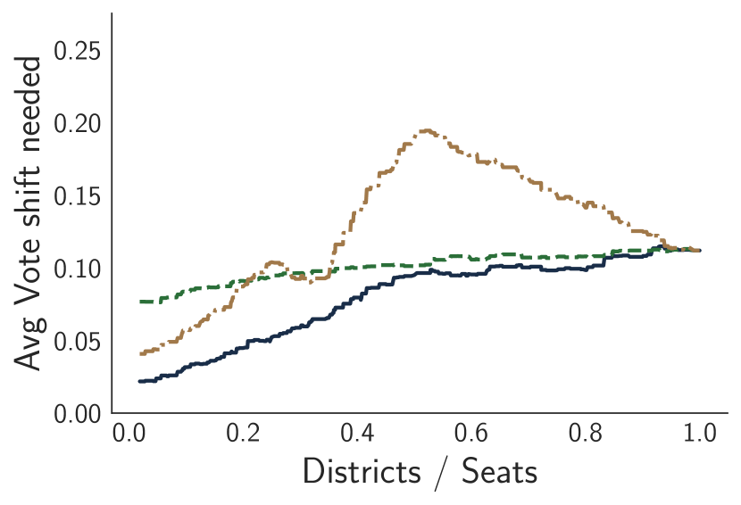
(a) Median map

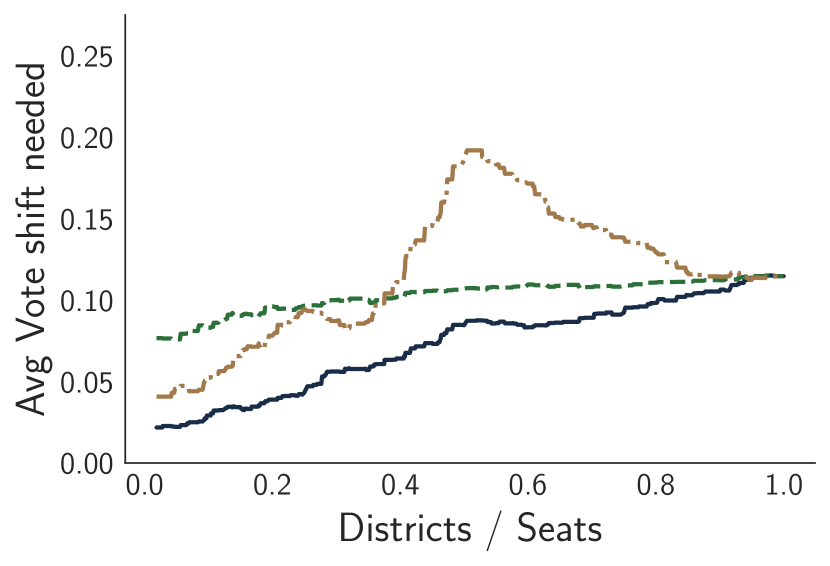
(b) Most fair map

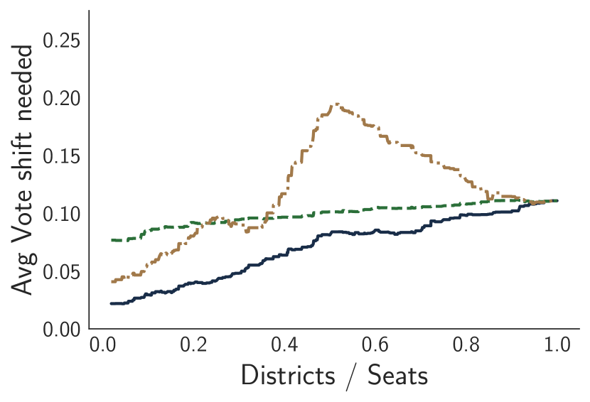
(c) Most Republican

(d) Most Democratic

Figure 13: The average vote shift needed in each map (averaged across districts in a map and across states) to shift the number of seats won by each party by at least one. The larger the vote shift needed in a district, the less competitive is the district. The four plots show the the various maps selected. For example, (a) shows the vote shift needed when the median (in terms of party seat share) maps are selected. With PAV/ STV, competitiveness generally increases with district size.

One potential concern with multi-member districts is that they may lead to uncompetitive districts if the number of members in each district is small. With two-member districts, for example, most districts will have one member from each party – and one of the parties would need at least $\frac{2}{3}$ of the vote to win both seats in the district. Our results, however, indicate that this concern is unfounded. Appendix Figure 13 illustrates the average vote shift needed to shift the seat share; regardless of which map is considered, with PAV or STV competitiveness goes up with district size. However, it is the case that most two-member districts would be split 1D-1R, even in what would have previously been considered politically safe regions. Similarly, all even-sized districts have the potentially undesirable property that a majority of votes does not always yield a strict majority of seats.

3.2 Design recommendations and discussion

Above in Section 3.1, we primarily discuss how partisan balance – proportionality and competitiveness – vary with respect to district size, generally across settings. Here, we study the expand on the role of the exact social choice function, as well as heterogeneity across settings when it comes to the effect of district size. We note that our results – especially the non-monotonicity, heterogeneity, and non-asymptotic in district size – underscore the importance of an empirical approach to supplement theoretical analysis.

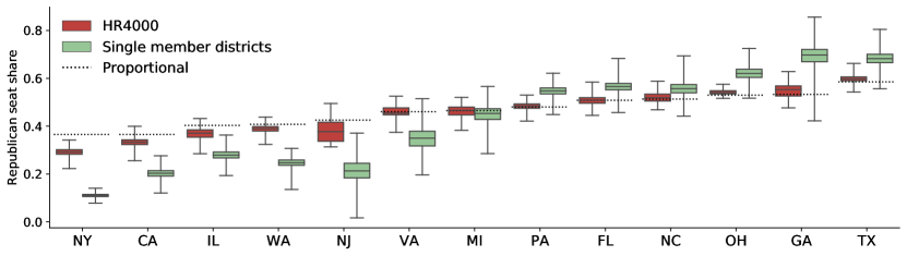
Figure 3: Comparison of Republican seat share distribution of H.R. 4000 compliant ensembles using STV/PAV voting rule to single-member district baseline for all states with 10 or more seats (see Appendix Figure 8 for additional voting rules).

Effect of social choice function.

Perhaps the most obvious takeaway is that using a Winner takes all procedure with MMDs, as was popular in the twentieth century and still in effect in some state legislatures, enables rampant gerrymandering at nearly all district sizes and should be avoided (in fact, while proportionality gaps with one large Winner takes all MMD in each state cancel out at the national level in Figure 1, as shown in Figure 2(a) they increase to close to the theoretical maximum with larger MMDs).

Our results also illustrate the differential effects of the Thiele design parameter $\lambda$, especially as a function of district size. As we increase the rate at which $\lambda$ decays in $i$ (i.e., as the difference $\lambda(i)-\lambda(i+1)$ increases), the corresponding Thiele rule more strongly results in legislatures that are equally composed of members of different groups, regardless of the size of the underlying group. Especially with even-member districts, then, such a rule leads to proportional representation when the parties are approximately equi-sized—even more so than does STV or PAV—at the cost of proportionality for settings with imbalanced party size. For example, consider the difference between the national-scale proportionality of Thiele squared in Figure 1, with the per-state proportionality gap in Figure 2, with two-member districts. More generally, our empirical framework may be helpful in complementing theoretical analysis of Thiele rules (see, e.g., Skowron [88]) in understanding the effect of the design parameter in a given real-world setting, given the actual distribution of voters.

District size design heterogeneity and recommendations.

Our discussion above suggests that two or three member districts (as possible depending on the number of seats) with STV or PAV would work well across most political conditions in the United States. In particular, fairness-minded independent commissions are able to achieve proportional outcomes in every state up to rounding, and advantage-minded partisans have their power to gerrymander significantly curtailed.

However, there is also important heterogeneity; individual states can further promote proportional outcomes by tuning MMD parameters based on their population, partisan lean, and political geography. See Appendix Figure 5 for full state-by-state results; here, we discuss the most relevant factors influencing ‘optimal’ district size. We observe that small and highly partisan states both benefit from larger districts. Smaller states have fewer opportunities for wasted votes to cancel out across districts and so can more easily become disproportionate. In contrast, highly partisan states often suffer from the ‘Massachusetts problem,’ where minority parties have difficulty breaking the requisite threshold in any district due to their diffuse voter base. In general, states with significant geographic self-segregation could protect the political power of both concentrated and diffuse voters with larger districts that inherently waste fewer surplus and losing votes.

As such, flexibility across states may be beneficial; however, as Figure 1 shows, such flexibility may also increase gerrymandering, if within a state partisan gerrymanderers can use a mixture of district sizes. We evaluate this trade-off by studying the potential outcomes of redistricting under H.R. 4000, a proposal mandating that the number of seats per district, $N_{k}\in\{3,4,5\}$. Figure 3 suggests that H.R. 4000. would allow flexibility without giving gerrymanderers too many degrees of freedom in district size: it enables proportionality almost everywhere, and it does not offer significant additional capacity to gerrymander over a baseline of using just three- or just five-member districts, in contrast to the case of mixing single- and two-member districts.

This finding is important because coherent communities substantially vary in size and so are best represented by variable sized districts. For instance, in Texas, the Houston metro area may be best served by a five-member district whereas, San Antonio, a city with roughly half the population, may best be served by a three-member district. Under a fixed number of seats per district, either Houston is split, or San Antonio is grouped together with disjoint communities. We believe H.R. 4000 strikes an effective balance. In the next section, we continue evaluating such trade-offs, studying intra-party effects of MMDs with STV, where the solid coalitions assumption no longer holds.

4 Results: Intra-party diversity

So far, we have studied how multi-member districts affect the balance of power between parties. However, one of the primary justifications of Rank Choice Voting (either for SMDs or MMDs) is that it enables minor parties or ideologies to gain seats – it blunts the game-theoretic logic that tends Winner takes all democracies toward two parties. In this section, we analyze such claims by showing the effects of MMDs on intra-party diversity.

The biggest challenge to studying such effects is that the solid coalitions assumption of 1 does not hold—there are substantial cross-over meaningful votes between coalitions within a party; we must now generate intra-party rankings and simulate STV. There is a further conceptual challenge: coalitions within parties are not well-defined, and identifying them with data is challenging; with many candidates, no two voters may share the same exact ballot preference order. In theory, results are often proven with regards to arbitrary-sized coalitions who approve the same candidates (cf. Skowron [88]), but relating the guarantees back to coalitions in practice is difficult; it is unclear who are the coalitions to which one should be proportional, especially with limited ranked choice data, and how exactly to define proportionality for these groups.

We leverage additional political structure to tackle these challenges. (1) First, instead of considering arbitrary coalitions, we examine voter rankings emerging from differing assumptions on how voters value two dimensions: (approximate) political preference, and geographic preference. We choose these dimensions since single-member districts automatically impose one dimension (geographic) as more important, while in theory MMDs allow voters to prefer political connection over geographic proximity. (2) Second, we measure intra-party effects through two measures: the diversity of the winning candidate set, and the diversity of the coalitions supporting each winner. If the former increases, then that means more distinct within-party preferences are represented by the winning set. If the latter increases, that means each particular winner is accountable to a more diverse intra-party voter base. However, we do not claim that these dimensions are the most important – our simulation provides a method to understand for how various dimensions trade off; insight for any given political setting requires careful consideration of the most important dimensions and their relationships. Rollout of MMDs might further affect partisan behavior and relationships, making it challenging to study such effects precisely before an implementation.

4.1 Methods and assumptions

To study the case when the solid coalitions assumption is broken, we first need to construct plausible intra-party voter rankings and candidate distributions; second, we need to simulate STV elections given a map. For space reasons, methodological details are deferred to Section C.2.

Constructing intra-party rankings.

We require further assumptions on how voters differentially rank candidates within their party, to study how MMDs may change the characteristics of winners within a party. The key challenge is to develop a model for how a voter – given their characteristics – will vote given a menu of (hypothetical) candidates. Up to now, we have only assumed that voters approve all candidates of their party or rank them all above members of the other party.

We do so as follows, using the voter file described in Section 2.3. Recall that we have individual-level voter data in each block, along with demographic information and ideological scores; in particular we use the voter’s geographic location and a univariate partisan score indicating the strength of their party affiliation (most Republican to most Democratic). We generate many synthetic candidates for each party in each district, with varying demographic information and partisan scores; the distribution of candidates reflects that of the voters. Finally, we assume that—while voters still rank all same-party candidates over other-party candidates—within each party they rank candidates in order of the distance between their characteristics (either partisan scores or geographic location, in different simulations). As a result, solid coalitions no longer holds within parties, where voter preferences may not be expressed neatly in terms of sub-parties.

We note that while there has been much work on spatial voter models aiming to characterize such behavior based on the “distance” between the voter and each candidate [2, 93, 86, 66], it is a hard challenge – it is not clear that voters behave according to such ideological spatial positioning, beyond the relative consistency of party membership. Thus, our results should not be interpreted as what would necessarily happen with multi-member districts, but what intra-party coalitions could or could not be formed with MMDs given voter interest, and how these coalitions differ from those possible under SMDs.

Running STV elections.

Given the candidates, sampled voters, and the voters’ rankings over the candidates, we run fractional STV for each district in each given map. We do so for the random, neutral maps calculated above, as we wish to study intra-party effects as distinct from partisan ones. Running these STV elections utilized over 60 CPU-weeks of compute, on top of the map generation discussed in Section 2.3. This run-time is for given maps, underscoring the necessity of 1 to study partisan seat shares without needing to simulate STV during the redistricting optimization process.

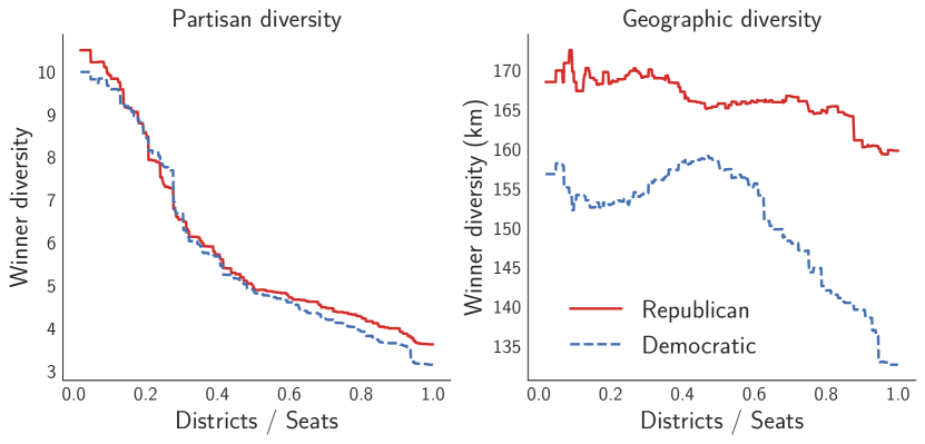
(a) Diversity of winning candidate set

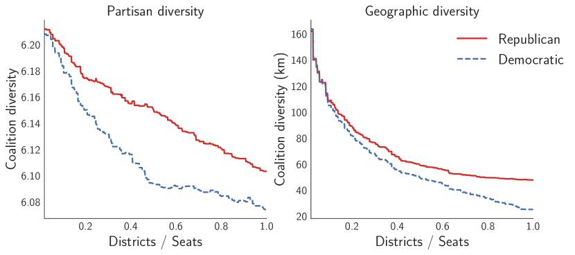
(b) Diversity of coalitions supporting winners

Figure 4: How intra-party diversity measures vary with the number of districts. (a) The diversity of the winning candidate set. (b) The diversity of the voters who supported a given winning candidate, averaged by party. These results establish that, with STV, a more diverse set of winners can be elected, i.e., minority viewpoints within a party are supported. Simultaneously, each winning candidate draws support from a more diverse coalition of voters.

4.2 Results

Figure 4 contains our intra-party results, when we assume that within a party voters rank according to partisan score. First, Figure 4(a) illustrates how MMDs affect the diversity of the winning set within each party. For each map, we determine the set of winners for each party and then calculate the standard deviation of their partisan scores. For geographic diversity, we calculate the average Euclidean distance of each winner from the centroid of the winners’ locations. We find that with STV and large districts, a more diverse set of winners emerge, within each party. The intuition for partisan score is simple and is similar to that regarding diffusion of minority party voters across a state (the Massachusetts problem). When voters rank according to partisan score, then similar voters across the state can pool their votes to ensure that a favored candidate wins. Using SMDs, these voters may be split across different districts, such that in each a different intra-party coalition chooses the winning candidate. Surprisingly, larger districts simultaneously increase the geographic diversity of winners, even when voters rank according to partisan score.

Second, Figure 4(b) shows that with MMDs each winning candidate draws support from a more diverse coalition of voters. For each winner, we determine the voters who contributed votes in the STV round in which the candidate was elected, weighted by how many votes they provided (since we do fractional STV). For partisan score, we calculate the (weighted) standard deviation of the partisan scores of the voter coalition. For geographic diversity, we calculate the (weighted) average voter euclidean distance from the district centroid. Finally, we average across winners within each party.

This result establishes that MMDs may come at a cost, in terms of the geographic representation aspect of our representative democracy: insofar as it is valuable for a representative to be accountable to a geographically cohesive set of voters (such as for providing constituent services or acquire funding for projects), large MMDs weaken such ties; voter coalitions move from about 25 kilometers from the coalition center on average to almost 160 kilometers. Two- or three-member districts, however, come at a far smaller cost.

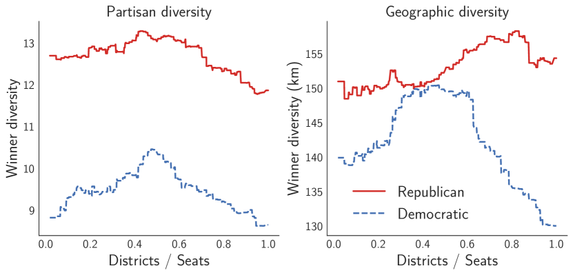
(a) Diversity of winning candidate set

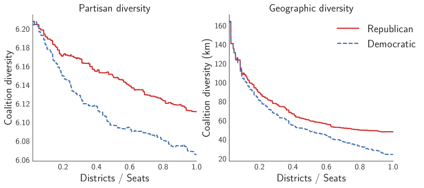
(b) Diversity of coalitions supporting each winner

Figure 10: Same as Figure 4, except voters now rank within party based on geographic distance.

Appendix Figure 10 contains the same plots when voters’ intra-party rank is according to geography. Perhaps as expected, under this assumption MMDs do not increase the diversity of the winners according to partisan scores – if voters do not band together based on partisan scores, then their mutually preferred candidates on this dimension do not win. However, the findings regarding coalition diversity remains virtually identical: even when voters rank within a party based on geographical distance to a candidate, each winner represents a far more geographically dispersed coalition than with SMDs.

While this finding may seem paradoxical, it can occur when party members are not evenly distributed throughout the state – whereas members in a (smaller) city may with SMDs be big enough to elect a preferred member, in MMDs they may be over-ruled by a larger group of same-party members in another city. This finding adds a warning to the notion of proportionality—small, potentially intersectionally defined groups may be better served by small districts, even as theoretical proportionality guarantees monotonically increase in district size. Most practically for the United States, more research is needed on the effect of MMDs on minority voters (cf. Benade et al. [21]).

Overall, our results caution in choosing too big a district size for MMDs, especially as our results in Section 3 suggest that most of the proportionality benefits can be achieved with two- or three-member districts—and results in this section suggest that such districts come at a smaller cost in terms of geographic cohesiveness. More broadly, this section gives an approach to evaluating the effects of voting rules and redistricting on intra-party outcomes, by generating various voter rankings from individual-level data and then studying the effects with respect to interpretable dimensions.

5 Discussion

Discussion and Limitations

In this work, we focus empirically on the United States and on MMDs. There are many other systems designed for proportionality in use internationally; a comparative study would be of use. Furthermore, other places also use MMDs – in Singapore, for example, the ruling party has been accused of using MMDs with Winner takes all rules to gerrymander (with boundaries determined immediately before the election) [97]. Future work also should adopt our methodology to study partisan gerrymandering in state and local legislatures, especially in the states that already use (Winner takes all) MMDs. Such legislatures stand to benefit even more from MMDs than congressional districts given that they cannot rely on interstate cancellation of partisan bias as is currently the case in the House of Representatives. While we expect the high level insights to hold, details may differ when zooming in with more seats in a smaller region due to, e.g., effects of geography.

There is much left to do to understand multi-member districts in practice, especially how it relates to other constraints and laws. (1) The 2021 version of H.R. 4000 has a provision that MMDs should not be used in states where doing so would violate the Voting Rights Act; it would be crucial to analyze under what circumstances this could happen and how one would measure violations. (2) More generally, we impose no constraints beyond contiguity and population balance, but many areas impose additional requirements (such as minimizing the splitting of county boundaries). (3) We assume that voters rank all candidates, when in practice there may be “ballot exhaust.” We note that our main results shows the effectiveness of two- and three-member districts, where voters may be more likely to submit full rankings. Cataloging and computationally enforcing such constraints and features is a challenging; we conjecture that adding such features from practice is important but will have second-order effects. Also crucial is studying how intra-party effects such as those studied in Section 4 (and in the work of, e.g., Angulu et al. [4] and Buck et al. [26]) interact with partisan gerrymandering (or gerrymandering on other characteristics).

Conclusion.

We study the joint gerrymandering and social choice problem, showing the promise of multi-member districts with non-Winner takes all rules in ensuring partisan proportionality, in terms of both enabling independent commissions and constraining partisan gerrymanders. We show that H.R. 4000 achieves an ideal balance between flexibility of representation while ensuring proportionality. Finally, while this work is empirical, it raises many theoretical questions that we expect to be of interest to the computational social choice community. For example, while much is known about proportionality in the case of one large MMD (see, e.g., Skowron [88] and references therein), to our knowledge no work has considered it in the case of multiple MMDs. Our results suggest that under party-based voting, the proportionality gap decreases (non-monotonically) with district size; showing this effect under more general assumptions, including how it interacts with the intra-party effects highlighted in Section 4, is of interest.

Appendix A Supplementary results

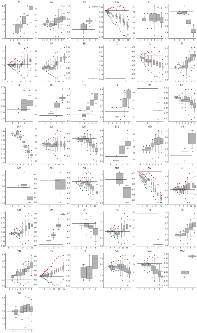
Figure 5: Figure 2(b), repeated for each state with at least 2 Representatives. Y-Axis is Republican seat share.

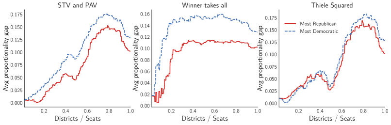
Figure 6: Proportionality gap in favor of each party in most advantageous map

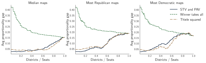
Figure 7: Figure 2(a), repeated for Median, Most Republican, and Most Democratic maps.

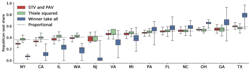
Figure 8: Seat share distribution of H.R. 4000 compliant ensemble by voting rule.

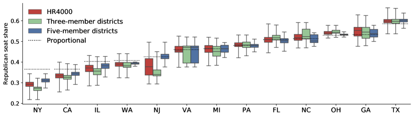
Figure 9: Comparison of Republican seat share distribution of H.R. 4000 compliant ensembles with baseline for all states with 10 or more seats using STV/PAV voting rule (see Appendix Figure 8 for more rules). H.R. 4000 mandates $N_{k}\in\{3,4,5\}$. The baseline is to use only three-member and only five-member districts (with four-member districts for overflow as necessary).

Figure 5 shows the complete state-by-state results for STV based elections where the high level patterns from Figure 1 can be seen in more granular details. For example the bump structure at uniform district sizes is very clear for Michigan (MI), Flordia (FL), Wisconsin (WI), California (CA), North Carolina (NC), and Pennsylvania (PA), among others. In CA, MA, NY, OK, and TN single-member proportional plans are not even possible due to the diffusion of minority party voters. In all states, the maximum gerrymandering capability peaks at about 1.5 seats per district and starts to decay rapidly with larger districts.

In Figure 6 we see that, under full control of the redistricting process, Democrats could actually more effectively gerrymander the House of Representatives than Republicans, a finding counter to the conventional wisdom that geography favors Republican gerrymandering [34, 24]. The main caveat, is that this analysis is still using only "natural" districts – those which aren’t wildly contorted – and therefore does not include the most surgical gerrymanders. This is a standard challenge in redistricting algorithms, which are effective for large-scale analysis but can often be out-performed (with respect to any metric) in any specific setting by experts. Regardless, as shown in Figure 5, it is true that Democrats can gerrymander their large states (CA, NY, and IL) more effectively than Republicans can gerrymander theirs (TX and FL), and that when ignoring the VRA, Democrats can crack large cities into many Democratically leaning wedge-shaped districts. Furthermore, the gap in advantage is largest at two- and three-member districts because these thresholds enable Democrats to more efficiently place their voters than Republicans. For STV in particular, Democrats can break the $\frac{2}{3}$ or $\frac{3}{4}$ threshold needed for a sweep in many urban districts, while also still clearing the $\frac{1}{3}$ or $\frac{1}{4}$ threshold needed to gain one seat in rural districts, resulting in fewer wasted votes across most types of districts. While critics might point to this as a deal-breaker, it is important to recognize that this is only true in the limit of Democratic control, and such a scenario is deeply unrealistic.

In Figure 7, we show how the median, max Republican, and max Democratic absolute proportionality gap changes as a function of the voting rule and ratio of districts to seats. The median gap drops by about a factor of three between single-member and two-member districts and continues to slowly decay with larger districts. The median gap is a relevant metric because it proxies how easy it is to create a proportional map. Similarly, if the median map is fair, then there exists many fair maps, and it becomes easier to optimize for other desirable criteria like proportional racial representation, maintaining political subdivisions, and compactness. Also in Figure 7, we see that STV and Thiele squared track each other very closely, with the exception of Democratic gerrymanders of two- and three-member districts. This follows similar logic as the overall Democratic advantage analysis above, except that because Thiele squared requires more votes for a sweep, Democrats can no longer rely on full control of districts with just above $\frac{2}{3}$ of votes, and so end up wasting many votes in more heavily democratic areas by just missing the sweep threshold.

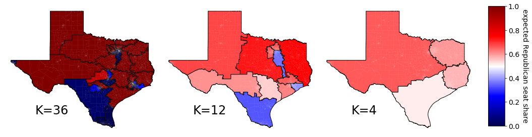
Figure 11: Example fair multi-member plans for Texas.

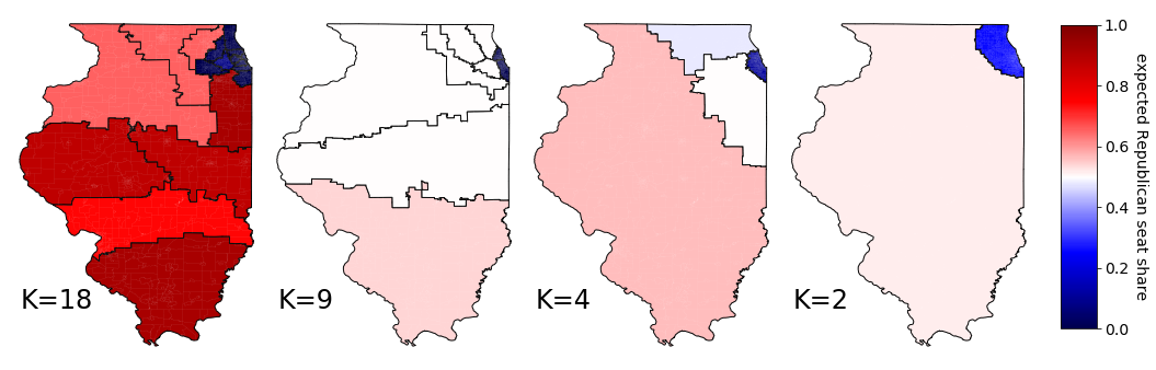
Figure 12: Example fair multi-member plans for Illinois.

Appendix B Proofs

Lemma B.1.

Consider

$$n_{R}(y_{R},\lambda_{PAV})=\min_{n}\left[\operatorname*{arg\,max}_{n}\left[y_{R}\sum_{i=1}^{n}\lambda(i)+(1-y_{R})\sum_{i=1}^{M-n}\lambda(i)\right]\right].$$

and let $n_{R}(y_{R},STV)$ be the unique integer such that

$$y_{R}(M+1)-1\leq n_{R}(y_{R},STV)<y_{R}(M+1)$$

Then, $n_{R}(y_{R},\lambda_{\text{PAV}})=n_{R}(y_{R},STV)$, for all $y_{R},M$.

Proof.

We have that $n_{R}(y_{R},\lambda_{PAV})$ is $n$ such that:

$$n\geq 1\implies y_{R}\lambda(n)>(1-y_{R})\lambda(M-n+1)$$

$$n<M\implies y_{R}\lambda(n+1)\leq(1-y_{R})\lambda(M-n)$$

The first condition requires that choosing the $n$th candidate from party R is strictly (due to tie-breaking against R) more valuable than choosing the ($M-n+1$)th candidate from party D.

The second condition requires that choosing the ($n+1$)th candidate from party R is no more valuable than choosing the ($M-n$)th candidate from party D.

Rewriting the first condition, we have

$$n\geq 1\implies\frac{y_{R}}{n} >\frac{1-y_{R}}{M-n+1}$$

$$\iff\frac{y_{R}}{n}+\frac{y_{R}}{M-n+1} >\frac{1}{M-n+1}$$

$$\iff\frac{y_{R}(M+1)}{n(M-n+1)} >\frac{1}{M-n+1}$$

$$\iff\frac{y_{R}}{n} >\frac{1}{(M+1)}$$

Similarly, rewriting the second condition yields

$$n<M\implies\frac{y_{R}}{n+1} \leq\frac{1}{(M+1)}$$

∎

See 1

Proof.

The first part of the result is known [94, 49]. For completeness, we provide a proof using our notation and in our exact setting.

For expositional simplicity, we assume that $V\text{ mod }(M+1)=0$, i.e., the number of votes is evenly divisible by one plus the number of winners, though the same arguments extend. Then, let $Q=\left\lfloor\frac{V}{M+1}\right\rfloor+1=\frac{V}{M+1}+1$ be the Droop quota.

To understand the intuition, note that the given seat shares would immediately hold if each party had a coordinator who could optimally decide how voters of that party rank candidates within the party. In that case, the coordinator would ensure that as many candidates as possible have first place votes equal to the Droop quota, with no first place votes going to candidates who will be eliminated. The resulting seat shares follow, given tie-breaking against party R (and, if needed, the surplus vote transfer procedure for the additional single vote needed in the Droop quota).

However, this argument is not sufficient because, in principle, candidates could receive meaningful votes from voters of the other party. Further, without such a coordinator, sub-optimal arrangement of votes could potentially lead to elimination of candidates who would be elected with such a coordinator. (The former reason is fundamental, and is why the exact formula does not hold in general without parties or even for more than 2 parties without further assumptions; the latter possibility is exactly the issue that STV surplus vote transfers are designed to avoid, and eliminating it is book-keeping). The proof centers around eliminating these two possibilities.

The key step in the proof is noting that under the assumptions, that votes can only transferred from a candidate of one party to a candidate of the other party (either after a candidate is eliminated or selected as a winner) if candidates from the sender party have been exhausted, as the sender party voters rank all other party members after all their own party members.

Thus, for any set of voter rankings under the assumptions, the per-party seat share remains the same under re-arrangements of how each voter ranks members of the other party (at the point that such rearrangements matter for who is elected, only one party candidates are left, and so the partisan seat share does not change). Thus, without loss of generality, for the rest of the proof we assume that all voters within a party share the same ordering for candidates of the other party.

Recall that the Droop quota is designed such that no more than $M$ total candidates can ever meet the Droop quota across rounds. Doing so would require at least $M(Q-1)+Q$ total votes (as votes necessary to reach the quota minus 1 are never transferred and so not double counted, and the $(M+1)$th candidate would require $Q$ votes), and

$$M(Q-1)+Q =M\left[\frac{V}{M+1}\right]+\left[\frac{V}{M+1}+1\right]$$

$$=V+1>V$$

The above facts establish that we can carry out the initial rounds of STV separately for each party, until in each party there are either no candidates remaining or all remaining candidates for that party have votes exactly equal to $Q-1$: no votes are transferred across parties up to this stage; as long as we only elect candidates with votes at or above the Droop Quota, we do not mistakenly elect any candidate separately that we would not have together; and if this stage is ever reached, the identities of the elected or eliminated candidates does not matter, since up to now there is a conservation of votes by party and so the per-party counts remain the same.

Now, consider each party $p$, and suppose in current round that $W_{p}$ candidates have been elected for the party. Further suppose that there are $m_{p}\geq 1$ candidates left for the party, and they have $q_{p}=y_{p}V-(W_{p})(Q-1)$ number of first place votes (either original first place votes, or votes after transfers) among them. If $q_{p}\geq(Q-1)m_{p}$ and there exists a candidate with vote share not exactly $Q-1$, then by the pigeonhole principle, there exists at least one candidate of the party such that the votes for that candidate meets the Droop quota $Q$ and is selected. Then, that candidate is declared a winner, and its surplus votes are transferred to other candidates of the same party. Then, iterate with $W_{p}+1$, $m_{p}-1$, and $q_{p}-(Q-1)$. Otherwise, eliminate the candidate in the party with the least number of votes, and iterate with $m_{p}-1$ and $q_{p}$ until $m_{p}=0$ or the remaining candidates all have a number of votes equal to $Q-1$.

Suppose at the end of these separate processes, $W_{p}$ candidates from each party have been elected, and there are $T_{p}$ candidates tied with $(Q-1)$ votes each. We know that $y_{p}V\geq(W_{p}+T_{p})(Q-1)$, as at least this many votes were required to elect $W_{p}$ candidates and have the remaining tied at $Q-1$.

Thus,

$$n_{p}(y_{p},STV) \leq(W_{p}+T_{p})$$ Other candidates eliminated

$$\leq\frac{y_{p}V}{Q-1}$$

$$=y_{p}(M+1)$$

Furthermore, $n_{R}(y_{R},STV)+n_{D}(y_{D},STV)=M$, and so for each party $p\neq s$, we have

$$n_{p}(y_{p},STV) =M-n_{s}(y_{s},STV)$$

$$\geq M-y_{s}(M+1)$$

$$=M-(1-y_{p})(M+1)$$

$$=M-M-1+y_{p}(M+1)=y_{p}(M+1)-1$$

Next, note that the inequality $n_{p}(y_{p},STV)\leq y_{p}(M+1)$ is strict for party $R$, given the tie-breaking favoring party $D$ by assumption: either $T_{R}=0$ and so $W_{R}<\frac{y_{R}V}{Q-1}$ (the last candidate selected had votes at or above $Q$), or there is a tie involving a candidate of party $R$ who does not get selected, $n_{R}(y_{R},STV)<(W_{R}+T_{R})$.

The proof is finished by applying Lemma B.1.

∎

Appendix C Empirical methodological detail

C.1 Map Generation

All details of the original Stochastic Hierarchical Partitioning (SHP) algorithm can be found in the paper by Gurnee and Shmoys [61] and associated appendices; we further use their same geographic and electoral data (see Appendix Table 2 of Gurnee and Shmoys [61]). Here, we discuss the relevant algorithmic parameters and differences from that. We plan to make our github public.

Multi-member.

The main algorithmic difference from the original SHP algorithm is that we adapted ours to generate multi-member districts. To do this, instead of parameterizing a sample tree node by a region $R$ and total number of seats $s$, we needed to also specify the number of districts that node contains. This is required because at an intermediate node, the number of districts is not immediately derivable from the total number of seats in that node because of ambiguity in the number of $N_{k}$ versus $N_{k}+1$ sized districts. Therefore, the number of seats is used just to balance population, and the number of districts is used for all other tree operations (sampling valid splits, maintaining balance, etc.).

Ensembles.

For each pair (state, $K$), with $K\in\{2,3,\dots,10,12,\dots,20,23,\dots 53\}\cup\{N\}$ and $K\leq N$, we sampled the root node $\left(\frac{1000}{K}\right)^{1.2}$ times and each internal node $\left(\frac{300}{K}\right)^{0.5}$ times. These constants were chosen to balance computational cost and optimization quality. We used random-iterative center selection with Voronoi-weighted capacity matching to sample region centers and sizes. All districts are population balanced within a $1\%$ tolerance. Each of these ensembles were then scored, optimized, and subsampled to create a final distribution over partisan outcomes.

C.2 Intra-party method details

Here, we provide additional detail for Section 4.

Voter multi-dimensional preferences

In the voter file provided to us, each voter is assigned scores on a variety of ideological and demographic dimensions, including party preference those on specific issues. See the following blog post for additional details on these scores, under “Survey-based machine learning support scores”: https://predictwise.medium.com/what-all-we-did-for-the-2020-elections-78b66a44f651. Here we use the partisan score value, which is an overall score from 0 to 100 designed to represent how likely a voter is to lean Democrat in the two-party vote; this score is derived from party registration, past primary voting data, demographic information, etc. As the post shows, this score well-correlates with issue-preference scores. We threshold this value; above the threshold, a voter is declared a Democrat and below the threshold, a Republican.

As a second dimension, we use geography – based on the voter’s home location; for computational simplicity and privacy reasons, we use the centroid of the census block in which the voter’s home location resides, as opposed to the latitude/longitude information of the voter.

Candidate generation

Next, we generate one candidate for each (party, census block) combination as follows. (Results do not change with multiple candidates for each (party, census block) combination). The home address of the candidate is taken to be the centroid of the census block. The partisan score of the candidate is taken to be the median partisan score of voters in the corresponding party in that block.

Voters and candidates in an election

Recall – from the map generation stage – that a given map is a partition of the census tracts into districts. Note that each voter and candidate belongs to a census block, and thus a unique district in each map.

In a given election (as characterized by the map, social choice function, and number of winners in each district), each voter has available to them a subset of the candidates (those belonging to a census block in the same district as the voter). The method to generate candidates might produce many candidates or voters in a given district (e.g., if the district makes up the entire state); for computational reasons, we sample at most 5000 voters and 1000 candidates from each district.

Turning voter preferences into rankings

In each simulated election, we need a ranking over candidates from each voter. These are generated as follows. First, as in the assumption of 1, we assume that each voter ranks their own party candidates over all other-party candidates. Within each party, voters rank candidates according to a distance function. As introduced in Section 4, for some settings we assume that the distance function is first determined by the partisan score – voters rank candidates according to the absolute value of the difference of their partisan scores, with ties if any broken by geography. In other settings, we assume that the distance function is determined first by geography, with voters preferring closer candidates according to the Euclidean distance between the latitude/longitude associated with each voter and candidate (and ties broken by partisan score). Unlike reality, we assume that there is no ballot exhaust – these simulated voters submit complete rankings.

Simulating STV elections

From the above steps, for each election in each district, we have a set of candidates and voters who have submitted rankings over the candidates. (Up to 5000 voters and 1000 candidates). We run fractional STV for each such district.

This entire process took over 60 CPU-weeks to compute for all the setting, with the largest computational load being generating the individual voter rankings and then running fractional STV.

References

- [1]
- Adams et al. [2017] James Adams, Erik Engstrom, Danielle Joeston, Walt Stone, Jon Rogowski, and Boris Shor. 2017. Do Moderate Voters Weigh Candidates’ Ideologies? Voters’ Decision Rules in the 2010 Congressional Elections. Political Behavior 39, 1 (March 2017), 205–227. https://doi.org/10.1007/s11109-016-9355-7
- American Academy of Arts and Sciences [2020] American Academy of Arts and Sciences. 2020. Our Common Purpose: Reinventing American Democracy for the 21st Century. https://www.amacad.org/sites/default/files/publication/downloads/2020-Democratic-Citizenship_Our-Common-Purpose_0.pdf
- Angulu et al. [2019] Hakeem Angulu, Ruth Buck, Daryl DeFord, Moon Duchin, Howard Fain, Max Hully, Maira Khan, Zach Schutzman, and Oliver York. 2019. Study of Reform Proposals for Chicago City Council. https://mggg.org/Chicago.pdf
- Ansolabehere and Rodden [2011a] Stephen Ansolabehere and Jonathan Rodden. 2011a. Alabama Data Files. https://doi.org/10.7910/DVN/UUCWPP
- Ansolabehere and Rodden [2011b] Stephen Ansolabehere and Jonathan Rodden. 2011b. Indiana Data Files. https://doi.org/10.7910/DVN/WYXFW3
- Ansolabehere and Rodden [2011c] Stephen Ansolabehere and Jonathan Rodden. 2011c. Mississippi Data Files. https://doi.org/10.7910/DVN/AN00LH
- Ansolabehere and Rodden [2011d] Stephen Ansolabehere and Jonathan Rodden. 2011d. New Jersey Data Files. https://doi.org/10.7910/DVN/KX0YGR
- Ansolabehere and Rodden [2011e] Stephen Ansolabehere and Jonathan Rodden. 2011e. New York Data Files. https://doi.org/10.7910/DVN/AWE39N
- Arrow et al. [2010] Kenneth J Arrow, Amartya Sen, and Kotaro Suzumura. 2010. Handbook of Social Choice and Welfare. Vol. 2. Elsevier.
- Autry et al. [2020] Eric A Autry, Daniel Carter, Gregory Herschlag, Zach Hunter, and Jonathan C Mattingly. 2020. Multi-scale merge-split Markov chain Monte Carlo for redistricting. arXiv preprint arXiv:2008.08054 (2020).
- Autry et al. [2021] Eric A Autry, Daniel Carter, Gregory J Herschlag, Zach Hunter, and Jonathan C Mattingly. 2021. Metropolized Multiscale Forest Recombination for Redistricting. Multiscale Modeling & Simulation 19, 4 (2021), 1885–1914.
- Aziz et al. [2017] Haris Aziz, Markus Brill, Vincent Conitzer, Edith Elkind, Rupert Freeman, and Toby Walsh. 2017. Justified Representation in Approval-Based Committee Voting. Social Choice and Welfare 48, 2 (Feb. 2017), 461–485. https://doi.org/10.1007/s00355-016-1019-3
- Aziz et al. [2015] Haris Aziz, Serge Gaspers, Joachim Gudmundsson, Simon Mackenzie, Nicholas Mattei, and Toby Walsh. 2015. Computational Aspects of Multi-Winner Approval Voting. In Proceedings of the 2015 International Conference on Autonomous Agents and Multiagent Systems (AAMAS ’15). International Foundation for Autonomous Agents and Multiagent Systems, Richland, SC, 107–115. http://dl.acm.org/citation.cfm?id=2772879.2772896
- Bachrach et al. [2016] Yoram Bachrach, Omer Lev, Yoad Lewenberg, and Yair Zick. 2016. Misrepresentation in District Voting.. In IJCAI. 81–87.
- Balinski and Young [2010] Michel L Balinski and H Peyton Young. 2010. Fair representation: meeting the ideal of one man, one vote. Brookings Institution Press.
- Ballotpedia [2021a] Ballotpedia. 2021a. Arizona State Legislature. https://ballotpedia.org/Arizona_State_Legislature
- Ballotpedia [2021b] Ballotpedia. 2021b. State legislative chambers that use multi-member districts. https://ballotpedia.org/State_legislative_chambers_that_use_multi-member_districts
- Banzhaf [1966] John F. Banzhaf. 1966. Multi-Member Electoral Districts. Do They Violate the "One Man, One Vote" Principle. The Yale Law Journal 75, 8 (July 1966), 1309. https://doi.org/10.2307/795047
- Becker et al. [2020] Amariah Becker, Moon Duchin, Dara Gold, and Sam Hirsch. 2020. Computational Redistricting and the Voting Rights Act. (2020), 54.
- Benade et al. [2021a] Gerdus Benade, Ruth Buck, Moon Duchin, Dara Gold, and Thomas Weighill. 2021a. Ranked Choice Voting and Minority Representation. SSRN Scholarly Paper ID 3778021. Social Science Research Network, Rochester, NY. https://doi.org/10.2139/ssrn.3778021
- Benade and Procaccia [2020] Gerdus Benade and Ariel Procaccia. 2020. Abating gerrymandering by mandating fairness. Preprint (2020).
- Benade et al. [2021b] Gerdus Benade, Ariel Procaccia, and Jamie Tucker-Foltz. 2021b. You can have your cake and redistrict it too. ACM Transactions on Economics and Computation (2021).
- Borodin et al. [2018] Allan Borodin, Omer Lev, Nisarg Shah, and Tyrone Strangway. 2018. Big City vs. the Great Outdoors: Voter Distribution and How It Affects Gerrymandering.. In IJCAI. 98–104.
- Brandt et al. [2016] Felix Brandt, Vincent Conitzer, Ulle Endriss, Jérôme Lang, and Ariel D Procaccia. 2016. Handbook of Computational Social Choice. Cambridge University Press.
- Buck et al. [2019] Ruth Buck, Moon Duchin, Dara Gold, and JN Matthews. 2019. Community-Centered Redistricting in Lowell, Massachusetts. https://mggg.org/uploads/Lowell-Report.pdf
- Bullock III [1989] Charles S Bullock III. 1989. Symbolics or Substance: A Critique of the at-Large Election Controversy. State & Local Government Review (1989), 91–99.
- Bullock III and Gaddie [1993] Charles S Bullock III and Ronald Keith Gaddie. 1993. Changing from multimember to single-member districts: partisan, racial, and gender consequences. State & Local Government Review (1993), 155–163.
- Cannon et al. [2020] Sarah Cannon, Ari Goldbloom-Helzner, Varun Gupta, JN Matthews, and Bhushan Suwal. 2020. Voting Rights, Markov Chains, and Optimization by Short Bursts. arXiv preprint arXiv:2011.02288 (2020).
- Caragiannis et al. [2017] Ioannis Caragiannis, Swaprava Nath, Ariel D. Procaccia, and Nisarg Shah. 2017. Subset Selection via Implicit Utilitarian Voting. Journal of Artificial Intelligence Research 58 (Jan. 2017), 123–152. https://doi.org/10.1613/jair.5282
- Cembrano et al. [2021b] Javier Cembrano, Jose Correa, Gonzalo Diaz, and Victor Verdugo. 2021b. Proportional Apportionment: A Case Study From the Chilean Constitutional Convention. In Equity and Access in Algorithms, Mechanisms, and Optimization. 1–9.
- Cembrano et al. [2021a] Javier Cembrano, José Correa, and Victor Verdugo. 2021a. Multidimensional Apportionment through Discrepancy Theory. Available at SSRN 3864480 (2021).
- Chatterjee and DasGupta [2019] Tanima Chatterjee and Bhaskar DasGupta. 2019. On partisan bias in redistricting: computational complexity meets the science of gerrymandering. arXiv preprint arXiv:1910.01565 (2019).
- Chen and Rodden [2013] Jowei Chen and Jonathan Rodden. 2013. Unintentional gerrymandering: Political geography and electoral bias in legislatures. Quarterly Journal of Political Science 8, 3 (2013), 239–269.
- Cheng et al. [2019] Yu Cheng, Zhihao Jiang, Kamesh Munagala, and Kangning Wang. 2019. Group Fairness in Committee Selection. In Proceedings of the 2019 ACM Conference on Economics and Computation (EC ’19). Association for Computing Machinery, New York, NY, USA, 263–279. https://doi.org/10.1145/3328526.3329577
- Chikina et al. [2017] Maria Chikina, Alan Frieze, and Wesley Pegden. 2017. Assessing significance in a Markov chain without mixing. Proceedings of the National Academy of Sciences 114, 11 (2017), 2860–2864.
- Conitzer and Xia [2012] Vincent Conitzer and Lirong Xia. 2012. Paradoxes of Multiple Elections: An Approximation Approach.. In KR. Citeseer.
- Data and Lab [2018] MIT Election Data and Science Lab. 2018. County Presidential Election Returns 2000-2016. https://doi.org/10.7910/DVN/VOQCHQ
- Dauer [1966] Manning J. Dauer. 1966. Multi-Member Districts in Dade County: Study of a Problem and a Delegation. The Journal of Politics 28, 3 (Aug. 1966), 617–638. https://doi.org/10.2307/2128159
- Davidson and Korbel [1981] Chandler Davidson and George Korbel. 1981. At-Large Elections and Minority-Group Representation: A Re-Examination of Historical and Contemporary Evidence. The Journal of Politics 43, 4 (Nov. 1981), 982–1005. https://doi.org/10.2307/2130184
- DeFord and Duchin [2019] Daryl DeFord and Moon Duchin. 2019. Redistricting reform in Virginia: Districting criteria in context. Virginia Policy Review 12, 2 (2019), 120–146.
- DeFord et al. [2020] Daryl DeFord, Moon Duchin, and Justin Solomon. 2020. A Computational Approach to Measuring Vote Elasticity and Competitiveness. Statistics and Public Policy just-accepted (2020), 1–30.
- DeFord et al. [2021] Daryl DeFord, Moon Duchin, and Justin Solomon. 2021. Recombination: A Family of Markov Chains for Redistricting. Harvard Data Science Review (31 3 2021). https://doi.org/10.1162/99608f92.eb30390f https://hdsr.mitpress.mit.edu/pub/1ds8ptxu.
- Derfner [1972] Armand Derfner. 1972. Multi-Member Districts and Black Voters. The Black Law Journal 2 (1972), 120.
- Dewan and Shepsle [2011] Torun Dewan and Kenneth A. Shepsle. 2011. Political Economy Models of Elections. Annual Review of Political Science 14, 1 (June 2011), 311–330. https://doi.org/10.1146/annurev.polisci.12.042507.094704
- Duchin [2018] Moon Duchin. 2018. Outlier analysis for Pennsylvania congressional redistricting.
- Duchin et al. [2019] Moon Duchin, Taissa Gladkova, Eugene Henninger-Voss, Ben Klingensmith, Heather Newman, and Hannah Wheelen. 2019. Locating the representational baseline: Republicans in Massachusetts. Election Law Journal: Rules, Politics, and Policy 18, 4 (2019), 388–401.
- Duchin et al. [2020] Moon Duchin, Tom Needham, and Thomas Weighill. 2020. The (Homological) Persistence of Gerrymandering. arXiv:2007.02390 [physics] (July 2020). arXiv:2007.02390 [physics] http://arxiv.org/abs/2007.02390
- Dummett [1984] Michael Dummett. 1984. Voting procedures. (1984).
- Elkind et al. [2017] Edith Elkind, Piotr Faliszewski, Jean-François Laslier, Piotr Skowron, Arkadii Slinko, and Nimrod Talmon. 2017. What do multiwinner voting rules do? An experiment over the two-dimensional euclidean domain. In Proceedings of the AAAI Conference on Artificial Intelligence, Vol. 31.
- Elkind et al. [2015] Edith Elkind, Piotr Faliszewski, Piotr Skowron, and Arkadii Slinko. 2015. Properties of Multiwinner Voting Rules. arXiv:1506.02891 [cs] (June 2015). arXiv:1506.02891 [cs] http://arxiv.org/abs/1506.02891
- Erikson [1972] Robert S Erikson. 1972. Malapportionment, gerrymandering, and party fortunes in congressional elections. The American Political Science Review (1972), 1234–1245.
- Ernst [1994] Lawrence R Ernst. 1994. Appointment methods for the House of Representatives and the court challenges. Management Science 40, 10 (1994), 1207–1227.
- FairVote [2017] FairVote. 2017. The Fair Representation Act. https://www.fairvote.org/fair_rep_in_congress
- FairVote [2021] FairVote. 2021. Details about Ranked Choice Voting. https://www.fairvote.org/rcv
- Faliszewski et al. [2019] Piotr Faliszewski, Piotr Skowron, Stanisław Szufa, and Nimrod Talmon. 2019. Proportional representation in elections: STV vs PAV. In Proceedings of the 18th International Conference on Autonomous Agents and MultiAgent Systems. 1946–1948.
- Fifield et al. [2020] Benjamin Fifield, Michael Higgins, Kosuke Imai, and Alexander Tarr. 2020. Automated redistricting simulation using Markov chain Monte Carlo. Journal of Computational and Graphical Statistics 29, 4 (2020), 715–728.
- Garg et al. [2019] Nikhil Garg, Lodewijk L Gelauff, Sukolsak Sakshuwong, and Ashish Goel. 2019. Who Is in Your Top Three? Optimizing Learning in Elections with Many Candidates. In Proceedings of the AAAI Conference on Human Computation and Crowdsourcing, Vol. 7. 22–31.
- Gerber et al. [1998] Elisabeth R. Gerber, Rebecca B. Morton, and Thomas A. Rietz. 1998. Minority Representation in Multimember Districts. American Political Science Review 92, 1 (March 1998), 127–144. https://doi.org/10.2307/2585933
- Grose [2020] Christian R. Grose. 2020. Reducing Legislative Polarization: Top-Two and Open Primaries Are Associated with More Moderate Legislators. Journal of Political Institutions and Political Economy 1, 2 (2020), 267–287. https://doi.org/10.1561/113.00000012
- Gurnee and Shmoys [2021] Wes Gurnee and David B Shmoys. 2021. Fairmandering: A column generation heuristic for fairness-optimized political districting. Proceedings of the 2021 SIAM Conference on Applied and Computational Discrete Algorithms (ACDA21) (2021). https://doi.org/10.1137/1.9781611976830.9
- Hamilton [1967] Howard D. Hamilton. 1967. Legislative Constituencies: Singe-Member Districts, Multi-Member Districts, and Floterial Districts. The Western Political Quarterly 20, 2 (1967), 321–340. https://doi.org/10.2307/445408
- Herschlag et al. [2020] Gregory Herschlag, Han Sung Kang, Justin Luo, Christy Vaughn Graves, Sachet Bangia, Robert Ravier, and Jonathan C Mattingly. 2020. Quantifying gerrymandering in north carolina. Statistics and Public Policy 7, 1 (2020), 30–38.
- Herschlag et al. [2017] Gregory Herschlag, Robert Ravier, and Jonathan C Mattingly. 2017. Evaluating partisan gerrymandering in Wisconsin. arXiv preprint arXiv:1709.01596 (2017).
- Issacharoff [2002] Samuel Issacharoff. 2002. Gerrymandering and political cartels. Harv. L. Rev. 116 (2002), 593.
- Jessee [2009] Stephen A. Jessee. 2009. Spatial Voting in the 2004 Presidential Election. American Political Science Review 103, 1 (Feb. 2009), 59–81. https://doi.org/10.1017/S000305540909008X
- King et al. [2015] Douglas M King, Sheldon H Jacobson, and Edward C Sewell. 2015. Efficient geo-graph contiguity and hole algorithms for geographic zoning and dynamic plane graph partitioning. Mathematical Programming 149, 1-2 (2015), 425–457.
- Klain [1955] Maurice Klain. 1955. A New Look at the Constituencies: The Need for a Recount and a Reappraisal. American Political Science Review 49, 4 (1955), 1105–1119.
- Kueng et al. [2019] Richard Kueng, Dustin G Mixon, and Soledad Villar. 2019. Fair redistricting is hard. Theoretical Computer Science 791 (2019), 28–35.
- Lackner and Skowron [2018] Martin Lackner and Piotr Skowron. 2018. A Quantitative Analysis of Multi-Winner Rules. arXiv:1801.01527 [cs] (Jan. 2018). arXiv:1801.01527 [cs] http://arxiv.org/abs/1801.01527
- Lempert [2021] Benjamin P Lempert. 2021. Ranked-Choice Voting as Reprieve from the Court-Ordered Map. Michigan Law Review 119, 8 (2021), 1785–1818.
- Liu et al. [2016] Yan Y Liu, Wendy K Tam Cho, and Shaowen Wang. 2016. PEAR: a massively parallel evolutionary computation approach for political redistricting optimization and analysis. Swarm and Evolutionary Computation 30 (2016), 78–92.
- McCartan and Imai [2020] Cory McCartan and Kosuke Imai. 2020. Sequential Monte Carlo for sampling balanced and compact redistricting plans. arXiv preprint arXiv:2008.06131 (2020).
- McDaniel [2018] Jason McDaniel. 2018. Does More Choice Lead to Reduced Racially Polarized Voting? Assessing the Impact of Ranked-Choice Voting in Mayoral Elections. California Journal of Politics and Policy 10, 2 (2018). https://doi.org/10.5070/P2cjpp10241252
- McGann et al. [2016] Anthony J McGann, Charles Anthony Smith, Michael Latner, and Alex Keena. 2016. Gerrymandering in America: The House of Representatives, the Supreme Court, and the future of popular sovereignty. Cambridge University Press.
- McGhee and Shor [2017] Eric McGhee and Boris Shor. 2017. Has the Top Two Primary Elected More Moderates? Perspectives on Politics 15, 4 (Dec. 2017), 1053–1066. https://doi.org/10.1017/S1537592717002158
- MGGG [2020] MGGG. 2020. MGGG States. https://github.com/mggg-states.
- MGGG Redistricting Lab [2022] MGGG Redistricting Lab. 2022. Modeling the Fair Representation Act.
- Niemi et al. [1985] Richard G. Niemi, Jeffrey S. Hill, and Bernard Grofman. 1985. The Impact of Multimember Districts on Party Representation in U. S. State Legislatures. Legislative Studies Quarterly 10, 4 (1985), 441–455. https://doi.org/10.2307/440068
- Niemi et al. [1991] Richard G. Niemi, Simon Jackman, and Laura R. Winsky. 1991. Candidacies and Competitiveness in Multimember Districts. Legislative Studies Quarterly 16, 1 (1991), 91–109. https://doi.org/10.2307/439969
- Page and Gilens [2018] Benjamin I. Page and Martin Gilens. 2018. Making American Democracy Representative. https://prospect.org/power/making-american-democracy-representative/
- Pegden et al. [2017] Wesley Pegden, Ariel D Procaccia, and Dingli Yu. 2017. A partisan districting protocol with provably nonpartisan outcomes. arXiv preprint arXiv:1710.08781 (2017).
- Pukelsheim [2017] Friedrich Pukelsheim. 2017. Proportional representation. Springer.
- Puppe and Tasnádi [2008] Clemens Puppe and Attila Tasnádi. 2008. A computational approach to unbiased districting. Mathematical and Computer Modelling 48, 9-10 (2008), 1455–1460.
- Rogowski and Langella [2015] Jon C. Rogowski and Stephanie Langella. 2015. Primary Systems and Candidate Ideology: Evidence from Federal and State Legislative Elections. American Politics Research 43, 5 (Sept. 2015), 846–871. https://doi.org/10.1177/1532673X14555177
- Shor and Rogowski [2018] Boris Shor and Jon C. Rogowski. 2018. Ideology and the US Congressional Vote. Political Science Research and Methods 6, 2 (April 2018), 323–341. https://doi.org/10.1017/psrm.2016.23
- Silva [1964] Ruth C Silva. 1964. Compared Values of the Single-and the Multi-Member Legislative District. Western Political Quarterly 17, 3 (1964), 504–516.
- Skowron [2019] Piotr Skowron. 2019. Proportionality Degree of Multiwinner Rules. arXiv:1810.08799 [cs] (Oct. 2019). arXiv:1810.08799 [cs] http://arxiv.org/abs/1810.08799
- Spencer et al. [2015] Andrew Spencer, Christopher Hughes, and Rob Richie. 2015. Escaping the Thicket: The Ranked Choice Voting Solution to America’s Redistricting Crisis. Cumberland Law Review 46, 2 (2015), 377–424. https://heinonline.org/HOL/P?h=hein.journals/cumlr46&i=389
- Stephanopoulos and McGhee [2015] Nicholas O Stephanopoulos and Eric M McGhee. 2015. Partisan gerrymandering and the efficiency gap. U. Chi. L. Rev. 82 (2015), 831.
- Still [1991] Edward Still. 1991. Voluntary Constituencies: Modified at-Large Voting as a Remedy for Minority Vote Dilution in Judicial Elections Overview: Electoral Reform. Yale Law & Policy Review 9, 2 (1991), 354–369. https://heinonline.org/HOL/P?h=hein.journals/yalpr9&i=362
- Swamy et al. [2019] Rahul Swamy, Douglas King, and Sheldon Jacobson. 2019. Multi-Objective Optimization for Political Districting: A Scalable Multilevel Approach. (2019), 26.
- Tausanovitch and Warshaw [2018] Chris Tausanovitch and Christopher Warshaw. 2018. Does the Ideological Proximity between Candidates and Voters Affect Voting in U.S. House Elections? Political Behavior 40, 1 (March 2018), 223–245. https://doi.org/10.1007/s11109-017-9437-1
- Tideman [1995] Nicolaus Tideman. 1995. The single transferable vote. Journal of Economic Perspectives 9, 1 (1995), 27–38.
- Trounstine and Valdini [2008] Jessica Trounstine and Melody E. Valdini. 2008. The Context Matters: The Effects of Single-Member versus at-Large Districts on City Council Diversity. American Journal of Political Science 52, 3 (2008), 554–569. https://doi.org/10.1111/j.1540-5907.2008.00329.x
- Tucker-Foltz [2018] Jamie Tucker-Foltz. 2018. A Cut-And-Choose Mechanism to Prevent Gerrymandering. arXiv preprint arXiv:1802.08351 (2018).
- Tung [2020] Ngiam Shih Tung. 2020. How Gerrymandering Creates Unfair Elections in Singapore. New Naratif (2020). https://newnaratif.com/how-gerrymandering-creates-unfair-elections-in-singapore/
- Voting and Election Science Team [2018] Voting and Election Science Team. 2018. 2016 Precinct-Level Election Results. https://doi.org/10.7910/DVN/NH5S2I
- Voting and Election Science Team [2019] Voting and Election Science Team. 2019. 2018 Precinct-Level Election Results. https://doi.org/10.7910/DVN/UBKYRU
- Walawender [1985] Richard A. Walawender. 1985. At-Large Elections and Vote Dilution: An Empirical Study Symposium: Environmental Law: Note. University of Michigan Journal of Law Reform 19, 4 (1985), 1221–1242. https://heinonline.org/HOL/P?h=hein.journals/umijlr19&i=1231
- Wang [2016] Samuel S-H Wang. 2016. Three tests for practical evaluation of partisan gerrymandering. Stan. L. Rev. 68 (2016), 1263.
- Warrington [2018] Gregory S Warrington. 2018. Quantifying gerrymandering using the vote distribution. Election Law Journal 17, 1 (2018), 39–57.