Distributed Dual Subgradient Methods with Averaging and Applications to Grid Optimization

Haitian Liu  Subhonmesh Bose  Hoa Dinh Nguyen
Ye Guo  Thinh T. Doan  Carolyn L. Beck
S. Bose and C.L. Beck are with the University of Illinois at Urbana-Champaign, Urbana, IL 61801, USA. H.D. Nguyen is with the International Institute for Carbon-Neutral Energy Research (WPI-I2CNER) and Institute of Mathematics for Industry (IMI), Kyushu University, 744 Motooka, Nishi-ku, Fukuoka 819-0395, Japan. H. Liu and Y. Guo are with the Tsinghua-Berkeley Shenzhen Institute, Shenzhen, Guangdong 518055, China. T.T. Doan is with Virginia Tech, Blacksburg, VA 24060 USA. E-mails: boses@illinois.edu, hoa.nd@i2cner.kyushu-u.ac.jp, liuht19@mails.tsinghua.edu.cn, guo-ye@sz.tsinghua.edu.cn, thinhdoan@vt.edu, beck3@illinois.edu. This project was partially supported by grants from the Power Systems Engineering Research Center (PSERC), JSPS Kakenhi Grant Number JP23K03906, National Science Foundation of China under Grant 51977115.
Abstract

We study finite-time performance of a recently proposed distributed dual subgradient (DDSG) method for convex constrained multi-agent optimization problems. The algorithm enjoys performance guarantees on the last primal iterate, as opposed to those derived for ergodic means for vanilla DDSG algorithms. Our work improves the recently published convergence rate of 𝒪(logT/T)𝒪𝑇𝑇{\cal O}(\log T/\sqrt{T}) with decaying step-sizes to 𝒪(1/T)𝒪1𝑇{\cal O}(1/\sqrt{T}) with constant step-size on a metric that combines suboptimality and constraint violation. We then numerically evaluate the algorithm on three grid optimization problems. Namely, these are tie-line scheduling in multi-area power systems, coordination of distributed energy resources in radial distribution networks, and joint dispatch of transmission and distribution assets. The DDSG algorithm applies to each problem with various relaxations and linearizations of the power flow equations. The numerical experiments illustrate various properties of the DDSG algorithm–comparison with vanilla DDSG, impact of the number of agents, and why Nesterov-style acceleration can fail in DDSG settings.

1 Introduction

Distributed optimization algorithms offer mechanisms to optimize in multi-agent environments, where one cannot aggregate all problem data in a central location. Agents in this paradigm iteratively perform local computational steps and communicate relevant variables over a network. While a variety of distributed solution architectures have been developed and analyzed in the literature for various settings, we focus on distributed dual subgradient (DDSG) methods with averaging that can be used to solve convex constrained multi-agent optimization problems of the form

𝒫::𝒫absent\displaystyle{\cal P}:\ minimize𝒙1,,𝒙Nsubscript𝒙1subscript𝒙𝑁minimize\displaystyle\underset{{\bm{x}}_{1},\ldots,{\bm{x}}_{N}}{\text{minimize}} j=1Nfj(𝒙j),superscriptsubscript𝑗1𝑁subscript𝑓𝑗subscript𝒙𝑗\displaystyle\quad\sum_{j=1}^{N}f_{j}({\bm{x}}_{j}), (1a)
subject to j=1N𝒈jE(𝒙j)=0,superscriptsubscript𝑗1𝑁superscriptsubscript𝒈𝑗Esubscript𝒙𝑗0\displaystyle\quad\sum_{j=1}^{N}{\bm{g}}_{j}^{\textrm{E}}({\bm{x}}_{j})=0, (1b)
j=1N𝒈jI(𝒙j)0,superscriptsubscript𝑗1𝑁superscriptsubscript𝒈𝑗Isubscript𝒙𝑗0\displaystyle\quad\sum_{j=1}^{N}{\bm{g}}_{j}^{\textrm{I}}({\bm{x}}_{j})\leq 0, (1c)
𝒙j𝕏jnj,j=1,,N.formulae-sequencesubscript𝒙𝑗subscript𝕏𝑗superscriptsubscript𝑛𝑗𝑗1𝑁\displaystyle\quad{\bm{x}}_{j}\in\mathds{X}_{j}\subseteq\mathds{R}^{n_{j}},\ j=1,\ldots,N. (1d)

The N𝑁N agents communicate only across edges of an undirected graph 𝔊(N,𝔼)𝔊𝑁𝔼{\mathfrak{G}}(N,\mathds{E}). Assume that functions fjsubscript𝑓𝑗f_{j}, 𝒈jIsuperscriptsubscript𝒈𝑗I{\bm{g}}_{j}^{\textrm{I}} are convex and 𝒈jEsuperscriptsubscript𝒈𝑗E{\bm{g}}_{j}^{\textrm{E}} is affine over the compact convex set 𝕏jsubscript𝕏𝑗\mathds{X}_{j} for each j=1,,N𝑗1𝑁j=1,\ldots,N.

At its core, DDSG methods rely on dual decomposition that starts by separating the Lagrangian into agent-wise Lagrangian functions that each agent optimizes, given a dual iterate (see classical texts such as [3, 32]). This agent-wise optimization of the primal variables, given a dual iterate, can be shown to provide a subgradient of the dual function at the dual iterate. Thus, a subgradient ascent on the dual function can be achieved to solve the dual problem. Such an update rule requires a central coordinator to manage the dual iterates, which is undesirable in many distributed contexts. DDSG methods circumvent this need by maintaining local copies of such multipliers and running a consensus-based distributed dual ascent on these local multiplier copies. Approximate primal solutions can be recovered from these dual solutions as in [34], building on techniques in [27, 16, 24, 20], among others; asymptotic guarantees on recovered primal sequences are also known.

In this paper, we study a distributed dual subgradient method, analyzed recently in [22], that provides a fully distributed variant of the algorithm, also proposed recently in [30]. As opposed to vanilla DDSG algorithms, convergence guarantees of these algorithms are obtained for the last primal iterate as opposed to that for ergodic means of primal sequences. As Nesterov and Shikhman argue in [30], iterates in vanilla DDSG algorithms can oscillate wildly during algorithm execution. If the intermediate primal iterates of the algorithm are implemented in practice, vanilla DDSG can negatively impact stability in multi-agent environments. Besides, primal recovery is no longer required for asymptotic constraint satisfaction in this paradigm.

For the algorithms in [22, 30], asymptotic guarantees for the convergence of the last primal-dual iterate to the set of primal-dual optimizers have been established with decaying step-sizes. Also, the authors of [22] characterize a 𝒪(logT/T)𝒪𝑇𝑇{\cal O}(\log T/\sqrt{T})-bound on a metric that combines sub-optimality and constraint violation with decaying step-size (similar to [12]), while they argue a lower bound of 𝒪(1/T)𝒪1𝑇{\cal O}(1/\sqrt{T}). Their analysis shows an 𝒪(1/T)𝒪1𝑇{\cal O}(1/\sqrt{T})-bound, when a coordinator manages the dual updates centrally. Thus, they view the logT𝑇\log T factor as a price for decentralization. Our first contribution of this paper is to close this gap in Section 2 with the proof in Section 3, i.e., we sharpen the convergence rate to 𝒪(1/T)𝒪1𝑇{\cal O}(1/\sqrt{T}) for this fully distributed algorithm with a constant step-size. The dual function for 𝒫𝒫{\cal P} can be nonsmooth, and as a result, a first-order algorithm that climbs the dual function cannot converge at a better rate (see Appendix A), making the algorithm order-optimal.

Through the rest of the paper, we study various properties of our DDSG algorithm on 𝒫𝒫{\cal P}. Specifically, we consider three different optimization problems that arise in operations of the electric power system and cast them as examples of 𝒫𝒫{\cal P}. For each problem, we adopt different power flow models, different notions of agents and different definitions of the network over which these agents interact. This exercise stands as our second contribution, which demonstrates the modeling power of 𝒫𝒫{\cal P} and the broad applicability of the algorithm with convergence guarantees. The grid optimization problems are nonconvex due to the nature of Kirchhoff’s laws [9]. In this paper, we convexify each problem by considering approximations and convex relaxations for power flow models that are suited to that application. Each problem and the application of DDSG illustrates specific properties of the algorithm that are delineated below.

\bullet Multi-area optimal power flow (𝒫1subscript𝒫1{\cal P}_{1}) seeks to dispatch resources over an interconnected transmission network, parts of which are controlled by different system operators. The distributed algorithmic architecture we study in Section 4, bypasses the need for the system operators to share all relevant data from within their footprint with another system operator and yet seek to solve a joint optimal power flow problem through a distributed solution architecture, e.g., see [15]. For 𝒫1subscript𝒫1{\cal P}_{1}, we consider a linear power flow model for transmission networks motivated by the use of such models in wholesale market environments that facilitate inter-area coordination, e.g., in [35]. Through the numerical example on 𝒫1subscript𝒫1{\cal P}_{1}, we demonstrate how the averaging scheme stabilizes the last iterate, compared to vanilla DDSG methods, and circumvents the need for primal recovery. We also show that finite-time constraint violation of the algorithm is empirically better than its theoretical bound suggests.

\bullet Coordination of distributed energy resources (DERs) in distribution grids (𝒫2subscript𝒫2{\cal P}_{2}) is designed to optimize real and reactive power outputs from DERs at the grid-edge to minimize cost (dis-utility) of such a dispatch and possibly a network-wide objective such as frequency regulation. A distributed algorithm allows quick updates of optimization variables without the need to communicate with a central coordinator across the distribution grid. For 𝒫2subscript𝒫2{\cal P}_{2} in Section 5, we consider a second-order cone programming (SOCP) based relaxation of the power flow equations in the distribution grids. The thoroughly-studied SOCP-based relaxation of power flow equations for distribution grids are often tight in practice (see [13, 14]). Through examples of 𝒫2subscript𝒫2{\cal P}_{2}, we show that our algorithm can track changing grid conditions for small networks. Tracking performance degrades with network size, where aggregation of nodes as agents becomes vital for performance. Said differently, if speed is paramount, one must carefully control the degree of decentralization.

\bullet Transmission and distribution (T&D) grid coordination (𝒫3subscript𝒫3{\cal P}_{3}) seeks to dispatch assets across the transmission and distribution grids without the need to collect all information from the grid-edge and the bulk power systems at one location. The distributed solution architecture in Section 6 alleviates the transmission system operator’s lack of visibility into utility-managed distribution networks. For 𝒫3subscript𝒫3{\cal P}_{3}, we consider two different power flow models for the transmission and the distribution grids. For transmission, we choose a semidefinite programming (SDP) based relaxation of power flow equations, given its popularity to approach the AC optimal power flow problem [21, 37, 5]. For the distribution grids, we consider the linear distribution power flow model from [1]. Using an example of 𝒫3subscript𝒫3{\cal P}_{3}, we compare the empirical performance of the DDSG method with an adopted distributed acceleration scheme proposed in [33], where acceleration fails to increase convergence speed with linear costs, but performs well with quadratic costs. We argue that nonsmoothness of the dual function with linear costs is behind this phenomenon, and elaborate on its role in Appendix A.

We recognize that a long literature has emerged on each of the grid optimization problems; we only cite a few, owing to space constraints. Our goal in presenting the power system examples is not an attempt to empirically compare our DDSG algorithm with others in the literature proposed for these problems. Rather, our formulations of these problems as instances of 𝒫𝒫{\cal P} reveal the generality of 𝒫𝒫{\cal P} and make it possible for subsequent unified algorithm development for 𝒫𝒫{\cal P}. In addition, each example highlights an important aspect of the DDSG algorithm.

2 The dual subgradient method with averaging

We present the DDSG algorithm to solve 𝒫𝒫{\cal P} in (1). The finite-time performance guarantee for 𝒫𝒫{\cal P} is derived in Section 3. Then in Sections 4, 5 and 6, we cast 𝒫1subscript𝒫1{\cal P}_{1}, 𝒫2subscript𝒫2{\cal P}_{2} and 𝒫3subscript𝒫3{\cal P}_{3} as examples of 𝒫𝒫{\cal P}.

To lighten notation, let 𝒈jsubscript𝒈𝑗{\bm{g}}_{j} collect both 𝒈jEsuperscriptsubscript𝒈𝑗E{\bm{g}}_{j}^{\textrm{E}} and 𝒈jIsuperscriptsubscript𝒈𝑗I{\bm{g}}_{j}^{\textrm{I}} with the understanding that the first MEsuperscript𝑀EM^{\textrm{E}} constraints encode equalities and the last MIsuperscript𝑀IM^{\textrm{I}} are inequalities. The algorithm relies on Lagrangian duality theory associated with 𝒫𝒫{\cal P}. We begin by defining the Lagrangian function

(𝒙,𝒛):=j=1N[fj(𝒙j)+𝒛𝒈j(𝒙j)],𝒙𝒛assignabsentsuperscriptsubscript𝑗1𝑁delimited-[]subscript𝑓𝑗superscript𝒙𝑗superscript𝒛subscript𝒈𝑗subscript𝒙𝑗\displaystyle\begin{aligned} {\cal L}({\bm{x}},{\bm{z}})&:=\sum_{j=1}^{N}\left[f_{j}({\bm{x}}^{j})+{\bm{z}}^{{\mathchoice{\raisebox{0.75346pt}{$\displaystyle\intercal$}}{\raisebox{0.75346pt}{$\textstyle\intercal$}}{\raisebox{0.75346pt}{$\scriptstyle\intercal$}}{\raisebox{0.75346pt}{$\scriptscriptstyle\intercal$}}}}{\bm{g}}_{j}({\bm{x}}_{j})\right],\end{aligned} (2)
𝒙=(𝒙1,,𝒙NT)𝕏:=𝕏1××𝕏N,𝒛:=ME×+MI.formulae-sequencesuperscript𝒙superscriptsubscript𝒙1superscriptsubscript𝒙𝑁𝑇𝕏assignsubscript𝕏1subscript𝕏𝑁𝒛assignsuperscriptsuperscript𝑀Esubscriptsuperscriptsuperscript𝑀I\displaystyle\begin{gathered}{\bm{x}}^{\mathchoice{\raisebox{0.75346pt}{$\displaystyle\intercal$}}{\raisebox{0.75346pt}{$\textstyle\intercal$}}{\raisebox{0.75346pt}{$\scriptstyle\intercal$}}{\raisebox{0.75346pt}{$\scriptscriptstyle\intercal$}}}=({\bm{x}}_{1}^{\mathchoice{\raisebox{0.75346pt}{$\displaystyle\intercal$}}{\raisebox{0.75346pt}{$\textstyle\intercal$}}{\raisebox{0.75346pt}{$\scriptstyle\intercal$}}{\raisebox{0.75346pt}{$\scriptscriptstyle\intercal$}}},\ldots,{\bm{x}}_{N}^{T})\in\mathds{X}:=\mathds{X}_{1}\times\ldots\times\mathds{X}_{N},\\ {\bm{z}}\in\mathds{Z}:=\mathds{R}^{M^{\textrm{E}}}\times\mathds{R}^{M^{\textrm{I}}}_{+}.\end{gathered} (5)

Then, 𝒫𝒫{\cal P} can be cast as a min-max problem with optimal value 𝒫superscript𝒫{\cal P}^{\star} as

𝒫=min𝒙𝕏max𝒛(𝒙,𝒛).superscript𝒫subscript𝒙𝕏subscript𝒛𝒙𝒛\displaystyle{{\cal P}}^{\star}=\min_{{\bm{x}}\in\mathds{X}}\max_{{\bm{z}}\in\mathds{Z}}\ {\cal L}({\bm{x}},{\bm{z}}). (6)

Let 𝕏superscript𝕏\mathds{X}^{\star} denote the set of optimizers of 𝒫𝒫{\cal P}. Associated with 𝒫𝒫{\cal P} is its dual problem

𝒫D=max𝒛min𝒙𝕏(𝒙,𝒛).superscriptsubscript𝒫𝐷subscript𝒛subscript𝒙𝕏𝒙𝒛\displaystyle{\cal P}_{D}^{\star}=\max_{{\bm{z}}\in\mathds{Z}}\min_{{\bm{x}}\in\mathds{X}}\ {\cal L}({\bm{x}},{\bm{z}}). (7)

Let superscript\mathds{Z}^{\star} denote the set of optimizers of the dual problem. Weak duality implies that 𝒫𝒫Dsuperscript𝒫superscriptsubscript𝒫𝐷{\cal P}^{\star}\geq{\cal P}_{D}^{\star}. We say strong duality holds if the inequality is met with an equality. And, 𝒙𝕏superscript𝒙𝕏{\bm{x}}^{\star}\in\mathds{X}, 𝒛superscript𝒛{\bm{z}}^{\star}\in\mathds{Z} is a saddle point of {\cal L}, if

(𝒙,𝒛)(𝒙,𝒛)(𝒙,𝒛),superscript𝒙𝒛superscript𝒙superscript𝒛𝒙superscript𝒛\displaystyle{\cal L}({\bm{x}}^{\star},{\bm{z}})\leq{\cal L}({\bm{x}}^{\star},{\bm{z}}^{\star})\leq{\cal L}({\bm{x}},{\bm{z}}^{\star}), (8)

for all 𝒙𝕏,𝒛formulae-sequence𝒙𝕏𝒛{\bm{x}}\in\mathds{X},{\bm{z}}\in\mathds{Z}. The well-known saddle point theorem (see [4, Theorem 2.156]) states that the primal-dual optimizers 𝕏×superscript𝕏superscript\mathds{X}^{\star}\times\mathds{Z}^{\star} coincide with the saddle points of {\cal L}. We assume throughout that the set of saddle points of 𝒫𝒫{\cal P} is nonempty and bounded. As a result, strong duality holds for 𝒫𝒫{\cal P}, i.e., 𝒫=𝒫Dsuperscript𝒫superscriptsubscript𝒫𝐷{\cal P}^{\star}={\cal P}_{D}^{\star}, and the set of primal-dual optimizers is nonempty. Saddle-points exist under standard constraint qualifications such as Slater’s condition, e.g., see [4, Theorem 2.165].

Dual decomposition techniques for distributed optimization rely on the observation that the dual function separates into agent-wise optimization problems, given a multiplier 𝒛𝒛{\bm{z}} as

min𝒙𝕏(𝒙,𝒛)=j=1Nmin𝒙j𝕏jj(𝒙j,𝒛):=𝒟j(𝒛),subscript𝒙𝕏𝒙𝒛superscriptsubscript𝑗1𝑁subscriptsubscriptsubscript𝒙𝑗subscript𝕏𝑗subscript𝑗subscript𝒙𝑗𝒛assignabsentsubscript𝒟𝑗𝒛\displaystyle\min_{{\bm{x}}\in\mathds{X}}\ {\cal L}({\bm{x}},{\bm{z}})=\sum_{j=1}^{N}\underbrace{\min_{{\bm{x}}_{j}\in\mathds{X}_{j}}{\cal L}_{j}({\bm{x}}_{j},{\bm{z}})}_{:={\cal D}_{j}({\bm{z}})}, (9)

where j(𝒙j,𝒛):=fj(𝒙j)+𝒛𝒈j(𝒙j)assignsubscript𝑗subscript𝒙𝑗𝒛subscript𝑓𝑗superscript𝒙𝑗superscript𝒛subscript𝒈𝑗subscript𝒙𝑗{\cal L}_{j}({\bm{x}}_{j},{\bm{z}}):=f_{j}({\bm{x}}^{j})+{\bm{z}}^{{\mathchoice{\raisebox{0.75346pt}{$\displaystyle\intercal$}}{\raisebox{0.75346pt}{$\textstyle\intercal$}}{\raisebox{0.75346pt}{$\scriptstyle\intercal$}}{\raisebox{0.75346pt}{$\scriptscriptstyle\intercal$}}}}{\bm{g}}_{j}({\bm{x}}_{j}). If the agents can perform these agent-wise minimizations, then a distributed projected subgradient ascent algorithm can solve the dual problem (e.g., see [7]). Per Danskin’s theorem, a subgradient 𝒛𝒟j(𝒛)subscript𝒛subscript𝒟𝑗𝒛\nabla_{\bm{z}}{\cal D}_{j}({\bm{z}}) can be obtained from the agent-wise minimization of jsubscript𝑗{\cal L}_{j}, given that the sub-differential set of the concave function 𝒟jsubscript𝒟𝑗{\cal D}_{j} at 𝒛𝒛{\bm{z}} is

z𝒟j(𝒛):=conv{zj(𝒙j,𝒛)𝒙j𝕏j(𝒛)}.assignsubscript𝑧subscript𝒟𝑗𝒛convconditional-setsubscript𝑧subscript𝑗subscript𝒙𝑗𝒛subscript𝒙𝑗superscriptsubscript𝕏𝑗𝒛\displaystyle\partial_{z}{\cal D}_{j}({\bm{z}}):=\textrm{conv}\{\partial_{z}{\cal L}_{j}({\bm{x}}_{j},{\bm{z}})\ \mid\ {\bm{x}}_{j}\in\mathds{X}_{j}^{\star}({\bm{z}})\}. (10)

Here, “conv” computes the convex hull of its argument and 𝕏j(𝒛)superscriptsubscript𝕏𝑗𝒛\mathds{X}_{j}^{\star}({\bm{z}}) is the set of minimizers of j(,𝒛)subscript𝑗𝒛{\cal L}_{j}(\cdot,{\bm{z}}) over 𝕏jsubscript𝕏𝑗\mathds{X}_{j}. The minimization problem is well-defined, given that 𝕏jsubscript𝕏𝑗\mathds{X}_{j}’s are compact. Running such an algorithm, however, requires a central coordinator to compute the 𝒛𝒛{\bm{z}}-update and broadcast the results to all agents. Albeit simpler than aggregating all problem data at a single location, the need for said coordination is a downside of classical dual decomposition.

To avoid coordination for the dual update, one can alternately create local copies of 𝒛𝒛{\bm{z}}’s among all agents and enforce equality among these local estimates in the dual problem as

maxj=1N𝒟j(𝒛j),subject to 𝒛j=𝒛k,j,k=1,,N,formulae-sequencesuperscriptsubscript𝑗1𝑁subscript𝒟𝑗subscript𝒛𝑗subject to subscript𝒛𝑗subscript𝒛𝑘𝑗𝑘1𝑁\displaystyle\begin{aligned} \max\ \sum_{j=1}^{N}{\cal D}_{j}({\bm{z}}_{j}),\text{subject to }{\bm{z}}_{j}={\bm{z}}_{k},\ j,k=1,\ldots,N,\end{aligned} (11)

where 𝒛jsubscript𝒛𝑗{\bm{z}}_{j} is the local copy of 𝒛𝒛{\bm{z}} with agent j𝑗j. One can run a projected distributed subgradient ascent as in [34] to solve (11). The primal iterates obtained from agent-wise minimization of jsubscript𝑗{\cal L}_{j} evaluated at the dual iterates may fail to collectively satisfy the constraints of 𝒫𝒫{\cal P}. Primal averaging schemes have been studied in [34]; limit points of such recovered primal solutions are known to satisfy the constraints. One can judiciously maintain local copies only among a subset of the agents to relieve communication burden (see [18]).

Recently, a dual subgradient algorithm was proposed in [30] that leveraged an estimation sequence technique to provide guarantees on sub-optimality and infeasibility on the last iterate. This algorithm does not treat ergodic means simply as outputs from a dual subgradient calculation, but rather uses these means as primal-dual iterates to run the algorithm. We focus on the fully distributed variant of the algorithm that is proposed and analyzed in [22]. To present the algorithm, let 𝑾N×N𝑾superscript𝑁𝑁{\bm{W}}\in\mathds{R}^{N\times N} be a doubly stochastic, irreducible and aperiodic weighting matrix that follows the sparsity pattern of 𝔊𝔊{\mathfrak{G}}, i.e.,

Wj,k0(j,k)𝔼.iffsubscript𝑊𝑗𝑘0𝑗𝑘𝔼\displaystyle W_{j,k}\neq 0\iff(j,k)\in\mathds{E}. (12)

Then, the distributed projected dual subgradient with averaging is given by Algorithm 1, where 𝒙j/𝑿jsubscript𝒙𝑗subscript𝑿𝑗{\bm{x}}_{j}/{\bm{X}}_{j} are primal sequences and 𝒛j/𝒁jsubscript𝒛𝑗subscript𝒁𝑗{\bm{z}}_{j}/{\bm{Z}}_{j} are dual sequences. The updates comprise minimization of the local dual function in step 1, averaging of these primal minimizers in step 1, a consensus followed by local subgradient-based dual update in step 1 and an ergodic mean computation for the projected dual variable in step 1 with step-size η𝜂\eta. Here, πsubscriptπ{\uppi}_{\mathds{Z}} projects the arguments on \mathds{Z}.

1
2Choose 𝒛j(1)=0subscript𝒛𝑗10{\bm{z}}_{j}(1)=0, 𝒁j(0)=0subscript𝒁𝑗00{\bm{Z}}_{j}(0)=0, 𝒙j(0)𝕏jsubscript𝒙𝑗0subscript𝕏𝑗{\bm{x}}_{j}(0)\in\mathds{X}_{j} and η=η0/T𝜂subscript𝜂0𝑇\eta=\eta_{0}/\sqrt{T}.
3for t=1,,T𝑡1𝑇t=1,\ldots,T do
4      
5      𝑿j(t)argmin𝒙j𝕏jj(𝒙j,𝒛j(t))subscript𝑿𝑗𝑡subscriptargminsubscript𝒙𝑗subscript𝕏𝑗subscript𝑗subscript𝒙𝑗subscript𝒛𝑗𝑡{\bm{X}}_{j}(t)\leftarrow\mathop{\rm argmin}_{{\bm{x}}_{j}\in\mathds{X}_{j}}\ {\cal L}_{j}({\bm{x}}_{j},{\bm{z}}_{j}(t)).
6      𝒙j(t)t1t𝒙j(t1)+1t𝑿j(t)subscript𝒙𝑗𝑡𝑡1𝑡subscript𝒙𝑗𝑡11𝑡subscript𝑿𝑗𝑡{\bm{x}}_{j}(t)\leftarrow\frac{t-1}{t}{\bm{x}}_{j}(t-1)+\frac{1}{t}{\bm{X}}_{j}(t).
7      𝒁j(t)k=1NWjk𝒁k(t1)+t𝒈j(𝒙j(t))(t1)𝒈j(𝒙j(t1))subscript𝒁𝑗𝑡superscriptsubscript𝑘1𝑁subscript𝑊𝑗𝑘subscript𝒁𝑘𝑡1𝑡subscript𝒈𝑗subscript𝒙𝑗𝑡𝑡1subscript𝒈𝑗subscript𝒙𝑗𝑡1{\bm{Z}}_{j}(t)\leftarrow\sum_{k=1}^{N}W_{jk}{\bm{Z}}_{k}(t-1)+t{\bm{g}}_{j}({\bm{x}}_{j}(t))-(t-1){\bm{g}}_{j}({\bm{x}}_{j}(t-1)).
8      𝒛j(t+1)tt+1𝒛j(t)+1t+1π[η𝒁j(t)]subscript𝒛𝑗𝑡1𝑡𝑡1subscript𝒛𝑗𝑡1𝑡1subscriptπdelimited-[]𝜂subscript𝒁𝑗𝑡{\bm{z}}_{j}({t+1})\leftarrow\frac{t}{t+1}{\bm{z}}_{j}(t)+\frac{1}{t+1}{\uppi}_{\mathds{Z}}\left[\eta{\bm{Z}}_{j}(t)\right].
9 end for
Algorithm 1 Distributed dual subgradient with averaging to solve 𝒫𝒫{\cal P}.

To study convergence properties of this algorithm, consider the metric introduced in [30] and used in [22], given by

𝒱T(𝒙(T),𝒛¯(T)):=j=1Nfj(𝒙j(T))j=1N𝒟j(𝒛¯(T))+ηT2Nπ[j=1N𝒈j(𝒙j(T))]2,assignsubscript𝒱𝑇𝒙𝑇¯𝒛𝑇superscriptsubscript𝑗1𝑁subscript𝑓𝑗subscript𝒙𝑗𝑇superscriptsubscript𝑗1𝑁subscript𝒟𝑗¯𝒛𝑇𝜂𝑇2𝑁superscriptnormsubscriptπdelimited-[]superscriptsubscript𝑗1𝑁subscript𝒈𝑗subscript𝒙𝑗𝑇2\displaystyle\begin{aligned} \mathscr{V}_{T}\left({\bm{x}}(T),\overline{{{\bm{z}}}}(T)\right):=\sum_{j=1}^{N}f_{j}({\bm{x}}_{j}(T))-\sum_{j=1}^{N}{\cal D}_{j}(\overline{{{\bm{z}}}}(T))+\frac{\eta T}{2N}\left\|{\uppi}_{\mathds{Z}}\left[\sum_{j=1}^{N}{\bm{g}}_{j}({\bm{x}}_{j}(T))\right]\right\|^{2},\end{aligned} (13)

where 𝒛¯(T):=1Tt=1Tπ[η𝒁¯(t1)]assign¯𝒛𝑇1𝑇superscriptsubscript𝑡1𝑇subscriptπdelimited-[]𝜂¯𝒁𝑡1\overline{{{\bm{z}}}}(T):=\frac{1}{T}\sum_{t=1}^{T}{\uppi}_{\mathds{Z}}\left[\eta\overline{{{\bm{Z}}}}(t-1)\right], 𝒁¯(t):=1Nj=1N𝒁j(t)assign¯𝒁𝑡1𝑁superscriptsubscript𝑗1𝑁subscript𝒁𝑗𝑡\overline{{{\bm{Z}}}}(t):=\frac{1}{N}\sum_{j=1}^{N}{\bm{Z}}_{j}(t). The sum of the first two terms measures the gap between the primal objective at 𝒙(T)𝕏𝒙𝑇𝕏{\bm{x}}(T)\in\mathds{X} and the dual function evaluated at 𝒛¯(T)¯𝒛𝑇\overline{{{\bm{z}}}}(T)\in\mathds{Z}. The last summand is a measure of the constraint violation at 𝒙(T)𝒙𝑇{\bm{x}}(T). We sharpen the bound of [22, Theorem 2] in the next result.

Theorem 1

Iterates generated by Algorithm 1 with η=η0/T𝜂subscript𝜂0𝑇\eta=\eta_{0}/\sqrt{T} over t=1,,T𝑡1𝑇t=1,\ldots,T, η0>0subscript𝜂00\eta_{0}>0 constant, satisfy

𝒱T(𝒙(T),𝒛¯(T))1T(C01σ2(𝑾)+C1),𝒱T(𝒙(T),𝒛¯(T))𝒫j=1N𝒟j(𝒛¯(T))C2T.subscript𝒱𝑇𝒙𝑇¯𝒛𝑇absent1𝑇subscript𝐶01subscript𝜎2𝑾subscript𝐶1subscript𝒱𝑇𝒙𝑇¯𝒛𝑇absentsuperscript𝒫superscriptsubscript𝑗1𝑁subscript𝒟𝑗¯𝒛𝑇subscript𝐶2𝑇\displaystyle\begin{aligned} \mathscr{V}_{T}({\bm{x}}(T),\overline{{{\bm{z}}}}(T))&\leq\frac{1}{\sqrt{T}}\left(\frac{C_{0}}{1-\sigma_{2}({\bm{W}})}+C_{1}\right),\\ \mathscr{V}_{T}({\bm{x}}(T),\overline{{{\bm{z}}}}(T))&\geq{\cal P}^{\star}-\sum_{j=1}^{N}{\cal D}_{j}(\overline{{{\bm{z}}}}(T))-\frac{C_{2}}{\sqrt{T}}.\end{aligned} (14)

where C𝐶C’s are positive constants that do not depend on 𝔊𝔊{\mathfrak{G}} or T𝑇T, and σ2(𝐖)subscript𝜎2𝐖\sigma_{2}({\bm{W}}) is the second largest singular value of 𝐖𝐖{\bm{W}}.

Our upper bound in this result sharpens the conclusion of [22, Theorem 2], while the lower bound is identical. The result implies that the metric in (13) indeed converges at a rate of 1/T1𝑇1/\sqrt{T}. Our proof of the bounds largely mirrors that of [22, Theorem 2], but deviates from the reliance on results from [12] that incur the logT𝑇\log T factor. Instead, we use an argument inspired by the proof of [11, Theorem 2].

We briefly remark on the implication of Theorem 1 on the sub-optimality of 𝒙(T)𝒙𝑇{\bm{x}}(T) and the constraint violation, separately. Call the right hand side of the upper bound in (14) as C/Tsuperscript𝐶𝑇C^{\prime}/\sqrt{T}. Then, we infer

j=1Nfj(𝒙j(T))𝒫j=1Nfj(𝒙j(T))j=1N𝒟j(𝒛¯(T))CT,superscriptsubscript𝑗1𝑁subscript𝑓𝑗subscript𝒙𝑗𝑇superscript𝒫superscriptsubscript𝑗1𝑁subscript𝑓𝑗subscript𝒙𝑗𝑇superscriptsubscript𝑗1𝑁subscript𝒟𝑗¯𝒛𝑇superscript𝐶𝑇\displaystyle\begin{aligned} \sum_{j=1}^{N}f_{j}({\bm{x}}_{j}(T))-{\cal P}^{\star}\leq\sum_{j=1}^{N}f_{j}({\bm{x}}_{j}(T))-\sum_{j=1}^{N}{\cal D}_{j}(\overline{{{\bm{z}}}}(T))\leq\frac{C^{\prime}}{\sqrt{T}},\end{aligned} (15)

since 𝒫superscript𝒫{\cal P}^{\star} dominates the dual function, and the second summand of 𝒱Tsubscript𝒱𝑇\mathscr{V}_{T} in (13) is non-negative. Also, combining the two inequalities in (14), we get

𝒫j=1N𝒟j(𝒛¯(T))C+C2T.superscript𝒫superscriptsubscript𝑗1𝑁subscript𝒟𝑗¯𝒛𝑇superscript𝐶subscript𝐶2𝑇\displaystyle\begin{aligned} {\cal P}^{\star}-\sum_{j=1}^{N}{\cal D}_{j}(\overline{{{\bm{z}}}}(T))\leq\frac{C^{\prime}+C_{2}}{\sqrt{T}}.\end{aligned} (16)

Thus, the last primal and the dual iterate exhibit an 𝒪(1/T)𝒪1𝑇{\cal O}(1/\sqrt{T}) sub-optimality. The dual function can be nonsmooth at an optimum. This convergence rate is therefore order-optimal, given [29, Theorem 3.2.1]. Faster convergence guarantees through a Nesterov-style acceleration require stronger assumptions. See Section 6 and Appendix A for a discussion.

Providing the same rate for constraint violation using Theorem 1 remains challenging. The difficulty stems from the fact that, unless 𝒙(T)𝒙𝑇{\bm{x}}(T) is feasible in 𝒫𝒫{\cal P}, the primal-dual gap can assume negative values. However, this gap is bounded below. Using (15), we obtain

j=1Nfj(𝒙j(T))j=1N𝒟j(𝒛¯(T))min𝒙𝕏j=1Nfj(𝒙j)max𝒙𝕏j=1Nfj(𝒙j)=:Df.\displaystyle\begin{aligned} \sum_{j=1}^{N}f_{j}({\bm{x}}_{j}(T))-\sum_{j=1}^{N}{\cal D}_{j}(\overline{{{\bm{z}}}}(T))\geq\min_{{\bm{x}}\in\mathds{X}}\sum_{j=1}^{N}f_{j}({\bm{x}}_{j})-\max_{{\bm{x}}\in\mathds{X}}\sum_{j=1}^{N}f_{j}({\bm{x}}_{j})=:-D_{f}.\end{aligned} (17)

The constant Df0subscript𝐷𝑓0D_{f}\geq 0 is finite, owing to the compact nature of 𝕏𝕏\mathds{X}. Then, (14) implies

η02Nπ[j=1N𝒈j(𝒙(T))]2DfT+CT,subscript𝜂02𝑁superscriptnormsubscriptπdelimited-[]superscriptsubscript𝑗1𝑁subscript𝒈𝑗𝒙𝑇2absentsubscript𝐷𝑓𝑇superscript𝐶𝑇\displaystyle\begin{aligned} \frac{\eta_{0}}{2N}\left\|{\uppi}_{\mathds{Z}}\left[\sum_{j=1}^{N}{\bm{g}}_{j}({\bm{x}}(T))\right]\right\|^{2}&\leq\frac{D_{f}}{\sqrt{T}}+\frac{C^{\prime}}{T},\end{aligned} (18)

This suggests a worst-case 𝒪(T1/4)𝒪superscript𝑇14{\cal O}(T^{-1/4}) decay in constraint violation–an estimate that is overly conservative as our numerical estimates will reveal. Better guarantees for vanilla DDSG methods are known, e.g., in [28, 27]. A constant step-size of η0/Tsubscript𝜂0𝑇\eta_{0}/\sqrt{T} yields an 𝒪(1/T)𝒪1𝑇{\cal O}(1/\sqrt{T}) convergence of the ergodic mean of the primal iterates.

With non-summable and square-summable decaying step-sizes, vanilla DDSG methods converge to a single dual optimizer (not just to the optimal set), even in distributed settings, e.g., see [16]. While asymptotic convergence to the primal-dual optimal set for Algorithm 1 is established in [22, Lemmas 1, 2], convergence of the dual iterates to a single dual optimizer has not been established. It remains unclear whether such a result is attainable beyond vanilla DDSG; the conclusion does not hold even for centralized first-order primal-dual methods; see [25, Section 3.2].

3 Proof of Theorem 1

We begin by defining additional notation. Since fjsubscript𝑓𝑗f_{j} and 𝒈jsubscript𝒈𝑗{\bm{g}}_{j}’s are convex (and hence, continuous) and 𝕏jsubscript𝕏𝑗\mathds{X}_{j} is compact for each j𝑗j, these functions admit positive constants D𝕏subscript𝐷𝕏D_{\mathds{X}}, DGsubscript𝐷𝐺D_{G}, Lgsubscript𝐿𝑔L_{g} such that

𝒙j𝒙jD𝕏,𝒈j(𝒙j)Dg,𝒈j(𝒙j)𝒈j(𝒙j)Lg𝒙j𝒙j\displaystyle{\begin{gathered}\left\|{\bm{x}}_{j}-{\bm{x}}^{\prime}_{j}\right\|\leq D_{\mathds{X}},\quad\left\|{\bm{g}}_{j}({\bm{x}}_{j})\right\|\leq D_{g},\quad\left\|{\bm{g}}_{j}({\bm{x}}_{j})-{\bm{g}}_{j}({\bm{x}}^{\prime}_{j})\right\|\leq L_{g}\left\|{\bm{x}}_{j}-{\bm{x}}^{\prime}_{j}\right\|\end{gathered}} (20)

for all 𝒙j,𝒙j𝕏jsubscript𝒙𝑗subscriptsuperscript𝒙𝑗subscript𝕏𝑗{\bm{x}}_{j},{\bm{x}}^{\prime}_{j}\in\mathds{X}_{j}. Also, we define DZ:=LgD𝕏+Dgassignsubscript𝐷𝑍subscript𝐿𝑔subscript𝐷𝕏subscript𝐷𝑔D_{Z}:=L_{g}D_{\mathds{X}}+D_{g}.

3.1 Upper bounding 𝒱Tsubscript𝒱𝑇\mathscr{V}_{T}

Using this notation, we derive the upper bound on 𝒱Tsubscript𝒱𝑇\mathscr{V}_{T} in four steps:

  1. (a)

    We bound the optimality gap as

    j=1N[fj(𝒙j(T))𝒟j(𝒛¯(T))]2DgTj=1Nt=1Tη𝒁j(t1)𝒁¯(t1)ηTj=1Nt=1T𝒈j(𝑿j(t))π[𝒁¯(t1)],superscriptsubscript𝑗1𝑁delimited-[]subscript𝑓𝑗subscript𝒙𝑗𝑇subscript𝒟𝑗¯𝒛𝑇absent2subscript𝐷𝑔𝑇superscriptsubscript𝑗1𝑁superscriptsubscript𝑡1𝑇𝜂normsubscript𝒁𝑗𝑡1¯𝒁𝑡1missing-subexpression𝜂𝑇superscriptsubscript𝑗1𝑁superscriptsubscript𝑡1𝑇subscript𝒈𝑗superscriptsubscript𝑿𝑗𝑡subscriptπdelimited-[]¯𝒁𝑡1\displaystyle{\begin{aligned} \sum_{j=1}^{N}\left[f_{j}({\bm{x}}_{j}(T))-{\cal D}_{j}(\overline{{{\bm{z}}}}(T))\right]&\leq\frac{2D_{g}}{T}\sum_{j=1}^{N}\sum_{t=1}^{T}\eta\left\|{\bm{Z}}_{j}(t-1)-\overline{{{\bm{Z}}}}(t-1)\right\|\\ &\qquad-\frac{\eta}{T}\sum_{j=1}^{N}\sum_{t=1}^{T}{\bm{g}}_{j}({\bm{X}}_{j}(t))^{\mathchoice{\raisebox{0.75346pt}{$\displaystyle\intercal$}}{\raisebox{0.75346pt}{$\textstyle\intercal$}}{\raisebox{0.75346pt}{$\scriptstyle\intercal$}}{\raisebox{0.75346pt}{$\scriptscriptstyle\intercal$}}}{\uppi}_{\mathds{Z}}\left[\overline{{{\bm{Z}}}}(t-1)\right],\end{aligned}} (21)
  2. (b)

    Then, we bound the constraint violation as

    T2Nπ[j=1N𝒈j(𝒙(T))]21Tt=1Tj=1N𝒈j(𝑿j(t))π[𝒁¯(t1)]+12NDZ2.𝑇2𝑁superscriptnormsubscriptπdelimited-[]superscriptsubscript𝑗1𝑁subscript𝒈𝑗𝒙𝑇21𝑇superscriptsubscript𝑡1𝑇superscriptsubscript𝑗1𝑁subscript𝒈𝑗superscriptsubscript𝑿𝑗𝑡subscriptπdelimited-[]¯𝒁𝑡112𝑁superscriptsubscript𝐷𝑍2\displaystyle{\begin{aligned} \frac{T}{2N}\left\|{\uppi}_{\mathds{Z}}\left[\sum_{j=1}^{N}{\bm{g}}_{j}({\bm{x}}(T))\right]\right\|^{2}\leq\frac{1}{T}\sum_{t=1}^{T}\sum_{j=1}^{N}{\bm{g}}_{j}\left({\bm{X}}_{j}(t)\right)^{\mathchoice{\raisebox{0.75346pt}{$\displaystyle\intercal$}}{\raisebox{0.75346pt}{$\textstyle\intercal$}}{\raisebox{0.75346pt}{$\scriptstyle\intercal$}}{\raisebox{0.75346pt}{$\scriptscriptstyle\intercal$}}}{\uppi}_{\mathds{Z}}\left[\overline{{{\bm{Z}}}}(t-1)\right]+\frac{1}{2}ND_{Z}^{2}.\end{aligned}} (22)
  3. (c)

    We prove that 𝒁jsubscript𝒁𝑗{\bm{Z}}_{j}’s remain close to their centroid as

    j=1N𝒁j(t)𝒁¯(t)2N3/2DZ(1σ2(𝑾))1.superscriptsubscript𝑗1𝑁subscriptnormsubscript𝒁𝑗𝑡¯𝒁𝑡2superscript𝑁32subscript𝐷𝑍superscript1subscript𝜎2𝑾1\displaystyle{\sum_{j=1}^{N}\left\|{\bm{Z}}_{j}(t)-\overline{{{\bm{Z}}}}(t)\right\|_{2}\leq N^{3/2}D_{Z}\left(1-\sigma_{2}({\bm{W}})\right)^{-1}.} (23)
  4. (d)

    Steps (a), (b), (c) are combined to prove the result.

\bullet Step (a). Bounding the duality gap: Note that

j=1N[fj(𝒙j(T))𝒟j(𝒛¯(T))]=j=1N[fj(𝒙j(T))𝒟j(𝒛j(T))]+j=1N[𝒟j(𝒛j(T))𝒟j(𝒛¯(T))]j=1N[1Tt=1Tfj(𝑿j(t))𝒟j(𝒛j(T))]:=𝒜j+Dgj=1N𝒛j(T)𝒛¯(T):=j.superscriptsubscript𝑗1𝑁delimited-[]subscript𝑓𝑗subscript𝒙𝑗𝑇subscript𝒟𝑗¯𝒛𝑇absentsuperscriptsubscript𝑗1𝑁delimited-[]subscript𝑓𝑗subscript𝒙𝑗𝑇subscript𝒟𝑗subscript𝒛𝑗𝑇missing-subexpressionsuperscriptsubscript𝑗1𝑁delimited-[]subscript𝒟𝑗subscript𝒛𝑗𝑇subscript𝒟𝑗¯𝒛𝑇missing-subexpressionabsentsuperscriptsubscript𝑗1𝑁subscriptdelimited-[]1𝑇superscriptsubscript𝑡1𝑇subscript𝑓𝑗subscript𝑿𝑗𝑡subscript𝒟𝑗subscript𝒛𝑗𝑇assignabsentsubscript𝒜𝑗missing-subexpressionsubscript𝐷𝑔superscriptsubscript𝑗1𝑁subscriptnormsubscript𝒛𝑗𝑇¯𝒛𝑇assignabsentsubscript𝑗\displaystyle{\begin{aligned} \sum_{j=1}^{N}\left[f_{j}({\bm{x}}_{j}(T))-{\cal D}_{j}(\overline{{{\bm{z}}}}(T))\right]&=\sum_{j=1}^{N}\left[f_{j}({\bm{x}}_{j}(T))-{\cal D}_{j}({\bm{z}}_{j}(T))\right]\\ &\qquad+\sum_{j=1}^{N}\left[{\cal D}_{j}({\bm{z}}_{j}(T))-{\cal D}_{j}(\overline{{{\bm{z}}}}(T))\right]\\ &\leq\sum_{j=1}^{N}\underbrace{\left[\frac{1}{T}\sum_{t=1}^{T}f_{j}\left({\bm{X}}_{j}(t)\right)-{\cal D}_{j}({\bm{z}}_{j}(T))\right]}_{:=\mathscr{A}_{j}}\\ &\qquad+D_{g}\sum_{j=1}^{N}\underbrace{\left\|{\bm{z}}_{j}(T)-\overline{{{\bm{z}}}}(T)\right\|}_{:=\mathscr{B}_{j}}.\end{aligned}} (24)

The last line follows from three observations: fjsubscript𝑓𝑗f_{j} is convex, 𝒙j(T)=1Tt=1T𝑿j(t)subscript𝒙𝑗𝑇1𝑇superscriptsubscript𝑡1𝑇subscript𝑿𝑗𝑡{\bm{x}}_{j}(T)=\frac{1}{T}\sum_{t=1}^{T}{\bm{X}}_{j}(t) and 𝒟jsubscript𝒟𝑗{\cal D}_{j} is Dgsubscript𝐷𝑔D_{g}-Lipschitz. In the rest of step (a), we individually bound 𝒜jsubscript𝒜𝑗\mathscr{A}_{j} and jsubscript𝑗\mathscr{B}_{j}.

To obtain a bound on 𝒜jsubscript𝒜𝑗\mathscr{A}_{j}, note that

t𝒛j(t)(t1)𝒛j(t1)=π[η𝒁j(t1)],𝑡subscript𝒛𝑗𝑡𝑡1subscript𝒛𝑗𝑡1subscriptπdelimited-[]𝜂subscript𝒁𝑗𝑡1\displaystyle{t{\bm{z}}_{j}(t)-(t-1){\bm{z}}_{j}(t-1)={\uppi}_{\mathds{Z}}\left[\eta{\bm{Z}}_{j}(t-1)\right],} (25)

which then implies

tj(𝑿j(t),𝒛j(t))=j(𝑿j(t),t𝒛j(t)(t1)𝒛j(t1))+(t1)j(𝑿j(t),𝒛j(t1))j(𝑿j(t),π[η𝒁j(t1)])+(t1)j(𝑿j(t1),𝒛j(t1)).𝑡subscript𝑗subscript𝑿𝑗𝑡subscript𝒛𝑗𝑡absentsubscript𝑗subscript𝑿𝑗𝑡𝑡subscript𝒛𝑗𝑡𝑡1subscript𝒛𝑗𝑡1missing-subexpression𝑡1subscript𝑗subscript𝑿𝑗𝑡subscript𝒛𝑗𝑡1missing-subexpressionabsentsubscript𝑗subscript𝑿𝑗𝑡subscriptπdelimited-[]𝜂subscript𝒁𝑗𝑡1missing-subexpression𝑡1subscript𝑗subscript𝑿𝑗𝑡1subscript𝒛𝑗𝑡1\displaystyle{\begin{aligned} t{\cal L}_{j}({\bm{X}}_{j}(t),{\bm{z}}_{j}(t))&={\cal L}_{j}({\bm{X}}_{j}(t),t{\bm{z}}_{j}(t)-(t-1){\bm{z}}_{j}(t-1))\\ &\qquad+(t-1){\cal L}_{j}({\bm{X}}_{j}(t),{\bm{z}}_{j}(t-1))\\ &\geq{\cal L}_{j}\left({\bm{X}}_{j}(t),{\uppi}_{\mathds{Z}}\left[\eta{\bm{Z}}_{j}(t-1)\right]\right)\\ &\qquad+(t-1){\cal L}_{j}({\bm{X}}_{j}(t-1),{\bm{z}}_{j}(t-1)).\end{aligned}} (26)

The first line follows from elementary algebra, while the second line requires the definition of 𝒁jsubscript𝒁𝑗{\bm{Z}}_{j} and the fact that 𝑿j(t1)subscript𝑿𝑗𝑡1{\bm{X}}_{j}(t-1) minimizes j(,𝒛j(t1))subscript𝑗subscript𝒛𝑗𝑡1{\cal L}_{j}(\cdot,{\bm{z}}_{j}(t-1)) over 𝕏jsubscript𝕏𝑗\mathds{X}_{j}. Iterating the above inequality, we obtain

T𝒟j(𝒛j(T))=Tj(𝑿j(T),𝒛j(T))t=1Tj(𝑿j(t),π[η𝒁j(t1)]).𝑇subscript𝒟𝑗subscript𝒛𝑗𝑇𝑇subscript𝑗subscript𝑿𝑗𝑇subscript𝒛𝑗𝑇superscriptsubscript𝑡1𝑇subscript𝑗subscript𝑿𝑗𝑡subscriptπdelimited-[]𝜂subscript𝒁𝑗𝑡1\displaystyle{\begin{aligned} T{\cal D}_{j}({\bm{z}}_{j}(T))=T{\cal L}_{j}({\bm{X}}_{j}(T),{\bm{z}}_{j}(T))\geq\sum_{t=1}^{T}{\cal L}_{j}\left({\bm{X}}_{j}(t),{\uppi}_{\mathds{Z}}\left[\eta{\bm{Z}}_{j}(t-1)\right]\right).\end{aligned}} (27)

The above relation bounds 𝒜jsubscript𝒜𝑗\mathscr{A}_{j} from above as

𝒜j1Tt=1T[fj(𝑿j(t))j(𝑿j(t),π[η𝒁j(t1)])]=1Tt=1T𝒈j(𝑿j(t))π[η𝒁j(t1)]=1Tt=1T𝒈j(𝑿j(t))(π[η𝒁j(t1)]π[η𝒁¯(t1)])1Tt=1T𝒈j(𝑿j(t))π[η𝒁¯(t1)].subscript𝒜𝑗absent1𝑇superscriptsubscript𝑡1𝑇delimited-[]subscript𝑓𝑗subscript𝑿𝑗𝑡subscript𝑗subscript𝑿𝑗𝑡subscriptπdelimited-[]𝜂subscript𝒁𝑗𝑡1missing-subexpressionabsent1𝑇superscriptsubscript𝑡1𝑇subscript𝒈𝑗superscriptsubscript𝑿𝑗𝑡subscriptπdelimited-[]𝜂subscript𝒁𝑗𝑡1missing-subexpressionabsent1𝑇superscriptsubscript𝑡1𝑇subscript𝒈𝑗superscriptsubscript𝑿𝑗𝑡subscriptπdelimited-[]𝜂subscript𝒁𝑗𝑡1subscriptπdelimited-[]𝜂¯𝒁𝑡1missing-subexpression1𝑇superscriptsubscript𝑡1𝑇subscript𝒈𝑗superscriptsubscript𝑿𝑗𝑡subscriptπdelimited-[]𝜂¯𝒁𝑡1\displaystyle{\begin{aligned} \mathscr{A}_{j}&\leq\frac{1}{T}\sum_{t=1}^{T}\left[f_{j}\left({\bm{X}}_{j}(t)\right)-{\cal L}_{j}\left({\bm{X}}_{j}(t),{\uppi}_{\mathds{Z}}\left[\eta{\bm{Z}}_{j}(t-1)\right]\right)\right]\\ &=-\frac{1}{T}\sum_{t=1}^{T}{\bm{g}}_{j}({\bm{X}}_{j}(t))^{\mathchoice{\raisebox{0.75346pt}{$\displaystyle\intercal$}}{\raisebox{0.75346pt}{$\textstyle\intercal$}}{\raisebox{0.75346pt}{$\scriptstyle\intercal$}}{\raisebox{0.75346pt}{$\scriptscriptstyle\intercal$}}}{\uppi}_{\mathds{Z}}\left[\eta{\bm{Z}}_{j}(t-1)\right]\\ &=-\frac{1}{T}\sum_{t=1}^{T}{\bm{g}}_{j}({\bm{X}}_{j}(t))^{\mathchoice{\raisebox{0.75346pt}{$\displaystyle\intercal$}}{\raisebox{0.75346pt}{$\textstyle\intercal$}}{\raisebox{0.75346pt}{$\scriptstyle\intercal$}}{\raisebox{0.75346pt}{$\scriptscriptstyle\intercal$}}}\left({\uppi}_{\mathds{Z}}\left[\eta{\bm{Z}}_{j}(t-1)\right]-{\uppi}_{\mathds{Z}}\left[\eta\overline{{{\bm{Z}}}}(t-1)\right]\right)\\ &\qquad-\frac{1}{T}\sum_{t=1}^{T}{\bm{g}}_{j}({\bm{X}}_{j}(t))^{\mathchoice{\raisebox{0.75346pt}{$\displaystyle\intercal$}}{\raisebox{0.75346pt}{$\textstyle\intercal$}}{\raisebox{0.75346pt}{$\scriptstyle\intercal$}}{\raisebox{0.75346pt}{$\scriptscriptstyle\intercal$}}}{\uppi}_{\mathds{Z}}\left[\eta\overline{{{\bm{Z}}}}(t-1)\right].\end{aligned}} (28)

Cauchy-Schwarz inequality and the bounded nature of 𝒈jsubscript𝒈𝑗{\bm{g}}_{j} imply

𝒜jDgTt=1Tπ[η𝒁j(t1)]π[η𝒁¯(t1)]ηTt=1T𝒈j(𝑿j(t))π[𝒁¯(t1)].subscript𝒜𝑗absentsubscript𝐷𝑔𝑇superscriptsubscript𝑡1𝑇normsubscriptπdelimited-[]𝜂subscript𝒁𝑗𝑡1subscriptπdelimited-[]𝜂¯𝒁𝑡1missing-subexpression𝜂𝑇superscriptsubscript𝑡1𝑇subscript𝒈𝑗superscriptsubscript𝑿𝑗𝑡subscriptπdelimited-[]¯𝒁𝑡1\displaystyle{\begin{aligned} \mathscr{A}_{j}&\leq\frac{D_{g}}{T}\sum_{t=1}^{T}\left\|{\uppi}_{\mathds{Z}}\left[\eta{\bm{Z}}_{j}(t-1)\right]-{\uppi}_{\mathds{Z}}\left[\eta\overline{{{\bm{Z}}}}(t-1)\right]\right\|\\ &\qquad-\frac{\eta}{T}\sum_{t=1}^{T}{\bm{g}}_{j}({\bm{X}}_{j}(t))^{\mathchoice{\raisebox{0.75346pt}{$\displaystyle\intercal$}}{\raisebox{0.75346pt}{$\textstyle\intercal$}}{\raisebox{0.75346pt}{$\scriptstyle\intercal$}}{\raisebox{0.75346pt}{$\scriptscriptstyle\intercal$}}}{\uppi}_{\mathds{Z}}\left[\overline{{{\bm{Z}}}}(t-1)\right].\end{aligned}} (29)

To bound jsubscript𝑗\mathscr{B}_{j}, we use the definition of 𝒛j(t)subscript𝒛𝑗𝑡{\bm{z}}_{j}(t) to infer

𝒛j(T)=1Tt=1Tπ[η𝒁j(t1)],subscript𝒛𝑗𝑇1𝑇superscriptsubscript𝑡1𝑇subscriptπdelimited-[]𝜂subscript𝒁𝑗𝑡1\displaystyle{{\bm{z}}_{j}(T)=\frac{1}{T}\sum_{t=1}^{T}{\uppi}_{\mathds{Z}}\left[\eta{\bm{Z}}_{j}(t-1)\right],} (30)

which in turn implies

j1Tt=1Tπ[η𝒁j(t1)]π[η𝒁¯(t1)].subscript𝑗1𝑇superscriptsubscript𝑡1𝑇normsubscriptπdelimited-[]𝜂subscript𝒁𝑗𝑡1subscriptπdelimited-[]𝜂¯𝒁𝑡1\displaystyle{\mathscr{B}_{j}\leq\frac{1}{T}\sum_{t=1}^{T}\left\|{\uppi}_{\mathds{Z}}\left[\eta{\bm{Z}}_{j}(t-1)\right]-{\uppi}_{\mathds{Z}}\left[\eta\overline{{{\bm{Z}}}}(t-1)\right]\right\|.} (31)

Using the bounds of (29) and (31) in (24) and appealing to the non-expansive nature of the projection operator yields (21), completing step (a) of the proof.

\bullet Step (b). Bounding the constraint violation: From the 𝒁𝒁{\bm{Z}}-update, we obtain

𝒁¯(t)=tNj=1N𝒈j(𝒙j(t)),¯𝒁𝑡𝑡𝑁superscriptsubscript𝑗1𝑁subscript𝒈𝑗subscript𝒙𝑗𝑡\displaystyle{\overline{{{\bm{Z}}}}(t)=\frac{t}{N}\sum_{j=1}^{N}{\bm{g}}_{j}({\bm{x}}_{j}(t)),} (32)

that proves useful in bounding the constraint violation as

T2N2π[j=1N𝒈j(𝒙j(T))]2=π[𝒁¯(T)]2=t=1T(π[𝒁¯(t)]2π[𝒁¯(t1)]2)2t=1T[π[𝒁¯(t1)][𝒁¯(t)𝒁¯(t1)]]:=(t)+t=1T𝒁¯(t)𝒁¯(t1)2:=(t).superscript𝑇2superscript𝑁2superscriptnormsubscriptπdelimited-[]superscriptsubscript𝑗1𝑁subscript𝒈𝑗subscript𝒙𝑗𝑇2absentsuperscriptnormsubscriptπdelimited-[]¯𝒁𝑇2missing-subexpressionabsentsuperscriptsubscript𝑡1𝑇superscriptnormsubscriptπdelimited-[]¯𝒁𝑡2superscriptnormsubscriptπdelimited-[]¯𝒁𝑡12missing-subexpressionabsent2superscriptsubscript𝑡1𝑇subscriptdelimited-[]subscriptπsuperscriptdelimited-[]¯𝒁𝑡1delimited-[]¯𝒁𝑡¯𝒁𝑡1assignabsent𝑡missing-subexpressionsuperscriptsubscript𝑡1𝑇subscriptsuperscriptnorm¯𝒁𝑡¯𝒁𝑡12assignabsent𝑡\displaystyle{\begin{aligned} \frac{T^{2}}{N^{2}}\left\|{\uppi}_{\mathds{Z}}\left[\sum_{j=1}^{N}{\bm{g}}_{j}({\bm{x}}_{j}(T))\right]\right\|^{2}&=\left\|{\uppi}_{\mathds{Z}}\left[\overline{{{\bm{Z}}}}(T)\right]\right\|^{2}\\ &=\sum_{t=1}^{T}{\left(\left\|{\uppi}_{\mathds{Z}}\left[\overline{{{\bm{Z}}}}(t)\right]\right\|^{2}-\left\|{\uppi}_{\mathds{Z}}\left[\overline{{{\bm{Z}}}}(t-1)\right]\right\|^{2}\right)}\\ &\leq 2\sum_{t=1}^{T}\underbrace{\left[{\uppi}_{\mathds{Z}}\left[\overline{{{\bm{Z}}}}(t-1)\right]^{\mathchoice{\raisebox{0.75346pt}{$\displaystyle\intercal$}}{\raisebox{0.75346pt}{$\textstyle\intercal$}}{\raisebox{0.75346pt}{$\scriptstyle\intercal$}}{\raisebox{0.75346pt}{$\scriptscriptstyle\intercal$}}}[\overline{{{\bm{Z}}}}(t)-\overline{{{\bm{Z}}}}(t-1)]\right]}_{:=\mathscr{E}(t)}\\ &\qquad+\sum_{t=1}^{T}\underbrace{\left\|\overline{{{\bm{Z}}}}(t)-\overline{{{\bm{Z}}}}(t-1)\right\|^{2}}_{:=\mathscr{F}(t)}.\end{aligned}} (33)

The inequality follows from the fact that for any two scalars a,b𝑎𝑏a,b, we have

a2b2=2b(ab)+(ab)2,(π+[a])2(π+[b])22π+[b](ab)+(ab)2.formulae-sequencesuperscript𝑎2superscript𝑏22𝑏𝑎𝑏superscript𝑎𝑏2superscriptsubscriptπsubscriptdelimited-[]𝑎2superscriptsubscriptπsubscriptdelimited-[]𝑏22subscriptπsubscriptdelimited-[]𝑏𝑎𝑏superscript𝑎𝑏2\displaystyle\begin{gathered}a^{2}-b^{2}=2b(a-b)+(a-b)^{2},\\ \left({\uppi}_{\mathds{R}_{+}}[a]\right)^{2}-\left({\uppi}_{\mathds{R}_{+}}[b]\right)^{2}\leq 2{\uppi}_{\mathds{R}_{+}}[b](a-b)+(a-b)^{2}.\end{gathered} (36)

We separately bound (t)𝑡\mathscr{E}(t) and (t)𝑡\mathscr{F}(t). For the former, we use the convexity of 𝒈jsubscript𝒈𝑗{\bm{g}}_{j} and the 𝒙𝒙{\bm{x}}-update to infer

𝒁¯(t)𝒁¯(t1)=tNj=1N𝒈j(𝒙j(t))t1Nj=1N𝒈j(𝒙j(t1))=tNj=1N𝒈j(t1t𝒙j(t1)+1t𝑿j(t))t1Nj=1N𝒈j(𝒙j(t1))1Nj=1N𝒈j(𝑿j(t)).¯𝒁𝑡¯𝒁𝑡1absent𝑡𝑁superscriptsubscript𝑗1𝑁subscript𝒈𝑗subscript𝒙𝑗𝑡𝑡1𝑁superscriptsubscript𝑗1𝑁subscript𝒈𝑗subscript𝒙𝑗𝑡1missing-subexpressionabsent𝑡𝑁superscriptsubscript𝑗1𝑁subscript𝒈𝑗𝑡1𝑡subscript𝒙𝑗𝑡11𝑡subscript𝑿𝑗𝑡missing-subexpression𝑡1𝑁superscriptsubscript𝑗1𝑁subscript𝒈𝑗subscript𝒙𝑗𝑡1missing-subexpressionabsent1𝑁superscriptsubscript𝑗1𝑁subscript𝒈𝑗subscript𝑿𝑗𝑡\displaystyle{\begin{aligned} \overline{{{\bm{Z}}}}(t)-\overline{{{\bm{Z}}}}(t-1)&=\frac{t}{N}\sum_{j=1}^{N}{\bm{g}}_{j}({\bm{x}}_{j}(t))-\frac{t-1}{N}\sum_{j=1}^{N}{\bm{g}}_{j}({\bm{x}}_{j}(t-1))\\ &=\frac{t}{N}\sum_{j=1}^{N}{\bm{g}}_{j}\left(\frac{t-1}{t}{\bm{x}}_{j}(t-1)+\frac{1}{t}{\bm{X}}_{j}(t)\right)\\ &\qquad-\frac{t-1}{N}\sum_{j=1}^{N}{\bm{g}}_{j}({\bm{x}}_{j}(t-1))\\ &\leq\frac{1}{N}\sum_{j=1}^{N}{\bm{g}}_{j}\left({\bm{X}}_{j}(t)\right).\end{aligned}} (37)

Note that if an entry of 𝒈𝒈{\bm{g}} encodes an equality constraint, the linearity of that constraint makes the above relation being met with an equality. Thus, we obtain

(t)1Nj=1N𝒈j(𝑿j(t))π[𝒁¯(t1)].𝑡absent1𝑁superscriptsubscript𝑗1𝑁subscript𝒈𝑗superscriptsubscript𝑿𝑗𝑡subscriptπdelimited-[]¯𝒁𝑡1\displaystyle{\begin{aligned} \mathscr{E}(t)&\leq\frac{1}{N}\sum_{j=1}^{N}{\bm{g}}_{j}\left({\bm{X}}_{j}(t)\right)^{\mathchoice{\raisebox{0.75346pt}{$\displaystyle\intercal$}}{\raisebox{0.75346pt}{$\textstyle\intercal$}}{\raisebox{0.75346pt}{$\scriptstyle\intercal$}}{\raisebox{0.75346pt}{$\scriptscriptstyle\intercal$}}}{\uppi}_{\mathds{Z}}\left[\overline{{{\bm{Z}}}}(t-1)\right].\end{aligned}} (38)

To bound tsubscript𝑡\mathscr{F}_{t}, we use the first line of (37) and the bounded/Lipschitz nature of 𝒈jsubscript𝒈𝑗{\bm{g}}_{j} on 𝕏jsubscript𝕏𝑗\mathds{X}_{j} to get

𝒁¯(t)𝒁¯(t1)LgNj=1N(t1)𝒙j(t)𝒙j(t1)+Dg=LgNj=1N𝑿j(t)𝒙j(t)+DgLgD𝕏+Dg=DZ.norm¯𝒁𝑡¯𝒁𝑡1absentsubscript𝐿𝑔𝑁superscriptsubscript𝑗1𝑁𝑡1normsubscript𝒙𝑗𝑡subscript𝒙𝑗𝑡1subscript𝐷𝑔missing-subexpressionabsentsubscript𝐿𝑔𝑁superscriptsubscript𝑗1𝑁normsubscript𝑿𝑗𝑡subscript𝒙𝑗𝑡subscript𝐷𝑔missing-subexpressionabsentsubscript𝐿𝑔subscript𝐷𝕏subscript𝐷𝑔missing-subexpressionabsentsubscript𝐷𝑍\displaystyle{\begin{aligned} \left\|\overline{{{\bm{Z}}}}(t)-\overline{{{\bm{Z}}}}(t-1)\right\|&\leq\frac{L_{g}}{N}\sum_{j=1}^{N}(t-1)\left\|{\bm{x}}_{j}(t)-{\bm{x}}_{j}(t-1)\right\|+D_{g}\\ &=\frac{L_{g}}{N}\sum_{j=1}^{N}\left\|{\bm{X}}_{j}(t)-{\bm{x}}_{j}(t)\right\|+D_{g}\\ &\leq L_{g}D_{\mathds{X}}+D_{g}\\ &=D_{Z}.\end{aligned}} (39)

Replacing the bounds on (t)𝑡\mathscr{E}(t) and (t)𝑡\mathscr{F}(t) in (33) gives the required bound on constraint violation in (22), completing the proof of step (b).

\bullet Step (c): Bounding the deviation of 𝐙jsubscript𝐙𝑗{\bm{Z}}_{j}’s from its centroid: Consider 𝜻N×M𝜻superscript𝑁𝑀{\bm{\zeta}}\in\mathds{R}^{N\times M}, given by

𝜻(t)=(𝒁1(t)𝒁N(t)).𝜻superscript𝑡matrixsubscript𝒁1𝑡delimited-∣∣subscript𝒁𝑁𝑡\displaystyle{{\bm{\zeta}}(t)^{\mathchoice{\raisebox{0.75346pt}{$\displaystyle\intercal$}}{\raisebox{0.75346pt}{$\textstyle\intercal$}}{\raisebox{0.75346pt}{$\scriptstyle\intercal$}}{\raisebox{0.75346pt}{$\scriptscriptstyle\intercal$}}}=\begin{pmatrix}{\bm{Z}}_{1}(t)\mid\ldots\mid{\bm{Z}}_{N}(t)\end{pmatrix}.} (40)

and define 𝚫:=𝑰1N𝟙𝟙assign𝚫𝑰1𝑁superscript11{\bm{\Delta}}:={\bm{I}}-\frac{1}{N}{\mathds{1}}{\mathds{1}}^{\mathchoice{\raisebox{0.75346pt}{$\displaystyle\intercal$}}{\raisebox{0.75346pt}{$\textstyle\intercal$}}{\raisebox{0.75346pt}{$\scriptstyle\intercal$}}{\raisebox{0.75346pt}{$\scriptscriptstyle\intercal$}}}, where 𝟙N1superscript𝑁{\mathds{1}}\in\mathds{R}^{N} is a vector of all ones and 𝑰N×N𝑰superscript𝑁𝑁{\bm{I}}\in\mathds{R}^{N\times N} is the identity matrix. Using this notation, we deduce

j=1N𝒁j(t)𝒁¯(t)2N𝚫𝜻(t)FN𝚫𝜻(t)2,superscriptsubscript𝑗1𝑁subscriptnormsubscript𝒁𝑗𝑡¯𝒁𝑡2𝑁subscriptnorm𝚫𝜻𝑡𝐹𝑁subscriptnorm𝚫𝜻𝑡2\displaystyle{\sum_{j=1}^{N}\left\|{\bm{Z}}_{j}(t)-\overline{{{\bm{Z}}}}(t)\right\|_{2}\leq\sqrt{N}\left\|{\bm{\Delta}}{\bm{\zeta}}(t)\right\|_{F}\leq N\left\|{\bm{\Delta}}{\bm{\zeta}}(t)\right\|_{2},} (41)

where, F\left\|\cdot\right\|_{F} denotes the Frobenius norm of a matrix. Then, the 𝒁𝒁{\bm{Z}}-updates can be written as

𝜻(t+1)=𝑾𝜻(t)+𝝋(t),𝜻(0)=0formulae-sequence𝜻𝑡1𝑾𝜻𝑡𝝋𝑡𝜻00\displaystyle{{\bm{\zeta}}(t+1)={\bm{W}}{\bm{\zeta}}(t)+{\bm{\varphi}}(t),\quad{\bm{\zeta}}(0)=0} (42)

with 𝝋(t)N×M𝝋𝑡superscript𝑁𝑀{\bm{\varphi}}(t)\in\mathds{R}^{N\times M}; an analysis similar to (39) gives that each row has a 2-norm bounded above by DZsubscript𝐷𝑍D_{Z}, implying

𝝋(t)2NDZ.subscriptnorm𝝋𝑡2𝑁subscript𝐷𝑍\displaystyle{\begin{aligned} \left\|{\bm{\varphi}}(t)\right\|_{2}\leq\sqrt{N}D_{Z}.\end{aligned}} (43)

Using (42), we then obtain

𝚫𝜻(t+1)2=𝚫(𝑾𝜻(t)+𝝋(t))2𝑾𝚫𝜻(t)2+𝚫𝝋(t)2subscriptnorm𝚫𝜻𝑡12subscriptnorm𝚫𝑾𝜻𝑡𝝋𝑡2subscriptnorm𝑾𝚫𝜻𝑡2subscriptnorm𝚫𝝋𝑡2\displaystyle{\begin{aligned} \left\|{\bm{\Delta}}{\bm{\zeta}}(t+1)\right\|_{2}=\left\|{\bm{\Delta}}\left({\bm{W}}{\bm{\zeta}}(t)+{\bm{\varphi}}(t)\right)\right\|_{2}\leq\left\|{\bm{W}}{\bm{\Delta}}{\bm{\zeta}}(t)\right\|_{2}+\left\|{\bm{\Delta}}{\bm{\varphi}}(t)\right\|_{2}\end{aligned}} (44)

utilizing the fact that 𝑾𝑾{\bm{W}} and 𝚫𝚫{\bm{\Delta}} commute. To bound the first term in (44), note that 𝑾𝑾{\bm{W}} is doubly stochastic for which the Perron-Frobenius theorem [17, Theorem 8.4.4] implies that its eigenvalue with largest absolute value is unity for which 𝟙1{\mathds{1}} is the eigenvector. However, 𝟙𝚫=0superscript1𝚫0{\mathds{1}}^{\mathchoice{\raisebox{0.75346pt}{$\displaystyle\intercal$}}{\raisebox{0.75346pt}{$\textstyle\intercal$}}{\raisebox{0.75346pt}{$\scriptstyle\intercal$}}{\raisebox{0.75346pt}{$\scriptscriptstyle\intercal$}}}{\bm{\Delta}}=0, which in turn suggests 𝚫𝜻(t)𝚫𝜻𝑡{\bm{\Delta}}{\bm{\zeta}}(t) is orthogonal to this eigenvector. Using the Courant-Fischer theorem [17, Theorem 4.2.11], we then obtain

𝑾𝚫𝜻(t)2σ2(𝑾)𝚫𝜻(t)2,subscriptnorm𝑾𝚫𝜻𝑡2subscript𝜎2𝑾subscriptnorm𝚫𝜻𝑡2\displaystyle{\left\|{\bm{W}}{\bm{\Delta}}{\bm{\zeta}}(t)\right\|_{2}\leq\sigma_{2}({\bm{W}})\left\|{\bm{\Delta}}{\bm{\zeta}}(t)\right\|_{2},} (45)

where σ2(𝑾)subscript𝜎2𝑾\sigma_{2}({\bm{W}}) is the second largest singular value of 𝑾𝑾{\bm{W}}. Since 𝑾𝑾{\bm{W}} is irreducible and aperiodic, σ2(𝑾)(0,1)subscript𝜎2𝑾01\sigma_{2}({\bm{W}})\in(0,1). We bound the second term in (44) as

𝚫𝝋(t)2𝚫2=1𝝋(t)2NDZ,subscriptnorm𝚫𝝋𝑡2subscriptsubscriptnorm𝚫2absent1subscriptnorm𝝋𝑡2𝑁subscript𝐷𝑍\displaystyle{\left\|{\bm{\Delta}}{\bm{\varphi}}(t)\right\|_{2}\leq\underbrace{\left\|{\bm{\Delta}}\right\|_{2}}_{=1}\left\|{\bm{\varphi}}(t)\right\|_{2}\leq\sqrt{N}D_{Z},} (46)

because the 2-norm is sub-multiplicative. Using the bounds in (45) and (46) in (44), imply

𝚫𝜻(t+1)2σ2(𝑾)𝚫𝜻(t)2+NDZ.subscriptnorm𝚫𝜻𝑡12subscript𝜎2𝑾subscriptnorm𝚫𝜻𝑡2𝑁subscript𝐷𝑍\displaystyle{\left\|{\bm{\Delta}}{\bm{\zeta}}(t+1)\right\|_{2}\leq\sigma_{2}({\bm{W}})\left\|{\bm{\Delta}}{\bm{\zeta}}(t)\right\|_{2}+\sqrt{N}D_{Z}.} (47)

Iterating the above inequality gives

𝚫𝜻(t)2NDZ=0t1[σ2(𝑾)]t1NDZ(1σ2(𝑾))1.subscriptnorm𝚫𝜻𝑡2𝑁subscript𝐷𝑍superscriptsubscript0𝑡1superscriptdelimited-[]subscript𝜎2𝑾𝑡1𝑁subscript𝐷𝑍superscript1subscript𝜎2𝑾1\displaystyle{\begin{aligned} \left\|{\bm{\Delta}}{\bm{\zeta}}(t)\right\|_{2}\leq\sqrt{N}D_{Z}\sum_{\ell=0}^{t-1}[\sigma_{2}({\bm{W}})]^{t-\ell-1}\leq\sqrt{N}D_{Z}\left(1-\sigma_{2}({\bm{W}})\right)^{-1}.\end{aligned}} (48)

Then, (41) and (48) imply (23), finishing step (c) of the proof.

\bullet Step (d). Combining steps (a), (b), (c) to derive the result: Note that (21) and (22) together with the definition of 𝒱Tsubscript𝒱𝑇\mathscr{V}_{T} give

𝒱T(𝒙(T),𝒛(T))=j=1N[fj(𝒙j(T))𝒟j(𝒛¯(T))]+ηT2Nπ[j=1N𝒈j(𝒙j(T))]22DgTj=1Nt=1Tη𝒁j(t1)𝒁¯(t1)+η2NDZ2η2DgN3/2DZ1σ2(𝑾)+η2NDZ2.subscript𝒱𝑇𝒙𝑇𝒛𝑇absentsuperscriptsubscript𝑗1𝑁delimited-[]subscript𝑓𝑗subscript𝒙𝑗𝑇subscript𝒟𝑗¯𝒛𝑇𝜂𝑇2𝑁superscriptnormsubscriptπdelimited-[]superscriptsubscript𝑗1𝑁subscript𝒈𝑗subscript𝒙𝑗𝑇2missing-subexpressionabsent2subscript𝐷𝑔𝑇superscriptsubscript𝑗1𝑁superscriptsubscript𝑡1𝑇𝜂normsubscript𝒁𝑗𝑡1¯𝒁𝑡1𝜂2𝑁superscriptsubscript𝐷𝑍2missing-subexpressionabsent𝜂2subscript𝐷𝑔superscript𝑁32subscript𝐷𝑍1subscript𝜎2𝑾𝜂2𝑁superscriptsubscript𝐷𝑍2\displaystyle{\begin{aligned} \mathscr{V}_{T}({\bm{x}}(T),{\bm{z}}(T))&={\sum_{j=1}^{N}\left[f_{j}({\bm{x}}_{j}(T))-{\cal D}_{j}(\overline{{{\bm{z}}}}(T))\right]}+\frac{\eta T}{2N}\left\|{\uppi}_{\mathds{Z}}\left[\sum_{j=1}^{N}{\bm{g}}_{j}({\bm{x}}_{j}(T))\right]\right\|^{2}\\ &\leq\frac{2D_{g}}{T}\sum_{j=1}^{N}\sum_{t=1}^{T}\eta\left\|{\bm{Z}}_{j}(t-1)-\overline{{{\bm{Z}}}}(t-1)\right\|+\frac{\eta}{2}ND_{Z}^{2}\\ &\leq\eta\frac{2D_{g}N^{3/2}D_{Z}}{1-\sigma_{2}({\bm{W}})}+\frac{\eta}{2}ND_{Z}^{2}.\end{aligned}} (49)

where the second inequality follows from using (23). Using η=η0/T𝜂subscript𝜂0𝑇\eta=\eta_{0}/\sqrt{T}, we then obtain the upper bound in (14).

3.2 Lower bounding 𝒱Tsubscript𝒱𝑇\mathscr{V}_{T}

By the saddle-point property of a primal dual optimizer (𝒙,𝒛)superscript𝒙superscript𝒛({\bm{x}}^{\star},{\bm{z}}^{\star}) of 𝒫𝒫{\cal P}, we get

𝒫=(𝒙,𝒛)(𝒙(T),𝒛)=j=1Nfj(𝒙j(T))+𝒛,j=1N𝒈j(𝒙j(T))j=1Nfj(𝒙j(T))+𝒛,π[j=1N𝒈j(𝒙j(T))].superscript𝒫absentsuperscript𝒙superscript𝒛missing-subexpressionabsent𝒙𝑇superscript𝒛missing-subexpressionabsentsuperscriptsubscript𝑗1𝑁subscript𝑓𝑗subscript𝒙𝑗𝑇superscript𝒛superscriptsubscript𝑗1𝑁subscript𝒈𝑗subscript𝒙𝑗𝑇missing-subexpressionabsentsuperscriptsubscript𝑗1𝑁subscript𝑓𝑗subscript𝒙𝑗𝑇superscript𝒛subscriptπdelimited-[]superscriptsubscript𝑗1𝑁subscript𝒈𝑗subscript𝒙𝑗𝑇\displaystyle{\begin{aligned} {\cal P}^{\star}&={\cal L}({\bm{x}}^{\star},{\bm{z}}^{\star})\\ &\leq{\cal L}({\bm{x}}(T),{\bm{z}}^{\star})\\ &=\sum_{j=1}^{N}f_{j}({\bm{x}}_{j}(T))+{\bm{z}}^{\star,{\mathchoice{\raisebox{0.75346pt}{$\displaystyle\intercal$}}{\raisebox{0.75346pt}{$\textstyle\intercal$}}{\raisebox{0.75346pt}{$\scriptstyle\intercal$}}{\raisebox{0.75346pt}{$\scriptscriptstyle\intercal$}}}}\sum_{j=1}^{N}{\bm{g}}_{j}({\bm{x}}_{j}(T))\\ &\leq\sum_{j=1}^{N}f_{j}({\bm{x}}_{j}(T))+{\bm{z}}^{\star,{\mathchoice{\raisebox{0.75346pt}{$\displaystyle\intercal$}}{\raisebox{0.75346pt}{$\textstyle\intercal$}}{\raisebox{0.75346pt}{$\scriptstyle\intercal$}}{\raisebox{0.75346pt}{$\scriptscriptstyle\intercal$}}}}{\uppi}_{\mathds{Z}}\left[\sum_{j=1}^{N}{\bm{g}}_{j}({\bm{x}}_{j}(T))\right].\end{aligned}} (50)

Applying Young’s inequality to the last summand in the right hand side of the above relation, we further get

𝒫j=1Nfj(𝒙j(T))+N2ηT𝒛2+ηT2Nπ[j=1N𝒈j(𝒙j(T))]2.superscript𝒫superscriptsubscript𝑗1𝑁subscript𝑓𝑗subscript𝒙𝑗𝑇𝑁2𝜂𝑇superscriptnormsuperscript𝒛2𝜂𝑇2𝑁superscriptnormsubscriptπdelimited-[]superscriptsubscript𝑗1𝑁subscript𝒈𝑗subscript𝒙𝑗𝑇2\displaystyle{\begin{aligned} {\cal P}^{\star}\leq\sum_{j=1}^{N}f_{j}({\bm{x}}_{j}(T))+\frac{N}{2\eta T}\left\|{\bm{z}}^{\star}\right\|^{2}+\frac{\eta T}{2N}\left\|{\uppi}_{\mathds{Z}}\left[\sum_{j=1}^{N}{\bm{g}}_{j}({\bm{x}}_{j}(T))\right]\right\|^{2}.\end{aligned}} (51)

Subtracting j=1N𝒟j(𝒛¯(T))superscriptsubscript𝑗1𝑁subscript𝒟𝑗¯𝒛𝑇\sum_{j=1}^{N}{\cal D}_{j}(\overline{{{\bm{z}}}}(T)) on both sides and using η=η0/T𝜂subscript𝜂0𝑇\eta=\eta_{0}/\sqrt{T} yields the desired lower bound on 𝒱Tsubscript𝒱𝑇\mathscr{V}_{T} in (14).

To summarize, the lower and upper bound of 𝒱T(𝒙(T),𝒛¯(T))subscript𝒱𝑇𝒙𝑇¯𝒛𝑇\mathscr{V}_{T}({\bm{x}}(T),\overline{{{\bm{z}}}}(T)) are

𝒫j=1N𝒟j(𝒛¯(T))N2ηT𝒛2𝒱Tη2DgN3/2DZ1σ2(𝑾)+η2NDZ2.superscript𝒫superscriptsubscript𝑗1𝑁subscript𝒟𝑗¯𝒛𝑇𝑁2𝜂𝑇superscriptnormsuperscript𝒛2subscript𝒱𝑇𝜂2subscript𝐷𝑔superscript𝑁32subscript𝐷𝑍1subscript𝜎2𝑾𝜂2𝑁superscriptsubscript𝐷𝑍2\displaystyle{\cal P}^{\star}-\sum_{j=1}^{N}{\cal D}_{j}(\overline{{{\bm{z}}}}(T))-\frac{N}{2\eta T}\left\|{\bm{z}}^{\star}\right\|^{2}\leq\mathscr{V}_{T}\leq\eta\frac{2D_{g}N^{3/2}D_{Z}}{1-\sigma_{2}({\bm{W}})}+\frac{\eta}{2}ND_{Z}^{2}. (52)

with η=η0/T𝜂subscript𝜂0𝑇\eta=\eta_{0}/\sqrt{T}. Note Dgsubscript𝐷𝑔D_{g}, DZsubscript𝐷𝑍D_{Z} and N𝑁N reflect the required iterations that are affected by the problem structure. One expects Dgsubscript𝐷𝑔D_{g}, and as a result, DZsubscript𝐷𝑍D_{Z} to grow with the number of constraints (1b), (1c), and N𝑁N to grow with the number of agents.

4 Grid Optimization Example 1: Tie-Line Scheduling

In this section and the next two, we present three different examples of grid optimization problems that can be cast as examples of 𝒫𝒫{\cal P}. See [6] for a literature survey on each problem. Here, we focus instead on reformulation of each as an instance of 𝒫𝒫{\cal P} and report numerical results from running Algorithm 1 to reveal interesting properties of the algorithm.

We first present our results on 𝒫1subscript𝒫1{\cal P}_{1}–the tie-line scheduling problem. Tie-lines are transmission lines that interconnect the footprints of different system operators (henceforth, called areas). Ideally, one would solve a joint OPF problem over assets within all areas to optimize tie-line schedules. However, technical and legal challenges impede aggregation of all problem data at a central location, requiring a distributed algorithm design. Since the seminal work in [19], a substantial literature has developed on multi-area OPF problems for tie-line scheduling; see [6] for a survey of methods. Here, we formulate 𝒫1subscript𝒫1{\cal P}_{1} and apply Algorithm 1.

Denote by 𝜽jnjsubscript𝜽𝑗superscriptsubscript𝑛𝑗{\bm{\theta}}_{j}\in\mathds{R}^{n_{j}} and 𝜽j¯nj¯subscript𝜽¯𝑗superscriptsubscript𝑛¯𝑗{\bm{\theta}}_{\overline{j}}\in\mathds{R}^{n_{\overline{j}}}, the voltage phase angles at the internal and the boundary buses in each area j𝑗j, respectively. We adopt a linear power flow model in which the vector of power injections within an area (generation less demand 𝒑jG𝒑jDsubscriptsuperscript𝒑𝐺𝑗subscriptsuperscript𝒑𝐷𝑗{\bm{p}}^{G}_{j}-{\bm{p}}^{D}_{j} at internal buses and zero injections at boundary buses) become linear in voltage phase angles through suitably defined matrices 𝑩𝑩{\bm{B}}. Individual line flows within and across areas also become linear in these angles, defined through matrices 𝑯𝑯{\bm{H}}. Angles are constrained within [0,2π]02𝜋[0,2\pi], represented as 𝜽Θ𝜽Θ{\bm{\theta}}\in\Theta. Utilizing 𝑳𝑳{\bm{L}}’s to encode line capacities, c𝑐c’s to denote power procurement costs (typically deduced from supply offers in electricity markets), and 𝔊(N,𝔼)𝔊𝑁𝔼{\mathfrak{G}}(N,\mathds{E}) to represent the interconnection graph among the areas, the multi-area OPF problem becomes

𝒫1::subscript𝒫1absent\displaystyle{\cal P}_{1}:\ minimize j=1Ncj(𝒑jG),superscriptsubscript𝑗1𝑁subscript𝑐𝑗superscriptsubscript𝒑𝑗𝐺\displaystyle\sum_{j=1}^{N}c_{j}\left({\bm{p}}_{j}^{G}\right),
subject to 𝒑¯jG𝒑jG𝒑¯jG,𝜽Θ,formulae-sequencesuperscriptsubscript¯𝒑𝑗𝐺superscriptsubscript𝒑𝑗𝐺superscriptsubscript¯𝒑𝑗𝐺𝜽Θ\displaystyle\underline{{\bm{p}}}_{j}^{G}\leq{\bm{p}}_{j}^{G}\leq\overline{{\bm{p}}}_{j}^{G},{\bm{\theta}}\in\Theta, (53a)
𝑩j,j𝜽j+𝑩j,j¯𝜽j¯=𝒑jG𝒑jD,subscript𝑩𝑗𝑗subscript𝜽𝑗subscript𝑩𝑗¯𝑗subscript𝜽¯𝑗superscriptsubscript𝒑𝑗𝐺superscriptsubscript𝒑𝑗𝐷\displaystyle{\bm{B}}_{j,j}{\bm{\theta}}_{j}+{\bm{B}}_{j,\overline{j}}{\bm{\theta}}_{\overline{j}}={\bm{p}}_{j}^{G}-{\bm{p}}_{j}^{D}, (53b)
𝑩j¯,j𝜽j+𝑩j¯,j¯𝜽j¯+kj𝑩j¯,k¯𝜽k¯=0,subscript𝑩¯𝑗𝑗subscript𝜽𝑗subscript𝑩¯𝑗¯𝑗subscript𝜽¯𝑗subscriptsimilar-to𝑘𝑗subscript𝑩¯𝑗¯𝑘subscript𝜽¯𝑘0\displaystyle{\bm{B}}_{\overline{j},j}{\bm{\theta}}_{j}+{\bm{B}}_{\overline{j},\overline{j}}{\bm{\theta}}_{\overline{j}}+\sum_{k\sim j}{\bm{B}}_{\overline{j},\overline{k}}{\bm{\theta}}_{\overline{k}}=0, (53c)
𝑯j𝜽j+𝑯j¯𝜽j¯𝑳j,subscript𝑯𝑗subscript𝜽𝑗subscript𝑯¯𝑗subscript𝜽¯𝑗subscript𝑳𝑗\displaystyle{\bm{H}}_{j}{\bm{\theta}}_{j}+{\bm{H}}_{\overline{j}}{\bm{\theta}}_{\overline{j}}\leq{\bm{L}}_{j}, (53d)
𝑯j,k𝜽j¯+𝑯k,j𝜽k¯𝑳jk,subscript𝑯𝑗𝑘subscript𝜽¯𝑗subscript𝑯𝑘𝑗subscript𝜽¯𝑘subscript𝑳𝑗𝑘\displaystyle{\bm{H}}_{j,k}{\bm{\theta}}_{\overline{j}}+{\bm{H}}_{k,j}{\bm{\theta}}_{\overline{k}}\leq{\bm{L}}_{jk}, (53e)
j=1,,N,kj in 𝔊.formulae-sequence𝑗1𝑁similar-to𝑘𝑗 in 𝔊\displaystyle j=1,\ldots,N,\ k\sim j\text{ in }{\mathfrak{G}}.

Here, (53a)–(53d) encode the generation capacity and angle constraints, power balance and transmission line constraints within each area, while (53e) enforces limits on tie-line flows. To cast (53) as 𝒫𝒫{\cal P}, define

𝒙j=(𝜽j,𝜽j¯,[𝒑jG]),𝕏j={𝒙j|(53a),(53b),(53d)},fj(𝒙j)=cj(𝒑jG),formulae-sequencesubscript𝒙𝑗superscriptsuperscriptsubscript𝜽𝑗superscriptsubscript𝜽¯𝑗superscriptdelimited-[]superscriptsubscript𝒑𝑗𝐺formulae-sequencesubscript𝕏𝑗conditional-setsubscript𝒙𝑗italic-(53aitalic-)italic-(53bitalic-)italic-(53ditalic-)subscript𝑓𝑗subscript𝒙𝑗subscript𝑐𝑗superscriptsubscript𝒑𝑗𝐺\displaystyle{\bm{x}}_{j}=\left({\bm{\theta}}_{j}^{\mathchoice{\raisebox{0.75346pt}{$\displaystyle\intercal$}}{\raisebox{0.75346pt}{$\textstyle\intercal$}}{\raisebox{0.75346pt}{$\scriptstyle\intercal$}}{\raisebox{0.75346pt}{$\scriptscriptstyle\intercal$}}},{\bm{\theta}}_{\overline{j}}^{\mathchoice{\raisebox{0.75346pt}{$\displaystyle\intercal$}}{\raisebox{0.75346pt}{$\textstyle\intercal$}}{\raisebox{0.75346pt}{$\scriptstyle\intercal$}}{\raisebox{0.75346pt}{$\scriptscriptstyle\intercal$}}},[{\bm{p}}_{j}^{G}]^{\mathchoice{\raisebox{0.75346pt}{$\displaystyle\intercal$}}{\raisebox{0.75346pt}{$\textstyle\intercal$}}{\raisebox{0.75346pt}{$\scriptstyle\intercal$}}{\raisebox{0.75346pt}{$\scriptscriptstyle\intercal$}}}\right)^{\mathchoice{\raisebox{0.75346pt}{$\displaystyle\intercal$}}{\raisebox{0.75346pt}{$\textstyle\intercal$}}{\raisebox{0.75346pt}{$\scriptstyle\intercal$}}{\raisebox{0.75346pt}{$\scriptscriptstyle\intercal$}}},\ \mathds{X}_{j}=\left\{{\bm{x}}_{j}\ |\ \eqref{eq:MA.1},\eqref{eq:MA.2},\eqref{eq:MA.4}\right\},\ f_{j}({\bm{x}}_{j})=c_{j}\left({\bm{p}}_{j}^{G}\right),

and write (53c) and (53e) as (1b) and (1c), respectively.

Refer to caption
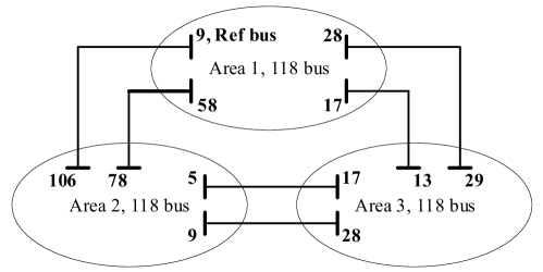
Figure 1: The three-area network for multi-area optimal power flow simulations, obtained by joining three IEEE 118-bus systems.
Refer to caption
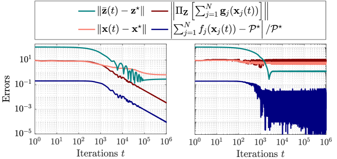
Figure 2: Performance of Algorithm 1 (left) and Algorithm 2 (right) on 𝒫1subscript𝒫1{\cal P}_{1} for the network in Figure 3.
Refer to caption
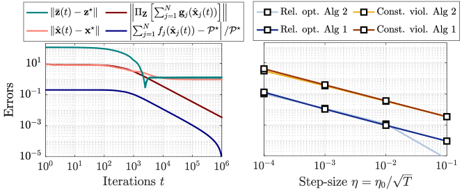
Figure 3: Performance of Algorithm 2 with primal averaging (left) and the impact of step-size on Algorithms 1 and 2 with primal averaging (right).

Consider the three-area power system shown in Figure 3 that comprises three IEEE 118 systems stitched together with 6 tie-lines as shown. The three systems were modified as delineated in [6, Appendix B1]. We applied Algorithm 1 on a reformulation of 𝒫1subscript𝒫1{\cal P}_{1} as an instance of 𝒫𝒫{\cal P} with a flat start (𝒛j(1)=0subscript𝒛𝑗10{\bm{z}}_{j}(1)=0, 𝒁j(0)=0subscript𝒁𝑗00{\bm{Z}}_{j}(0)=0, j=1,,N𝑗1𝑁j=1,\ldots,N) and step size η=η0/T𝜂subscript𝜂0𝑇\eta=\eta_{0}/\sqrt{T}, where η0=102subscript𝜂0superscript102\eta_{0}=10^{2} and T=106𝑇superscript106T=10^{6}. The results are portrayed on the left of Figure 3. We chose 𝑾𝑾{\bm{W}} based on the transition probabilities of a Markov chain in the Metropolis-Hastings algorithm (see [31, Sec. 2.5]). Here, 𝒫superscript𝒫{\cal P}^{\star} was computed by solving 𝒫1subscript𝒫1{\cal P}_{1} as a linear program. Our simulations were performed in MATLAB 2018b. All sub-problems were solved via MOSEK version 9.2.17.

1
2Choose 𝒛j(1)=0subscript𝒛𝑗10{\bm{z}}_{j}(1)=0 and η=η0/T𝜂subscript𝜂0𝑇\eta=\eta_{0}/\sqrt{T}.
3for t=1,,T𝑡1𝑇t=1,\ldots,T do
4      
5      𝒙j(t)argmin𝒙j𝕏jj(𝒙j,𝒛j(t))subscript𝒙𝑗𝑡subscriptargminsubscript𝒙𝑗subscript𝕏𝑗subscript𝑗subscript𝒙𝑗subscript𝒛𝑗𝑡{\bm{x}}_{j}(t)\leftarrow\mathop{\rm argmin}_{{\bm{x}}_{j}\in\mathds{X}_{j}}\ {\cal L}_{j}({\bm{x}}_{j},{\bm{z}}_{j}(t)).
6      𝒛j(t+1)k=1NWjkπ[𝒛k(t)+η𝒈k(𝒙k(t))]subscript𝒛𝑗𝑡1superscriptsubscript𝑘1𝑁subscript𝑊𝑗𝑘subscriptπdelimited-[]subscript𝒛𝑘𝑡𝜂subscript𝒈𝑘subscript𝒙𝑘𝑡{\bm{z}}_{j}({t+1})\leftarrow\sum_{k=1}^{N}W_{jk}{\uppi}_{\mathds{Z}}\left[{\bm{z}}_{k}(t)+\eta{\bm{g}}_{k}({\bm{x}}_{k}(t))\right].
7 end for
8
Algorithm 2 Distributed dual subgradient to solve 𝒫𝒫{\cal P}.

We compared Algorithm 1 with the classical dual subgradient method in Algorithm 2 (the projection and the consensus operations in step 2 are sometimes reversed, e.g., in [34]). The progress of Algorithm 2 with the same step-size used for Algorithm 1 are shown in the right of Figure 3. Note that Algorithm 1 leads to much smoother progress of j=1Nfj(𝒙j(t))superscriptsubscript𝑗1𝑁subscript𝑓𝑗subscript𝒙𝑗𝑡\sum_{j=1}^{N}f_{j}({\bm{x}}_{j}(t)) compared to that with Algorithm 2. Classical dual subgradient with primal averaging via 𝒙^j(t):=1tr=1t𝒙j(r)assignsubscript^𝒙𝑗𝑡1𝑡superscriptsubscript𝑟1𝑡subscript𝒙𝑗𝑟\hat{{\bm{x}}}_{j}(t):=\frac{1}{t}\sum_{r=1}^{t}{\bm{x}}_{j}(r) for each j=1,,N𝑗1𝑁j=1,\ldots,N can prevent this “flutter” (see [28, Section 4]), as the left plot in Figure 3 reveals. While step 1 of Algorithm 1 executes a similar averaging operation, this averaging step cannot be viewed as an output of the iteration dynamics as is the case for Algorithm 2 with averaging. As a result, the last iterate of Algorithm 1 moves smoothly as opposed to Algorithm 2. Such an update is useful in applications that require iterates to be directly implemented as control actions and the dual subgradient is only available at the current iterate (see [30] for a detailed discussion).

In the right of Figure 3, we compared the impact of step-size on the performance of Algorithms 1 and 2 with primal averaging after T=106𝑇superscript106T=10^{6} iterations. Here, relative optimality measures |j=1Nfj(𝒙j(t))𝒫|/𝒫superscriptsubscript𝑗1𝑁subscript𝑓𝑗subscript𝒙𝑗𝑡superscript𝒫superscript𝒫\left|\sum_{j=1}^{N}f_{j}({\bm{x}}_{j}(t))-{\cal P}^{\star}\right|/{\cal P}^{\star} and constraint violation measures π[i=1N𝒈j(𝒙j(T))]normsubscriptπdelimited-[]superscriptsubscript𝑖1𝑁subscript𝒈𝑗subscript𝒙𝑗𝑇\left\|{\uppi}_{\mathds{Z}}[\sum_{i=1}^{N}{\bm{g}}_{j}({\bm{x}}_{j}(T))]\right\| for Algorithm 1 and the same at 𝒙^j(t)subscript^𝒙𝑗𝑡\hat{{\bm{x}}}_{j}(t)’s for Algorithm 2. Empirically, constraint violation for Algorithm 1 appears similar to that for Algorithm 2 with primal averaging that is known to have 𝒪(T1/2)𝒪superscript𝑇12{\cal O}(T^{-1/2}) decay rate, much better than that suggested by (18) for Algorithm 1.

5 Grid Optimization Example 2: DER Coordination

Our next application problem is the coordination of DERs such as thermostatically controlled loads, electric vehicles, distributed rooftop solar, etc. that are increasingly getting adopted in distribution grids. There is a long literature on DER coordination to fulfill a variety of objectives that range from tracking a regulation signal at the T&D interface, to volt/VAR control within the distribution grid, etc. (e.g., see [36, 10]) See [6] for a longer list.

We formulate the DER coordination problem 𝒫2subscript𝒫2{\cal P}_{2} over a balanced three-phase radial distribution network on N𝑁N buses, described by graph 𝔊(N,𝔼)𝔊𝑁𝔼{\mathfrak{G}}(N,\mathds{E}). Let the first bus be the T&D interface. Associate directions to edges in 𝔼𝔼\mathds{E} arbitrarily to obtain a directed graph 𝔊(N,𝔼)𝔊𝑁𝔼\vec{{\mathfrak{G}}}(N,\vec{\mathds{E}}), where jk𝔼𝑗𝑘𝔼j\to k\in\vec{\mathds{E}} denotes a directed edge from bus j𝑗j to bus k𝑘k in 𝔊𝔊\vec{{\mathfrak{G}}}. At each bus j𝑗j, consider a dispatchable asset capable of injecting real and reactive powers pjG,qjGsubscriptsuperscript𝑝𝐺𝑗subscriptsuperscript𝑞𝐺𝑗p^{G}_{j},q^{G}_{j}, respectively. Let cj(pjG,qjG)subscript𝑐𝑗subscriptsuperscript𝑝𝐺𝑗subscriptsuperscript𝑞𝐺𝑗c_{j}(p^{G}_{j},q^{G}_{j}) denote the cost of power procurement from that dispatchable asset. At j=1𝑗1j=1, this cost might reflect the cost of procuring power from the transmission grid. It can also encode deviation of the power injection from a set point defined by a frequency regulation signal. At buses j=2,,N𝑗2𝑁j=2,\ldots,N, the cost can encode the disutility of deferred demand or cost of power production from dispatchable generation. The power injection capabilities of this asset at bus j𝑗j are limited as p¯jGpjGp¯jGsuperscriptsubscript¯𝑝𝑗𝐺superscriptsubscript𝑝𝑗𝐺superscriptsubscript¯𝑝𝑗𝐺\underline{p}_{j}^{G}\leq p_{j}^{G}\leq\overline{p}_{j}^{G} along with

q¯jGqjGq¯jG or [pjG]2+[pjG]2[s¯jG]2,superscriptsubscript¯𝑞𝑗𝐺superscriptsubscript𝑞𝑗𝐺superscriptsubscript¯𝑞𝑗𝐺 or superscriptdelimited-[]superscriptsubscript𝑝𝑗𝐺2superscriptdelimited-[]superscriptsubscript𝑝𝑗𝐺2superscriptdelimited-[]superscriptsubscript¯𝑠𝑗𝐺2\displaystyle\underline{q}_{j}^{G}\leq q_{j}^{G}\leq\overline{q}_{j}^{G}\text{ or }\left[p_{j}^{G}\right]^{2}+\left[p_{j}^{G}\right]^{2}\leq\left[\overline{s}_{j}^{G}\right]^{2},

henceforth denoted as (pjG,qjG)𝕊jsuperscriptsubscript𝑝𝑗𝐺superscriptsubscript𝑞𝑗𝐺subscript𝕊𝑗(p_{j}^{G},q_{j}^{G})\in\mathds{S}_{j}. Such models encompass photovoltaic and energy storage systems, water pumps, commercial HVAC systems, etc. At each bus j𝑗j, also assume nominal real and reactive power demands pjDsubscriptsuperscript𝑝𝐷𝑗p^{D}_{j} and qjDsubscriptsuperscript𝑞𝐷𝑗q^{D}_{j}.

We need additional notation to describe the DER coordination problem. Associate with bus j𝑗j the squared voltage magnitude wjsubscript𝑤𝑗w_{j}, deemed to lie in [w¯j,w¯j]subscript¯𝑤𝑗subscript¯𝑤𝑗[\underline{w}_{j},\overline{w}_{j}]. Let Pj,ksubscript𝑃𝑗𝑘P_{j,k}, Qj,ksubscript𝑄𝑗𝑘Q_{j,k} denote the real and reactive power flows from bus j𝑗j to bus k𝑘k for jk𝑗𝑘j\to k in 𝔊𝔊\vec{{\mathfrak{G}}}. Denote by j,ksubscript𝑗𝑘\ell_{j,k}, the squared current magnitude flowing from bus j𝑗j to bus k𝑘k, upper bounded by Lj,ksubscript𝐿𝑗𝑘L_{j,k}. Let 𝓇𝒿,𝓀subscript𝓇𝒿𝓀\mathpzc{r}_{j,k} and 𝓍𝒿,𝓀subscript𝓍𝒿𝓀\mathpzc{x}_{j,k} denote the resistance and reactance of the line jk𝑗𝑘j\to k. The DER coordination problem with a second-order conic relaxation of power flow equations in the radial distribution network can be formulated as

𝒫2::subscript𝒫2absent\displaystyle{\cal P}_{2}:\ minimizej=1Ncj(pjG,qjG),minimizesuperscriptsubscript𝑗1𝑁subscript𝑐𝑗subscriptsuperscript𝑝𝐺𝑗subscriptsuperscript𝑞𝐺𝑗\displaystyle\text{minimize}\quad\sum_{j=1}^{N}c_{j}(p^{G}_{j},q^{G}_{j}),
subject to
(pjG,qjG)𝕊j,superscriptsubscript𝑝𝑗𝐺superscriptsubscript𝑞𝑗𝐺subscript𝕊𝑗\displaystyle\qquad\left(p_{j}^{G},q_{j}^{G}\right)\in\mathds{S}_{j}, (54a)
pjGpjD=k:jkPj,kk:kj(Pk,j𝓇𝓀,𝒿𝓀,𝒿),superscriptsubscript𝑝𝑗𝐺superscriptsubscript𝑝𝑗𝐷subscript:𝑘𝑗𝑘subscript𝑃𝑗𝑘subscript:𝑘𝑘𝑗subscript𝑃𝑘𝑗subscript𝓇𝓀𝒿subscript𝓀𝒿\displaystyle\qquad p_{j}^{G}-p_{j}^{D}=\sum_{k:j\to k}{P_{j,k}}-\sum_{k:k\to j}{(P_{k,j}-\mathpzc{r}_{k,j}\ell_{k,j})}, (54b)
qjGqjD=k:jkQj,kk:kj(Qj,k𝓍𝓀,𝒿𝓀,𝒿),superscriptsubscript𝑞𝑗𝐺superscriptsubscript𝑞𝑗𝐷subscript:𝑘𝑗𝑘subscript𝑄𝑗𝑘subscript:𝑘𝑘𝑗subscript𝑄𝑗𝑘subscript𝓍𝓀𝒿subscript𝓀𝒿\displaystyle\qquad q_{j}^{G}-q_{j}^{D}=\sum_{k:j\to k}{Q_{j,k}}-\sum_{k:k\to j}{(Q_{j,k}-\mathpzc{x}_{k,j}\ell_{k,j})}, (54c)
wk=wj2(𝓇𝒿,𝓀𝒫𝒿,𝓀+𝓍𝒿,𝓀𝒬𝒿,𝓀)+(𝓇𝒿,𝓀2+𝓍𝒿,𝓀2)𝒿,𝓀,subscript𝑤𝑘subscript𝑤𝑗2subscript𝓇𝒿𝓀subscript𝒫𝒿𝓀subscript𝓍𝒿𝓀subscript𝒬𝒿𝓀superscriptsubscript𝓇𝒿𝓀2superscriptsubscript𝓍𝒿𝓀2subscript𝒿𝓀\displaystyle\qquad w_{k}=w_{j}-2(\mathpzc{r}_{j,k}P_{j,k}+\mathpzc{x}_{j,k}Q_{j,k})+(\mathpzc{r}_{j,k}^{2}+\mathpzc{x}_{j,k}^{2})\ell_{j,k}, (54d)
j,kLj,k,w¯jwjw¯j,formulae-sequencesubscript𝑗𝑘subscript𝐿𝑗𝑘subscript¯𝑤𝑗subscript𝑤𝑗subscript¯𝑤𝑗\displaystyle\qquad\ell_{j,k}\leq L_{j,k},\ \underline{w}_{j}\leq w_{j}\leq\overline{w}_{j}, (54e)
j,kwjPj,k2+Qj,k2,subscript𝑗𝑘subscript𝑤𝑗superscriptsubscript𝑃𝑗𝑘2superscriptsubscript𝑄𝑗𝑘2\displaystyle\qquad\ell_{j,k}w_{j}\geq P_{j,k}^{2}+Q_{j,k}^{2}, (54f)
j=1,,N,jk𝔊.formulae-sequence𝑗1𝑁𝑗𝑘𝔊\displaystyle\qquad j=1,\ldots,N,j\to k\in\ \vec{{\mathfrak{G}}}.

The last inequality is a second-order cone constraint, making (54) a second-order cone program (SOCP). Constraints in (54b), (54c) describe real and reactive power balance at each bus. Relations (54b), (54c), (54c), and the inequality in (54f) replaced with an equality define the feasible set described by AC power flow equations (see [13, 23] for details).

To cast 𝒫3subscript𝒫3{\cal P}_{3} as an instance of 𝒫𝒫{\cal P}, we first write the out-neighbors of j𝑗j in 𝔊𝔊\vec{{\mathfrak{G}}} as k1,,kJsubscript𝑘1subscript𝑘𝐽k_{1},\ldots,k_{J} and identify

𝒙j:=(pjG,qjG,wj,Pj,k1,,Pj,kJ,Qj,k1,,Qj,kJ,j,k1,,j,kJ),assignsubscript𝒙𝑗superscriptsuperscriptsubscript𝑝𝑗𝐺superscriptsubscript𝑞𝑗𝐺subscript𝑤𝑗subscript𝑃𝑗subscript𝑘1subscript𝑃𝑗subscript𝑘𝐽subscript𝑄𝑗subscript𝑘1subscript𝑄𝑗subscript𝑘𝐽subscript𝑗subscript𝑘1subscript𝑗subscript𝑘𝐽\displaystyle{\bm{x}}_{j}:=\left(p_{j}^{G},q_{j}^{G},w_{j},P_{j,k_{1}},\ldots,P_{j,k_{J}},Q_{j,k_{1}},\ldots,Q_{j,k_{J}},\ell_{j,k_{1}},\ldots,\ell_{j,k_{J}}\right)^{\mathchoice{\raisebox{0.75346pt}{$\displaystyle\intercal$}}{\raisebox{0.75346pt}{$\textstyle\intercal$}}{\raisebox{0.75346pt}{$\scriptstyle\intercal$}}{\raisebox{0.75346pt}{$\scriptscriptstyle\intercal$}}},
𝕏j:={𝒙j|(54a),(54e),(54f)},fj(𝒙j)=cj(pjG,qjG).formulae-sequenceassignsubscript𝕏𝑗conditional-setsubscript𝒙𝑗italic-(54aitalic-)italic-(54eitalic-)italic-(54fitalic-)subscript𝑓𝑗subscript𝒙𝑗subscript𝑐𝑗superscriptsubscript𝑝𝑗𝐺superscriptsubscript𝑞𝑗𝐺\displaystyle\mathds{X}_{j}:=\{{\bm{x}}_{j}\ |\ \eqref{eq:DER.1},\eqref{eq:DER.5},\eqref{eq:DER.6}\},\ f_{j}({\bm{x}}_{j})=c_{j}(p_{j}^{G},q_{j}^{G}).

Then, it is straightforward to write (54b), (54c) and (54d) as examples of (1b). This formulation does not require inequality constraints of the form (1c). Note T&D interface’s energy balancing and voltage constraints (54b)-(54d) can be treated as (1d) since there is no coupling variable from adjacent agents.

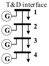
We ran Algorithm 1 on 𝒫2subscript𝒫2{\cal P}_{2} over a modified IEEE 4-bus radial distribution network (see [6, Appendix B2] for details).
Refer to caption
(a)
Refer to caption
(b)
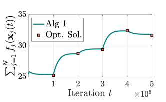
Figure 4: (a) A 4-bus radial network. (b) Progress of the objective function at the last iterate of Algorithm 1 on 𝒫2subscript𝒫2{\cal P}_{2} for the network in Figure 4a.

System conditions in the distribution grid can change quite fast. One line of work on DER coordination solves optimization problems in quick successions to deal with such changes, e.g., in [38]. To illustrate the use of DER coordination with time-varying distribution grid conditions, we simulated a case where real and reactive power demands were changed every 106superscript10610^{6} iterations as prescribed in [6, Appendix B2] with step-size η=0.1𝜂0.1\eta=0.1. Algorithm 1 is restarted after every change. Here, we use the last primal-dual iterate at the point of change to restart Algorithm 1. As Figure 4b illustrates, Algorithm 1 can track the optimal cost in the changing problem environment.
Refer to caption
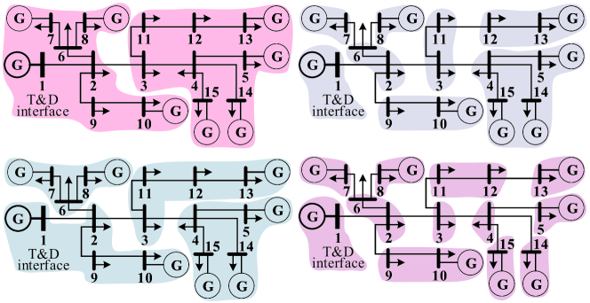
Figure 5: The IEEE 15-bus test feeder subdivided into 2, 4, 8 and 12 groups.
Refer to caption
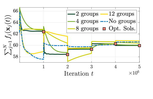
Figure 6: Evolution of the objective function value of Algorithm 1 on the IEEE 15-bus test system with varying degrees of decentralization (based on groupings of buses per Figure 6).

Convergence slows down over larger networks. Consider a modified IEEE 15-bus radial distribution network; see [6, Appendix B2] for the modifications. Figure 6 illustrates that Algorithm 1 with restarts is able to track optimal costs, but only when nodes are grouped together into fewer agents in 𝒫𝒫{\cal P}, as shown in Figure 6. Such a slowdown is expected, given that the convergence guarantees depend on N𝑁N, albeit polynomially. We remark that all first-order algorithms suffer from this issue. In practical implementation, one must carefully explore the trade-off between the degree of decentralization and the accuracy of tracking within a fixed number of iterations.

6 Grid Optimization Example 3: T&D Coordination

The lack of visibility of transmission SOs into distribution grids and bottlenecks in wholesale market clearing software make it impossible for such SOs to directly harness the flexibility offered by DERs in the distribution networks. Naturally, distributed algorithms are suited for T&D coordination; see [6] for prior art. Assume that for each distribution network, an aggregator 𝒜𝒜{\cal A} directly controls the dispatchable DERs and knows the network parameters. In what follows, we present the T&D coordination problem 𝒫3subscript𝒫3{\cal P}_{3} that a transmission SO and a collection of distribution aggregators solve in a distributed fashion. We utilize a semidefinite relaxation of power flow equations for the transmission network and a linear distribution flow model for the distribution grids.

To formulate the joint dispatch problem of all T&D assets, we require three different graphs. The first among these is the transmission network, modeled as an undirected graph 𝔊transuperscript𝔊tran{\mathfrak{G}}^{\textrm{tran}} on ntransuperscript𝑛trann^{\textrm{tran}} transmission buses. The second set of graphs are the distribution grids that connect to the transmission network at their points of common coupling–the ntransuperscript𝑛trann^{\textrm{tran}} transmission buses. We model the distribution grid connected to transmission bus \ell as an undirected graph 𝔊distsubscriptsuperscript𝔊dist{\mathfrak{G}}^{\textrm{dist}}_{\ell} on ndist+1subscriptsuperscript𝑛dist1n^{\textrm{dist}}_{\ell}+1 distribution buses, where the first bus of 𝔊distsubscriptsuperscript𝔊dist{\mathfrak{G}}^{\textrm{dist}}_{\ell} coincides with bus \ell in 𝔊transuperscript𝔊tran{\mathfrak{G}}^{\textrm{tran}}. Finally, we consider an undirected star graph 𝔊𝔊{\mathfrak{G}} on N=ntran+1𝑁superscript𝑛tran1N=n^{\textrm{tran}}+1 nodes with the aggregators 𝒜1,,𝒜ntransubscript𝒜1subscript𝒜superscript𝑛tran{\cal A}_{1},\ldots,{\cal A}_{n^{\textrm{tran}}} as the satellite nodes and the SO (the N𝑁N-th node) at the center.

Let 𝑽n𝑽superscript𝑛{\bm{V}}\in\mathds{C}^{n} denote the vector of nodal voltage phasors, where \mathds{C} is the set of complex numbers. We formulate the engineering constraints of the grid using the positive semidefinite matrix 𝚲:=𝑽𝑽𝖧ntran×ntranassign𝚲𝑽superscript𝑽𝖧superscriptsuperscript𝑛transuperscript𝑛tran{\bm{\Lambda}}:={\bm{V}}{\bm{V}}^{\sf{H}}\in\mathds{C}^{n^{\textrm{tran}}\times n^{\textrm{tran}}}. To describe these constraints, let y,k=yk,subscript𝑦𝑘subscript𝑦𝑘y_{\ell,k}=y_{k,\ell} denote the admittance of the transmission line joining buses ,k𝑘\ell,k in 𝔊transuperscript𝔊tran{\mathfrak{G}}^{\textrm{tran}} and y,subscript𝑦y_{\ell,\ell} denote the shunt admittance at bus \ell. Then, define 𝚽,ksubscript𝚽𝑘{\bm{\Phi}}_{\ell,k}, 𝚿,ksubscript𝚿𝑘{\bm{\Psi}}_{\ell,k} as the ntran×ntransuperscript𝑛transuperscript𝑛trann^{\textrm{tran}}\times n^{\textrm{tran}} Hermitian matrices whose only nonzero entries are

[𝚽,k],:=12(y,k+y,k𝖧),[𝚽,k],k=[𝚽,k]k,𝖧:=12y,k,formulae-sequenceassignsubscriptdelimited-[]subscript𝚽𝑘12subscript𝑦𝑘superscriptsubscript𝑦𝑘𝖧subscriptdelimited-[]subscript𝚽𝑘𝑘superscriptsubscriptdelimited-[]subscript𝚽𝑘𝑘𝖧assign12subscript𝑦𝑘\displaystyle[{\bm{\Phi}}_{\ell,k}]_{\ell,\ell}:=\frac{1}{2}(y_{\ell,k}+y_{\ell,k}^{\sf{H}}),[{\bm{\Phi}}_{\ell,k}]_{\ell,k}=[{\bm{\Phi}}_{\ell,k}]_{k,\ell}^{\sf{H}}:=-\frac{1}{2}y_{\ell,k},
[𝚿,k],:=12𝒊(y,k𝖧y,k),[𝚿,k],k=[𝚿,k]k,𝖧:=12𝒊y,k.formulae-sequenceassignsubscriptdelimited-[]subscript𝚿𝑘12𝒊superscriptsubscript𝑦𝑘𝖧subscript𝑦𝑘subscriptdelimited-[]subscript𝚿𝑘𝑘superscriptsubscriptdelimited-[]subscript𝚿𝑘𝑘𝖧assign12𝒊subscript𝑦𝑘\displaystyle[{\bm{\Psi}}_{\ell,k}]_{\ell,\ell}:=\frac{1}{2{\bm{i}}}(y_{\ell,k}^{\sf{H}}-y_{\ell,k}),[{\bm{\Psi}}_{\ell,k}]_{\ell,k}=[{\bm{\Psi}}_{\ell,k}]_{k,\ell}^{\sf{H}}:=\frac{1}{2{\bm{i}}}y_{\ell,k}.

In addition, we define the ntran×ntransuperscript𝑛transuperscript𝑛tran{n^{\textrm{tran}}\times n^{\textrm{tran}}} Hermitian matrices

𝚽:=12(y,+y,𝖧)𝟙𝟙𝖧+k𝚽,k,𝚿:=12𝒊(y,𝖧y,)𝟙𝟙𝖧+k𝚿,k,\displaystyle{\bm{\Phi}}_{\ell}:=\frac{1}{2}\left({y_{\ell,\ell}+y_{\ell,\ell}^{\sf{H}}}\right){\mathds{1}}_{\ell}{\mathds{1}}_{\ell}^{\sf{H}}+\sum_{k\sim\ell}{\bm{\Phi}}_{\ell,k},\quad{\bm{\Psi}}_{\ell}:=\frac{1}{2{\bm{i}}}\left({y_{\ell,\ell}^{\sf{H}}-y_{\ell,\ell}}\right){\mathds{1}}_{\ell}{\mathds{1}}_{\ell}^{\sf{H}}+\sum_{k\sim\ell}{\bm{\Psi}}_{\ell,k},

where 𝟙1{\mathds{1}} is a vector of all ones of appropriate size and 𝟙subscript1{\mathds{1}}_{\ell} is a vector of all zeros except at the \ell-th position that is unity. This notation allows us to describe the apparent power flow from bus \ell to bus k𝑘k as Tr(𝚽,k𝚲)+𝒊Tr(𝚿,k𝚲)Trsubscript𝚽𝑘𝚲𝒊Trsubscript𝚿𝑘𝚲\mbox{\rm Tr}({\bm{\Phi}}_{\ell,k}{\bm{\Lambda}})+{\bm{i}}\mbox{\rm Tr}({\bm{\Psi}}_{\ell,k}{\bm{\Lambda}}), the apparent power injection at bus \ell as Tr(𝚽𝚲)+𝒊Tr(𝚿𝚲)Trsubscript𝚽𝚲𝒊Trsubscript𝚿𝚲\mbox{\rm Tr}({\bm{\Phi}}_{\ell}{\bm{\Lambda}})+{\bm{i}}\mbox{\rm Tr}({\bm{\Psi}}_{\ell}{\bm{\Lambda}}), and the squared voltage magnitude at bus \ell as Tr(𝟙𝟙𝖧𝚲)Trsubscript1superscriptsubscript1𝖧𝚲\mbox{\rm Tr}({\mathds{1}}_{\ell}{\mathds{1}}_{\ell}^{\sf{H}}{\bm{\Lambda}}), where 𝒊:=1assign𝒊1{\bm{i}}:=\sqrt{-1}. At each transmission bus \ell with load PD+𝒊QDsuperscriptsubscript𝑃𝐷𝒊superscriptsubscript𝑄𝐷P_{\ell}^{D}+{\bm{i}}Q_{\ell}^{D}, let a generator supply apparent power PG+𝒊QGsuperscriptsubscript𝑃𝐺𝒊superscriptsubscript𝑄𝐺P_{\ell}^{G}+{\bm{i}}Q_{\ell}^{G} with procurement cost described by Csubscript𝐶C_{\ell}.

Let each transmission bus \ell be the first bus of an ndist+1superscript𝑛dist1n^{\textrm{dist}}+1-bus distribution network 𝔊distsubscriptsuperscript𝔊dist{\mathfrak{G}}^{\textrm{dist}}_{\ell}. Let 𝒑+𝒊𝒒ndistsubscript𝒑𝒊subscript𝒒superscriptsuperscript𝑛dist{\bm{p}}_{\ell}+{\bm{i}}{\bm{q}}_{\ell}\in\mathds{C}^{n^{\textrm{dist}}} denote the vector of net power injections across the distribution network, save the first bus. Further, let the power procurement cost be given by 𝒄subscript𝒄{\bm{c}}_{\ell} to inject 𝒑+𝒊𝒒ndistsubscript𝒑𝒊subscript𝒒superscriptsuperscript𝑛dist{\bm{p}}_{\ell}+{\bm{i}}{\bm{q}}_{\ell}\in\mathds{C}^{n^{\textrm{dist}}}. Also, let 𝚲ndistsubscript𝚲superscriptsuperscript𝑛dist{\bm{\Lambda}}_{\ell}\in\mathds{C}^{n^{\textrm{dist}}} denote the vector of squared voltage magnitudes across the same set of buses. We adopt the popular LinDistFlow model to tackle the nonconvex nature of the power flow equations in the distribution grid. Let 𝑴~ndist×ndist~𝑴superscriptsuperscript𝑛distsuperscript𝑛dist\widetilde{{\bm{M}}}\in\mathds{R}^{n^{\textrm{dist}}\times n^{\textrm{dist}}} be the node-to-edge incidence matrix of 𝔊distsubscriptsuperscript𝔊dist{\mathfrak{G}}^{\textrm{dist}}_{\ell}. Further, remove the first row of 𝑴~~𝑴\widetilde{{\bm{M}}} to obtain the reduced incidence matrix 𝑴𝑴{\bm{M}}. Then, the voltage magnitudes are related to power injections under the LinDistFlow model as 𝚲=𝝆𝒑+𝝌𝒒+Λ,𝟙subscript𝚲subscript𝝆subscript𝒑subscript𝝌subscript𝒒subscriptΛ1{\bm{\Lambda}}_{\ell}={\bm{\rho}}_{\ell}{\bm{p}}_{\ell}+{\bm{\chi}}_{\ell}{\bm{q}}_{\ell}+\Lambda_{\ell,\ell}{\mathds{1}}, where 𝝆subscript𝝆{\bm{\rho}}_{\ell} and 𝝌subscript𝝌{\bm{\chi}}_{\ell} are ndist×ndistsuperscript𝑛distsuperscript𝑛distn^{\textrm{dist}}\times n^{\textrm{dist}} matrices defined as 𝝆:=2𝑴diag(r)𝑴1assignsubscript𝝆2superscript𝑴diagsubscriptrsuperscript𝑴1{\bm{\rho}}_{\ell}:=2{\bm{M}}^{-{\mathchoice{\raisebox{0.75346pt}{$\displaystyle\intercal$}}{\raisebox{0.75346pt}{$\textstyle\intercal$}}{\raisebox{0.75346pt}{$\scriptstyle\intercal$}}{\raisebox{0.75346pt}{$\scriptscriptstyle\intercal$}}}}\mathop{\mathrm{diag}}({{\bm{\mathpzc{r}}}_{\ell}}){\bm{M}}^{-1}, 𝝌:=2𝑴diag(x)𝑴1assignsubscript𝝌2superscript𝑴diagsubscriptxsuperscript𝑴1{\bm{\chi}}_{\ell}:=2{\bm{M}}^{-{\mathchoice{\raisebox{0.75346pt}{$\displaystyle\intercal$}}{\raisebox{0.75346pt}{$\textstyle\intercal$}}{\raisebox{0.75346pt}{$\scriptstyle\intercal$}}{\raisebox{0.75346pt}{$\scriptscriptstyle\intercal$}}}}\mathop{\mathrm{diag}}({{\bm{\mathpzc{x}}}_{\ell}}){\bm{M}}^{-1}, rsubscriptr{\bm{\mathpzc{r}}}_{\ell}/ xsubscriptx{\bm{\mathpzc{x}}}_{\ell} collect the resistances/reactances of the ndistsuperscript𝑛distn^{\textrm{dist}} distribution lines.

The optimal joint dispatch over all T&D assets is given by

𝒫3::subscript𝒫3absent\displaystyle{\cal P}_{3}:\ minimize =1ntranC(PG,QG)+=1ntran𝒄(𝒑G,𝒒G),superscriptsubscript1superscript𝑛transubscript𝐶subscriptsuperscript𝑃𝐺subscriptsuperscript𝑄𝐺superscriptsubscript1superscript𝑛transubscript𝒄subscriptsuperscript𝒑𝐺subscriptsuperscript𝒒𝐺\displaystyle\quad\sum_{\ell=1}^{n^{\textrm{tran}}}C_{\ell}(P^{G}_{\ell},Q^{G}_{\ell})+\sum_{\ell=1}^{n^{\textrm{tran}}}{\bm{c}}_{\ell}({\bm{p}}^{G}_{\ell},{\bm{q}}^{G}_{\ell}),
subject to (PG,QG)𝕊tran,superscriptsubscript𝑃𝐺superscriptsubscript𝑄𝐺subscriptsuperscript𝕊tran\displaystyle\quad({P}_{\ell}^{G},Q_{\ell}^{G})\in\mathds{S}^{\textrm{tran}}_{\ell}, (55a)
(𝒑G,𝒒G)𝕊dist,superscriptsubscript𝒑𝐺superscriptsubscript𝒒𝐺subscriptsuperscript𝕊dist\displaystyle\quad\left({\bm{p}}_{\ell}^{G},{\bm{q}}_{\ell}^{G}\right)\in\mathds{S}^{\textrm{dist}}_{\ell}, (55b)
PGPD+𝟙(𝒑G𝒑D)=Tr(𝚽𝚲),subscriptsuperscript𝑃𝐺superscriptsubscript𝑃𝐷superscript1subscriptsuperscript𝒑𝐺subscriptsuperscript𝒑𝐷Trsubscript𝚽𝚲\displaystyle\quad P^{G}_{\ell}-P_{\ell}^{D}+{\mathds{1}}^{\mathchoice{\raisebox{0.75346pt}{$\displaystyle\intercal$}}{\raisebox{0.75346pt}{$\textstyle\intercal$}}{\raisebox{0.75346pt}{$\scriptstyle\intercal$}}{\raisebox{0.75346pt}{$\scriptscriptstyle\intercal$}}}\left({\bm{p}}^{G}_{\ell}-{\bm{p}}^{D}_{\ell}\right)=\mbox{\rm Tr}({\bm{\Phi}}_{\ell}{\bm{\Lambda}}), (55c)
QGQD+𝟙(𝒒G𝒒D)=Tr(𝚿𝚲),subscriptsuperscript𝑄𝐺superscriptsubscript𝑄𝐷superscript1subscriptsuperscript𝒒𝐺subscriptsuperscript𝒒𝐷Trsubscript𝚿𝚲\displaystyle\quad Q^{G}_{\ell}-Q_{\ell}^{D}+{\mathds{1}}^{\mathchoice{\raisebox{0.75346pt}{$\displaystyle\intercal$}}{\raisebox{0.75346pt}{$\textstyle\intercal$}}{\raisebox{0.75346pt}{$\scriptstyle\intercal$}}{\raisebox{0.75346pt}{$\scriptscriptstyle\intercal$}}}\left({\bm{q}}^{G}_{\ell}-{\bm{q}}^{D}_{\ell}\right)=\mbox{\rm Tr}({\bm{\Psi}}_{\ell}{\bm{\Lambda}}), (55d)
Tr(𝚽,𝚲)L,,Trsubscript𝚽superscript𝚲subscript𝐿superscript\displaystyle\quad\mbox{\rm Tr}({\bm{\Phi}}_{\ell,\ell^{\prime}}{\bm{\Lambda}})\leq L_{\ell,\ell^{\prime}}, (55e)
w¯Λ,w¯,subscript¯𝑤subscriptΛsubscript¯𝑤\displaystyle\quad\underline{{w}}_{\ell}\leq\Lambda_{\ell,\ell}\leq\overline{{w}}_{\ell}, (55f)
𝚲0,succeeds-or-equals𝚲0\displaystyle\quad{\bm{\Lambda}}\succeq 0, (55g)
𝒘¯𝝆𝒑+𝝌𝒒+Λ,𝟙𝒘¯,subscript¯𝒘subscript𝝆subscript𝒑subscript𝝌subscript𝒒subscriptΛ1subscript¯𝒘\displaystyle\quad\underline{{{\bm{w}}}}_{\ell}\leq{\bm{\rho}}_{\ell}{\bm{p}}_{\ell}+{\bm{\chi}}_{\ell}{\bm{q}}_{\ell}+\Lambda_{\ell,\ell}{\mathds{1}}\leq\overline{{{\bm{w}}}}_{\ell}, (55h)
for =1,,ntran,.formulae-sequencefor 1superscript𝑛transimilar-tosuperscript\displaystyle\quad\text{for }\ell=1,\ldots,n^{\textrm{tran}},\ \ell^{\prime}\sim\ell.

Here, (55a), (55b) encode the capabilities of transmission and distribution assets, respectively, where 𝕊transuperscript𝕊tran\mathds{S}^{\textrm{tran}} and 𝕊distsuperscript𝕊dist\mathds{S}^{\textrm{dist}} are assumed convex. Constraints in (55c) and (55d) enforce nodal power balance at transmission nodes. Transmission line (real power) flows are constrained in (55e), with L𝐿L’s describing the line capacities. One can alternately constrain apparent power flows. Transmission voltage limits are enforced via (55f) within [w¯,w¯]subscript¯𝑤subscript¯𝑤[\underline{w}_{\ell},\overline{w}_{\ell}]. The relation 𝚲=𝑽𝑽𝖧𝚲𝑽superscript𝑽𝖧{\bm{\Lambda}}={\bm{V}}{\bm{V}}^{\sf{H}} requires 𝚲𝚲{\bm{\Lambda}} to be positive semidefinite (enforced in (55g)) and rank-1. We consider the rank-relaxed power flow equations by dropping the rank-1 requirement. For the distribution grid, voltage limits are enforced in (55h) and power flow limits are ignored.

Recall that 𝔊𝔊{\mathfrak{G}} for T&D coordination problem is a graph on N=ntran+1𝑁superscript𝑛tran1N=n^{\textrm{tran}}+1 nodes, where the first ntransuperscript𝑛trann^{\textrm{tran}} nodes are transmission buses and the last node represents the SO. Define

𝒙:=(𝒑,𝒒),𝕏:={𝒙|(55b)},f=c(𝒑G,𝒒G)formulae-sequenceassignsubscript𝒙superscriptsuperscriptsubscript𝒑superscriptsubscript𝒒formulae-sequenceassignsubscript𝕏conditional-setsubscript𝒙italic-(55bitalic-)subscript𝑓subscript𝑐subscriptsuperscript𝒑𝐺subscriptsuperscript𝒒𝐺\displaystyle{\bm{x}}_{\ell}:=\left({\bm{p}}_{\ell}^{\mathchoice{\raisebox{0.75346pt}{$\displaystyle\intercal$}}{\raisebox{0.75346pt}{$\textstyle\intercal$}}{\raisebox{0.75346pt}{$\scriptstyle\intercal$}}{\raisebox{0.75346pt}{$\scriptscriptstyle\intercal$}}},{\bm{q}}_{\ell}^{\mathchoice{\raisebox{0.75346pt}{$\displaystyle\intercal$}}{\raisebox{0.75346pt}{$\textstyle\intercal$}}{\raisebox{0.75346pt}{$\scriptstyle\intercal$}}{\raisebox{0.75346pt}{$\scriptscriptstyle\intercal$}}}\right)^{\mathchoice{\raisebox{0.75346pt}{$\displaystyle\intercal$}}{\raisebox{0.75346pt}{$\textstyle\intercal$}}{\raisebox{0.75346pt}{$\scriptstyle\intercal$}}{\raisebox{0.75346pt}{$\scriptscriptstyle\intercal$}}},\ \mathds{X}_{\ell}:=\{{\bm{x}}_{\ell}\ |\ \eqref{eq:TD.2}\},\ f_{\ell}=c_{\ell}({\bm{p}}^{G}_{\ell},{\bm{q}}^{G}_{\ell})

for =1,,ntran1superscript𝑛tran\ell=1,\ldots,n^{\textrm{tran}}. Collect the real and reactive power generations across the transmission grid in the vectors 𝑷G,𝑸Gsuperscript𝑷𝐺superscript𝑸𝐺{\bm{P}}^{G},{\bm{Q}}^{G}, respectively. Then, define

𝒙Nsubscript𝒙𝑁\displaystyle{\bm{x}}_{N} :=([𝑷G],[𝑸G],vec({𝚲}),vec({𝚲})),assignabsentsuperscriptsuperscriptdelimited-[]superscript𝑷𝐺superscriptdelimited-[]superscript𝑸𝐺vecsuperscript𝚲vecsuperscript𝚲\displaystyle:=\left([{\bm{P}}^{G}]^{\mathchoice{\raisebox{0.75346pt}{$\displaystyle\intercal$}}{\raisebox{0.75346pt}{$\textstyle\intercal$}}{\raisebox{0.75346pt}{$\scriptstyle\intercal$}}{\raisebox{0.75346pt}{$\scriptscriptstyle\intercal$}}},[{\bm{Q}}^{G}]^{\mathchoice{\raisebox{0.75346pt}{$\displaystyle\intercal$}}{\raisebox{0.75346pt}{$\textstyle\intercal$}}{\raisebox{0.75346pt}{$\scriptstyle\intercal$}}{\raisebox{0.75346pt}{$\scriptscriptstyle\intercal$}}},\textrm{vec}\left(\Re\{{\bm{\Lambda}}\}\right)^{\mathchoice{\raisebox{0.75346pt}{$\displaystyle\intercal$}}{\raisebox{0.75346pt}{$\textstyle\intercal$}}{\raisebox{0.75346pt}{$\scriptstyle\intercal$}}{\raisebox{0.75346pt}{$\scriptscriptstyle\intercal$}}},\textrm{vec}\left(\Im\{{\bm{\Lambda}}\}\right)^{\mathchoice{\raisebox{0.75346pt}{$\displaystyle\intercal$}}{\raisebox{0.75346pt}{$\textstyle\intercal$}}{\raisebox{0.75346pt}{$\scriptstyle\intercal$}}{\raisebox{0.75346pt}{$\scriptscriptstyle\intercal$}}}\right)^{\mathchoice{\raisebox{0.75346pt}{$\displaystyle\intercal$}}{\raisebox{0.75346pt}{$\textstyle\intercal$}}{\raisebox{0.75346pt}{$\scriptstyle\intercal$}}{\raisebox{0.75346pt}{$\scriptscriptstyle\intercal$}}},
𝕏Nsubscript𝕏𝑁\displaystyle\mathds{X}_{N} :={𝒙ntran+1|(55a),(55e),(55f),(55g)},assignabsentconditional-setsubscript𝒙superscript𝑛tran1italic-(55aitalic-)italic-(55eitalic-)italic-(55fitalic-)italic-(55gitalic-)\displaystyle:=\{{\bm{x}}_{n^{\textrm{tran}}+1}\ |\ \eqref{eq:TD.1},\eqref{eq:TD.5},\eqref{eq:TD.6},\eqref{eq:TD.7}\},
fN(𝒙N)subscript𝑓𝑁subscript𝒙𝑁\displaystyle f_{N}({\bm{x}}_{N}) ==1ntranC(PG,QG).absentsuperscriptsubscript1superscript𝑛transubscript𝐶superscriptsubscript𝑃𝐺superscriptsubscript𝑄𝐺\displaystyle=\sum_{\ell=1}^{n^{\textrm{tran}}}C_{\ell}(P_{\ell}^{G},Q_{\ell}^{G}).

The constraint (55g) can be written in terms of 𝒙Nsubscript𝒙𝑁{\bm{x}}_{N} as

({𝚲}{𝚲}{𝚲}{𝚲})0succeeds-or-equalsmatrix𝚲𝚲𝚲𝚲0\begin{pmatrix}\Re\{{\bm{\Lambda}}\}&\Im\{{\bm{\Lambda}}\}\\ -\Im\{{\bm{\Lambda}}\}&\Re\{{\bm{\Lambda}}\}\end{pmatrix}\succeq 0

and (55c) – (55d) as examples of (1b) using Tr(𝝋𝚲)=vec({𝝋})vec({𝚲})+vec({𝝋})vec({𝚲})Tr𝝋𝚲vecsuperscript𝝋vec𝚲vecsuperscript𝝋vec𝚲\mbox{\rm Tr}({\bm{\varphi}}{\bm{\Lambda}})=\textrm{vec}\left(\Re\{{\bm{\varphi}}\}\right)^{\mathchoice{\raisebox{0.75346pt}{$\displaystyle\intercal$}}{\raisebox{0.75346pt}{$\textstyle\intercal$}}{\raisebox{0.75346pt}{$\scriptstyle\intercal$}}{\raisebox{0.75346pt}{$\scriptscriptstyle\intercal$}}}\textrm{vec}\left(\Re\{{\bm{\Lambda}}\}\right)+\textrm{vec}\left(\Im\{{\bm{\varphi}}\}\right)^{\mathchoice{\raisebox{0.75346pt}{$\displaystyle\intercal$}}{\raisebox{0.75346pt}{$\textstyle\intercal$}}{\raisebox{0.75346pt}{$\scriptstyle\intercal$}}{\raisebox{0.75346pt}{$\scriptscriptstyle\intercal$}}}\textrm{vec}\left(\Im\{{\bm{\Lambda}}\}\right) for a Hermitian matrix 𝝋𝝋{\bm{\varphi}}. Constraints (55h) are examples of inequality constraints in (1c).
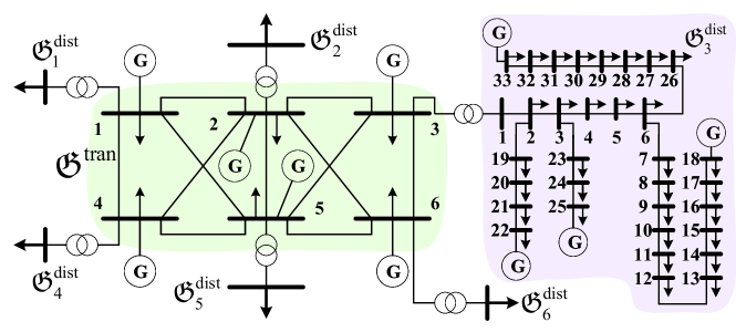
Refer to caption
Figure 7: The 204-bus network for T&D simulations, obtained by joining the IEEE 6-bus transmission network with six IEEE 33-bus distribution networks.
Refer to caption
Figure 8: Progress of Algorithm 1 on 𝒫3subscript𝒫3{\cal P}_{3}.

We report numerical results on a 204-bus T&D system that comprises the IEEE 6-bus transmission network joined with six IEEE 33-bus distribution systems (see Figure 8 and [6, Appendix B3] for details). We applied Algorithm 1 on a reformulation of 𝒫3subscript𝒫3{\cal P}_{3} as an instance of 𝒫𝒫{\cal P} with a flat start (𝒛j(1)=0subscript𝒛𝑗10{\bm{z}}_{j}(1)=0, 𝒁j(0)=0subscript𝒁𝑗00{\bm{Z}}_{j}(0)=0, j=1,,N𝑗1𝑁j=1,\ldots,N) and step size η=η0/T𝜂subscript𝜂0𝑇\eta=\eta_{0}/\sqrt{T}, where η0=103subscript𝜂0superscript103\eta_{0}=10^{3} and T=108𝑇superscript108T=10^{8}. The agent-wise subproblems for 𝒫3subscript𝒫3{\cal P}_{3} are communicated over a 7-node star graph 𝔊𝔊{\mathfrak{G}} with the SO in the center. Convergence results are shown in Figure 8.

One might surmise that dual subgradient methods can be accelerated à la Nesterov. Such acceleration requires smoothness of the dual function–a property that an application problem such as 𝒫3subscript𝒫3{\cal P}_{3} does not always possess. In Appendix A, we provide simple examples, where dual functions are nonsmooth, and show how the nonsmoothness impedes acceleration. We illustrate the same difficulty with 𝒫3subscript𝒫3{\cal P}_{3}. Specifically, we compare the performance of Algorithm 1 with a distributed acceleration scheme in [33, eq. (5)-(6)], adopted to our setup, described in Algorithm 3.

1
2Choose η=η0/T𝜂subscript𝜂0𝑇\eta=\eta_{0}/\sqrt{T}, 𝒛j(1)=𝒀j(1)=0subscript𝒛𝑗1subscript𝒀𝑗10{\bm{z}}_{j}(1)={\bm{Y}}_{j}(1)=0, α(1)=0.5𝛼10.5\alpha(1)=0.5, 𝒙j(1)argmin𝒙j𝕏jj(𝒙j,𝒛j(1))subscript𝒙𝑗1subscriptargminsubscript𝒙𝑗subscript𝕏𝑗subscript𝑗subscript𝒙𝑗subscript𝒛𝑗1{\bm{x}}_{j}(1)\leftarrow\mathop{\rm argmin}_{{\bm{x}}_{j}\in\mathds{X}_{j}}\ {\cal L}_{j}({\bm{x}}_{j},{\bm{z}}_{j}(1)), and 𝒔j(1)𝒈j(𝒙j(1))subscript𝒔𝑗1subscript𝒈𝑗subscript𝒙𝑗1{\bm{s}}_{j}(1)\leftarrow{\bm{g}}_{j}({\bm{x}}_{j}(1)).
3for t=1,,T𝑡1𝑇t=1,\ldots,T do
4      
5      𝒁j(t+1)k=1NWjk𝒛k(t)+η𝒔j(t)subscript𝒁𝑗𝑡1superscriptsubscript𝑘1𝑁subscript𝑊𝑗𝑘subscript𝒛𝑘𝑡𝜂subscript𝒔𝑗𝑡{\bm{Z}}_{j}(t+1)\leftarrow\sum_{k=1}^{N}W_{jk}{\bm{z}}_{k}(t)+\eta{\bm{s}}_{j}(t)
6      𝒀j(t+1)k=1NWjk𝒀k(t)+ηα(t)𝒔j(t)subscript𝒀𝑗𝑡1superscriptsubscript𝑘1𝑁subscript𝑊𝑗𝑘subscript𝒀𝑘𝑡𝜂𝛼𝑡subscript𝒔𝑗𝑡{\bm{Y}}_{j}(t+1)\leftarrow\sum_{k=1}^{N}W_{jk}{\bm{Y}}_{k}(t)+\frac{\eta}{\alpha(t)}{\bm{s}}_{j}(t)
7      α(t+1)12[α(t)2+α(t)4+4α(t)2]𝛼𝑡112delimited-[]𝛼superscript𝑡2𝛼superscript𝑡44𝛼superscript𝑡2\alpha(t+1)\leftarrow\frac{1}{2}\left[-\alpha(t)^{2}+\sqrt{\alpha(t)^{4}+4\alpha(t)^{2}}\right]
8      𝒛j(t+1)π[(1α(t+1))𝒁j(t+1){\bm{z}}_{j}({t+1})\leftarrow{\uppi}_{\mathds{Z}}\left[(1-\alpha(t+1)){\bm{Z}}_{j}(t+1)\right. +α(t+1)𝒀j(t+1)]\left.+\alpha(t+1){\bm{Y}}_{j}(t+1)\right]
9      𝒙j(t+1)argmin𝒙j𝕏jj(𝒙j,𝒛j(t+1))subscript𝒙𝑗𝑡1subscriptargminsubscript𝒙𝑗subscript𝕏𝑗subscript𝑗subscript𝒙𝑗subscript𝒛𝑗𝑡1{\bm{x}}_{j}(t+1)\leftarrow\mathop{\rm argmin}_{{\bm{x}}_{j}\in\mathds{X}_{j}}\ {\cal L}_{j}({\bm{x}}_{j},{\bm{z}}_{j}(t+1))
10      𝒔j(t+1)k=1NWjk𝒔k(t)+𝒈j(𝒙j(t+1))𝒈j(𝒙j(t))subscript𝒔𝑗𝑡1superscriptsubscript𝑘1𝑁subscript𝑊𝑗𝑘subscript𝒔𝑘𝑡subscript𝒈𝑗subscript𝒙𝑗𝑡1subscript𝒈𝑗subscript𝒙𝑗𝑡{\bm{s}}_{j}({t+1})\leftarrow\sum_{k=1}^{N}W_{jk}{\bm{s}}_{k}(t)+{\bm{g}}_{j}({\bm{x}}_{j}(t+1))-{\bm{g}}_{j}({\bm{x}}_{j}(t))
11 end for
Algorithm 3 Accelerated distributed dual subgradient to solve 𝒫𝒫{\cal P}.

In this algorithm, the dual ancillary sequences 𝒁j(t)subscript𝒁𝑗𝑡{\bm{Z}}_{j}(t), 𝒀j(t)subscript𝒀𝑗𝑡{\bm{Y}}_{j}(t) in steps 3-3 are averaged by α(t)𝛼𝑡\alpha(t) in step 3 that is updated in step 3. The distributed acceleration scheme in [33, eq. (5)-(6)] has been designed for unconstrained optimization problems; we project multipliers of constraints (55h) in step 3 on the positive orthant to apply it to 𝒫3subscript𝒫3{\cal P}_{3}. Each local problem is solved in step 3 to obtain the local dual subgradient 𝒈j(𝒙j(t+1))subscript𝒈𝑗subscript𝒙𝑗𝑡1{\bm{g}}_{j}({\bm{x}}_{j}(t+1)). The central subgradient is approximated in step 3 that combines consensus tracking and local gradient averaging.

The results are shown in Figure 9. Here, we adopted cold start for the dual iterates for both algorithms, i.e., 𝒛j(1)=𝟎,j=1,,Nformulae-sequencesubscript𝒛𝑗10𝑗1𝑁{\bm{z}}_{j}(1)={\bm{0}},\ j=1,\ldots,N. We show the case when generation costs for real power are considered quadratic on the left. The figure on the right is derived with linear real power generation costs. All reactive generation costs are considered quadratic for both simulations. Quadratic costs often yield a smooth dual function that Algorithm 3 can exploit and attain faster convergence than Algorithm 1. With linear costs, the dual function can be non-differentiable (especially at an optimal dual solution) as a result of primal non-uniqueness [2, Theorem 6.3.3]. Nonsmoothness is a fundamental barrier to acceleration as our example reveals. We discuss the role of smoothness of the dual function in acceleration further in Appendix A through illustrative examples.
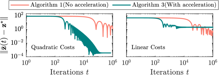
Refer to caption
Figure 9: Convergence of dual iterates on 𝒫3subscript𝒫3{\cal P}_{3} about Algorithm 1 (no acceleration) and Algorithm 3 from [33, eq. (5)-(6)] (with acceleration).

7 Concluding Remarks

We have studied a constant step-size distributed dual subgradient (DDSG) method with averaging that provides order-optimal 1/T1𝑇1/\sqrt{T} convergence rate after T𝑇T iterations for multi-agent convex constrained optimization problems of the form 𝒫𝒫{\cal P} whose objective function need not be strongly convex. The convergence guarantee improves the rate of the decaying step-size, fully decentralized counterpart studied in [22]. We formulated a variety of problems that arise in the operation of an electric power system as examples of 𝒫𝒫{\cal P} and applied the DDSG method to solve them. The case studies with DDSG on grid optimization problems are presented not to empirically challenge other methods in the literature, but as means to illustrate the broad applicability of optimization problems such as 𝒫𝒫{\cal P} to facilitate unified algorithm development. These examples also underscore various properties of the DDSG algorithm. Specifically, the first example illustrates the difference in performance of the last iterate between the vanilla DDSG method and ours. The second example reveals the effect of the number of agents on convergence speed. The third example empirically studies the possibility of Nesterov-style acceleration in DDSG methods and the role that smoothness in the dual function plays in such analysis.

Several research directions are of interest to us. The first among them is an algorithm with last-iterate guarantees over time-varying communication networks. The second important direction is to better disentangle the error 𝒱Tsubscript𝒱𝑇{\cal V}_{T} to provide guarantees on suboptimality and constraint violation separately. Third, we want to explore ways to exploit a similar algorithmic architecture for stochastic and risk-sensitive convex optimization problems.

Appendix

Appendix A Dual subgradient methods cannot generally be accelerated

Nesterov-type acceleration relies on smoothness of the objective function. Here, we illustrate why such acceleration is generally untenable in dual subgradient settings. We first present examples where the dual function for constrained optimization problems are nonsmooth. Then, we illustrate through examples how nonsmoothness of the objective function impairs acceleration. Consider an optimization problem of the form

minimize𝒙𝕏12𝒙𝚵𝒙+𝝃𝒙+ν,subject to𝑨𝒙𝒃.𝒙𝕏minimize12superscript𝒙𝚵𝒙superscript𝝃𝒙𝜈subject to𝑨𝒙𝒃\displaystyle\underset{{\bm{x}}\in\mathds{X}}{\text{minimize}}\ \frac{1}{2}{\bm{x}}^{\mathchoice{\raisebox{0.75346pt}{$\displaystyle\intercal$}}{\raisebox{0.75346pt}{$\textstyle\intercal$}}{\raisebox{0.75346pt}{$\scriptstyle\intercal$}}{\raisebox{0.75346pt}{$\scriptscriptstyle\intercal$}}}{\bm{\Xi}}{\bm{x}}+{\bm{\xi}}^{\mathchoice{\raisebox{0.75346pt}{$\displaystyle\intercal$}}{\raisebox{0.75346pt}{$\textstyle\intercal$}}{\raisebox{0.75346pt}{$\scriptstyle\intercal$}}{\raisebox{0.75346pt}{$\scriptscriptstyle\intercal$}}}{\bm{x}}+\nu,\ \ \text{subject to}\ {\bm{A}}{\bm{x}}\leq{\bm{b}}. (56)

with 𝚵𝚵{\bm{\Xi}} being positive semidefinite (but not positive definite) and 𝕏𝕏\mathds{X} being a convex polyhedral set. This is a quadratic program (QP) that simplifies to a linear program (LP) when 𝚵=0𝚵0{\bm{\Xi}}=0. Associate multipliers 𝒛0𝒛0{\bm{z}}\geq 0 with 𝑨𝒙𝒃𝑨𝒙𝒃{\bm{A}}{\bm{x}}\leq{\bm{b}}. Then, the dual function for the problem in (56) is given by

𝒟(𝒛):=𝒃𝒛+ν+minimum𝒙𝕏{12𝒙𝚵𝒙+𝝃𝒙+𝒛𝑨𝒙}.assign𝒟𝒛superscript𝒃𝒛𝜈𝒙𝕏minimum12superscript𝒙𝚵𝒙superscript𝝃𝒙superscript𝒛𝑨𝒙\displaystyle\begin{aligned} {\cal D}({\bm{z}}):=-{\bm{b}}^{\mathchoice{\raisebox{0.75346pt}{$\displaystyle\intercal$}}{\raisebox{0.75346pt}{$\textstyle\intercal$}}{\raisebox{0.75346pt}{$\scriptstyle\intercal$}}{\raisebox{0.75346pt}{$\scriptscriptstyle\intercal$}}}{\bm{z}}+\nu+\underset{{\bm{x}}\in\mathds{X}}{\text{minimum}}\quad\left\{\frac{1}{2}{\bm{x}}^{\mathchoice{\raisebox{0.75346pt}{$\displaystyle\intercal$}}{\raisebox{0.75346pt}{$\textstyle\intercal$}}{\raisebox{0.75346pt}{$\scriptstyle\intercal$}}{\raisebox{0.75346pt}{$\scriptscriptstyle\intercal$}}}{\bm{\Xi}}{\bm{x}}+{\bm{\xi}}^{\mathchoice{\raisebox{0.75346pt}{$\displaystyle\intercal$}}{\raisebox{0.75346pt}{$\textstyle\intercal$}}{\raisebox{0.75346pt}{$\scriptstyle\intercal$}}{\raisebox{0.75346pt}{$\scriptscriptstyle\intercal$}}}{\bm{x}}+{\bm{z}}^{\mathchoice{\raisebox{0.75346pt}{$\displaystyle\intercal$}}{\raisebox{0.75346pt}{$\textstyle\intercal$}}{\raisebox{0.75346pt}{$\scriptstyle\intercal$}}{\raisebox{0.75346pt}{$\scriptscriptstyle\intercal$}}}{\bm{A}}{\bm{x}}\right\}.\end{aligned} (57)

With parameter choices

𝕏:=[0,0.1]3,𝝃=[171711],ν=5,𝑨=[0.190.120.420.370.540.13],𝒃=[0.040.06]formulae-sequenceassign𝕏superscript00.13formulae-sequence𝝃superscriptmatrix171711formulae-sequence𝜈5formulae-sequence𝑨matrix0.190.120.420.370.540.13𝒃matrix0.040.06\displaystyle\begin{gathered}\mathds{X}:=[0,0.1]^{3},\;{\bm{\xi}}=-\begin{bmatrix}17&17&11\\ \end{bmatrix}^{\mathchoice{\raisebox{0.75346pt}{$\displaystyle\intercal$}}{\raisebox{0.75346pt}{$\textstyle\intercal$}}{\raisebox{0.75346pt}{$\scriptstyle\intercal$}}{\raisebox{0.75346pt}{$\scriptscriptstyle\intercal$}}},\;\nu=5,\\ {\bm{A}}=\begin{bmatrix}0.19&0.12&0.42\\ 0.37&0.54&0.13\\ \end{bmatrix},\;{\bm{b}}=\begin{bmatrix}0.04\\ 0.06\\ \end{bmatrix}\end{gathered} (60)

we plot 𝒟(𝒛)𝒟𝒛{\cal D}({\bm{z}}) with 𝚵=0𝚵0{\bm{\Xi}}=0 and 𝚵=diag(24,26,0)𝚵diag24260{\bm{\Xi}}=\mathop{\mathrm{diag}}\left(24,26,0\right), respectively, in the left and right of Figure 10. The primal and dual optimum is 𝒫=𝒫D=2.43superscript𝒫subscriptsuperscript𝒫𝐷2.43{\cal P}^{\star}={\cal P}^{\star}_{D}=2.43 for the QP and 2.302.302.30 for the LP.

Refer to caption
Refer to caption
Figure 10: Illustrations of nonsmooth 𝒟(𝒛)𝒟𝒛{\cal D}({\bm{z}}) on top and a slice 𝒟(,z2)𝒟superscriptsubscript𝑧2{\cal D}(\cdot,z_{2}^{\star}) on the bottom for (56) with parameters in (60). The plots on the left are obtained with 𝚵=0𝚵0{\bm{\Xi}}=0 and on the right with 𝚵=diag(24,26,0)𝚵diag24260{\bm{\Xi}}=\mathop{\mathrm{diag}}\left(24,26,0\right).

𝒟𝒟{\cal D} in Figure 10 is nonsmooth. One might expect that for QP with 𝚵0𝚵0{\bm{\Xi}}\neq 0, 𝒟𝒟{\cal D} might be smooth. Indeed with positive definite 𝚵𝚵{\bm{\Xi}}, 𝒟𝒟{\cal D} becomes smooth, per [26, Lemma 2.2] or [2, Theorem 6.3.3]. Smoothness can no longer be guaranteed, when 𝚵𝚵{\bm{\Xi}} is only positive semidefinite, as evidenced by Figure 10.

To demonstrate the impact of nonsmoothness on acceleration, consider the problem

minimize𝒙2𝒙superscript2minimize\displaystyle\underset{{\bm{x}}\in\mathds{R}^{2}}{\text{minimize}} f(𝒙):=12𝒙𝒙C22+λ𝒙1.assign𝑓𝒙12superscriptsubscriptnorm𝒙subscript𝒙C22𝜆subscriptnorm𝒙1\displaystyle\quad f({\bm{x}}):=\frac{1}{2}\|{\bm{x}}-{{\bm{x}}_{\textrm{C}}}\|_{2}^{2}+\lambda\|{\bm{x}}\|_{1}. (61)

With 𝒙C=0subscript𝒙C0{{\bm{x}}_{\textrm{C}}}=0, f𝑓f is minimized at the origin. If λ=0𝜆0\lambda=0, then f𝑓f is smooth. For λ>0𝜆0\lambda>0, f𝑓f is nonsmooth at the origin. With 𝒙C0subscript𝒙C0{{\bm{x}}_{\textrm{C}}}\neq 0, f𝑓f is again smooth with λ=0𝜆0\lambda=0. However, with λ>0𝜆0\lambda>0, f𝑓f is nonsmooth at the origin, but not at the optimum of f𝑓f.

We compare (sub)gradient descent, i.e., 𝒙(t+1)=𝒙(t)ηf(𝒙(t))𝒙𝑡1𝒙𝑡𝜂𝑓𝒙𝑡{\bm{x}}(t+1)={\bm{x}}(t)-\eta\nabla f({\bm{x}}(t)), with an accelerated variant described in Algorithm 4 on (61).

1
2Choose η=0.003𝜂0.003\eta=0.003, 𝒙(1)=𝒚(1)=(0.05,0.05)𝒙1𝒚10.050.05{\bm{x}}(1)={\bm{y}}(1)=(0.05,0.05), and α(1)=0𝛼10\alpha(1)=0.
3for t=1,,T𝑡1𝑇t=1,\ldots,T do
4      
5      α(t+1)1+1+4α(t)22𝛼𝑡1114𝛼superscript𝑡22\alpha(t+1)\leftarrow\frac{1+\sqrt{1+4\alpha(t)^{2}}}{2},  γ(t)1α(t)α(t+1)𝛾𝑡1𝛼𝑡𝛼𝑡1\gamma(t)\leftarrow\frac{1-\alpha(t)}{\alpha(t+1)}
6      𝒚(t+1)𝒙(t)ηf(𝒙(t))𝒚𝑡1𝒙𝑡𝜂𝑓𝒙𝑡{\bm{y}}(t+1)\leftarrow{\bm{x}}(t)-\eta\nabla f({\bm{x}}(t))
7      𝒙(t+1)(1γ(t))𝒚(t+1)+γ(t)𝒚(t)𝒙𝑡11𝛾𝑡𝒚𝑡1𝛾𝑡𝒚𝑡{\bm{x}}(t+1)\leftarrow(1-\gamma(t)){\bm{y}}(t+1)+\gamma(t){\bm{y}}(t)
8 end for
Algorithm 4 Accelerated Gradient Descent adopted from [8, Section 3.7.2].

We start both algorithms at (0.05,0.05)0.050.05(0.05,0.05) with η=0.003𝜂0.003\eta=0.003. For AGD, we also set α(1)=0𝛼10\alpha(1)=0. The left of Figure 11 shows the progress of subgradient descent (SGD) and accelerated (sub)gradient descent (AGD) on (61) with 𝒙C=0subscript𝒙C0{{\bm{x}}_{\textrm{C}}}=0. Note that when λ=0𝜆0\lambda=0, i.e., when f𝑓f is smooth, AGD outperforms SGD. However, when λ=0.01𝜆0.01\lambda=0.01 and f𝑓f is nonsmooth at the optimum, AGD performs better initially, but both algorithms oscillate around the optimum with similar errors, eventually.

In the right of Figure 11, we compare SGD and AGD under the same settings, but with 𝒙C=(0.1,0.1)subscript𝒙C0.10.1{{\bm{x}}_{\textrm{C}}}=(0.1,0.1). Note that AGD now performs better than SGD with zero and nonzero λ𝜆\lambda. That is, when the nonsmoothness is away from the optimum, AGD can accelerate convergence to the optimum locally, as long as the iterates remain within a region around the optimum where the function is locally smooth.
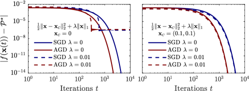
Refer to caption
Figure 11: Comparison of SGD and AGD on (61) with 𝒙C=0subscript𝒙C0{{\bm{x}}_{\textrm{C}}}=0 on the left and with 𝒙C=(0.1,0.1)subscript𝒙C0.10.1{{\bm{x}}_{\textrm{C}}}=(0.1,0.1) on the right.

References

  • [1] M. E. Baran and F. F. Wu. Optimal capacitor placement on radial distribution systems. IEEE Trans. on Power Delivery, 4(1):725–734, 1989.
  • [2] Mokhtar S Bazaraa, Hanif D Sherali, and C M Shetty. Nonlinear programming: Theory and algorithms. John Wiley & Sons, Chichester, England, 3 edition, 2006.
  • [3] D. Bertsekas and J. Tsitsiklis. Parallel and Distributed Computation: Numerical Methods. Prentice-Hall, 1989.
  • [4] J Frédéric Bonnans and Alexander Shapiro. Perturbation analysis of optimization problems. Springer Science & Business Media, 2013.
  • [5] Subhonmesh Bose, Dennice F Gayme, K Mani Chandy, and Steven H Low. Quadratically constrained quadratic programs on acyclic graphs with application to power flow. IEEE Trans. on Control of Network Systems, 2(3):278–287, 2015.
  • [6] Subhonmesh Bose, Hoa Dinh Nguyen, Haitian Liu, Ye Guo, Thinh T Doan, and Carolyn L Beck. Distributed dual subgradient methods with averaging and applications to grid optimization. arXiv preprint arXiv:2107.07061, 2021.
  • [7] Stephen Boyd, Lin Xiao, Almir Mutapcic, and Jacob Mattingley. Notes on decomposition methods. Notes for EE364B, Stanford University, 635:1–36, 2007.
  • [8] Sébastien Bubeck. Convex Optimization: Algorithms and Complexity. Foundations and Trends® in Machine Learning, 8(3-4):231–357, 2015.
  • [9] Mary B Cain, Richard P O’Neill, Anya Castillo, et al. History of optimal power flow and formulations. Federal Energy Regulatory Commission, 1:1–36, 2012.
  • [10] E. DallAnese, S. Guggilam, A. Simonetto, Y. C. Chen, and S. V. Dhople. Optimal regulation of virtual power plants. IEEE Trans. on Power Systems, 33(2):1868–1881, 2018.
  • [11] Thinh T Doan, Subhonmesh Bose, D Hoa Nguyen, and Carolyn L Beck. Convergence of the iterates in mirror descent methods. IEEE Control Systems Letters, 3(1):114–119, 2018.
  • [12] John C Duchi, Alekh Agarwal, and Martin J Wainwright. Dual averaging for distributed optimization: Convergence analysis and network scaling. IEEE Trans. on Automatic control, 57(3):592–606, 2011.
  • [13] M. Farivar and S. H. Low. Branch flow model: Relaxations and convexification (parts I, II). IEEE Trans. on Power Systems, 28(3):2554–2572, 2013.
  • [14] Lingwen Gan, Na Li, Ufuk Topcu, and Steven H Low. Exact convex relaxation for optimal power flow in distribution networks. IEEE Trans. on Automatic Control, 60(1):351–352, 2015.
  • [15] Y. Guo, S. Bose, and L. Tong. On robust tie-line scheduling in multi-area power systems. IEEE Trans. on Power Systems, 33(4):4144–4154, 2018.
  • [16] Emil Gustavsson, Michael Patriksson, and Ann-Brith Strömberg. Primal convergence from dual subgradient methods for convex optimization. Mathematical Programming, 150(2):365–390, 2015.
  • [17] R.A. Horn and C.R. Johnson. Matrix Analysis. Cambridge, U.K.: Cambridge Univ. Press, 1985.
  • [18] Hsu Kao and Vijay Subramanian. Convergence rate analysis for distributed optimization with localization. In 2019 57th Annual Allerton Conference on Communication, Control, and Computing (Allerton), pages 384–390. IEEE, 2019.
  • [19] B. H. Kim and R. Baldick. Coarse-grained distributed optimal power flow. IEEE Trans. on Power Systems, 12(2):932–939, May 1997.
  • [20] Torbjörn Larsson, Michael Patriksson, and Ann-Brith Strömberg. Ergodic, primal convergence in dual subgradient schemes for convex programming. Mathematical programming, 86(2):283–312, 1999.
  • [21] Javad Lavaei and Steven H Low. Zero duality gap in optimal power flow problem. IEEE Trans. on Power Systems, 27(1):92–107, 2011.
  • [22] Shu Liang, Le Yi Wang, and George Yin. Distributed dual subgradient algorithms with iterate-averaging feedback for convex optimization with coupled constraints. IEEE Trans. on Cybernetics, 2019.
  • [23] Steven H Low. Convex relaxation of optimal power flow—part II: Exactness. IEEE Trans. on Control of Network Systems, 1(2):177–189, 2014.
  • [24] Jing Ma et al. Recovery of primal solution in dual subgradient schemes. PhD thesis, Massachusetts Institute of Technology, 2007.
  • [25] Avinash N Madavan and Subhonmesh Bose. A stochastic primal-dual method for optimization with conditional value at risk constraints. Journal of Optimization Theory and Applications, 190(2):428–460, 2021.
  • [26] Ion Necoara and Valentin Nedelcu. On linear convergence of a distributed dual gradient algorithm for linearly constrained separable convex problems. Automatica, 55:209–216, May 2015.
  • [27] A. Nedić and A. Ozdaglar. Distributed subgradient methods for multi-agent optimization. IEEE Trans. on Automatic Control, 54(1):48–61, 2009.
  • [28] Angelia Nedić and Asuman Ozdaglar. Approximate primal solutions and rate analysis for dual subgradient methods. SIAM Journal on Optimization, 19(4):1757–1780, 2009.
  • [29] Y. Nesterov. Introductory Lectures on Convex Optimization: A Basic Course. Kluwer Academic Publishers, Norwell, MA, 2004.
  • [30] Yu Nesterov and Vladimir Shikhman. Dual subgradient method with averaging for optimal resource allocation. European Journal of Operational Research, 270(3):907–916, 2018.
  • [31] Giuseppe Notarstefano, Ivano Notarnicola, and Andrea Camisa. Distributed Optimization for Smart Cyber-Physical Networks. Foundations and Trends® in Systems and Control, 7(3):253–383, 2020.
  • [32] BT Polyak. Introduction to optimization. Translations Series in Mathematics and Engineering. New York: Optimization Software Inc. Publications Division, 1987.
  • [33] Guannan Qu and Na Li. Accelerated Distributed Nesterov Gradient Descent. IEEE Transactions on Automatic Control, 65(6):2566–2581, June 2020.
  • [34] Andrea Simonetto and Hadi Jamali-Rad. Primal recovery from consensus-based dual decomposition for distributed convex optimization. Journal of Optimization Theory and Applications, 168(1):172–197, 2016.
  • [35] Brian Stott, Jorge Jardim, and Ongun Alsaç. DC power flow revisited. IEEE Trans. on Power Systems, 24(3):1290–1300, 2009.
  • [36] Di Wu, Jianming Lian, Yannan Sun, Tao Yang, and Jacob Hansen. Hierarchical control framework for integrated coordination between distributed energy resources and demand response. Electric Power Systems Research, 150:45–54, September 2017.
  • [37] Baosen Zhang and David Tse. Geometry of injection regions of power networks. IEEE Trans. on Power Systems, 28(2):788–797, 2012.
  • [38] X. Zhou, E. Dall’Anese, L. Chen, and A. Simonetto. An incentive-based online optimization framework for distribution grids. IEEE Trans. on Automatic Control, 2017.