Mitigating Memorization in Sample Selection for Learning with Noisy Labels

Abstract

Because deep learning is vulnerable to noisy labels, sample selection techniques, which train networks with only clean labeled data, have attracted a great attention. However, if the labels are dominantly corrupted by few classes, these noisy samples are called dominant-noisy-labeled samples, the network also learns dominant-noisy-labeled samples rapidly via content-aware optimization. In this study, we propose a compelling criteria to penalize dominant-noisy-labeled samples intensively through class-wise penalty labels. By averaging prediction confidences for the each observed label, we obtain suitable penalty labels that have high values if the labels are largely corrupted by some classes. Experiments were performed using benchmarks (CIFAR-10, CIFAR-100, Tiny-ImageNet) and real-world datasets (ANIMAL-10N, Clothing1M) to evaluate the proposed criteria in various scenarios with different noise rates. Using the proposed sample selection, the learning process of the network becomes significantly robust to noisy labels compared to existing methods in several noise types.

1 Introduction

For training deep neural networks (DNNs) using a supervised learning method, the labeled data are predominantly obtained from web queries (Liu et al., 2011), crowdsourcing (Welinder et al., 2010; Han et al., 2018a; Yan et al., 2014), e-commerce (Xiao et al., 2015) and social-network (Cha & Cho, 2012). However, several noisy labeled samples (In this study, we omit “labeled” for brevity) that are annotated with erroneous or noisy labels are present in the data. Zhang (Zhang et al., 2016) confirmed that a DNN is significantly vulnerable to noisy samples because it can adequately learn (memorize) their patterns. To robustly train a network regardless of noisy samples, learning with noisy labels has been studied actively. These studies can be divided into two categories based on the technique employed: loss correction and sample selection.

In the loss correction category, the loss (or label) of a mini-batch is modified using a noise transition matrix (Goldberger & Ben-Reuven, 2016; Patrini et al., 2017; Han et al., 2018b; Hendrycks et al., 2018) or prediction confidences of samples (Reed et al., 2014; Chang et al., 2017; Tanaka et al., 2018; Ren et al., 2018; Wang et al., 2019b). However, if the number of classes or noise rate is large, the prediction confidences and noise transition matrix can be inaccurate (Han et al., 2018c; Song et al., 2019), leading to false correction and error accumulation in the training stage.

(a)

(b)

Figure 1: Comparison between (a) conventional and (b) proposed algorithms based on robust sample selection. In mini-batch $\mathcal{B}$, for clear visualization, we only represent samples which have a single observed label among various observed labels. In Criteria with Observed Label (Criteria_OL) and Criteria with Penalty Label (Criteria_PL), inner product of prediction confidence of each sample and the label is performed. Furthermore, $P_{i}$ represents the prediction confidence in the $i$th class. In the sample selection stage, the conventional algorithm using Criteria_OL selects lots of dominant noisy samples as well as clean samples. In contrast, the proposed algorithm using Criteria_ALL, which subtracts a proposed Criteria_PL from Criteria_OL, rarely selects dominant noisy samples because dominant noisy samples can be penalized appropriately through Criteria_PL with proposed penalty label. Thereafter, both algorithms updates network parameters using the selected samples with their observed labels.

Recently, to overcome this limitation, many studies have been based on the sample selection method. In the sample selection category, only clean samples, whose labels are accurate, are selected from the mini-batch and thereafter used to train the network (Han et al., 2018c; Malach & Shalev-Shwartz, 2017; Wang et al., 2019a; Yu et al., 2019; Shen & Sanghavi, 2019; Song et al., 2019; Kong et al., 2019)‘. They are based on “content-aware optimization” (also called “memorization effect”), wherein it initially learns simple patterns shared by multiple training samples across the data regardless of their labels (Arpit et al., 2017). Using this characteristic, sample selection based algorithms (Fig. 1a) assume that the DNN initially learns clean samples more rapidly than noisy ones. Therefore, the algorithms first select samples which have high scores (low losses) using observed labels that include noisy labels, then, train the DNN using the selected samples.

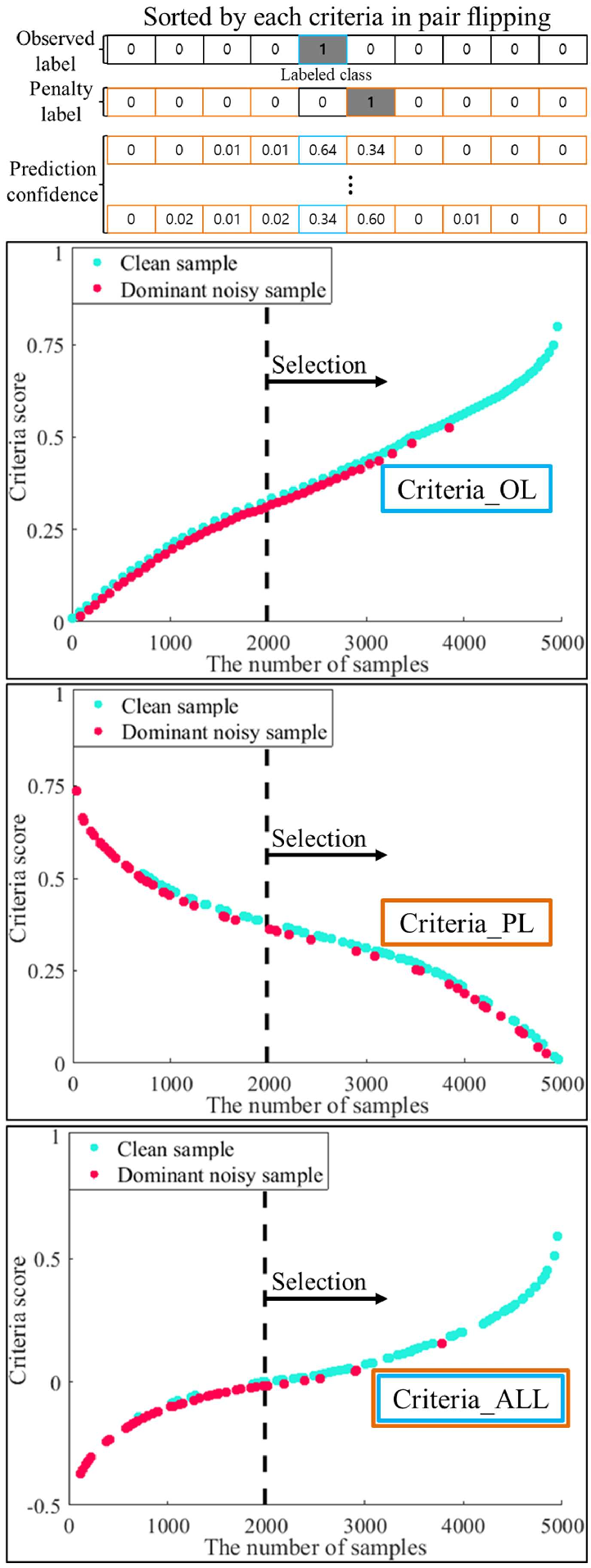
However, the performances of the sample selection algorithms vary depending on types of noise. If the labels are dominantly corrupted by some classes, noisy samples generally have shared patterns and can also be learned rapidly by content-aware optimization (we call these noisy samples dominant noisy samples). Thus, dominant noisy samples have high score with observed labels, thus selection algorithms can not exclude these samples. In Fig. 1(a), many dominant noisy samples are selected for training DNN because dominant noisy samples have higher scores than the other noisy samples and some clean samples. They cause severe memorization of DNN, so it is important to penalize dominant noisy samples in sample selection.

In this study, we introduce Criteria_ALL, which subtracts new Criteria with the proposed Penalty Label (Criteria_PL) from the conventional Criteria_OL with the observed label for penalizing dominant noisy samples (Fig. 1b). In the proposed Criteria_PL with penalty label, dominant noisy samples have higher scores than the non-dominant ones and clean samples. Therefore, Criteria_ALL is effective for penalizing dominant noisy samples (Fig. 1b; red samples). To estimate the penalty label, we use the average-prediction confidence of samples that belong to identical observed label after normalizing the result (Section 2.2; Fig. 2). In summary, the main contributions of this study are the following:

• We observe that dominant noisy samples cause memorization (reduce generalization) of DNN through empirical evidence.

• We propose a new Criteria_PL that have high criteria scores for dominant noisy samples, and can penalize dominant noisy samples by subtracting Criteria_PL from the conventional Criteria_OL (Criteria_ALL).

2 Main methodology: penalizing dominant noisy samples in sample selection

In this section, we describe our sample selection method to achieve robust learning in detail.

2.1 Sample selection with conventional Criteria_OL

In the $K$-class classification problem, let ${\mathcal{D}=\left\{\left({\mathbf{x}}_{i},{\hat{\mathbf{y}}}_{i}\right)\right\}}_{i=1}^{n}$ be training dataset, where ${\mathbf{x}}_{i}$ is the $i$th sample and ${\hat{\mathbf{y}}}_{i}$ is the $i$th observed label that includes corrupted label and is in the label space $\left\{{\mathbf{e}}^{k}:k\in\left\{1,2,\cdots,K\right\}\right\}$, i.e., ${\mathbf{e}}^{k}$:$k$th one-hot vector such as $\left[0,\cdots,0,1,0,\cdots,0\right]$. The objective is to train the DNN parameter $\bm{\theta}$ through the maximum likelihood estimation ${\mathrm{argmax}}_{\bm{\theta}}\sum_{i=1}^{n}P\left({\hat{\mathbf{y}}}_{i}|{\mathbf{x}}_{i};\bm{\theta}\right)$. Herein, the prediction confidence in $j$th class, which indicates the probability of being assigned to $j$th class (probability for the label $\mathbf{e}^{j}$), is obtained by applying a softmax function to the DNN $f$:

$$P\left(\mathbf{y}=\mathbf{e}^{j}|{\mathbf{x}}_{i};\bm{\theta}\right)=\frac{\exp\left\{{f\left({\mathbf{x}}_{i}\right)}_{j}\right\}}{\sum_{l=1}^{K}\exp\left\{{f\left({\mathbf{x}}_{i}\right)}_{l}\right\}},\forall j=1,\cdots,K,$$

where ${f\left(\cdot\right)}_{j}$ is $j$th component of $f\left(\cdot\right)$. The loss function is generally defined by the cross-entropy scheme with the observed label ${\mathbf{\hat{\mathbf{y}}}_{i}}$ and prediction $P\left(\mathbf{y}=\mathbf{e}^{j}|{\mathbf{x}}_{i};\bm{\theta}\right)$:

$$\mathcal{L}\left({\mathbf{x}}_{i},{\hat{\mathbf{y}}}_{i};\bm{\theta}\right)=-\log P\left(\mathbf{y}={\hat{\mathbf{y}}}_{i}|{\mathbf{x}}_{i};\bm{\theta}\right).$$ (1)

DNN is trained through a stochastic optimization method, which updates the parameter $\bm{\theta}$ using the mini-batch procedure:

$${\bm{\theta}}^{t+1}={\bm{\theta}}^{t}-\eta\nabla\left(\frac{1}{\left|\mathcal{B}\right|}\sum_{\left({\mathbf{x}}_{i},{\hat{\mathbf{y}}}_{i}\right)\in\mathcal{B}}\mathcal{L}\left({\mathbf{x}}_{i},{\hat{\mathbf{y}}}_{i};{\bm{\theta}}^{t}\right)\right),$$ (2)

where ${\bm{\theta}}^{t}$ is a parameter in the $t$th iteration, $\eta$ is the learning rate, and $\mathcal{B}$ is the mini-batch fetched from $\mathcal{D}$.

Recently, several algorithms based on sample selection method (Han et al., 2018c; Jiang et al., 2018; Wang et al., 2019a; Yu et al., 2019) have been developed to robustly train the DNN for noisy labels. These methods assume that clean samples are trained more easily compared with the noisy samples, because DNN is trained by content-aware optimization wherein it initially learns simple patterns shared among multiple samples (Arpit et al., 2017). Therefore, in a mini-batch manner, sample selection methods select top $R\%$ of sorted samples in descending order relative to probability for the observed label (Fig. 1a). Then the network parameter is updated using only selected samples as

$${\bm{\theta}}^{t+1}={\bm{\theta}}^{t}-\eta\nabla\left(\frac{1}{\left|{\mathcal{S}}\right|}\sum_{\left({\mathbf{x}}_{i},{\hat{\mathbf{y}}}_{i}\right)\in{\mathcal{S}}}\mathcal{L}\left({\mathbf{x}}_{i},{\hat{\mathbf{y}}}_{i};{\bm{\theta}}^{t}\right)\right),$$ (3)

where

$${\mathcal{S}} ={\mathrm{SELECT}}_{\left({\mathbf{x}}_{i},{\hat{\mathbf{y}}}_{i}\right)\in{\mathcal{B}}}^{\mathrm{TOP}\,R\%}\sum_{j=1}^{K}{\hat{\mathbf{y}}}_{i}\left(j\right)P\left(\mathbf{y}={\mathbf{e}}^{j}|{\mathbf{x}}_{i};{\bm{\theta}}^{t}\right),$$ (4)

where ${\mathrm{TOP}\,R\%}$ means top $R\%$ of sorted samples in descending order, ${\hat{\mathbf{y}}}_{i}\left(\cdot\right)$ is an element of one-hot vector ${\hat{\mathbf{y}}}_{i}$, $R\%=100-\varepsilon$, and $\varepsilon$ is the percentage of noise label. It is based on selection criteria, Criteria_OL, where “sample should have high prediction confidence for observed label” as follows:

$${\mathrm{{Criteria}\_{OL}}\left({\mathbf{x}}_{i},{\hat{\mathbf{y}}}_{i};{\bm{\theta}}^{t}\right)=\sum_{j=1}^{K}{\hat{\mathbf{y}}}_{i}\left(j\right)P\left(\mathbf{y}={\mathbf{e}}^{j}|{\mathbf{x}}_{i};{\bm{\theta}}^{t}\right)}.$$

However, if the labels are largely corrupted by some classes, these samples have high probability of having several shared patterns among themselves, like clean labels data. Therefore, dominant noisy samples can also be included in selected samples, causing memorization (reducing generalization) of DNN (empirical evidence is provided in Section 3.1).

2.2 Criteria_ALL: combination of proposed Criteria_PL and Criteria_OL

To penalize dominant noisy samples, we propose the criteria, Criteria_PL, which exploits proposed penalty label. In Criteria_PL, dominant noisy samples have higher values than the non-dominants. This is because the penalty label is set to have high values in the classes where dominant noisy samples originate; moreover, (dominant) noisy samples generally have high prediction confidences in their true class. Therefore, to penalize dominant noisy samples, we introduce a selection criteria (Criteria_ALL) by subtracting Criteria_PL “sample should have high prediction confidence for proposed penalty label $\tilde{\mathbf{y}}$” from Criteria_OL as follows:

$$\mathrm{{Criteria}\_{ALL}}=\mathrm{{Criteria}\_{OL}}-\lambda\>\mathrm{{Criteria}\_{PL}},$$ (5)

where

$${\mathrm{{Criteria}\_{OL}}\left({\mathbf{x}}_{i},{\hat{\mathbf{y}}}_{i};{\bm{\theta}}^{t}\right)=\sum_{j=1}^{K}{\hat{\mathbf{y}}}_{i}\left(j\right)P\left(\mathbf{y}={\mathbf{e}}^{j}|{\mathbf{x}}_{i};{\bm{\theta}}^{t}\right)},$$

$$\mathrm{{Criteria}\_{PL}}\left({\mathbf{x}}_{i},{\tilde{\mathbf{y}}}_{i};{\bm{\theta}}^{t}\right)=\sum_{j=1}^{K}{\tilde{\mathbf{y}}}_{i}\left(j\right)P\left(\mathbf{y}=\mathbf{e}^{j}|{\mathbf{x}}_{i};{\bm{\theta}}^{t}\right),$$

where $\lambda$ is hyperparameter (user design parameter) and ${\tilde{\mathbf{y}}}_{i}\left(\cdot\right)$ is an element of $i$th penalty label. The effectiveness of Criteria_PL is described in detail with empirical evidence in Section 3.1.

Figure 2: Process of acquiring penalty label ${\tilde{\mathbf{y}}}$: this process is conducted for each observed label ${\hat{\mathbf{y}}}=\mathbf{e}^{k}$ in the same manner.

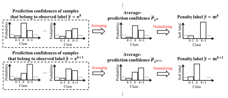
To penalize dominant noisy samples through the proposed Criteria_ALL, it is necessary to estimate the penalty label properly. The process to obtain class-wise penalty label ${\tilde{\mathbf{y}}}$ is shown in Fig. 2. First, we average the prediction confidences among samples that have same observed label ${C}^{k}=\left\{\left({\mathbf{x}}_{i},{\hat{\mathbf{y}}}_{i}\right):\hat{\mathbf{y}}_{i}=\mathbf{e}^{k}\right\}$ to measure the extent of dominance of the noisy samples. This method is reasonable because the percentage of noisy samples that are dominant is high; the dominant noisy samples have high prediction confidence in their true class (this will be shown in Section 3.1). Finally, to ensure the same scale with observed labels, the compensated average-prediction confidence is normalized except the class that the observed label $\hat{\mathbf{y}}=\mathbf{e}^{k}$ indicates (labeled class $k$). This is because samples in labeled class $k$ are not needed to be penalized.

The penalty label $\tilde{\mathbf{y}}_{i}\in\left\{{\mathbf{m}}^{k}:k\in\left\{1,2,\cdots,K\right\}\right\}$ is defined by

$${\mathbf{m}}^{k}\left(j\right)=\begin{cases}\dfrac{1}{A}{\bar{P}}_{{C}^{k}}\left(\mathbf{y}=\mathbf{e}^{j}|{\bm{\theta}}^{t}\right),&\text{ if }\;j\neq k\\ 0,&\text{ if }\;j=k\end{cases},$$ (6)

where

$$A=\sum_{l\neq k}{\bar{P}}_{{C}^{k}}\left(\mathbf{y}=\mathbf{e}^{l}|{\bm{\theta}}^{t}\right),$$ (7)

$${{\bar{P}}_{{C}^{k}}\left(\mathbf{y}=\mathbf{e}^{j}|{\bm{\theta}}^{t}\right)=\sum_{\left({\mathbf{x}}_{i},{\hat{\mathbf{y}}}_{i}\right)\in{C}^{k}}{P}\left(\mathbf{y}=\mathbf{e}^{j}|{\mathbf{x}}_{i};\bm{\theta}^{t}\right)},$$ (8)

where ${C}^{k}$ is $\left\{\left({\mathbf{x}}_{i},{\hat{\mathbf{y}}}_{i}\right):\hat{\mathbf{y}}_{i}=\mathbf{e}^{k}\right\}$.

Algorithm 1 Sample selection with Criteria_ALL.

1:for $t=1:num\_epochs$ do

2:     for $l=1:num\_iterations$ do

3:         Predict mini-batch ${\mathcal{B}}$;

4:         Stack prediction confidences $P$;

5:         Select samples ${\mathcal{S}}_{Prop}$ from mini-batch ${\mathcal{B}}$ within

6:               top $R\%$ using $\mathrm{Criteria\_ALL}$;

7:         Update network using selected samples ${\mathcal{S}}_{Prop}$;

8:     end for

9:     Update penalty label $\tilde{\mathbf{y}}^{t}$;

10:end for

Finally, the network is trained with samples selected using Criteria_ALL by

$${{\mathcal{S}}}_{Prop} ={\mathrm{SELECT}}_{\left({\mathbf{x}}_{i},{\hat{\mathbf{y}}}_{i}\right)\in{\mathcal{B}}}^{\mathrm{TOP}\,R\%}\mathrm{{Criteria}\_{ALL}}\left({\mathbf{x}}_{i},{\hat{\mathbf{y}}}_{i},{\tilde{\mathbf{y}}}_{i};{\bm{\theta}}^{t}\right).$$ (9)

Algorithm 1 describes the overall procedure of sample selection with Criteria_ALL. The penalty label is updated at the end of each epoch (in step 9 of Algorithm 1).

(a)

(b)

Figure 3: When the sample selection is performed with pair and mixed flipping noise, the results are represented by sorted samples in each criteria. The samples on the right-hand side of the black dashed line are selected. For clear visualization, we only show samples that have same observed label $\hat{\mathbf{y}}=\mathbf{e}^{5}$ on CIFAR-10 in initial training. Furthermore, we conduct down-sampling by interval 40, then depict these ones sorting for each criteria. The Criteria_ALL and Criteria_OL are sorted in ascending order, and the Criteria_PL is sorted in descending order. (a) Pair flipping (Han et al., 2018c): the true labels of class 5 are corrupted by the labels of class 6 with the noise rate of 40%. (b) Mixed flipping: the true labels of class 5 are corrupted by the labels of class 6 with the noise rate of 24% and the other classes at a same noise rate of 2% (total 40%).

3 Deep understanding for Criteria_ALL

In this section, we mainly describe the effectiveness of Criteria_ALL based on empirical evidence on CIFAR-10 dataset (Krizhevsky et al., 2009).

3.1 Why Criteria_OL and Criteria_PL are necessary?

We explain the validity of Criteria_ALL with respect to the following two points.

1. Which noisy samples should be penalized in sample selection with Criteria_OL?

2. How can Criteria_PL penalize noisy samples using the proposed penalty label?

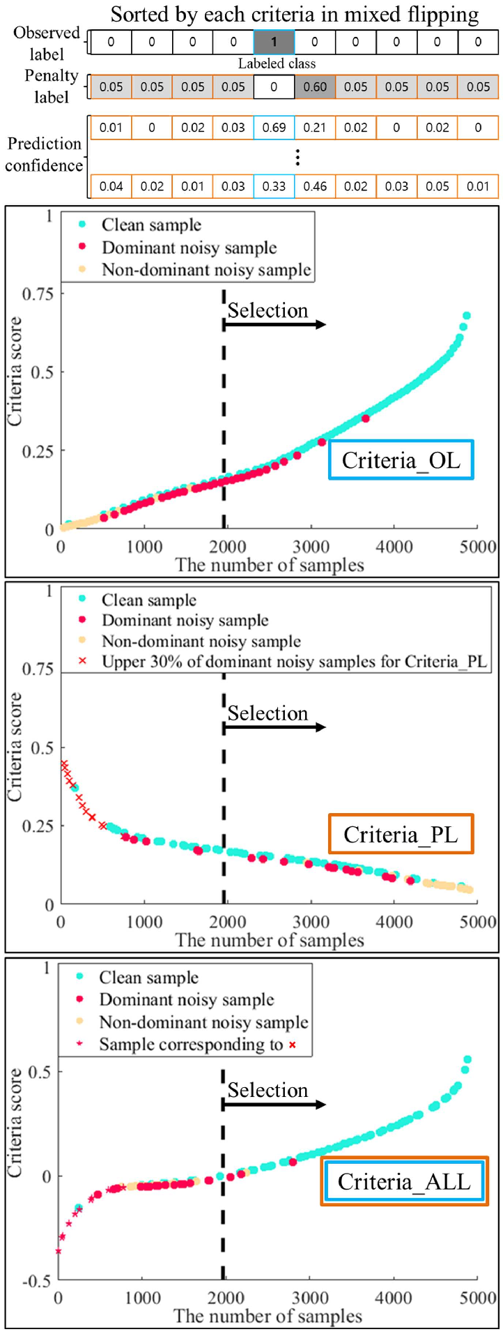
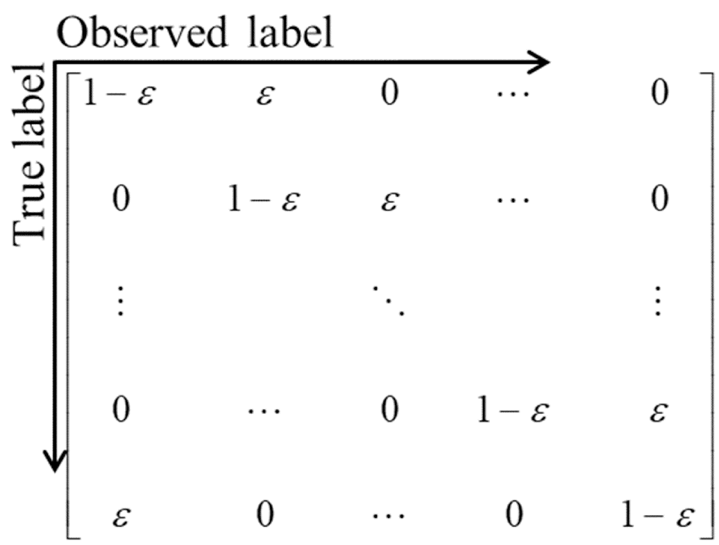
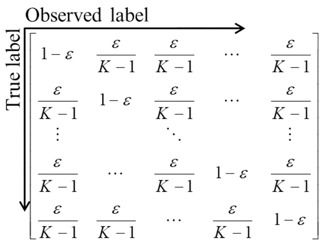
First, when the labels are significantly corrupted by certain classes (pair $>$ mixed $>$ symmetry in Fig. 4), dominant noisy samples generally have shared patterns with themselves, and thus can also be learned rapidly by content-aware optimization. In pair flipping, because noisy samples are corrupted by a single class (all noisy samples are dominant), several noisy samples are included in the selected samples (Fig. 3a top panel; red circles on the right-hand side of the black dashed line). In mixed flipping, noisy samples originate in several classes and can be dominant or non-dominant depending on their proportion. Because dominant noisy samples have considerable shared patterns compared to the non-dominants, the dominants are trained more rapidly than the non-dominants by content-aware optimization; consequently, some noisy samples among dominant noisy samples are included in selected samples (Fig. 3b top panel; red solid circles on the right-hand side of the black dashed line). Therefore, dominant noisy samples cause memorization (reduce generalization) of DNN, and it is important to penalize them in sample selection.

Thereafter, we focus on how Criteria_PL can penalize dominant noisy samples using penalty labels. For general noisy label distributions (e.g., mixed flipping case), because dominant noisy samples cause significant memorization than non-dominant ones, we propose a novel class-wise penalty label that reflects extent of dominance for penalizing noisy samples differently. When the penalty label and prediction confidence of each sample are multiplied by inner product, then the dominant noisy samples will have higher values than that of the non-dominants. This is because (dominant) noisy samples generally have high prediction confidence in their true class, and the penalty label is set to have relatively higher value in the class, which dominant noisy samples originates, than the other classes. Therefore, we can distinguish dominant noisy sample using the proposed criteria, Criteria_PL, defined by inner product of penalty label and prediction confidence of each sample. In Fig. 3(b), because penalty label is set to have a relatively high value (e.g., sixth value in penalty label: 0.60) in class 6 where dominant noisy samples originate, and prediction confidences of dominant noisy samples also have the highest value (e.g., sixth value in last prediction confidence: 0.46) in class 6 (its true class), most dominant noisy samples have higher criteria scores than clean and non-dominant samples in Criteria_PL (middle panel). Finally, we subtract the Criteria_PL from Criteria_OL (defined as Criteria_ALL) for penalizing dominant noisy samples largely. Using Criteria_ALL, penalized dominant and non-dominant noisy samples have smaller criteria scores compared to most clean samples and have similar criteria scores with each other (Fig. 3(b) bottom panel). Lastly, in symmetry flipping case, Criteria_PL does not affect the selection of clean samples because of no dominant noisy samples (proofed in Appendix C).

4 Experiments

We evaluate the effect of the proposed Criteria_ALL with regard to two perspectives. First, we evaluate the performance using three benchmark datasets by corrupting clean labels using three different type of noisy label with various noise rates. Second, we evaluate the performance using two real-world datasets (Appendix B.5). Three independent trials were performed and average and standard error are used to represent the performance of the proposed, and conventional algorithms. Dataset are described in (Appendix B.2).

(a)

(b)

(c)

Figure 4: Several noise types; (a) Pair flipping; (b) Symmetry flipping; (c) Mixed flipping ($\varepsilon=\varepsilon_{1}+\varepsilon_{2}$).

(a)

(b)

(c)

Figure 5: Best test error (%) based on various noise rates with pair flipping; (a) CIFAR-10; (b) CIFAR-100; (c) Tiny-ImageNet.

4.1 Algorithms

We compared Criteria_ALL with several algorithms in the loss correction and sample selection categories. Default (baseline) was network that was trained without processing for noisy labels. Active Bias (Chang et al., 2017) (loss correction) trained DNN by assigning large weights to uncertain samples that exhibit high variance. MentorNet (Jiang et al., 2018) (sample selection) used Criteria_OL to select clean samples and trains DNN using only selected samples. Co-teaching (Han et al., 2018c) (sample selection) used two networks and exchanged information of sample selection to enhance the difference. Co-teaching+ (sample selection) applied Co-teaching to the samples with different prediction confidence. SL (Wang et al., 2019b) (loss correction) combined reverse cross entropy term with cross entropy loss to enhance cross entropy’s learning on hard classes and tolerance to noisy labels. SELFIE (Song et al., 2019) (hybrid) corrected loss of samples with high precision while conducting the conventional sample selection. MentorNet–Prop is a basic sample selection method that uses Criteria_ALL rather than Criteria_OL. Because Criteria_ALL can be applied flexibly to other algorithms, we also conducted experiments using SL–Prop and SELFIE–Prop by combining Criteria_ALL with SL and SELFIE (Appendix A.2).

Table 1: Best test error (%) with different noise rates for each noise type

	Default	Active Bias	Co-teaching	Co-teaching+	SL	SELFIE	MentorNet–Prop	SL–Prop	SELFIE–Prop
Sample selection	$\times$	$\times$	$\bigcirc$	$\bigcirc$	$\times$	$\bigcirc$	$\bigcirc$	$\bigcirc$	$\bigcirc$
Loss correction	$\times$	$\bigcirc$	$\times$	$\times$	$\bigcirc$	$\bigcirc$	$\times$	$\bigcirc$	$\bigcirc$

Dataset	Method	Pair flipping				Symmetry flipping				Mixed
		Noise rate $\varepsilon$				Noise rate $\varepsilon$				Noise rate $\varepsilon$
		10%	20%	30%	40%	0%	20%	40%	60%	40%
CIFAR- 10	Default	10.2$\pm$0.24	11.8$\pm$0.03	13.6$\pm$0.07	18.4$\pm$0.35	8.6$\pm$0.07	13.2$\pm$0.08	17.4$\pm$0.25	25.7$\pm$0.55	16.0$\pm$0.16
	Active Bias	9.5$\pm$0.08	10.8$\pm$0.13	12.1$\pm$0.09	17.6$\pm$0.33	8.5$\pm$0.09	12.2$\pm$0.16	15.7$\pm$0.39	24.2$\pm$0.21	14.4$\pm$0.23
	Co-teaching	10.0$\pm$0.09	11.3$\pm$0.13	12.7$\pm$0.01	15.3$\pm$0.30	8.8$\pm$0.05	11.0$\pm$0.01	14.1$\pm$0.18	19.4$\pm$0.12	14.4$\pm$0.36
	Co-teaching+	12.4$\pm$0.13	14.0$\pm$0.21	15.8$\pm$0.22	23.1$\pm$2.17	11.2$\pm$0.25	13.7$\pm$0.17	17.2$\pm$0.30	33.5$\pm$1.90	17.9$\pm$0.49
	SL	10.2$\pm$0.12	11.2$\pm$0.03	13.7$\pm$0.20	18.3$\pm$0.46	8.5$\pm$0.04	12.6$\pm$0.17	17.0$\pm$0.32	25.6$\pm$0.16	16.2$\pm$0.15
	SELFIE	9.5$\pm$0.10	10.6$\pm$0.08	11.5$\pm$0.05	13.3$\pm$0.08	8.7$\pm$0.09	10.9$\pm$0.01	13.5$\pm$0.04	20.5$\pm$0.23	13.3$\pm$0.17
	MentorNet–Prop	9.5$\pm$0.05	10.5$\pm$0.04	11.1$\pm$0.04	12.2$\pm$0.12	8.6$\pm$0.05	11.1$\pm$0.11	14.4$\pm$0.26	20.5$\pm$0.11	13.4$\pm$0.11
	SL–Prop	9.3$\pm$0.13	10.2$\pm$0.07	10.8$\pm$0.18	11.7$\pm$0.13	8.6$\pm$0.13	11.0$\pm$0.07	13.7$\pm$0.03	19.9$\pm$0.08	13.2$\pm$0.23
	SELFIE–Prop	8.9$\pm$0.13	9.7$\pm$0.07	10.8$\pm$0.12	11.7$\pm$0.11	8.4$\pm$0.09	10.5$\pm$0.02	13.7$\pm$0.10	20.4$\pm$0.10	13.0$\pm$0.11
CIFAR- 100	Default	34.9$\pm$0.29	37.4$\pm$0.13	43.6$\pm$0.49	53.2$\pm$0.46	31.7$\pm$0.18	37.5$\pm$0.18	43.5$\pm$0.21	53.8$\pm$0.08	47.6$\pm$0.71
	Active Bias	34.1$\pm$0.32	36.6$\pm$0.16	40.9$\pm$0.27	50.8$\pm$0.08	31.1$\pm$0.31	36.6$\pm$0.28	42.1$\pm$0.29	52.9$\pm$0.19	44.8$\pm$0.14
	Co-teaching	33.2$\pm$0.20	36.2$\pm$0.13	41.4$\pm$0.15	51.8$\pm$0.75	31.9$\pm$0.16	34.3$\pm$0.11	37.5$\pm$0.01	44.3$\pm$0.57	45.7$\pm$0.42
	Co-teaching+	35.6$\pm$0.17	37.2$\pm$0.17	40.3$\pm$0.18	47.3$\pm$0.20	33.8$\pm$0.19	36.2$\pm$0.15	40.6$\pm$0.21	49.1$\pm$0.31	43.7$\pm$0.18
	SL	34.1$\pm$0.14	36.5$\pm$0.08	42.0$\pm$0.42	52.3$\pm$0.59	31.1$\pm$0.05	36.5$\pm$0.30	42.7$\pm$0.23	52.4$\pm$0.53	45.7$\pm$0.23
	SELFIE	32.7$\pm$0.09	34.1$\pm$0.12	35.8$\pm$0.18	41.3$\pm$0.15	31.7$\pm$0.05	33.8$\pm$0.08	37.1$\pm$0.02	44.6$\pm$0.13	38.5$\pm$0.16
	MentorNet–Prop	32.5$\pm$0.04	33.8$\pm$0.19	34.6$\pm$0.20	36.6$\pm$0.11	31.3$\pm$0.16	34.6$\pm$0.10	38.3$\pm$0.11	45.4$\pm$0.34	37.8$\pm$0.23
	SL–Prop	32.4$\pm$0.11	33.3$\pm$0.11	34.4$\pm$0.09	36.2$\pm$0.40	31.1$\pm$0.23	34.4$\pm$0.07	38.0$\pm$0.11	46.0$\pm$0.63	37.2$\pm$0.42
	SELFIE–Prop	32.6$\pm$0.14	33.1$\pm$0.03	34.1$\pm$0.16	35.3$\pm$0.19	30.9$\pm$0.17	33.7$\pm$0.18	36.6$\pm$0.15	42.6$\pm$0.05	36.0$\pm$0.29
Tiny- ImageNet	Default	56.6$\pm$0.07	59.1$\pm$0.45	63.5$\pm$0.18	69.9$\pm$0.28	54.5$\pm$0.13	59.2$\pm$0.35	64.6$\pm$0.21	72.9$\pm$0.62	66.4$\pm$0.20
	Active Bias	56.6$\pm$0.05	58.9$\pm$0.12	62.1$\pm$0.29	68.2$\pm$0.06	55.0$\pm$0.23	58.7$\pm$0.11	64.1$\pm$0.35	72.2$\pm$0.14	65.0$\pm$0.01
	Co-teaching	56.3$\pm$0.13	59.0$\pm$0.15	63.7$\pm$0.38	71.5$\pm$0.19	54.9$\pm$0.07	56.9$\pm$0.29	60.9$\pm$0.13	65.7$\pm$0.08	66.8$\pm$0.12
	Co-teaching+	58.3$\pm$0.11	60.0$\pm$0.15	62.9$\pm$0.13	69.3$\pm$0.46	56.9$\pm$0.16	59.0$\pm$0.09	63.1$\pm$0.13	71.6$\pm$0.21	65.7$\pm$0.28
	SL	56.0$\pm$0.22	58.4$\pm$0.35	61.9$\pm$0.14	67.5$\pm$0.26	54.1$\pm$0.10	58.4$\pm$0.12	64.4$\pm$0.14	72.3$\pm$0.28	64.5$\pm$0.25
	SELFIE	56.1$\pm$0.19	57.9$\pm$0.11	59.7$\pm$0.06	64.7$\pm$0.08	54.7$\pm$0.19	56.4$\pm$0.22	60.3$\pm$0.08	69.4$\pm$0.19	63.3$\pm$0.18
	MentorNet–Prop	55.8$\pm$0.10	57.1$\pm$0.12	58.7$\pm$0.14	62.5$\pm$0.22	54.9$\pm$0.06	57.7$\pm$0.04	61.0$\pm$0.10	67.0$\pm$0.29	60.9$\pm$0.17
	SL–Prop	54.9$\pm$0.07	56.8$\pm$0.23	58.0$\pm$0.29	60.1$\pm$0.26	54.0$\pm$0.04	57.5$\pm$0.21	60.9$\pm$0.11	66.9$\pm$0.26	60.7$\pm$0.30
	SELFIE–Prop	55.5$\pm$0.04	56.8$\pm$0.13	57.6$\pm$0.20	60.5$\pm$0.21	54.1$\pm$0.10	57.1$\pm$0.12	59.7$\pm$0.21	64.0$\pm$0.01	60.1$\pm$0.17

4.2 Experimental results on benchmark datasets

Table 2: Best test error (%) in mixed flipping

Algorithm	CIFAR-10	CIFAR-100	Tiny-ImageNet
Default	16.0$\pm$0.16	47.6$\pm$0.71	66.4$\pm$0.20
MentorNet	15.2$\pm$0.27	46.7$\pm$0.54	66.9$\pm$0.24
MentorNet–Prop	13.4$\pm$0.11	37.8$\pm$0.23	60.9$\pm$0.17

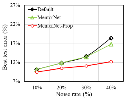
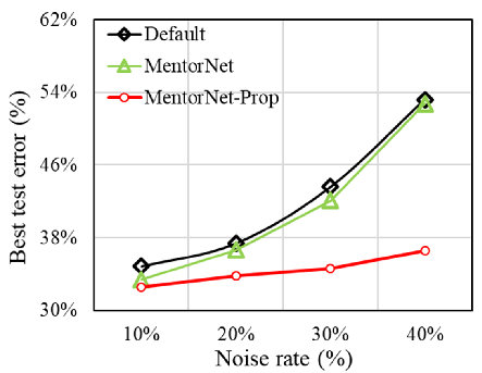
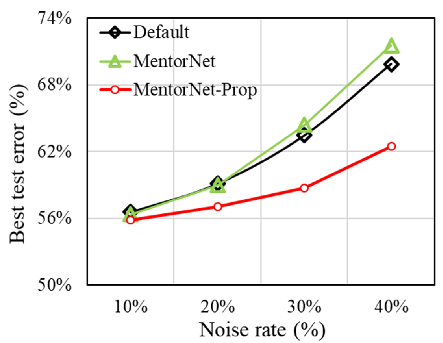
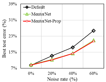
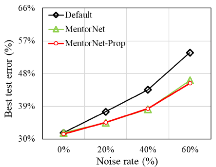
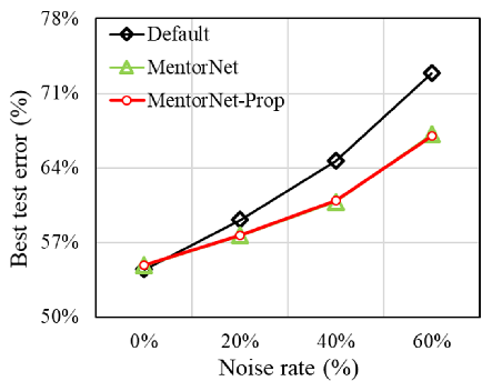
To examine the effect of the proposed Criteria_ALL in the sample selection category, we first compared the test errors of Default (without Criteria), MentorNet (with Criteria_OL), and MentorNet–Prop (with Criteria_ALL). In pair flipping, MentorNet–Prop presented the lowest test errors at all noise rates and for all datasets (Fig. 5), particularly when the noise rate was high. For mixed flipping, we conducted experiments with noise rate 40% (Table 2). Similar to pair flipping, MentorNet–Prop recorded the lowest test error in three datasets.

Thereafter, we compared MentorNet–Prop, SL–Prop, and SELFIE–Prop with conventional algorithms in the loss correction and sample selection categories with various noise rates. In Table 1 pair flipping, MentorNet–Prop displayed the overall lower test error compared to other conventional algorithms. Furthermore, SL–Prop and SELFIE–Prop achieved lowest test error. When the proposed Criteria_ALL is applied to SL, the test errors obtained were $0.9$–$16.1\%$ lower than those of SL. This means selecting sample using Criteria_ALL is also effective in loss correction category. SELFIE–Prop achieved test errors $0.1$–$6.0\%$ lower than those of SELFIE. In conclusion, when labels are corrupted as pair flipping, proposed Criteria_ALL is powerful.

The performances of the algorithms at various noise rates are also compared for the symmetry case in Table 1. MentorNet–Prop achieved lower or similar test errors as the conventional algorithms. Particularly, when the proposed Criteria_ALL is applied to SL, the test errors were $0.9$–$6.4\%$ lower than in SL. Experimental results show that Criteria_ALL is also effective in the loss correction category in symmetry flipping case. For mixed flipping case, MentorNet–Prop achieved lower or similar test errors to the conventional algorithms. Particularly, SELFIE–Prop had the lowest test errors.

5 Conclusion

To address learning with noisy labels, we introduced a novel criteria, Criteria_ALL that penalizing dominant noisy samples effectively by subtracting the proposed Criteria_PL from the conventional Criteria_OL. Because the penalty label reflects the extent of dominance of noisy samples, dominant noisy samples have higher criteria scores compared to non-dominant noisy samples and clean samples in Criteria_PL. Therefore, Criteria_ALL is effective for penalizing dominant noisy samples by subtracting Criteria_PL. From our experiments, sample selection using the Criteria_ALL was effective for several benchmark and real-world datasets.

6 Acknowledgements

This research was supported in part by Basic Science Research Program through the National Research Foundation of Korea (NRF) funded by the Ministry of Education (2020R1A6A3A01098940, 2021R1I1A1A01051225), the MSIT (Ministry of Science and ICT), Korea, under the ICT Consilience Creative program (IITP-2019-2011-1-00783) supervised by the IITP (Institute for Information & communications Technology Planning & Evaluation), National Research Foundation of Korea (NRF) funded by the Korean government (2020R1C1C1011857, 2020M3C1B8081320), and LG Display under LGD-POSTECH Research Program.

Appendix A Additional details for improving class-wise penalty label and compatibility of Criteria_ALL

With Criteria_ALL, dominant noisy samples are effectively penalized in sample selection. In this section, we describe additional consideration when Criteria_ALL is applied to the noisy label fields.

A.1 Improvement of class-wise penalty label

In Sections A.1.1, the effectiveness of the update method is described in detail.

A.1.1 Updating penalty label using temporal ensembling

Algorithm 2 Update penalty label using prediction
confidences at the end of an epoch

1:for $t=1:num\_epochs$ do

2:     for $l=1:num\_iterations$ do

3:         Predict mini-batch ${\mathcal{B}}$;

4:         Select samples ${\mathcal{S}}_{Prop}$ from mini-batch ${\mathcal{B}}$ within

5:               top $R\%$ using $\mathrm{Criteria\_ALL}$;

6:         Update network using selected samples ${\mathcal{S}}_{Prop}$;

7:     end for

8:     Re-predict all samples $\mathcal{D}$;

9:     Update penalty label $\tilde{\mathbf{y}}^{t}$ through prediction confidences;

10:end for

Algorithm 3 Update penalty label using prediction
confidences for every iteration

1:for $t=1:num\_epochs$ do

2:     for $l=1:num\_iterations$ do

3:         Predict mini-batch ${\mathcal{B}}$;

4:         Stack prediction confidences $P$;

5:         Select samples ${\mathcal{S}}_{Prop}$ from mini-batch ${\mathcal{B}}$ within

6:               top $R\%$ using $\mathrm{Criteria\_ALL}$;

7:         Update network using selected samples ${\mathcal{S}}_{Prop}$;

8:     end for

9:     Update penalty label $\tilde{\mathbf{y}}^{t}$ through stacked prediction confidences;

10:end for

When a DNN is robustly trained (considering noisy label), accurate average-prediction confidence and penalty label estimation are likely to occur. Therefore, penalty label should be updated for each epoch. Two types of methods are available for estimating the penalty label during the training stage.

In single model method (Algorithm 2), new prediction confidences for all the training data are estimated at the end of each epoch. This results in a new penalty label as well, which is used in the next epoch. However, as the parameters of the DNN are updated iteratively by a stochastic optimization method, it can approach bad local minima with respect to generalization (Huang et al., 2017a). When the DNN falls into the local minima at the end of an epoch in the initial training, the penalty label is inaccurately estimated. This can adversely affect the learning of the DNN in the next epoch.

In our ensemble method (Algorithm 3; we re-describe Algorithm 1 as Algorithm 3 for clear comparison), the prediction confidences for the mini-batch are stored per iteration, and the average at the end of the present epoch is used to obtain the penalty label. From (Huang et al., 2017a; Laine & Aila, 2016), because a DNN passes several local minima as training progresses, the prediction confidences are as diverse as those estimated using different networks. This results in a temporal ensemble effect. If we store the prediction confidences per iteration, diverse prediction confidences are obtained, and the penalty label can be estimated stably. Moreover, because the prediction confidences per iteration are already obtained during the forward pass of the training, only they need to be stored. In contrast, single model method requires additional computation to re-predict the training data at the end of each epoch. Therefore, our ensemble method is significantly stable and efficient compared to the single model. Detailed experimental results are presented in Section B.6.

A.2 Collaboration with recent methods

Criteria_ALL can be applied to various algorithms for learning with noisy labels. Among them, we apply Criteria_ALL to Symmetric cross entropy Learning (SL; a recent algorithm in loss correction category) and SELectively reFurbIsh unclEan samples (SELFIE; a recent algorithm in hybrid category).

A.2.1 SL with Criteria_ALL

To improve Cross Entropy’s (CE) learning on hard classes and tolerant to noisy label, SL (Wang et al., 2019b) introduces $\mathcal{L}_{SL}$ which combines new term, namely Reverse Cross Entropy (RCE), with CE as follows

$$\mathcal{L}_{SL}\left({\mathbf{x}}_{i},{\hat{\mathbf{y}}}_{i};\bm{\theta}\right)=\alpha\mathcal{L}_{CE}\left({\mathbf{x}}_{i},{\hat{\mathbf{y}}}_{i};\bm{\theta}\right)+\beta\mathcal{L}_{RCE}\left({\mathbf{x}}_{i},{\hat{\mathbf{y}}}_{i};\bm{\theta}\right),$$

where

$$\mathcal{L}_{CE}\left({\mathbf{x}}_{i},{\hat{\mathbf{y}}}_{i};\bm{\theta}\right)=-\sum_{j}{\hat{\mathbf{y}}}_{i}\left(j\right)\log P\left(\mathbf{y}=\mathbf{e}^{j}|{\mathbf{x}}_{i};\bm{\theta}\right),$$

$$\mathcal{L}_{RCE}\left({\mathbf{x}}_{i},{\hat{\mathbf{y}}}_{i};\bm{\theta}\right)=-\sum_{j}P\left(\mathbf{y}=\mathbf{e}^{j}|{\mathbf{x}}_{i};\bm{\theta}\right)\log{\hat{\mathbf{y}}}_{i}\left(j\right),$$

$\alpha$, $\beta$ are the hyperparameters (user design parameters).

In SL, $\mathcal{L}_{SL}$ is applied to entire training data. However, when the sample selection with Criteria_ALL is used, we can distinguish the clean and noisy samples. Therefore, to increase robustness of DNN for noisy labels, we apply $\mathcal{L}_{SL}$ only to the selected clean samples. In Section 4.2, the effectiveness of SL with Criteria_ALL is demonstrated.

A.2.2 SELFIE with Criteria_ALL

(a)

(b)

Figure 6: Training procedure of (a) SELFIE (with Criteria_OL); (b) SELFIE with Criteria_ALL; when clean and corrected samples are overlapped, SELFIE trains DNN using samples with corrected label (for corrected samples). Meanwhile, SELFIE with Criteria_ALL trains DNN using samples with observed label (for clean samples).

Because hybrid methods are also based on sample selection, Criteria_ALL can be applied to the SELFIE (Song et al., 2019) scheme, which achieved the highest performance in its category. In this method, two types of samples (clean and corrected samples) are selected independently at different usage. Clean samples are selected using the conventional sample selection (Criteria_OL) and corrected samples are selected using the predictive uncertainty that is low if stacked prediction confidences are consistent. Thereafter, DNN is trained using clean samples with the observed label and corrected samples with the estimated label (corrected label) that indicates class of highest prediction confidence. When clean and corrected samples overlap, SELFIE trains DNN using corrected labels (Fig. 6a) because clean samples, selected with Criteria_OL, have relatively larger error than corrected samples. In addition, to achieve high performance, SELFIE retrains the network several times while preserving the corrected information.

In contrast, clean and noisy samples can be accurately distinguished using SELFIE with Criteria_ALL compared to using SELFIE with Criteria_OL. Therefore, we can modify SELFIE to consider the clean samples before the corrected ones when Criteria_ALL is used (Fig. 6b), i.e., overlapping samples are trained with observed labels, not corrected labels. In Section 4.2, we demonstrate the effectiveness of SELFIE with Criteria_ALL.

Appendix B Additional details for experiments

B.1 Evaluation metric

To evaluate the performance of the experiments, we used the following test error and precision definitions:

Test error $$= 1-\frac{\textrm{\# of correct predictions in test data}}{\textrm{\# of test data}},$$

Precision $$= \frac{\textrm{\# of clean samples in selected samples}}{\textrm{\# of selected samples in training data}}.$$

(a)

(b)

(c)

Figure 7: Best test error (%) based on various noise rates with symmetry flipping; (a) CIFAR-10; (b) CIFAR-100; (c) Tiny-ImageNet.

B.2 Dataset

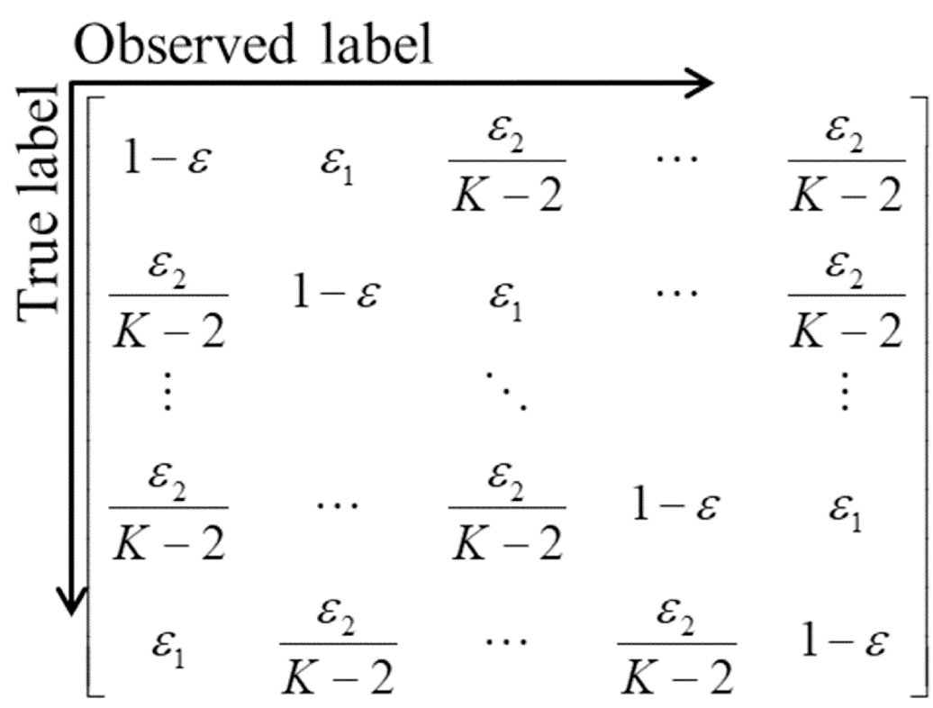
We used CIFAR-10 (Krizhevsky et al., 2009), CIFAR-100 (Krizhevsky et al., 2009), and Tiny-ImageNet (Tin, ), which are widely used benchmark datasets in the noisy label fields (Han et al., 2018c; Song et al., 2019; Yu et al., 2019; Kong et al., 2019; Arazo et al., 2019; Chen et al., 2019; Kim et al., 2019). CIFAR-10 and CIFAR-100 consist of $10$ and $100$ classes, respectively, of $32\,\times\,32$ color images. Each class is composed of subsets with $80$ million categorical images. The numbers of their training and test data are $50,000$ and $10,000$, respectively. Tiny-ImageNet, a subset of ImageNet, consists of $200$ classes. Its numbers of training and test data are $100,000$ and $10,000$, respectively. The experiment was conducted by resizing the images from $64\,\times\,64$ to $32\,\times\,32$. These benchmark datasets consist only of clean samples. Therefore, we artificially corrupted their labels using three commonly used types of noise transition matrices: pair flipping (Fig. 4a), symmetry flipping (Fig. 4b), and mixed flipping (Fig. 4c) (Tanaka et al., 2018; Han et al., 2018c; Song et al., 2019; Yu et al., 2019; Kong et al., 2019). From (Han et al., 2018c), pair flipping is a more general case compared to symmetry flipping in the real world. In addition, we conducted experiments based on various noise rates: $\varepsilon=\left\{10\%,20\%,30\%,40\%\right\}$ for pair flipping and $\varepsilon=\left\{0\%,20\%,40\%,60\%\right\}$ for symmetry flipping. Finally, we conducted experiments for mixed flipping with a noise rate 40% where the labels are corrupted by labels of a class as $\varepsilon_{1}=30\%$ and the other classes as $\varepsilon_{2}=10\%$ (Fig. 4c).

Thereafter, the ANIMAL-10N dataset (Song et al., 2019) and Clothing1M (Xiao et al., 2015), whose data are collected from the real world, were employed to examine the performance of Criteria_ALL. ANIMAL-10N dataset, whose labels were corrupted by human errors, consists of images from 10 animals of similar appearance. The numbers of its training and test data are $50,000$ and $5,000$, respectively, and its noise rate is $8\%$. Furthermore, an experiment was conducted with $64\,\times\,64$ color images without data augmentation or pre-processing. The Clothing1M dataset, which contains 1 million images of clothing, was obtained from online shopping websites with 14 classes. The labels were assigned by surrounding text of images provided by the sellers, and thus the dataset contains severe noisy labels. Its overall accuracy of the labels is $61.54\%$ (Xiao et al., 2015). The numbers of training and test data were $1,000,000$ and $100,000$, respectively.

B.3 System setup

To compare their performances, the experiments were conducted using DenseNet $\left(\mathrm{L}=25,\mathrm{k}=12\right)$ (Huang et al., 2017b) with a momentum optimizer $\left(\gamma=0.9\right)$. Moreover, we have set a batch size of $128$ and applied dropout (Srivastava et al., 2014) (dropout rate $=0.2$) and batch normalization (Ioffe & Szegedy, 2015). The learning was conducted for $100$ epochs with an initial learning rate of $0.1$ by reducing the rate by $0.2$ times at the $50$th and $75$th epochs. For the algorithms, the training was conducted without processing for noisy labels until $25$ epochs (warm-up threshold $=25$) for initial learning, similar to (Song et al., 2019). In Co-teaching, we set $\mathrm{T}_{k}=15$ and assumed that $\varepsilon$ is known (Han et al., 2018c; Song et al., 2019; Wang et al., 2019a; Yu et al., 2019). If $\varepsilon$ is unknown in advance, its value can be inferred from the validation set (Song et al., 2019; Liu & Tao, 2015; Yu et al., 2018). In SL and SL–Prop, we set the hyperparameters as $\alpha=1$ for all dataset, whereas $\beta$ is set depending on the dataset (CIFAR-10: 0.08, CIFAR-100: 0.3, Tiny-ImageNet: 0.3, ANIMAL-10N: 0.01, Clothing1M: 0.08). In SELFIE, we set the uncertainty threshold to $0.05$, history length to $15$, and restart to $2$ (totally three runs), as in (Song et al., 2019). In SELFIE–Prop, samples can be corrected precisely owing to the capability of Criteria_ALL that distinguishes clean and noisy samples regardless of noise type. Therefore, we set the hyperparameter tightly (uncertainty threshold $=0.005$ and history length $=25$) for SELFIE–Prop. Moreover, we set $\lambda$ to 1 by the experiments in Section B.7 and $\bm{q}$ is assumed to be uniform in the benchmark and real-world datasets.

B.4 Experimental result on symmetry flipping case

In the symmetry flipping case, because no dominant noisy samples were present, MentorNet–Prop should have exhibited similar performance as MentorNet, as indicated in Theorem 1 (Fig. 7).

B.5 Experimental result on a real-world dataset

Table 3: Best test error (%) in ANIMAL-10N (8% noise)

Algorithm	Default	Active Bias	Co-teaching	Co-teaching+	MentorNet	SL	SELFIE	MentorNet–Prop	SL–Prop	SELFIE–Prop
DenseNet (L=25, k=12)	17.9 $\pm$0.02	17.6 $\pm$0.17	17.5 $\pm$0.17	23.6 $\pm$0.20	18.0 $\pm$0.15	17.3 $\pm$0.05	17.0 $\pm$0.10	16.5 $\pm$0.19	16.3 $\pm$0.04	16.1 $\pm$0.13

We applied the algorithms on the ANIMAL-10N and Clothing1M to examine the effectiveness of Criteria_ALL in real-world datasets. From (Song et al., 2019), the ANIMAL-10N dataset was influenced by human errors during the image labeling process, because the classes consist of five pairs of “confusing” animals. The noise rate ($\varepsilon=8\%$) was estimated by cross-validation with grid search (Song et al., 2019). The experimental results indicate that the test error of MentorNet–Prop was $0.5\%$ lower than that of SELFIE, which exhibited the lowest test error among the conventional algorithms (Table 3). Furthermore, SL–Prop and SELFIE–Prop achieved a test error $1.0\%$ and $0.9\%$ lower than that of SL and SELFIE, respectively. Because the noise rate was small ($8\%$), the difference in performance was small. However, the experimental results indicate that Criteria_ALL is still effective.

Table 4: Test error (%) in Clothing1M

Algorithm	Default	VAT (Miyato et al., 2018)	F–correction (Patrini et al., 2017)	GCE (Zhang & Sabuncu, 2018)	LCCN (Yao et al., 2019)	DMI (Xu et al., 2019)	MentorNet	SL	MentorNet-Prop	SL-Prop
ResNet-50	31.06	30.43	29.17	30.91	28.37	27.54	30.70	29.40	27.44	26.98

Experiments for Clothing1M were conducted using pretrained ResNet-50 as (Xu et al., 2019). We fine-tuned the network for 10 epochs where the learning rate was $1.0\text{\times}{10}^{-6}$ for the first 5 epochs and $0.5\text{\times}{10}^{-6}$ in the next 5 epochs. Several methods in loss correction (Patrini et al., 2017; Xu et al., 2019; Miyato et al., 2018; Zhang & Sabuncu, 2018; Yao et al., 2019) were compared with the proposed method, and we used the results reported by (Xu et al., 2019). Experimental results indicate that our MentorNet–Prop had lower test errors than whole conventional algorithms (Table 4). When the loss of MentorNet is changed to the loss of SL (SL–Prop), we can achieve $0.46\%$ lower test error than MentorNet–Prop. Consequently, we can show that the Criteria_ALL is effective for real-world datasets.

B.6 Effect of update method for penalty label

It is important to estimate a penalty label accurately when Criteria_ALL is used. To increase the accuracy of the penalty label, we propose the temporal ensemble method (Section A.1.1; Algorithm 3). With regard to the update method, Algorithm 3 exhibited a lower test error than that of Algorithm 2 for pair and symmetry flipping (Table 5). Because the predictions were stored per iteration, diverse predictions were obtained, and thus the penalty label can be estimated stably using the ensemble effect. Furthermore, the difference between these two update methods was apparent for pair flipping because penalty label is significantly effective for that noise type.

Table 5: Best test error (%) of MentorNet–Prop depending on update methods for penalty label and considering noise rate of $40\%$

Dataset	Method	Pair flipping	Symmetry flipping
CIFAR-10	Algorithm 2	30.8	14.5
	Algorithm 3	12.2	14.4
CIFAR-100	Algorithm 2	42.9	39.4
	Algorithm 3	36.6	38.4
Tiny-ImageNet	Algorithm 2	73.0	62.1
	Algorithm 3	62.5	61.0

B.7 Experiments on the hyperparameter

Figure 8: Experiments on hyperparameter at noise rate $40\%$ in CIFAR-100.

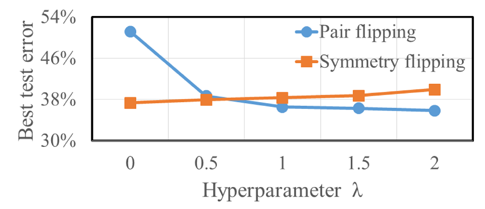
The Criteria_ALL exhibits only one hyperparameter $\lambda$ that adjusts the influence between Criteria_OL and Criteria_PL. To analyze the effect of $\lambda$, experiments were conducted with several values of $\lambda\,\left(=\left\{0.0,0.5,1.0,1.5,2.0\right\}\right)$, at a noise rate of $40\%$ in CIFAR-100 for both pair and symmetry flipping (Fig. 8). In pair flipping, the test error decreased steeply when $\lambda$ was lower than one owing to the high effectiveness of the penalty label. In symmetry flipping, the test error slightly increased with increasing $\lambda$, owing to the incorrect penalty label. Therefore, we empirically set $\lambda=1$ to consider the trade-off between pair and symmetry flipping.

B.8 Discussion

In this section, we discuss the effect of Criteria_OL, Criteria_PL, and Criteria_ALL on sample selection, and the difference between penalty label and noise transition matrix for pair and symmetry flipping cases.

B.8.1 Comparison of precisions of the criteria

(a)

(b)

Figure 9: Precision of Criteria_OL, Criteria_PL, and Criteria_ALL at noise rate $40\%$ in CIFAR-100; (a) pair flipping; (b) symmetry flipping.

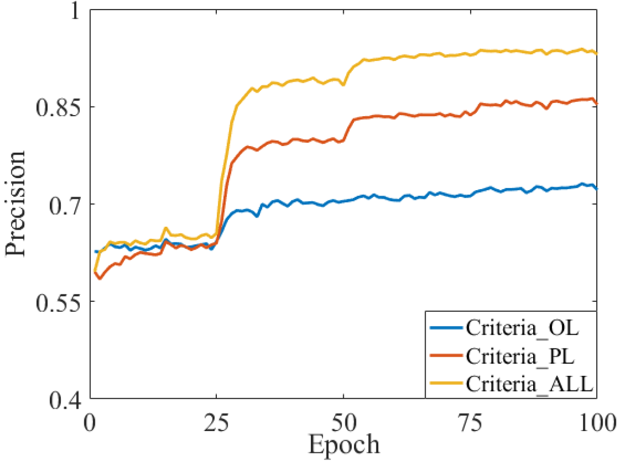
The precisions of Criteria_OL, Criteria_PL, and Criteria_ALL were compared to examine the performance in selecting clean samples for each epoch (Fig. 9). Each criteria was applied to MentorNet from the $25$th epoch (warm-up). In addition, the learning rate was reduced by $0.2$ times at the $50$th and $75$th epochs. In the pair flipping case, owing to the shared patterns of dominant noisy samples, severe memorization occurred. This results in a precision of approximately $70\%$ for Criteria_OL. In contrast, owing to the penalty applied to the dominant noisy samples, the precision of Criteria_PL was approximately $15\%$ higher than that of Criteria_OL. Furthermore, Criteria_ALL, which uses the two complementary criteria simultaneously, exhibited the highest precision (approximately $92\%$), because Criteria_OL and Criteria_PL evaluate samples through different patterns caused by observed label and penalty label.

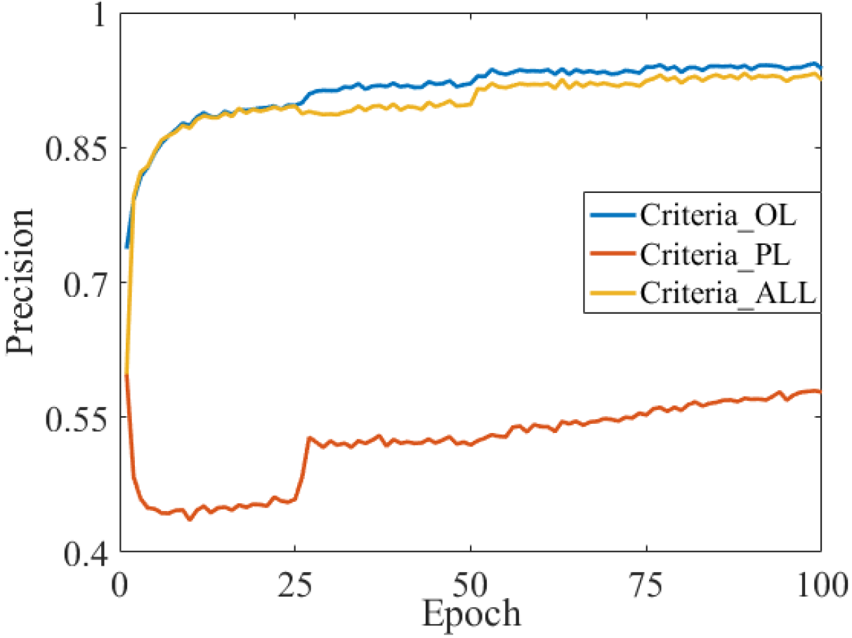
In symmetry flipping, because there were no dominant noisy samples, Criteria_OL exhibited a high precision (approximately $92\%$), whereas Criteria_PL did not affect the selection of clean samples (approximately $60\%$ precision). Initially, Criteria_ALL exhibited lower precision than Criteria_OL. However, as the training stage progressed, the accuracy of estimation of the penalty labels increased steadily, and the precision was similar to that of Criteria_OL.

B.8.2 Comparison between Criteria_ALL and noise transition matrix

Table 6: Best test error (%) of Default, loss correction with noise transition matrix (F–correction), and MentorNet–Prop with noise rate of $40\%$ in Tiny-ImageNet

Algorithm	Default	F–correction	MentorNet–Prop
Pair flipping	69.9	72.8	62.5
Symmetry flipping	64.7	75.3	61.0

The average-prediction confidence of each observed label (which is used to estimate the penalty label) can also be used to estimate the noise transition matrix. Therefore, the performance of the sample selection using Criteria_ALL (MentorNet–Prop) was compared with that of F–correction (Patrini et al., 2017), a representative method of loss correction with a noise transition matrix. In this case, the noise transition matrix was replaced by the average-prediction confidence used to estimate proposed penalty label in Criteria_PL. From (Han et al., 2018c; Song et al., 2019; Jiang et al., 2018), it is challenging to estimate the noise transition matrix when the number of classes is large. Consequently, the noise transition matrix, estimated by the average-prediction confidence of each observed label in Tiny-ImageNet ($200$ classes), was inaccurate. Furthermore, F–correction does not distinguish clean and noisy samples, unlike MentorNet–Prop. Therefore, in Table 6, F–correction achieved a test error even $2.9$–$10.6\%$ higher than that of the Default. In contrast, because in Criteria_ALL, only relative average-prediction confidence is needed to significantly penalize the dominant noisy samples unlike noise transition matrix, MentorNet–Prop exhibited remarkable performance regardless of the number of classes (Tables 1, 6).

Appendix C Special case: Symmetry flipping

If the label of a true class is corrupted by the labels of the other classes with the same noise rate (symmetry flipping), Criteria_PL should not affect the selection of clean samples because there are no dominant noisy samples and penalty label has same value. This property is stated in the following Theorem.

Theorem 1

Supposing that the noise type is symmetry flipping with ideal penalty label ($\mathit{\textit{{m}}^{k}=\frac{1}{K-1}}$), the order of samples with Criteria_ALL is identical to that with Criteria_OL as

$${\mathrm{ORDER}}_{\left({\mathbf{x}}_{i},{\hat{\mathbf{y}}}_{i}\right)\in{\mathcal{B}}}^{\mathrm{Descent}}\mathrm{Criteria\_ALL}\left({\mathbf{x}}_{i},{\hat{\mathbf{y}}}_{i},{\tilde{\mathbf{y}}}_{i};{\bm{\theta}}\right)={\mathrm{ORDER}}_{\left({\mathbf{x}}_{i},{\hat{\mathbf{y}}}_{i}\right)\in{\mathcal{B}}}^{\mathrm{Descent}}\mathrm{Criteria\_OL}\left({\mathbf{x}}_{i},{\hat{\mathbf{y}}}_{i};{\bm{\theta}}\right).$$

Proof.

$$\mathrm{Criteria\_ALL}\left({\mathbf{x}}_{i},{\hat{\mathbf{y}}}_{i},{\tilde{\mathbf{y}}}_{i};{\bm{\theta}}\right) = \sum_{j}{\hat{\mathbf{y}}}_{i}\left(j\right)P\left(\mathbf{y}=\mathbf{e}^{j}|{\mathbf{x}}_{i};\bm{\theta}\right)-\lambda\sum_{j}{\tilde{\mathbf{y}}}_{i}\left(j\right)P\left(\mathbf{y}=\mathbf{e}^{j}|{\mathbf{x}}_{i};\bm{\theta}\right)$$

$$= \sum_{j}{\mathbf{e}^{k}}\left(j\right)P\left(\mathbf{y}=\mathbf{e}^{j}|{\mathbf{x}}_{i};\bm{\theta}\right)-\lambda\sum_{j}{\mathbf{m}^{k}}\left(j\right)P\left(\mathbf{y}=\mathbf{e}^{j}|{\mathbf{x}}_{i};\bm{\theta}\right)\quad\left(\because{\hat{\mathbf{y}}}_{i}={\mathbf{e}^{k}},{\tilde{\mathbf{y}}}_{i}={\mathbf{m}^{k}}\right)$$

$$= \sum_{j=k}P\left(\mathbf{y}=\mathbf{e}^{j}|{\mathbf{x}}_{i};\bm{\theta}\right)-\frac{\lambda}{K-1}\sum_{j\neq k}P\left(\mathbf{y}=\mathbf{e}^{j}|{\mathbf{x}}_{i};\bm{\theta}\right)\quad$$

$$\left(\because\mathrm{In}\ \mathrm{ideal}\ \mathrm{case,}\ {\mathbf{m}^{k}}\left(j\right)=\frac{1}{K-1}\,\mathrm{for}\;j\neq k\right)$$

$$= \sum_{j=k}P\left(\mathbf{y}=\mathbf{e}^{j}|{\mathbf{x}}_{i};\bm{\theta}\right)-\frac{\lambda}{K-1}\left(1-\sum_{j=k}P\left(\mathbf{y}=\mathbf{e}^{j}|{\mathbf{x}}_{i};\bm{\theta}\right)\right)$$

$$\left(\because\sum_{j}P\left(\mathbf{y}=\mathbf{e}^{j}|{\mathbf{x}}_{i};\bm{\theta}\right)=1\right)$$

$$= \left(1+\frac{\lambda}{K-1}\right)\sum_{j=k}P\left(\mathbf{y}=\mathbf{e}^{j}|{\mathbf{x}}_{i};\bm{\theta}\right)-\frac{\lambda}{K-1}$$

$$= \left(1+\frac{\lambda}{K-1}\right)\sum_{j}{\hat{\mathbf{y}}}_{i}\left(j\right)P\left(\mathbf{y}=\mathbf{e}^{j}|{\mathbf{x}}_{i};\bm{\theta}\right)-\frac{\lambda}{K-1}$$

$$= \left(1+\frac{\lambda}{K-1}\right)\mathrm{Criteria\_OL}\left({\mathbf{x}}_{i},{\hat{\mathbf{y}}}_{i};{\bm{\theta}}\right)-\frac{\lambda}{K-1}.$$

Because the scaling and bias do not alter the order, the order of samples with both the criteria is identical.  $\square$

References

- (1) https://tiny-imagenet.herokuapp.com/.
- Arazo et al. (2019) Arazo, E., Ortego, D., Albert, P., O’Connor, N., and McGuinness, K. Unsupervised label noise modeling and loss correction. In International Conference on Machine Learning, pp. 312–321. PMLR, 2019.
- Arpit et al. (2017) Arpit, D., Jastrzebski, S., Ballas, N., Krueger, D., Bengio, E., Kanwal, M. S., Maharaj, T., Fischer, A., Courville, A., Bengio, Y., et al. A closer look at memorization in deep networks. In International Conference on Machine Learning, pp. 233–242. PMLR, 2017.
- Cha & Cho (2012) Cha, Y. and Cho, J. Social-network analysis using topic models. In Proceedings of the 35th international ACM SIGIR conference on Research and development in information retrieval, pp. 565–574, 2012.
- Chang et al. (2017) Chang, H.-S., Learned-Miller, E., and McCallum, A. Active bias: Training more accurate neural networks by emphasizing high variance samples. arXiv preprint arXiv:1704.07433, 2017.
- Chen et al. (2019) Chen, P., Liao, B. B., Chen, G., and Zhang, S. Understanding and utilizing deep neural networks trained with noisy labels. In International Conference on Machine Learning, pp. 1062–1070. PMLR, 2019.
- Goldberger & Ben-Reuven (2016) Goldberger, J. and Ben-Reuven, E. Training deep neural-networks using a noise adaptation layer. 2016.
- Han et al. (2018a) Han, B., Pan, Y., and Tsang, I. W. Robust plackett–luce model for k-ary crowdsourced preferences. Machine Learning, 107(4):675–702, 2018a.
- Han et al. (2018b) Han, B., Yao, J., Niu, G., Zhou, M., Tsang, I., Zhang, Y., and Sugiyama, M. Masking: A new perspective of noisy supervision. arXiv preprint arXiv:1805.08193, 2018b.
- Han et al. (2018c) Han, B., Yao, Q., Yu, X., Niu, G., Xu, M., Hu, W., Tsang, I., and Sugiyama, M. Co-teaching: Robust training of deep neural networks with extremely noisy labels. arXiv preprint arXiv:1804.06872, 2018c.
- Hendrycks et al. (2018) Hendrycks, D., Mazeika, M., Wilson, D., and Gimpel, K. Using trusted data to train deep networks on labels corrupted by severe noise. arXiv preprint arXiv:1802.05300, 2018.
- Huang et al. (2017a) Huang, G., Li, Y., Pleiss, G., Liu, Z., Hopcroft, J. E., and Weinberger, K. Q. Snapshot ensembles: Train 1, get m for free. arXiv preprint arXiv:1704.00109, 2017a.
- Huang et al. (2017b) Huang, G., Liu, Z., Van Der Maaten, L., and Weinberger, K. Q. Densely connected convolutional networks. In Proceedings of the IEEE conference on computer vision and pattern recognition, pp. 4700–4708, 2017b.
- Ioffe & Szegedy (2015) Ioffe, S. and Szegedy, C. Batch normalization: Accelerating deep network training by reducing internal covariate shift. In International conference on machine learning, pp. 448–456. PMLR, 2015.
- Jiang et al. (2018) Jiang, L., Zhou, Z., Leung, T., Li, L.-J., and Fei-Fei, L. Mentornet: Learning data-driven curriculum for very deep neural networks on corrupted labels. In International Conference on Machine Learning, pp. 2304–2313. PMLR, 2018.
- Kim et al. (2019) Kim, Y., Yim, J., Yun, J., and Kim, J. Nlnl: Negative learning for noisy labels. In Proceedings of the IEEE/CVF International Conference on Computer Vision, pp. 101–110, 2019.
- Kong et al. (2019) Kong, K., Lee, J., Kwak, Y., Kang, M., Kim, S. G., and Song, W.-J. Recycling: Semi-supervised learning with noisy labels in deep neural networks. IEEE Access, 7:66998–67005, 2019.
- Krizhevsky et al. (2009) Krizhevsky, A., Hinton, G., et al. Learning multiple layers of features from tiny images. 2009.
- Laine & Aila (2016) Laine, S. and Aila, T. Temporal ensembling for semi-supervised learning. arXiv preprint arXiv:1610.02242, 2016.
- Liu & Tao (2015) Liu, T. and Tao, D. Classification with noisy labels by importance reweighting. IEEE Transactions on pattern analysis and machine intelligence, 38(3):447–461, 2015.
- Liu et al. (2011) Liu, W., Jiang, Y.-G., Luo, J., and Chang, S.-F. Noise resistant graph ranking for improved web image search. In CVPR 2011, pp. 849–856. IEEE, 2011.
- Malach & Shalev-Shwartz (2017) Malach, E. and Shalev-Shwartz, S. Decoupling” when to update” from” how to update”. arXiv preprint arXiv:1706.02613, 2017.
- Miyato et al. (2018) Miyato, T., Maeda, S.-i., Koyama, M., and Ishii, S. Virtual adversarial training: a regularization method for supervised and semi-supervised learning. IEEE transactions on pattern analysis and machine intelligence, 41(8):1979–1993, 2018.
- Patrini et al. (2017) Patrini, G., Rozza, A., Krishna Menon, A., Nock, R., and Qu, L. Making deep neural networks robust to label noise: A loss correction approach. In Proceedings of the IEEE Conference on Computer Vision and Pattern Recognition, pp. 1944–1952, 2017.
- Reed et al. (2014) Reed, S., Lee, H., Anguelov, D., Szegedy, C., Erhan, D., and Rabinovich, A. Training deep neural networks on noisy labels with bootstrapping. arXiv preprint arXiv:1412.6596, 2014.
- Ren et al. (2018) Ren, M., Zeng, W., Yang, B., and Urtasun, R. Learning to reweight examples for robust deep learning. In International Conference on Machine Learning, pp. 4334–4343. PMLR, 2018.
- Shen & Sanghavi (2019) Shen, Y. and Sanghavi, S. Learning with bad training data via iterative trimmed loss minimization. In International Conference on Machine Learning, pp. 5739–5748. PMLR, 2019.
- Song et al. (2019) Song, H., Kim, M., and Lee, J.-G. Selfie: Refurbishing unclean samples for robust deep learning. In International Conference on Machine Learning, pp. 5907–5915. PMLR, 2019.
- Srivastava et al. (2014) Srivastava, N., Hinton, G., Krizhevsky, A., Sutskever, I., and Salakhutdinov, R. Dropout: a simple way to prevent neural networks from overfitting. The journal of machine learning research, 15(1):1929–1958, 2014.
- Tanaka et al. (2018) Tanaka, D., Ikami, D., Yamasaki, T., and Aizawa, K. Joint optimization framework for learning with noisy labels. In Proceedings of the IEEE Conference on Computer Vision and Pattern Recognition, pp. 5552–5560, 2018.
- Wang et al. (2019a) Wang, X., Wang, S., Wang, J., Shi, H., and Mei, T. Co-mining: Deep face recognition with noisy labels. In Proceedings of the IEEE/CVF International Conference on Computer Vision, pp. 9358–9367, 2019a.
- Wang et al. (2019b) Wang, Y., Ma, X., Chen, Z., Luo, Y., Yi, J., and Bailey, J. Symmetric cross entropy for robust learning with noisy labels. In Proceedings of the IEEE/CVF International Conference on Computer Vision, pp. 322–330, 2019b.
- Welinder et al. (2010) Welinder, P., Branson, S., Perona, P., and Belongie, S. The multidimensional wisdom of crowds. Advances in neural information processing systems, 23:2424–2432, 2010.
- Xiao et al. (2015) Xiao, T., Xia, T., Yang, Y., Huang, C., and Wang, X. Learning from massive noisy labeled data for image classification. In Proceedings of the IEEE conference on computer vision and pattern recognition, pp. 2691–2699, 2015.
- Xu et al. (2019) Xu, Y., Cao, P., Kong, Y., and Wang, Y. L_dmi: A novel information-theoretic loss function for training deep nets robust to label noise. In NeurIPS, pp. 6222–6233, 2019.
- Yan et al. (2014) Yan, Y., Rosales, R., Fung, G., Subramanian, R., and Dy, J. Learning from multiple annotators with varying expertise. Machine learning, 95(3):291–327, 2014.
- Yao et al. (2019) Yao, J., Wu, H., Zhang, Y., Tsang, I. W., and Sun, J. Safeguarded dynamic label regression for noisy supervision. In Proceedings of the AAAI Conference on Artificial Intelligence, volume 33, pp. 9103–9110, 2019.
- Yu et al. (2018) Yu, X., Liu, T., Gong, M., Batmanghelich, K., and Tao, D. An efficient and provable approach for mixture proportion estimation using linear independence assumption. In Proceedings of the IEEE Conference on Computer Vision and Pattern Recognition, pp. 4480–4489, 2018.
- Yu et al. (2019) Yu, X., Han, B., Yao, J., Niu, G., Tsang, I., and Sugiyama, M. How does disagreement help generalization against label corruption? In International Conference on Machine Learning, pp. 7164–7173. PMLR, 2019.
- Zhang et al. (2016) Zhang, C., Bengio, S., Hardt, M., Recht, B., and Vinyals, O. Understanding deep learning requires rethinking generalization. arXiv preprint arXiv:1611.03530, 2016.
- Zhang & Sabuncu (2018) Zhang, Z. and Sabuncu, M. R. Generalized cross entropy loss for training deep neural networks with noisy labels. arXiv preprint arXiv:1805.07836, 2018.