1 Introduction

We consider a class of semi-parametric dynamic models with strong white noise error terms. This class includes the standard Vector Autoregressive (VAR) model, the nonfundamental structural VAR, the mixed causal-noncausal models, as well as nonlinear dynamic models, such as the ARCH-M model. The assumption on the error term is used to define the Generalized Covariance (GCov) estimator of the parameter of interest by minimizing a residual-based multivariate portmanteau statistic. The GCov estimator is introduced as a semi-parametric alternative to the GMM estimator. This estimation approach can be applied to multivariate or univariate models. In the latter case, the objective function to be minimized can be computed from the univariate series, or from several (nonlinear) transformations of the univariate series obtained, for example, by discretizing the state space. We show that the GCov estimator is consistent and asymptotically normally distributed. The expression of the asymptotic variance of the GCov estimator is considerably simplified due to the underlying standardization of the criterion to be minimized. This allows us to establish the semi-parametric efficiency of the GCov estimator. For testing the white noise hypothesis, we consider the residual-based multivariate portmanteau statistic. We show that this statistic follows asymptotically a chi-square distribution with the degrees of freedom adjusted for the number of identifiable parameters. This extends this well-known result, commonly used for linear dynamic VAR-type models, to a nonlinear dynamic framework.

The following notation is used. For any $m\times n$ matrix $A$ whose $j$th column is $a_{j}(j=1,...,n)$, $vec(A)$ will denote the column vector of dimension $mn$ defined as:

$$vec(A)=(a_{1}^{\prime}...,a_{j}^{\prime},...,a_{n}^{\prime})^{\prime},$$

where the prime denotes transposition. For any two matrices $A\equiv(a_{ij})$ and $B$, the Kronecker product $(A\otimes B)$ is the block matrix having $a_{ij}B$ for its $(i,j)$th block.

The paper is organized as follows. Section 2 recalls the interpretation and asymptotic distribution of the multivariate portmanteau statistic. Section 3 defines the GCov estimator and provides examples of semi-parametric models, which can be estimated by the GCov estimator. We also discuss the identifiability of the parameter of interest. Section 4 presents the results on the consistency and asymptotic normality of the GCov estimator. The residual-based multivariate portmanteau statistic and its distribution are examined in Section 5. The finite-sample performance of the GCov estimator is illustrated in Section 6 in a simulation study of ARCH-type models and mixed causal-noncausal models. The GCov estimator is also applied to the dynamic model of cryptocurrency prices. Section 7 concludes. Proofs and asymptotic expansions are gathered in Appendices 1 to 3.

2 The Weak White Noise Hypothesis

Let us consider a univariate stationary time series $(y_{t})$ with finite fourth-order moments. The test of the Weak White Noise hypothesis $H_{0}=\{\gamma(h)=0,h=1,....,H\}$, with $\gamma(h)=Cov(y_{t},y_{t-h})$ is commonly based on the test statistic:

$$\xi(H)=T\sum_{h=1}^{H}\hat{\rho}(h)^{2}=T\sum_{h=1}^{H}\frac{\hat{\gamma}(h)^{2}}{\hat{\gamma}(0)^{2}},$$ (2.1)

where $\hat{\gamma}(h)$ and $\hat{\rho}(h)$ are the sample autocovariance and autocorrelation of order $h$, respectively.

This statistic asymptotically follows a chi-square distribution $\chi^{2}(H)$ with $H$ degrees of freedom [see, Box, Pierce (1970)]. The aim of this Section is to review the analogue of this statistic for stationary time series of higher dimension.

Let us now consider a strictly stationary time series $(Y_{t})$ of dimension $K$ with finite fourth-order moments. The null hypothesis is now $H_{0}=\{\Gamma(h)=0,h=1,....,H\}$, where $\Gamma(h)=cov(y_{t},y_{t-h})$ is the autocovariance of order $h$. The sample autocovariance is denoted by $\hat{\Gamma}(h)$ . The multivariate analogue of (2.1) is:

$$\xi(H)=T\sum_{h=1}^{H}Tr[\hat{R}^{2}(h)],$$ (2.2)

where $\hat{R}^{2}(h)$ is the sample analogue of the multivariate R-square defined by:

$$R^{2}(h)=\Gamma(h)\Gamma(0)^{-1}\Gamma(h)^{\prime}\Gamma(0)^{-1}.$$ (2.3)

Since

$$\hat{R}^{2}(h)=\hat{\Gamma}(0)^{1/2}[\hat{\Gamma}(0)^{-1/2}\hat{\Gamma}(h)\hat{\Gamma}(0)^{-1}\hat{\Gamma}(h)^{\prime}\hat{\Gamma}(0)^{-1/2}]\hat{\Gamma}(0)^{-1/2},$$ (2.4)

this matrix is equivalent up to a change of basis of the matrix within brackets, which is symmetric, positive-definite. Therefore, it is diagonalisable, with a trace equal to the sum of its eigenvalues, which are the squares of the canonical correlations between $Y_{t}$ and $Y_{t-h}$, denoted by $\hat{\rho}_{j}^{2}(h),j=1,....,K$ [Hotelling (1936)]. Therefore:

$$\xi(H)=T\sum_{h=1}^{H}Tr[\hat{\Gamma}(h)\hat{\Gamma}(0)^{-1}\hat{\Gamma}(h)^{\prime}\hat{\Gamma}(0)^{-1}]=T\sum_{h=1}^{H}[\sum_{j=1}^{K}\hat{\rho}_{j}(h)^{2}].$$ (2.5)

Under the null hypothesis of Weak White Noise, this statistic follows asymptotically a chi-square distribution $\chi^{2}(KH)$ [see, e.g. Chitturi (1974), Robinson (1973), Anderson (1999), Section 7, Anderson (2002), Section 5].

In the special case when $\Gamma(0)$ is a diagonal matrix, formula (2.5) can be equivalently written as the sum of elements $\hat{\rho}_{ij}^{2}(h),i,j=1,....,K$, where $\hat{\rho}_{j}(h)$ are the elements of matrices of multivariate autocorrelations $\hat{D}^{-1/2}\Gamma(h)\hat{D}^{-1/2}$, where $\hat{D}$ is a diagonal matrix of variances of the component series .

Remark 1: In the literature, there exist alternative test statistics that are asymptotically equivalent to the test statistic $\xi(H)$ under the null. For example, we can consider the Seemingly Unrelated Regression (SUR) model:

$$Y_{t}=\alpha+B_{1}Y_{t-1}+\cdots+B_{H}Y_{t-H}+u_{t},$$ (2.6)

and introduce the statistic:

$$\tilde{\xi}(H)=T\;Tr[\hat{\Gamma}^{*}(1)\hat{\Gamma}^{*}(0)^{-1}\hat{\Gamma}^{*}(1)^{\prime}\hat{\Gamma}^{*}(0)^{-1}],$$ (2.7)

where $\Gamma^{*}(1)=Cov(Y_{t},\underline{Y_{t-1}}),\Gamma^{*}(0)=V(\underline{Y_{t-1}})$ and $\underline{Y_{t-1}}=(Y_{t-1}^{\prime},....,Y^{\prime}_{t-H})^{\prime}$.

Under the null, the explanatory variables in (2.6) are (asymptotically) uncorrelated, as the autoregressive coefficients $\hat{\Gamma}(h)\hat{\Gamma(0)}^{-1}$ [see, Mann, Wald (1943), Chitturi (1974), eq. (2.9)], which explains the possibility to replace the canonical correlation analysis of dimension $KH$ by $H$ canonical correlations of dimension $K$ only. We derive directly the asymptotic distribution of this statistic under the null in Appendix 1.

3 GCov Estimator

First, we introduce a class of semi-parametric multivariate nonlinear dynamic models with independent, identically distributed (i.i.d.) errors. This i.i.d. assumption is used to construct parameter estimators by minimizing the test statistic $L_{T}(\theta)=\xi(H;\theta)$, corresponding to the errors and the parameter value. The maximizer of $L_{T}(\theta)$ is defined as the Generalized Covariance (GCov) estimator. Next, the asymptotic properties of the GCov estimator are derived.

3.1 Semi-Parametric Model

Let us consider a semi-parametric model satisfying dynamic equations of the type:

$$g(\underline{Y_{t}};\theta)=u_{t},$$ (3.1)

where $g$ is a known function, $(u_{t})$ is a strong stationary white noise, and $\theta$ an unknown parameter. We assume that the model is well-specified with $\theta_{0}$ the true value of the parameter $\theta$. Such nonlinear structural VAR models are common in the literature, as shown in the examples below.

While the weak white noise assumption can be sufficient to define the GCov estimator and some of its asymptotic properties, the i.i.d. assumption is needed when various transformations of the series are considered and to discuss the parametric versus semi-parametric efficiency. It is also useful for the analysis of structural implementations of the models from nonlinear impulse responses [see e.g. Gourieroux, Monfort, Renne (2020), Sims(2021)]. In addition, it is commonly used in the recent literature on portmanteau tests [see e.g. Hoga(2021), Section 2].

Example 1: ARCH-M Model [Engle, Lillien, Robbins (1987)]

The model is:

$$y_{t}=m(y_{t-1};\theta_{1})+\theta_{3}\sigma(y_{t-1};\theta_{2})+\sigma(y_{t-1};\theta_{2})u_{t}.$$

It extends the standard ARCH-M model by allowing for nonlinear drift and volatility functions. We have:

$$g(\underline{y_{t}};\theta)=\frac{y_{t}-m(y_{t-1};\theta_{1})-\theta_{3}\sigma(y_{t-1};\theta_{2})}{\sigma(y_{t-1};\theta_{2})}.$$

Example 2: (Causal) VAR Model

The multivariate VAR(p) process is defined by:

$$Y_{t}=\Phi_{1}Y_{t-1}+\cdots+\Phi_{p}Y_{t-p}+u_{t},$$

where $\theta=[vec\Phi_{1}^{\prime},...,vec\Phi_{p}^{\prime}]^{\prime}.$

We assume that the roots of the characteristic equation $det(Id-\Phi_{1}\lambda-\cdots-\Phi_{p}\lambda^{p})=0$ are of modulus strictly larger than one. Then, there exists a unique (strictly) stationary solution $(Y_{t})$ with a causal $MA(\infty)$ representation. In this case we have:

$$g_{t}(Y,\theta)=Y_{t}-\Phi_{1}Y_{t-1}-\cdots\Phi_{p}Y_{t-p}.$$

The (causal) VAR model has been widely analyzed in the literature on residual-based portmanteau test [see e.g. Hosking (1980), Li, McLeod (1981)].

In the VAR specification parameters $\Phi_{1},...,\Phi_{p}$ can be constrained. This includes in particular:

i) The VAR(1) model with reduced rank for $\Phi_{1}$ [see, Velu et al. (1986), Ahn, Reinsel (1988), Engle, Kozicki (1993), Reinsel, Velu (1998), Anderson (2002), Lam, Yao (2012)].

ii) The VAR(p) model with common canonical directions at all lags [see Kettenring (1971), Neuenschwander, Flury ( 1995)].

iii) The VAR(p) processes with subprocesses assumed independent [see, e.g. Haugh (1976), El Himdi, Roy (1997), Duchesne, Roy (2003), Yata, Aoshima(2016), Jin, Matteson (2018)].

iv) The VAR(p) model with causality restrictions [see e.g. Boudjellaba et al. (1994)].

v) The VAR(p) model with a Kronecker structure [Niu et al. (2020)].

and all structural VAR models.

Example 3: Causal-Noncausal MAR(r,s) Model

A multivariate $MAR(r,s)$ process [see e.g. Gourieroux, Jasiak (2017)] with mixed causal and noncausal autoregressive dynamics is:

$$\Phi(L)\Psi(L^{-1})y_{t}=u_{t},$$

where the autoregressive polynomials $\Phi(L)$ and $\Psi(L^{-1})$ are of orders $r$ and $s$, respectively. The determinants of the autoregressive polynomials have roots outside the unit circle . The error $u_{t}$ is a non-Gaussian strong white noise process with finite first fourth moments. Then, vector $\theta$ includes all the autoregressive matrix coefficients and function g is:

$$g_{t}(y,\theta)=\Phi(L)\Psi(L^{-1})y_{t},\;\mbox{or}\;\;g(Y_{t};\theta)=\Phi(L)\Psi(L^{-1})L^{s}Y_{t},$$

where $Y_{t}=y_{t+s}$. In particular, for the univariate MAR(1,1) process, with $r=s=1$:

$$(1-\phi L)(1-\psi L^{-1})y_{t}=u_{t},$$

where $|\phi|<1$, $|\psi|<1$, the function $g$ is easily written as:

$$g(\underline{Y_{t}},\theta)=g(y_{t},y_{t+1},y_{t-1})=Y_{t-1}-\phi\psi-\phi Y_{t-2}-\psi Y_{t},$$

with $Y_{t}=y_{t+1}$.

The dependence of function $g$ on the past, present and future values of the observed process concerns also the application to SVAR models with nonfundamental features.

Example 4: Noncausal VAR Model

The multivariate noncausal VAR(p) process is defined by:

$$Y_{t}=\Phi_{1}Y_{t-1}+\cdots+\Phi_{p}Y_{t-p}+u_{t},$$

where $\theta=[vec\Phi_{1}^{\prime},...,vec\Phi_{p}^{\prime}]^{\prime}$ and the error $u_{t}$ is a multivariate non-Gaussian strong white noise process with finite first fourth moments.

We assume that the roots of the characteristic equation $det(Id-\Phi_{1}\lambda-\cdots\Phi_{p}\lambda^{p})=0$ are of modulus either strictly larger, or smaller than one. Then, there exists a unique (strictly) stationary solution $(Y_{t})$ with a two-sided $MA(\infty)$ representation:

$$g_{t}(Y,\theta)=Y_{t}-\Phi_{1}Y_{t-1}-\cdots-\Phi_{p}Y_{t-p}.$$

The non-causal VAR(p) model has been studied in Gourieroux, Jasiak (2017) and Davis, Song (2020).

Example 5: Stacking Nonlinear Transformations of $u_{t}$

From system (3.1), we can build systems of higher dimensions by considering nonlinear transformations of $u_{t}$. Let us introduce $J$ nonlinear transformations $a_{1},...,a_{J}$. Then we have:

$$a_{j}[g(\underline{y_{t}};\theta)] = a_{j}(u_{t}),\;j=1,...J,$$ (3.2)

$$\iff a[g(\underline{y_{t}};\theta)]=a(u_{t})=v_{t},$$

where the transformed process $(v_{t})$ is also a strong white noise.

For example, the financial returns $y_{t}$ can be stacked together with their squares: $Y_{t}=(y_{t},y_{t}^{2})$ [see e.g. Wooldridge (1991), Li, Mak (1994), Ling, Li (1997), Section 4], or with their absolute values $(Y_{t}=y_{t},|y_{t}|)$ [see Pena, Rodriguez (2006)], or return signs and squares $Y_{t}=(signy_{t},y_{t}^{2})$ can be stacked to separate their dynamic volatility from the bid-ask bounce effect.

3.2 The Estimator

When $(u_{t})$ is a strong white noise with finite moments up to order 4, $(u_{t})$ is also a weak white noise. We define the GCov estimator of $\theta$ in model (3.1) by considering:

$$\hat{\theta}_{T}(H)=Argmin_{\theta}\sum_{h=1}^{H}Tr[\hat{R}^{2}(h,\theta)],$$ (3.3)

where

$$\hat{R}^{2}(h,\theta)=\hat{\Gamma}(h;\theta)\hat{\Gamma}(0,\theta)^{-1}\hat{\Gamma}(h;\theta)^{\prime}\hat{\Gamma}(0;\theta)^{-1},$$ (3.4)

and $\hat{\Gamma}(h;\theta)$ is the sample covariance between $g(\underline{Y_{t}};\theta)$ and $g(\underline{Y_{t-h}};\theta)$.

Except for special cases such as the causal VAR model, where the GCov estimates of the $\Phi_{j}$ are equivalent to the OLS estimates, the GCov estimator has no closed-form expression.

Remark 2: Let us consider $H=1$ and assume the parameter $\theta$ such that $dim\theta=K^{2}$. This is the just identified case, when $\hat{\theta}_{T}$ is the solution of:

$$Tr\,\hat{R}^{2}(1;\hat{\theta}_{T})=0\iff\hat{R}^{2}(1;\hat{\theta}_{T})=0\iff\hat{\Gamma}(1;\hat{\theta}_{T})=0.$$

Thus, the GCov estimator is the analogue of a moment estimator based on centered cross-moments instead of uncentered cross-moments used in standard GMM.

Remark 3: If $(u_{t})$ has no fourth-order moment, the initial model (3.1) can be replaced by the transformed model (3.2), whenever the transformed errors $a_{j}(u_{t})$ have such moments. Then the GCov estimator depends on $H$ and transformation $a$.

Example 6: Discretization of the State Space

Let us consider a strictly stationary process $(y_{t})$ and a discretization defined by a partition of the state space: $A_{k},\;k=1,...,K+1$. We introduce the indicator functions $Y_{k,t},\;k=1,...,K+1$, such that $Y_{kt}=1$, if $y_{t}\in A_{k}$, and $Y_{kt}=0$, otherwise. Then, the transformed variables $Y_{k,t}$ have moments of any order, even if the moments of $(y_{t})$ do not exist. Since $\sum_{k=1}^{K+1}Y_{k,t}=1,\;\forall t$, we just consider the $K$ first components to define $Y_{t}$. Let us denote by $p$ the K-dimensional vector with components $p_{k}=P[y_{t}\in A_{k}]$ and $P(h)$ the $K\times K$ matrix with elements $p_{kl}(h)=P[y_{t}\in A_{k},y_{t-h}\in A_{l}]$. We have:

$$\Gamma(h)=P(h)-pp^{\prime},\;\Gamma(0)=diagp-pp^{\prime}\;\mbox{and}\;\Gamma(0)^{-1}=diag(P^{-1})-\frac{ee^{\prime}}{1-e^{\prime}p},$$

where $e$ is the $K$-dimensional vector with unitary components. Then, it is easy to check that:

$$\sum_{h=1}^{H}Tr\,R^{2}(h)=\sum_{h=1}^{H}[\sum_{k=1}^{K+1}\sum_{l=1}^{K+1}\frac{(p_{kl}(h)-p_{k}p_{l})^{2}}{p_{k}p_{l}}]=\sum_{h=1}^{H}\chi^{*2}(h),$$

where $\chi^{*2}(h)$ is the chi-square measure of (in)dependence between $Y_{t}$ and $Y_{t-h}$. Thus, the GCov estimator minimizes a measure of pairwise (in)dependence.

4 Asymptotic Properties of the GCov Estimator

Let the objective function be denoted by $L_{T}(\theta)=\sum_{h=1}^{H}Tr\,\hat{R}^{2}(h;\theta)$. We provide below the asymptotic properties of the GCov estimator. The proof of these properties are given in Appendix 2.

4.1 Consistency and Identification

Under the strict stationarity of process $(Y_{t})$ and the existence of the second-order moments of $g(\underline{Y_{t}},\theta)$, the sample autocovariances $\hat{\Gamma}(h;\theta)$ tend to their theoretical counterparts $\Gamma(h;\theta)$ and, if $\Gamma(0;\theta)$ is invertible for $\theta\in\Theta$, then $L_{T}(\theta)$ tends to:

$$L_{\infty}(\theta)=\sum_{h=1}^{H}Tr\,[R^{2}(h;\theta)].$$ (4.1)

If model (3.1) is well-specified, we have $L_{\infty}(\theta_{0})=0$ and then the true value is the solution, which minimizes $\theta_{0}=Argmin_{\theta}L_{\infty}(\theta)$. By applying the standard Jennrich’s argument [Jennrich (1969), Andrews (1987)], we get the consistency of the GCov estimator under an identification condition.

Proposition 1: If $\theta=\theta_{0}$ is the unique solution of the minimization of the limiting objective function $L_{\infty}(\theta)$, then the GCov estimator $\hat{\theta}_{T}$ is consistent.

The uniqueness condition of the solution is an identification condition. It implies that some parameters might not be consistently approximated by a GCov estimator.

Example 6: Drift and Scale Parameters

The model (3.1) may include drift and scale parameters. In such a case:

$$g(\underline{Y_{t}};\theta)=C(\tilde{g}(\underline{Y_{t}};\alpha)-m),$$

with $\theta=(\alpha,m,C)$. Since $Tr\,R^{2}$ is invariant with respect to affine transformations, $m$ and $C$ are not identifiable. Then the GCov approach has to be applied to $\tilde{g}(Y_{t};\alpha)$ and parameter $\alpha$, corresponding to the identification restriction $m=0,C=Id$.

Example 7: Box-Cox transformation

The lack of identification can also arise in nonlinear transformations. For example, let us consider the model:

$$Y_{t}(\lambda)=\frac{Y_{t}^{\lambda}-1}{\lambda}=u_{t},$$ (4.2)

where the Box-Cox transform is applied to $Y_{t}$, provided that it is positive. It is equivalent to assume that the $Y_{t}$’s are i.i.d. or that the $Y_{t}(\lambda)$’s are i.i.d., then parameter $\lambda$ is not identifiable by the GCov approach.

Remark 4: The lack of identification of $\lambda$ can be explained by considering the analogue Quasi Maximum Likelihood (QML) approach. Let us consider model (4.2) with autoregressive errors:

$$u_{t}=m+\Phi(u_{t-1}-m)+C\epsilon_{t},$$

where $(\epsilon_{t})$ are i.i.d. $N(0,Id)$. The Gaussian log-likelihood has two components: the first component corresponds to the log-Jacobian of the nonlinear Box-Cox transform and the second component is the residual one. When this Gaussian log-likelihood is concentrated in $m,\Phi$ and $C$, the second component is close to $T\,Tr\,\hat{R}^{2}(1;\lambda)$ (when $\Phi=0$). In contrast to the GCov approach, a Gaussian QML approach identifies $\lambda$, since it accounts for the nonlinear Box-Cox transform through the log-Jacobian component.

If the functions $\Gamma(h;\theta),h=1,...,H$ are differentiable with respect to $\theta$ and $\theta_{0}$ is in the interior of the parameter set $\Theta$, the GCov estimator satisfies the first-order conditions (FOC):

$$\frac{\partial L_{T}(\hat{\theta}_{T})}{\partial\theta}=0\iff\sum_{k=1}^{K}\frac{\partial\,Tr\,\hat{R}^{2}(h;\hat{\theta}_{T})^{2}}{\partial\theta}=0.$$ (4.3)

Appendix A.2.1. provides the expressions of the derivatives. We have:

$$\frac{\partial\,Tr\,\hat{R}^{2}(h;\hat{\theta}_{T})}{\partial\theta_{j}} = 2\,Tr\,[\hat{\Gamma}(0;\hat{\theta}_{T})^{-1}\hat{\Gamma}(h;\hat{\theta}_{T})^{\prime}\hat{\Gamma}(0;\hat{\theta}_{T})^{-1}\frac{\partial\hat{\Gamma}(h;\hat{\theta}_{T})}{\partial\theta_{j}}$$ (4.4)

$$- Tr\,\{[\hat{\tilde{R}}^{2}(h;\hat{\theta}_{T})\hat{\Gamma}(0;\hat{\theta}_{T})^{-1}+\hat{\Gamma}(0;\hat{\theta}_{T})^{-1}\hat{R}^{2}(h;\hat{\theta}_{T})]\frac{\partial\hat{\Gamma}(0;\hat{\theta}_{T})}{\partial\theta_{j}}\},$$

for $j=1,...,J=dim\theta$.

Remark 5: When $K=1$, the coefficient of determination is a scalar $R^{2}(h;\theta)=\rho^{2}(h;\theta)$ and the FOC become:

$$\sum_{h=1}^{H}[\hat{\rho}(h;\theta)^{2}[\frac{dlog\hat{\gamma}(h;\theta)}{d\theta}-\frac{dlog\hat{\gamma}(0;\theta)}{d\theta}]=0.$$

4.2 Asymptotic Normality and Semi-Parametric Efficiency

Let us now expand the first-order conditions in a neighborhood of $\theta_{0}$. We get:

$$\frac{dL_{T}(\hat{\theta}_{T})}{d\theta} = 0$$

$$\iff \sqrt{T}\frac{dL_{T}(\theta_{0})}{d\theta}+\frac{d^{2}L_{T}(\theta_{0})}{d\theta d\theta^{\prime}}\sqrt{T}(\hat{\theta}_{T}-\theta_{0})=o_{p}(1).$$

When $T$ tends to infinity, we have [see Appendix A.2.2]:

$$\sqrt{T}\frac{dL_{T}(\theta_{0})}{d\theta}=A(\theta_{0})\sqrt{T}vec\hat{\Gamma}(1;\theta_{0})^{\prime}+o_{p}(1),$$

and

$$\frac{d^{2}L_{T}(\theta_{0})}{d\theta d\theta^{\prime}}=\frac{d^{2}L_{\infty}(\theta_{0})}{d\theta^{\prime}d\theta}\equiv-J(\theta_{0})+o_{p}(1).$$

We deduce the following Proposition:

Proposition 2: The GCov estimator converges at speed $1/\sqrt{T}$ and we have:

$$\sqrt{T}(\hat{\theta}_{T}-\theta_{0})=J(\theta_{0})^{-1}A(\theta_{0})\sqrt{T}vec\hat{\Gamma}(1;\theta_{0})^{\prime}+o_{p}(1),$$

where $J(\theta_{0})$ is assumed invertible (a local identification condition).

Since $\sqrt{T}vec\hat{\Gamma}^{\prime}(1;\theta_{0})$ is asymptotically normal, with mean zero, it follows that:

$$\sqrt{T}(\hat{\theta}_{T}-\theta_{0})=N[0,J(\theta_{0})^{-1}A(\theta_{0})V_{asy}[\sqrt{T}vec\hat{\Gamma}(1;\theta_{0})^{\prime}]A(\theta_{0})^{\prime}J(\theta_{0})^{-1}].$$

In general, we get a sandwich expression $J(\theta_{0})^{-1}I(\theta_{0})J(\theta_{0})^{-1}$ of the asymptotic variance-covariance matrix of the GCov estimator [Huber (1967), White (1982)]. The expressions of matrices $J(\theta_{0})$ and $A(\theta)$ are given in Appendix A.2.3., eq. (a.8), (a.9).

In our framework, the formula of the asymptotic variance-covariance matrix of the GCov estimator can be simplified [see Appendix A.2.3].

Corollary 1: We have:

$$\sqrt{T}(\hat{\theta}_{T}-\theta_{0})\sim N[0,\Omega(\theta_{0})^{-1}],$$

where

$$\Omega(\theta_{0})=\sum_{h=1}^{H}[\frac{\partial vec\Gamma(h,\theta_{0})^{\prime}}{\partial\theta}[\Gamma(0;\theta_{0})^{-1}\otimes\Gamma(0;\theta_{0})^{-1}]\frac{\partial vec\Gamma(h,\theta_{0})}{\partial\theta^{\prime}}].$$

The condition of invertibility of $\Omega(\theta_{0})$ is a local identification condition:

$$Rk\,\left[\frac{\partial vec\Gamma(1,\theta_{0})^{\prime}}{\partial\theta},...,\frac{\partial vec\Gamma(H,\theta_{0})^{\prime}}{\partial\theta}\right]=dim\,\theta,$$

that ensures that the $H$ first autocovariances are locally fully informative about $\theta_{0}$.

Corollary 1 is in particular valid for $K=1$.

Corollary 2: In the univariate framework $K=1$, we get:

$$\sqrt{T}(\hat{\theta}_{T}-\theta_{0})\sim N\left\{0,\gamma(0;\theta_{0})^{2}[\sum_{h=1}^{H}\frac{\partial\gamma(h;\theta_{0})}{\partial\theta}\frac{\partial\gamma(h;\theta_{0})}{\partial\theta^{\prime}}]^{-1}\right\}.$$

The simplification in the sandwich formula (i.e. the fact that $I(\theta_{0})$ is proportional to $J(\theta_{0})$ with the proportionality factor given in the proof in Appendix A.2.3) means that the GCov estimator has some degree of semi-parametric efficiency. For this reason, it is called ”Generalized” by analogy to the GMM estimator [Hansen (1982)]. This efficiency is reached in a single optimization for the GCov, whereas two step optimizations are usually needed to the GMM estimator [see e.g. Lanne, Luoto (2021) for GMM estimation of structural VAR models]. This semi-parametric efficiency is a consequence of the adequate choice of weights $\hat{\Gamma}(0)^{-1}$ in the objective function [see the asymptotic behavior of $\hat{\Gamma}(h)^{-1}$ in Appendix 1].

Remark 6: The effect of $H$

The matrix $\Omega(\theta_{0})$ depends on $H$. This is an increasing function of $H$ for the order on symmetric matrices: the larger $H$, the more asymptotically accurate the GCov estimator.

Example 8: Semi-Parametric versus Parametric Efficiency

As mentioned in Example 4, the GCov approach can be applied to stacked nonlinear transformations of the series: $a(y_{t})$, say. Let us consider $H=1$ for expository purpose. Then, the asymptotic accuracy of $\hat{\theta}_{T}$ depends on the choice of function $a$, including its dimension: $\Omega(\theta_{0};a)$ depends on $a$. Then, we can expect the existence of a choice $a^{*}$, say, such that:

$$a^{*}=Argmax_{a}\Omega(\theta_{0},a).$$

Let us assume that the process $(y_{t})$ is a univariate Markov process and consider a grid $A_{k}=[a_{k},a_{k+1}]$ in Example 5. When the grid step becomes very small and the number of elements in the grid increases, the chi-square measure (3.5) is equivalent to the Kullback-Leibler measure between the copula density and the uniform density. Then, the GCov estimator is a maximum likelihood estimator based on the parametric copula. Therefore, as expected $\Omega^{*}(\theta_{0})=Max_{a}\Omega(\theta_{0},a)$ is the information matrix corresponding to this copula-based ML approach. In other words, when $a$ varies, we reach a parametric efficiency bound for the parameters characterizing the copula. This is the well-known property of adaptive estimation due to the i.i.d assumption on the error terms.

5 Residual-Based Multivariate Portmanteau Statistic

The expansion of Section 4 can be used to derive the asymptotic properties of the residual-based multivariate portmanteau test statistic for $\theta$ replaced by the GCov estimator. The test statistic is:

$$\hat{\xi}_{T}(H)=L_{T}(\hat{\theta}_{T}).$$ (5.1)

Let us consider the second-order expansion of $L_{T}(\theta_{0})$, when $\theta_{0}$ is close to $\hat{\theta}_{T}$. As $\frac{dL_{T}(\hat{\theta}_{T})}{d\theta}=0$, we get:

$$L_{T}(\theta_{0})\approx L_{T}(\hat{\theta}_{T})+\frac{1}{2}(\hat{\theta}_{T}-\theta_{0})^{\prime}\frac{d^{2}L_{T}(\hat{\theta}_{T})}{d\theta d\theta^{\prime}}(\hat{\theta}_{T}-\theta_{0}),$$

or,

$$TL_{T}(\hat{\theta}_{T})\approx TL_{T}(\theta_{0})-\frac{1}{2}\sqrt{T}(\hat{\theta}_{T}-\theta_{0})^{\prime}\frac{d^{2}L_{\infty}(\theta_{0})}{d\theta d\theta^{\prime}}\sqrt{T}(\hat{\theta}_{T}-\theta_{0}).$$ (5.2)

The expansions of $TL_{T}(\theta_{0})$ and $TL_{T}(\hat{\theta}_{T})$ are derived in Appendix 3. We have:

$$TL_{T}(\hat{\theta}_{T})\approx vec\,[\sqrt{T}\hat{\Gamma}(1;\theta_{0})^{\prime}]^{\prime}\,\Pi\,vec\,[\sqrt{T}\hat{\Gamma}(1;\theta_{0})^{\prime}],$$

where the expression on $\Pi$ is given in Appendix 3, eq. (a.12). The matrix $\Pi$ is positive definite, since $TL_{T}(\hat{\theta})>0$. Then, we can apply R.201 in Gourieroux, Monfort (1995), from which it follows that if $\Pi V_{asy}[\sqrt{T}vec\hat{\Gamma}(1;\theta_{0})^{\prime}]\Pi=\Pi$, then statistic $TL_{T}(\hat{\theta})$ follows asymptotically a $\chi^{2}$ distribution with the degrees of freedom equal to $K^{2}-dim\theta$. We check the validity of the condition in Appendix A.3. as well as the rank of matrix $\Pi$. We get the following result:

Proposition 3: For any $H$ and $K$ the statistic $TL_{T}(\hat{\theta}_{T})$ follows asymptotically the chi-square distribution: $\chi^{2}(K^{2}H-dim\theta)$.

To understand the principle of the proof in Appendix 3, let us describe more precisely the case $K=1$ and any $H$. The expansion of $TL_{T}(\hat{\theta}_{T})$ becomes:

$$TL_{T}(\hat{\theta}_{T})\sim[\sqrt{T}\hat{\gamma}(\theta_{0})]^{\prime}\frac{Id-P}{\gamma(0,\theta_{0})^{2}}[\sqrt{T}\hat{\gamma}(\theta_{0})],$$

with $\hat{\gamma}(\theta_{0})=[\hat{\gamma}(1;\theta_{0}),...,\hat{\gamma}(H;\theta_{0})]^{\prime}$ and $P=Z(Z^{\prime}Z)^{-1}Z^{\prime}$, where $Z=\partial\gamma(\theta_{0})/\partial\theta^{\prime}$. As $P$ is an orthogonal projector and $V[\sqrt{T}\hat{\gamma}(\theta_{0})]=\gamma(0;\theta_{0})^{2}Id\equiv\Sigma$, we find that:

$$\Pi\Sigma\Pi=\Pi.$$

Therefore, we get the following corollary:

Corollary 3: For $K=1$, under the null hypothesis, the residual-based portmanteau statistic follows asymptotically a chi-square distribution with degree of freedom equal to $H$ less the rank of the matrix:

$$\left[\frac{\partial\gamma(1;\theta_{0})}{\partial\theta},....,\frac{\partial\gamma(H;\theta_{0})}{\partial\theta}\right]=Z^{\prime}.$$

The adjustment of the degrees of freedom is equal to the rank of the Jacobian $\frac{\partial\gamma(\theta_{0})}{\partial\theta^{\prime}}$. When the Jacobian is of full column rank:

$$rk\frac{\partial\gamma(\theta_{0})}{\partial\theta^{\prime}}=dim\theta,$$

the adjustment is equal to the number of estimated parameters. This case arises when $\theta$ is identifiable by the CGov approach. This has been implicitly assumed when writing the inverse of matrix $J(\theta_{0})$.

The result in Proposition 3 is well-established for the (causal) VAR model in Example 2, where the autoregressive parameter are estimated by the (unconstrained) OLS [see e.g. Box, Pierce (1970), Ljung, Box (1978) for $K=1$, Chitturi (1974), Hosking (1980), Li, McLeod (1981) for the multivariate framework]. Thus, we have extended this result to a large class of nonlinear dynamic models. This is a consequence of both an appropriate choice of the objective function and of the estimation method, and indirectly of the semi-parametric efficiency property of the GCov estimator mentioned in Section 4.

i) If the GCov estimator of $\theta$ is replaced by another estimator as a quasi-maximum likelihood estimator based on pseudo-student distribution of the $u_{t}$’s, say, or a nonlinear least squares estimator, the sandwich formula will not simplify and the associated residual-based portmanteau statistic will not be asymptotically chi-square distributed. For example, it may follow a mixture of chi-square distributions (see, Francq, Roy, Zakoian( 2005), theorem 3, for a special case).

ii) It has also been proposed in the literature to modify the objective criterion. For example, for the univariate setting Pena, Rodriguez (2002), (2006) replace $\sum_{h=1}^{H}Tr\,[\hat{R}^{2}(h)]=\sum_{h=1}^{H}\hat{\rho}^{2}(h)$, by the determinant of the Toeplitz matrix:

$$log\,det\left[\begin{array}[]{ccccc}1&\hat{\rho}(1)&\cdots&&\hat{\rho}(H)\\ \hat{\rho}(1)&\ddots&&&\vdots\\ \vdots&&&&\\ &&&&\hat{\rho}(1)\\ \hat{\rho}(H)&&&\hat{\rho}(1)&1\end{array}\right].$$

An extension to a multivariate setting has been considered in Mahdi, McLeod (2012) [see also Fisher, Gallagher (2012)]. By changing the criterion, the asymptotic distribution of the residual-based portmanteau statistic can be modified. The same remark holds for a criterion such as:

$$\sum_{h=1}^{H}Tr\,[\Gamma(h)\Gamma(h)^{\prime}],$$

[see, e.g. Lam, Yao (2012)], or $\sum_{h=1}^{H}Tr[[diag\,\gamma(0)]^{-1}\Gamma(h)[diag\,\gamma(0)]^{-1}\Gamma(h)^{\prime}]$ where $diag\,\gamma(0)$ is the diagonal matrix with terms $\gamma_{jj}(0)$ on the main diagonal [see, Forrester, Zhang (2020)].

6 Simulation Study and Application to Cryptocurrency

The performance of GCov estimator (2) is illustrated by a simulation study. We consider below two semi-parametric dynamic models that are an ARCH-type model and a mixed causal-noncausal model. Next, we apply the GCov estimator to the model of cryptocurrency prices.

6.1 ARCH-Type Model

We consider the univariate AR(1) - ARCH(1) model:

$$y_{t}=a_{0}+a_{1}y_{t-1}+\epsilon_{t},$$ (6.1)

where $\epsilon_{t}=u_{t}\sigma_{t}$, $\sigma_{t}=\sqrt{\alpha_{0}+\alpha_{1}\epsilon_{t-1}^{2}}$ and $u_{t}$’s are i.i.d. Normal (0,1) distributed variables.

Parameters $a_{0}$ and $\alpha_{0}$ are fixed equal to 0 and 1, respectively, to solve the identification issue of the drift and scale effects.. We estimate parameters $a_{1}$ and $\alpha_{1}$ from samples of T=400 observations, which are replicated 200 times. They are estimated without constraints ensuring the stationarity conditions for process $(y_{t})$. The GCov estimator is considered with $HK^{2}>dim\theta=2$, where $H=3$ and $K=2$. The two transformations applied are $\epsilon_{t}$ and $|\epsilon_{t}|$. Tables 1a and 1b report the averaged estimated coefficients $\hat{a}$ and $\hat{\alpha}$ and their confidence intervals (CI) at level 90%. When $a_{1}$ (resp. $\alpha_{1}$) is large, the process approaches the nonstationarity in the mean (resp. volatility persistence).

The estimators of both parameters are not significantly biased. The confidence intervals based on $\hat{a}$ do not depend on the true value of the volatility persistence. The drift parameter is easier to estimate than the volatility parameter. Thus, for some true values of the parameters, the CI for $\hat{\alpha}$ are wider than for $\hat{a}$. Finally, the estimators $\hat{a}$ and $\hat{\alpha}$ are smaller than 1, except when the volatility persistence is large (last column of Table 1b).

Table 1a AR(1)-ARCH(1) Mean Estimated $\hat{a}$ and CI at 90% $a$ $\alpha$ 0.0 0.1 0.2 0.3 0.4 0.5 0.6 0.7 0.8 0.9 0.0 0.003 0.003 -0.007 0.000 -0.017 0.000 -0.010 0.000 -0.014 -0.005 CI -0.10, 0.10 -0.10, 0.10 -0.10, 0.08 -0.10, 0.08 -0.14, 0.08 -0.11, 0.11 -0.14, 0.09 -0.12, 0.10 -0.12, 0.09 -0.14, 0.12 0.1 0.087 0.098 0.100 0.105 0.092 0.110 0.079 0.090 0.096 0.089 CI 0.00, 0.17 0.02, 0.18 0.00, 0.21 0.00, 0.18 -0.01, 0.17 -0.00, 0.20 -0.04, 0.18 -0.01, 0.19 -0.04 0.20 0.17, 0.21 0.2 0.191 0.205 0.199 0.187 0.188 0.194 0.186 0.188 0.195 0.208 CI 0.09, 0.28 0.10, 0.30 0.09, 0.29 0.07, 0.28 0.08, 0.29 0.05, 0.30 0.04, 0.29 0.06, 0.31 0.06, 0.31 0.07, 0.34 0.3 0.290 0.296 0.300 0.293 0.301 0.298 0.285 0.288 0.296 0.303 CI 0.20, 0.36 0.21, 0.37 0.20, 0.38 0.19, 0.40 0.20, 0.42 0.19, 0.42 0.16, 0.38 0.17, 0.41 0.17, 0.45 0.18, 0.40 0.4 0.389 0.395 0.391 0.395 0.384 0.399 0.400 0.400 0.394 0.390 CI 0.30, 0.45 0.30, 0.47 0.29, 0.48 0.30, 0.48 0.28, 0.47 0.29, 0.49 0.29, 0.49 0.27, 0.51 0.28, 0.50 0.27, 0.48 0.5 0.494 0.490 0.497 0.499 0.501 0.494 0.502 0.490 0.488 0.485 CI 0.40, 0.57 0.40, 0.55 0.40, 0.57 0.41, 0.57 0.42, 0.57 0.40, 0.57 0.39, 0.60 0.39, 0.57 0.38, 0.58 0.37, 0.57 0.6 0.599 0.590 0.585 0.585 0.592 0.598 0.596 0.595 0.587 0.603 CI 0.50, 0.66 0.52, 0.65 0.51, 0.65 0.50, 0.64 0.49, 0.67 0.50, 0.71 0.50, 0.71 0.49, 0.69 0.50, 0.69 0.49 0.70 0.7 0.671 0.665 0.669 0.666 0.670 0.677 0.676 0.680 0.691 0.714 CI 0.61, 0.73 0.60, 0.72 0.60, 0.75 0.59, 0.74 0.60, 0.75 0.60, 0.76 0.58, 0.74 0.58, 0.76 0.59, 0.88 0.57, 0.95 0.8 0.810 0.813 0.810 0.817 0.818 0.819 0.829 0.816 0.818 0.824 CI 0.75, 0.86 0.75, 0.86 0.74, 0.87 0.75, 0.86 0.75, 0.87 0.75, 0.89 0.75, 0.94 0.73, 0.90 0.70, 0.93 0.72, 0.95 0.9 0.889 0.888 0.884 0.888 0.888 0.890 0.886 0.896 0.901 0.908 CI 0.83, 0.93 0.82, 0.98 0.83, 0.95 0.84, 0.93 0.83, 0.93 0.83, 0.97 0.83, 0.95 0.83, 0.97 0.82, 0.98 0.84, 0.98

Table 1b AR(1)-ARCH(1) Mean Estimated $\hat{\alpha}$ and CI at 90% $a$ $\alpha$ 0.0 0.1 0.2 0.3 0.4 0.5 0.6 0.7 0.8 0.9 0.0 0.024 0.107 0.226 0.316 0.417 0.528 0.611 0.703 0.826 0.994 CI 0.00, 0.09 0.00, 0.25 0.06, 0.41 0.11, 0.56 0.19, 0.65 0.29, 0.84 0.27, 0.89 0.46, 0.93 0.48, 1.09 0.65, 1.52 0.1 0.025 0.113 0.194 0.298 0.409 0.502 0.606 0.715 0.784 0.961 CI 0.00, 0.10 0.00, 0.29 0.05, 0.36 0.09, 0.51 0.20, 0.68 0.20, 0.77 0.30, 0.87 0.43, 0.97 0.45, 0.94 0.51, 1.32 0.2 0.029 0.105 0.218 0.315 0.412 0.519 0.600 0.748 0.831 0.930 CI 0.00, 0.12 0.00, 0.25 0.08, 0.37 0.09, 0.56 0.22, 0.63 0.28 0.77 0.32 0.89 0.42 0.94 0.49 0.96 0.52 1.44 0.3 0.025 0.110 0.179 0.304 0.386 0.549 0.632 0.684 0.819 0.925 CI 0.00, 0.09 0.00, 0.25 0.04, 0.37 0.12, 0.50 0.19, 0.58 0.22, 0.78 0.32, 0.84 0.45 0.88 0.43, 0.90 0.53 1.32 0.4 0.025 0.113 0.206 0.329 0.421 0.505 0.618 0.702 0.818 0.953 CI 0.00, 0.12 0.00, 0.25 0.05, 0.41 0.14, 0.53 0.18, 0.67 0.27, 0.78 0.32, 0.86 0.41, 0.95 0.46, 0.94 0.54, 1.38 0.5 0.034 0.108 0.218 0.319 0.418 0.511 0.605 0.746 0.813 0.937 CI 0.00, 0.15 0.00, 0.24 0.05, 0.39 0.12, 0.55 0.18, 0.66 0.28, 0.81 0.34, 0.89 0.36, 0.94 0.41, 0.97 0.54 1.50 0.6 0.032 0.102 0.216 0.292 0.421 0.535 0.628 0.695 0.813 0.922 CI 0.00 0.12 0.00 0.21 0.06 0.45 0.12 0.50 0.21 0.70 0.26 0.79 0.37 0.88 0.46 0.94 0.49 0.96 0.55 1.41 0.7 0.036 0.108 0.206 0.307 0.406 0.506 0.630 0.713 0.795 0.868 CI 0.00, 0.14 0.00, 0.23 0.05, 0.39 0.12, 0.48 0.18, 0.70 0.28, 0.73 0.32, 0.88 0.41, 0.94 0.44, 0.91 0.51, 1.20 0.8 0.033 0.125 0.209 0.323 0.413 0.500 0.594 0.675 0.756 0.860 CI 0.00 0.10 0.00 0.27 0.07 0.37 0.15 0.51 0.19 0.64 0.26 0.72 0.36 0.82 0.36 0.92 0.41 0.94 0.49 0.96 0.9 0.036 0.120 0.225 0.320 0.536 0.517 0.607 0.812 0.788 0.922 CI 0.00, 0.14 0.00, 0.24 0.06, 0.42 0.13, 0.54 0.17, 0.62 0.27, 0.74 0.31, 0.90 0.32, 0.90 0.47, 0.95 0.52, 1.42

6.2 Causal-Noncausal Model

The mixed noncausal autoregressive MAR(1,1) process is defined as the unique strictly stationary solution of:

$$(1-\phi L)(1-\psi L^{-1})y_{t}=\varepsilon_{t},$$ (6.2)

where the errors are independent, identically distributed and such that $E(|\varepsilon_{t}|^{\delta})<\infty$ for $\delta>0$. Parameters $\phi$ and $\psi$ are two autoregressive coefficients with modulus strictly less than one. Coefficient $\phi$ represents the standard causal persistence while coefficient $\psi$ depicts the noncausal persistence.

When the distribution of $\varepsilon_{t}$ has fat tails, the parameters acquire an additional interpretation, as a large negative error value creates a spike in the trajectory with an explosion rate of about $1/\psi$ and a collapse rate of $\phi$. We observe a jump if $\psi=0$ and $\phi>0$ and an explosive bubble if $\psi$ is small, positive and $\phi=0$.

When $\psi=0$, equation (6.2) defines a purely causal autoregressive process. If $\phi=0$, the equation above defines a purely noncausal process. If both polynomials contain non-zero coefficients, then equation (6.2) describes a mixed causal-noncausal MAR(1,1) process. The mixed process contains both leads and lags of $y_{t}$, and admits a two-sided moving average representation [Gourieroux, Zakoian (2015)].

As $(1-\phi L)(1-\psi L^{-1})y_{t}=\epsilon_{t}$ can also be written as $(1-(\phi L)^{-1})(1-\psi^{-1}L)y_{t}=\epsilon_{t}/(\phi\psi)$, we introduce the constraint $\psi<1,\phi<1$ to avoid a scale identification issue. Next, we apply the GCov estimator as an alternative to other estimation methods used in the literature on causal-noncausal models. These are the Generalized Method of Moments (GMM) method [see e.g. Lanne, Saikkonen (2011), Lanne, Luoto (2021)] and the approximate maximum likelihood (AML) method, which is a truncated maximum likelihood [see e.g. Breidt et al. (1991), Andrews et al. (2006), Lanne, Saikkonen (2010), (2013)]. As compared with the GCov estimator, the GMM requires two steps to attain a semi-parametric efficiency, while the AML estimator assumes that the parametrized error distribution is known. Therefore, it is not robust with respect to a misspecification of the error distribution.

We estimate the parameters $\phi$ and $\psi$ and compute the mean estimates and confidence intervals at 90% from 100 replications of samples of size T=400 with t-student distributed errors with 6 degrees of freedom, such that $E|\epsilon|^{\delta}<\infty,\;\delta<6$ and the $\delta$-power moments of $y_{t}$ exist up to order 6. We use the simulation method of Gourieroux, Jasiak (2016).

This is a nonlinear dynamic framework with bubbles in the trajectories. Thus, it it not surprising to observe finite sample bias and rather large confidence intervals. We also observe a negative bias in $\hat{\phi}$ (resp. $\hat{\psi}$ when $\phi<\psi$ and a positive bias, otherwise. Note that process $(y_{t})$ is time reversible for $\phi=\psi$.

Table 2a MAR(1,1) Mean Estimated $\hat{\phi}$ and CI at 90% $\phi$ $\psi$ 0.0 0.1 0.2 0.3 0.4 0.5 0.6 0.7 0.8 0.9 0.0 0.001 0.018 0.059 0.053 0.063 0.077 0.103 0.102 0.128 0.226 CI -0.24, 0.26 -0.19, 0.26 -0.21, 0.30 -0.19, 0.34 -0.17, 0.40 -0.15, 0.46 -0.11, 0.60 -0.11, 0.70 -0.10, 0.81 -0.09, 0.92 0.1 0.074 0.104 0.133 0.138 0.166 0.170 0.182 0.199 0.214 0.199 CI -0.17, 0.30 -0.16, 0.34 -0.10, 0.35 -0.11, 0.42 -0.06, 0.45 -0.03, 0.48 -0.05, 0.60 -0.03, 0.72 -0.03, 0.82 0.00, 0.89 0.2 0.141 0.151 0.172 0.238 0.257 0.283 0.298 0.290 0.305 0.288 CI -0.13, 0.37 -0.07, 0.38 -0.07, 0.42 -0.01, 0.45 0.01, 0.50 0.04, 0.53 0.04, 0.64 0.05, 0.69 0.09, 0.83 0.09, 0.96 0.3 0.212 0.242 0.250 0.294 0.308 0.356 0.373 0.378 0.371 0.349 CI -0.11, 0.43 0.00, 0.47 0.02, 0.48 0.04, 0.55 0.09, 0.52 0.13, 0.63 0.14, 0.62 0.16, 0.71 0.18, 0.77 0.19, 0.87 0.4 0.302 0.322 0.337 0.366 0.401 0.445 0.446 0.474 0.454 0.420 CI -0.08, 0.52 0.02, 0.54 0.08, 0.53 0.13, 0.58 0.15, 0.60 0.20, 0.66 0.20, 0.66 0.21, 0.76 0.25, 0.80 0.26, 0.80 0.5 0.415 0.400 0.409 0.450 0.470 0.489 0.528 0.535 0.522 0.551 CI 0.04, 0.60 0.02, 0.63 0.12, 0.62 0.20, 0.66 0.22, 0.68 0.25, 0.71 0.28, 0.77 0.32 , 0.76 0.31, 0.85 0.36, 0.90 0.6 0.503 0.488 0.524 0.511 0.540 0.573 0.598 0.627 0.618 0.659 CI 0.00, 0.70 0.04, 0.70 0.21, 0.70 0.20, 0.72 0.31, 0.74 0.32 0.78, 0.38, 0.80 0.37 , 0.88 0.41, 0.90 0.48, 0.96 0.7 0.602 0.590 0.574 0.610 0.624 0.646 0.695 0.683 0.707 0.733 CI -0.03, 0.79 0.07, 0.80 0.12, 0.79 0.26, 0.81 0.36, 0.83 0.38, 0.87 0.45, 1.00 0.44, 0.97 0.50, 0.94 0.58, 0.97 0.8 0.680 0.708 0.700 0.698 0.760 0.789 0.764 0.766 0.788 0.841 CI -0.04, 0.93 0.05, 0.91 0.15, 0.93 0.29, 1.00 0.29, 1.00 0.47, 1.00 0.48, 1.00 0.53, 1.00 0.59, 1.00 0.68, 1.00 0.9 0.720 0.786 0.801 0.862 0.870 0.858 0.879 0.855 0.870 0.901 CI -0.06, 1.00 0.08, 1.00 0.16, 1.00 0.30, 1.00 0.38, 1.00 0.53, 1.00 0.60, 1.00 0.63 , 1.00 0.71, 1.00 0.78, 1.00

Table 2b: MAR(1,1) Mean Estimated $\hat{\psi}$ and CI at 90% $\phi$ $\psi$ 0.0 0.1 0.2 0.3 0.4 0.5 0.6 0.7 0.8 0.9 0.0 0.005 0.075 0.144 0.242 0.333 0.418 0.496 0.598 0.674 0.686 CI -0.26, 0.25 -0.18, 0.31 -0.13, 0.40 -0.04, 0.47 -0.01, 0.53 0.02, 0.63 -0.03, 0.70 -0.04, 0.79 -0.07, 0.88 -0.06, 1.00 0.1 0.018 0.096 0.159 0.258 0.325 0.421 0.505 0.596 0.691 0.810 CI -0.20, 0.23 -0.13, 0.34 -0.10, 0.38 -0.03, 0.47 0.02, 0.53 0.08, 0.61 0.07, 0.69 0.07, 0.79 0.06, 1.00 0.09, 1.00 0.2 0.054 0.144 0.213 0.259 0.336 0.410 0.493 0.603 0.691 0.825 CI -0.17, 0.30 -0.09, 0.37 -0.05, 0.42 0.03, 0.50 0.07, 0.55 0.15, 0.64 0.17, 0.72 0.19, 0.80 0.15, 0.89 0.16, 1.00 0.3 0.081 0.153 0.240 0.300 0.381 0.433 0.519 0.616 0.724 0.864 CI -0.14, 0.39 -0.08, 0.39 -0.01, 0.47 0.05, 0.52 0.12, 0.59 0.17, 0.65 0.25, 0.72 0.24, 0.79 0.32, 0.92 0.34, 1.00 0.4 0.091 0.174 0.251 0.327 0.383 0.444 0.541 0.615 0.753 0.879 CI -0.16, 0.46 -0.06, 0.48 0.02, 0.50 0.09, 0.57 0.16, 0.62 0.20, 0.68 0.30, 0.76 0.27, 0.83 0.38, 1.00 0.42, 1.00 0.5 0.081 0.195 0.277 0.340 0.418 0.489 0.562 0.658 0.778 0.855 CI -0.14, 0.47 -0.04, 0.56 0.02, 0.55 0.11, 0.59 0.20, 0.64 0.26, 0.70 0.30, 0.80 0.42, 0.89 0.44, 1.00 0.49, 1.00 0.6 0.090 0.200 0.273 0.380 0.448 0.510 0.590 0.661 0.783 0.848 CI -0.14, 0.59 -0.04, 0.62 0.05, 0.62 0.15, 0.68 0.22, 0.67 0.31, 0.75 0.36, 0.79 0.39, 0.91 0.47, 1.00 0.56, 1.00 0.7 0.093 0.210 0.321 0.383 0.462 0.548 0.602 0.711 0.789 0.866 CI -0.12, 0.72 -0.03, 0.73 0.08, 0.73 0.16, 0.72 0.21, 0.73 0.31, 0.77 0.37, 0.86 0.46, 1.00 0.54, 1.00 0.63, 1.00 0.8 0.123 0.193 0.303 0.402 0.455 0.509 0.632 0.729 0.809 0.862 CI -0.11, 0.82 -0.02, 0.82 0.06, 0.81 0.16, 0.80 0.25, 0.87 0.29, 0.82 0.40, 0.94 0.51, 1.00 0.62, 1.00 0.71, 1.00 0.9 0.187 0.222 0.307 0.351 0.442 0.545 0.633 0.749 0.833 0.906 CI -0.11, 0.96 -0.02, 0.96 0.09, 0.92 0.17, 0.87 0.28, 0.90 0.38, 0.86 0.48, 0.90 0.58, 1.00 0.68, 1.00 0.80, 1.00

6.3 Application to Bitcoin/USD Exchange Rates

In the empirical study we consider a sample of 300 daily closing Bitcoin/USD exchange rates recorded at Yahoo Finance between 2017/07/15 and 2018/05/11. The series is plotted in Figure 1.

[Insert Figure 1: Bitcoin, Daily Closing Prices]

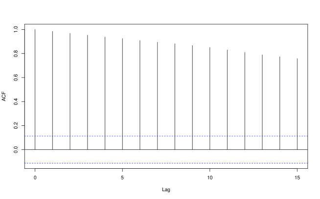
Figure 2: ACF: Bitcoin

It displays local trends, spikes and a long range of serial dependence, displayed in Figure 2, with a linear decay rate resembling a unit root process.

[Insert Figure 2: Bitcoin, ACF]

The data are transformed by substracting its median of 8036.49. Next, the Bitcoin prices are modelled as a noncausal MAR(3,3) process with an unspecified error distribution.

$$(1-\phi_{1}L-\phi_{2}L^{2}-\phi_{3}L^{3})(1-\psi_{1}L^{-1}-\psi_{2}L^{-2}-\psi_{3}L^{-3})y_{t}=\epsilon_{t},$$ (6.3)

where $\epsilon_{t}$ is a strong white noise with a non-Gaussian distribution. The estimation results are reported below:

Table 3. Estimation of MAR(3,3)

parameter	estimate	st.dev
$\psi_{1}$	0.3359	0.0025
$\psi_{2}$	-0.0026	0.0033
$\psi_{3}$	0.0072	0.0021
$\phi_{1}$	0.7029	0.0025
$\phi_{2}$	0.1020	0.0031
$\phi_{3}$	0.1666	0.0020

The parameter estimates are based on the series of errors and their second and third powers. The lag length $H$ is set equal to 3. The standard errors reported in Table 3 are computed from the final Hessian matrix. All estimated parameters (except for $\psi_{2}$) are significant. We observe some causal persistence with the sum of autoregressive coefficients equal to 0.97 and a joint bubble effect with explosive rate of about 3 $\approx\frac{1}{0.3359}$.

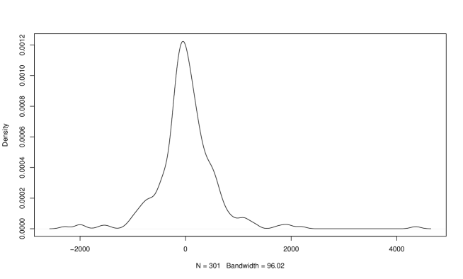
Figure 4: Residuals: Density

The residuals are plotted in Figure 3. We observe that the residuals, unlike the Bitcoin series, do not display a trend. However, they are characterized by two regimes of low and high variance. Figure 4 shows the density of the residuals, where one can observe long tails.

[Insert Figure 3: MAR(3,3) Residuals]

[Insert Figure 4: Residuals, Density]

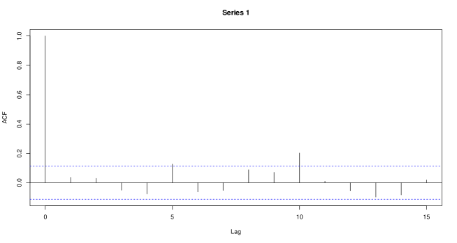
Figure 5: Residuals: ACF

The model MAR(3,3) has almost removed the serial dependence in the data, as shown in the residual ACF showed in Figure 5.

[Insert Figure 4: Residuals, ACF]

The autocorrelation at lag 10 is quite large. However, it is difficult to comment on its significance, given the non-normal and heavy-tailed distribution of the series.

7 Concluding Remarks

In this paper we have introduced a semi-parametric estimation approach for a large class of nonlinear dynamic models with i.i.d. errors. The GCov estimator obtained by minimizing a multivariate portmanteau criterion has semi-parametric efficiency properties for the parameters characterizing the serial dependence. We have also shown that the associated residual-based portmanteau statistic has asymptotically the expected chi-square distribution with an adjusted degree of freedom.

Among further extensions are the following: 1. the approach is based on the knowledge of the asymptotic behavior of the regression coefficient. This behavior is known for errors that do not have finite second order moments [see, Davis, Resnick (1986)]. In such a case the speed of convergence and asymptotic distributions of the GCov estimator are modified. The asymptotic distribution of the (residual-based) portmanteau statistic is modified as well with likely stable limiting distributions [see e.g. Gourieroux, Zakoian (2017)].

2. The set of transformations $a$ could be parametrized. For example, for financial returns we would consider the transformed process $Y_{t}(\lambda)=[sign(y_{t}),|y_{t}|^{\lambda}]$. Then, the GCov estimator can be defined for any $\lambda$ providing a functional estimator $\hat{\theta}(\lambda)$, indexed by $\lambda$. The distribution of this functional estimator can be derived under the null. Then, we could search for the transformation $|y_{t}|^{\lambda^{*}}$ that is the most suitable to represent the dynamic definition of risk.

3. By considering two nested sets of transforms of the series $y_{t}$, and/or different lags, we can build specification tests of the i.i.d. assumption on the errors, i.e. overidentification J-tests [see e.g. Hannan (1967), Hansen (1982), Szroeter (1983), Lanne, Luoto (2021), Section 3.3].

4. The set of transforms can also be used to focus on some features of the error distribution such as the extreme risks [see, Hoga (2021)].

REFERENCES

Ahn, S., and G., Reinsel (1988): ” Nested Reduced Rank Autoregressive Models for Multiple Time Series”, JASA, 89, 849-956.

Anderson, T. (1999): ”Asymptotic Theory for Canonical Correlation Analysis”, Journal of Multivariate Analysis, 70, 1-29.

Anderson, T. (2002): ”Canonical Correlation Analysis and Reduced Rank Regression is Autoregressive Models”, Annals of Statistics, 30, 1134-1154.

Andrews, D. (1987): ”Consistency in Nonlinear Econometric Models: A Generic Uniform Law of Large Numbers”, Econometrica, 55, 1465-1471.

Andrews, B., Breidt, F, and R. Davis (2006): ”Maximum Likelihood Estimation for All Pass Time Series Models”, Journal of Multivariate Analysis, 97, 1638-1659.

Boudjellaba, H., Dufour, J.M. and R. Roy (1994): ”Simplified Conditions for Noncausality Between Vectors in Multivariate ARMA Models”, Journal of Econometrics, 63, 271-287.

Box, G. and D. Pierce (1970): ”Distribution of Residual Autocorrelations in Autoregressive-Integrated Moving Average Time Series Models”, JASA, 65, 1509-1526.

Breidt, J., Davis, R., Lii, K. and M. Rosenblatt (1991): ”Maximum Likelihood Estimation of Noncausal Autoregressive Processes”, Journal of Multivariate Analysis, 36, 175-198.

Chitturi, R. (1974): ”Distribution of Residual Autocorrelations in Multiple Autoregressive Schemes”, JASA, 69, 928-934.

Chitturi, R. (1976): ”Distribution of Multivariate White Noise Autocorrelations”, JASA, 71, 223-226.

Davis, R. and S. Resnick (1986): ”Limit Theory for the Sample Covariance and Correlation Functions of Moving Averages”, Annals of Statistics, 14, 533-558.

Davis, R. and L. Song (2020): ”Noncausal Vector AR Processes with Application to Economic Time Series”, Journal of Econometrics, 216, 246-267.

Duchesne, P. and R. Roy (2003): ”Robust Tests for Independence of Two Time Series”, Statistica Sinica, 13, 827-852.

El Himdi, H. and R. Roy (1997): ”Tests for Noncorrelation of Two Multivariate ARMA Time Series”, Canadian Journal of Statistics, 25, 233-256.

Engle, R. and S. Kozicki (1993): ”Testing for Common Features”, Journal of Business and Economic Statistics”, 11, 369-395.

Engle, R. ,Lilien, D. and R. Robbins (1987): ”Estimating Time Varying Risk Premia in the Term Structure: The ARCH-M Models”, Econometrica, 55, 391-407.

Fisher, T. and C. Gallagher (2012): ”New Weighted Portmanteau Statistic for Time Series Goodness of Fit Testing”, JASA, 107, 777-787.

Forrester, P. and J. Zhang (2020): ”Parametrizing Correlation Matrices”, Journal of Multivariate Analysis, 178, 104619.

Francq, C., Roy, R. and J.M. Zakoian (2005): ”Diagnostic Checking in ARMA Models with Uncorrelated Errors”, JASA, 100, 532-544.

Gourieroux, C. and J. Jasiak (2016): ”Filtering, Prediction and Simulation Methods for Noncausal Processes”, Journal of Time Series Analysis, 37, 405-430.

Gourieroux, C. and J. Jasiak (2017): ”Noncausal Vector Autoregressive Process: Representation, Identification and Semi-Parametric Estimation”, Journal of Econometrics, 200, 118-134.

Gourieroux, C. and A. Monfort (1995): ” Statistics and Econometric Models”, Vol 2, Cambridge Univ. Press.

Gourieroux, C., Monfort, A. and J.P. Renne (2020): ”Identification and Estimation in NonFundamental Structural VARMA Models”, Review of Economic Studies, 87, 1915-1953.

Gourieroux, C. and J.M. Zakoian (2017): ”Local Explosion Modelling by Non-Causal Process”, JRSS B, 79, 737-756.

Hannan, J. (1967): ”Canonical Correlation and Multiple Equation Systems in Economics”, Econometrica, 35, 123-138.

Hannan, J. (1976): ”The Asymptotic Distribution of Serial Covariances”, Annals of Statistics, 4, 396-399.

Hansen, L. (1982): ”Large Sample Properties of Generalized Method of Moment Estimators”, Econometrica, 50, 1029-1054.

Haugh, L. (1976): ”Checking the Independence of Two Covariance-Stationary Time Series: A Univariate Residual Cross-Correlation Approach”, JASA, 71, 378-385.

Hecq, A., Lieb, L. and S. Telg (2016): ”Identification of Mixed Causal-Noncausal Models in Finite Samples”, Annals of Economics and Statistics, 123/124, 307-331.

Hoga, Y. (2021): ”Testing for Serial Extreme Dependence in Time Series Residuals”, D.P. University of Duisburg-Essen.

Horn, R. and C. Johnson (1999): ”Topics in Matrix Analysis”, Cambridge University Press.

Hosking, J. (1980): ”The Multivariate Portmanteau Statistic”, JASA, 75, 602-608.

Hosking, J. (1981)a: ”Equivalent Forms of the Multivariate Portmanteau Statistic”, JRSS B, 43, 261-262.

Hosking, J. (1981)b: ”Lagrange Multiplier Tests of Multivariate Time Series Models”, JRSS B, 43, 219-230.

Hotelling, H. (1936) : ”Relation Between Two Sets of Variants”, Biometrika, 28, 321-377.

Huber, P. (1967): ” The Behaviors of Maximum Likelihood Estimators Under Nonstandard Conditions”, Proceeding of the Fifth Berkeley Symposium on Mathematical Statistics and Probability, Vol 1, 221-253.

Jennrich, R. (1969): ”Asymptotic Properties of Nonlinear Least Squares”, Annals of Mathematical Statistics, 40, 633-643.

Jin, Z. and D. Matteson (2018): ”Generalizing Distance Covariance to Measure and Test Multivariate Mutual Dependence via Complete and Incomplete V-Statistics”, Journal of Multivariate Analysis, 168, 304-322.

Kettenring, J. (1971): ”Canonical Analysis of Several Sets of Variables”, Biometrika, 58, 433-451.

Lam, C. and Q. Yao (2012): ”Factor Modelling for High Dimensional Time Series”, Biometrika, 98, 901-918.

Lanne, M., and J. Luoto (2021): ”GMM Estimation of Non-Gaussian Structural Vector Autoregression”, Journal of Business and Economic Statistics, 39, 69-81.

Lanne, M., and P. Saikkonen (2010): ”Noncausal Autoregressions for Economic Time Series”, Journal of Time Series Econometrics, 3, 1-39.

Lanne, M., and P. Saikkonen (2011): ”GMM Estimators with Non-Causal Instruments”, Oxford Bulletin of Economics and Statistics, 71, 581-591.

Lanne, M., and P. Saikkonen (2013): ” Noncausal Vector Autoregression”, Econometric Theory, 29, 447-481.

Li, W. and A. McLeod (1981): ”Distribution of the Residual Autocorrelations in Multivariate ARMA Time Series Models”, JRSS B, 43, 231-233.

Li, W. and T. Mak (1994): ”On the Squared Residual Autocorrelations in Nonlinear Time Series with Conditional Heteroscedasticity”, JTSA, 15, 627-639.

Lin, J. and A. McLeod (2006): ”Improved Pena-Rodriguez Portmanteau Test”, Computational Statistics and Data Analysis, 51, 1731-1738.

Ling, S and W. Li (1997): ”On Fractionally Integrated Autoregressive Moving Average Time Series Models with Conditional Heteroscedasticity”, JASA, 92, 1184-1194.

Ljung, G. and G. Box (1978): ”On the Measure of Lack of Fit in Time Series Models”, Biometrika, 65, 297-303.

Magnus, J. and H. Neudecker (2019): ” Matrix Differential Calculus with Applications in Statistics and Econometrics”, Wiley.

Mahdi, E. and I. McLeod (2012): ”Improved Multivariate Portmanteau Test”, Journal of Time Series Analysis”, 23, 211-222.

Mann, H. and A. Wald (1943): ”On the Statistical Treatment of Linear Stochastic Difference Equations”, Econometrica, 11, 173-220.

Neuenschwander, B. and B. Flury (1995): ”Common Canonical Variates”, Biometrika, 82, 553-560.

Niu, L., Liu, X. and J. Zhao (2020): ”Robust Estimators of the Correlation Matrix with Sparse Kronecker Structure for a High Dimensional Matrix Variate”, Journal of Multivariate Analysis, 177, 104598.

Pena, D. and J. Rodriguez (2002): ”A Powerful Portmanteau Test of Lack of Fit for Time Series”, JASA, 97, 601-610.

Pena, D. and J. Rodriguez (2006): ”The Log of the Determinant of the Autocorrelation Matrix for Testing Goodness of Fit in Time Series”, Journal of Statistical Planning and Inference, 136, 2706-2718.

Reinsel, G. and R. Velu (1998): ”Multivariate Reduced Rank Regressions”, Springer, New York.

Robinson, P. (1973): ” Generalized Canonical Analysis for Time Series”, Journal of Multivariate Analysis, 3, 141-160.

Sims, C. (2021): ”SVAR Identification through Heteroscedasticity with Misspecified Regimes”, Princeton, DP.

Szroeter, J. (1983): ”Generalized Wald Methods for Testing Nonlinear Implicit and Overidentifying Restrictions”, Econometrica, 51, 335-353,

Velu, R., Reinsel, G. and D. Wichern (1986): ”Reduced Rank Models for Multiple Time Series”, Biometrika, 73, 109-118.

White, H. (1982): ”Maximum Likelihood Estimation of Misspecified Models”, Econometrica, 50, 1-25.

Wooldridge, J. (1991): ”On the Application of Robust Regression-Based Diagnostics to Models of Conditional Means and Conditional Variances”, Journal of Econometrics, 47, 5-46.

Yata, K., and M. Aoshima (2016): ”High Dimensional Inference on Covariance Structures via the Extended Cross-Data Matrix Methodology”, Journal of Multivariate Analysis, 151, 151-166.

Figure 1: Bitcoin, Daily Closing Prices

Figure 3: MAR(3,3) Residuals

APPENDIX 1

The SUR Interpretation

Let us consider the VAR(1) representation:

$$Y_{t}=\alpha+BY_{t-1}+u_{t},$$

where $E(u_{t})=0$, $V(u_{t})=\Sigma$, and $\Sigma$ is invertible.

This is a SUR model with identical regressors $X_{t}=Y_{t-1}$ in all equations. It is well-known that the GLS estimator of $B$ is obtained by applying the OLS equation by equation. Then, we have:

$$\hat{B}=\hat{\Gamma}(1)\hat{\Gamma}(0)^{-1}\iff\hat{B}^{\prime}=\hat{\Gamma}(0)^{-1}\hat{\Gamma}(1)^{\prime}.$$

Moreover, we have asymptotically

$$\sqrt{T}[vec(\hat{B}^{\prime})-vecB^{\prime}]\approx N[0,\Sigma\otimes\Gamma(0)^{-1}],$$ (a.1)

where the $\otimes$ denotes the Kronecker product [see e.g. Chitturi (1974), eq. (1.13)]. In particular, under the null hypothesis $H_{0}=(\Gamma(1)=0)=(B=0)$, we have $\Sigma=\Gamma(0)$ and

$$\sqrt{T}vec(B^{\prime})\sim N(0,\Gamma(0)\otimes[\Gamma(0)^{-1}]).$$ (a.2)

Therefore, the Lagrange Multiplier test statistic for testing $H_{0}$ is:

$$\xi(1) = Tvec[\hat{\Gamma}(0)^{-1}\hat{\Gamma}(1)^{\prime}]^{\prime}[\hat{\Gamma}(0)^{-1}\otimes\hat{\Gamma}(0)]vec[\hat{\Gamma}(0)^{-1}\hat{\Gamma}(1)^{\prime}]$$

$$= Tvec[\hat{\Gamma}(0)^{-1}\hat{\Gamma}(1)^{\prime}]^{\prime}[\hat{\Gamma}(0)^{-1/2}\otimes\hat{\Gamma}(0)^{1/2}][\hat{\Gamma}(0)^{-1/2}\otimes\hat{\Gamma}(0)^{1/2}]vec[\hat{\Gamma}(0)^{-1}\hat{\Gamma}(1)^{\prime}]$$

$$= Tvec[\hat{\Gamma}(0)^{-1/2}\hat{\Gamma}(1)^{\prime}\hat{\Gamma}(0)^{-1/2}]^{\prime}vec[\hat{\Gamma}(0)^{-1/2}\hat{\Gamma}(1)^{\prime}\hat{\Gamma}(0)^{-1/2}],$$

by using the equality: $vec(ABC)=(C^{\prime}\otimes A)vecB$ [see e.g. Lemma 4.3.1 in Horn, Johnson (1999), or Magnus, Neudecker (2019), ch. 18, p. 440-441]. Moreover, we have $[vecC]^{\prime}[vecC]=Tr\;CC^{\prime}$. Therefore,

$$\xi(1) = T\;Tr[\hat{\Gamma}(0)^{-1/2}\hat{\Gamma}(1)^{\prime}\hat{\Gamma}(0)^{-1}\hat{\Gamma}(1)\hat{\Gamma}(0)^{-1/2}]$$ (a.3)

$$= T\;Tr[\hat{\Gamma}(1)^{\prime}\hat{\Gamma}(0)^{-1}\hat{\Gamma}(1)\hat{\Gamma}(0)^{-1}]$$

$$= T\;Tr\hat{R}^{2}(1).$$

Remark: We easily deduce from (a.2) the asymptotic distribution of $\sqrt{T}vec[\hat{\Gamma}(1)^{\prime}]$ [see also Chitturi (1976), Hannan(1976)]. Indeed, we have:

$$\sqrt{T}\hat{\Gamma}(1)^{\prime}=\hat{\Gamma}(0)\sqrt{T}\hat{B}^{\prime}\approx\Gamma(0)\sqrt{T}\hat{B}^{\prime},$$

and then

$$vec[\sqrt{T}\hat{\Gamma}(1)^{\prime}]=vec[\Gamma(0)\sqrt{T}\hat{B}^{\prime}]=[Id\otimes\Gamma(0)]vec(\sqrt{T}\hat{B}^{\prime}).$$

It follows that:

$$vec[\sqrt{T}\hat{\Gamma}(1)^{\prime}] \approx N[0,[Id\otimes\Gamma(0)][\Gamma(0)\otimes\Gamma(0)^{-1}][Id\otimes\Gamma(0)]]$$

$$= N[0,\Gamma(0)\otimes\Gamma(0)].$$

APPENDIX 2

Asymptotic Expansions

A.2.1 First-Order Derivative of $Tr\,R^{2}(1;\theta)$

At lag $h=1$, we have

$$Tr\,R^{2}(1;\theta)=Tr[\Gamma(1;\theta)\Gamma(0;\theta)^{-1}\Gamma(1;\theta)^{\prime}\Gamma(0,\theta)^{-1}].$$

The first-order partial derivatives are computed by considering the differential:

$$d\,Tr\,R^{2}(1;\theta)=\sum_{j=1}^{J}\frac{\partial Tr\,R^{2}(1;\theta)}{\partial\theta_{j}}d\theta_{j}.$$

We have:

$$d\,Tr\,R^{2}(1;\theta) = Tr[d\Gamma(1;\theta)\Gamma(0;\theta)^{-1}\Gamma(1;\theta)^{\prime}\Gamma(0,\theta)^{-1}]$$

$$+ Tr[\Gamma(1;\theta)d[\Gamma(0;\theta)^{-1}]\Gamma(1;\theta)^{\prime}\Gamma(0,\theta)^{-1}]$$

$$+ Tr[\Gamma(1;\theta)\Gamma(0;\theta)^{-1}d\Gamma(1;\theta)^{\prime}\Gamma(0,\theta)^{-1}]$$

$$+ Tr[\Gamma(1;\theta)\Gamma(0;\theta)^{-1}\Gamma(1;\theta)^{\prime}d[\Gamma(0,\theta)^{-1}]],$$

because

$d[A(\theta)B(\theta)]=dA(\theta)B(\theta)+A(\theta)dB(\theta)$ and $d\,Tr[A(\theta)+B(\theta)]=Tr\,[dA(\theta)+dB(\theta)]$. In addition, we know that $Tr\,(AB)=Tr\,(BA),Tr\,A^{\prime}=Tr\,A$. Hence,

$$d\,Tr\,[R^{2}(1;\theta)] = Tr\,[\Gamma(0;\theta)^{-1}\Gamma(1;\theta)^{\prime}\Gamma(0;\theta)^{-1}d\Gamma(1;\theta)]$$

$$+ Tr\,[\Gamma(1;\theta)^{\prime}\Gamma(0;\theta)^{-1}\Gamma(1;\theta)d[\Gamma(0;\theta)^{-1}]]$$

$$+ Tr\,[d\Gamma(1;\theta)^{\prime}\Gamma(0;\theta)^{-1}\Gamma(1;\theta)\Gamma(0;\theta)^{-1}]$$

$$+ Tr\,[\Gamma(1;\theta)\Gamma(0;\theta)^{-1}\Gamma(1;\theta)^{\prime}d[\Gamma(0;\theta)^{-1}]$$

$$= 2Tr\,[\Gamma(0;\theta)^{-1}\Gamma(1;\theta)^{\prime}\Gamma(0;\theta)^{-1}d\Gamma(1;\theta)]$$

$$+ Tr\,\left[[\Gamma(1;\theta)^{\prime}\Gamma(0;\theta)^{-1}\Gamma(1;\theta)+\Gamma(1;\theta)\Gamma(0;\theta)^{-1}\Gamma(1;\theta)^{\prime}]d[\Gamma(0;\theta)^{-1}]\right].$$

We have:

$$d[A(\theta)^{-1}]=-A(\theta)^{-1}dA(\theta)A(\theta)^{-1}.$$

Next, let us substitute this expression into the formula of $d\,Tr\,[R^{2}(1;\theta)]$:

$$d\,Tr\,R^{2}(1;\theta) = 2\,Tr\,[\Gamma(0;\theta)^{-1}\Gamma(1;\theta)^{\prime}\Gamma(0;\theta)^{-1}d\Gamma(1;\theta)]$$ (a.4)

$$- Tr\,\left[\Gamma(0;\theta)^{-1}[\Gamma(1;\theta)^{\prime}\Gamma(0;\theta)^{-1}\Gamma(1;\theta)+\Gamma(1;\theta)\Gamma(0;\theta)^{-1}\Gamma(1;\theta)^{\prime}]\Gamma(0;\theta)^{-1}d\Gamma(0;\theta)\right]$$

$$= 2Tr\,[\Gamma(0;\theta)^{-1}\Gamma(1;\theta)^{\prime}\Gamma(0;\theta)^{-1}d\Gamma(1;\theta)]$$

$$- Tr\,\left[[\tilde{R}^{2}(1;\theta)\Gamma(0;\theta)^{-1}+\Gamma(0;\theta)^{-1}R^{2}(1;\theta)]d\Gamma(0;\theta)\right],$$

with

$$\tilde{R}^{2}(1;\theta)=\Gamma(0;\theta)^{-1}\Gamma(1;\theta)^{\prime}\Gamma(0;\theta)^{-1}\Gamma(1;\theta).$$ (a.5)

A.2.2. First-Order Conditions (FOC)

The First-Order Conditions are:

$$\frac{\partial Tr\,\hat{R}^{2}(1;\theta_{j})}{\partial\theta_{j}}=0,\;j=1,...,J=dim\theta$$ (a.6)

$$\iff 2\,Tr[\hat{\Gamma}(0;\theta)^{-1}\hat{\Gamma}(1;\theta)^{\prime}\hat{\Gamma}(0;\theta)^{-1}\frac{\partial\hat{\Gamma}(1;\theta)}{\partial\theta_{j}}]$$

$$-Tr\{\,[\hat{\tilde{R}}^{2}(1;\theta)\hat{\Gamma}(0;\theta)^{-1}+\hat{\Gamma}(0;\theta)^{-1}\hat{R}^{2}(1,\theta)]\frac{\partial\hat{\Gamma}(0;\theta)}{\partial\theta_{j}}\}=0,$$

$$\;j=1,...,J=dim\theta.$$

A.2.3. Second–Order Expansion

We can derive the first-order conditions (FOC) in the neighborhood of $\hat{\theta}\approx\theta_{0}$. For some matrix function $A(\theta)$ of $\theta$, we consider the differential defined by:

$$dA(\theta)=\sum_{j=1}^{J}\frac{\partial A(\theta)}{\partial\theta_{j}}d\theta_{j},$$

with $d\theta_{j}=\hat{\theta}_{j}-\theta_{j0}$. From (a,6), we get:

$$dFOC_{j}(\theta) = 2Tr\,\left[\frac{\partial\hat{\Gamma}(1,\theta)}{\partial\theta_{j}}\,d[\hat{\Gamma}(0;\theta)^{-1}\hat{\Gamma}(1;\theta)^{\prime}\hat{\Gamma}(0;\theta)^{-1}]\right]$$ (a.7)

$$+ 2\left[\hat{\Gamma}(0;\theta)^{-1}\hat{\Gamma}(1;\theta)^{\prime}\hat{\Gamma}(0;\theta)^{-1}d[\frac{\partial\hat{\Gamma}(1;\theta)}{\partial\theta_{j}}]\right]$$

$$- Tr\,\left[\hat{\tilde{R}}^{2}(1;\theta)\hat{\Gamma}(0;\theta)^{-1}+\hat{\Gamma}(0;\theta)^{-1}\hat{R}^{2}(1;\theta)\right]\,d[\frac{\partial\hat{\Gamma}(0;\theta)}{\partial\theta_{j}}]$$

$$- Tr\,\{[\frac{\partial\hat{\Gamma}(0,\theta)}{\partial\theta_{j}}]\,d[\hat{\tilde{R}}^{2}(1;\theta)\hat{\Gamma}(0;\theta)^{-1}+\hat{\Gamma}(0;\theta)^{-1}\hat{R}^{2}(1;\theta)]\}.$$

In the above expression the terms without differential have to be evaluated at $\theta=\theta_{0}$.

The expressions involving differential term $d[.]$ are linear with respect to $\hat{\theta}-\theta_{0}$ and then of order $1/\sqrt{T}$. Moreover, for $\theta=\theta_{0}$, we have $\Gamma(0;\theta_{0})$ invertible, $\Gamma(1;\theta_{0})=0$. Therefore $\hat{\Gamma}(0;\theta_{0})$ is of order 1 and $\hat{\Gamma}(1;\theta_{0})$ of order $1/\sqrt{T}$. We deduce that the second and third components of the right hand side of the above equation (a.7) evaluated at $\theta=\theta_{0}$ are negligible with respect to the other components. Then, the right hand side of equation (a.7) can be replaced by:

$$2Tr\,\left[\frac{\partial\hat{\Gamma}(1,\theta_{0})}{\partial\theta_{j}}\,d[\hat{\Gamma}(0;\theta)^{-1}\hat{\Gamma}(1;\theta)^{\prime}\hat{\Gamma}(0;\theta)^{-1}]\right]$$

$$- Tr\left[\frac{\partial\Gamma(0,\theta_{0})}{\partial\theta_{j}}d[\hat{\Gamma}(0;\theta)^{-1}\hat{\Gamma}(1,\theta)^{\prime}\hat{\Gamma}(0;\theta)^{-1}\hat{\Gamma}(1,\theta)+\hat{\Gamma}(1,\theta)\hat{\Gamma}(0,\theta)^{-1}\hat{\Gamma}(1,\theta)^{\prime}\hat{\Gamma}(0;\theta)^{-1}]\right].$$

i) The matrix $J(\theta)$

Next, we use $d[A(\theta)B(\theta)]=[dA(\theta)]B(\theta)+A(\theta)[dB(\theta)]$. Let us consider the limiting FOC, when the sample autocovariances are replaced by their theoretical counterparts and use $\Gamma(1;\theta_{0})=0$. We get:

$$dFOC_{j}(\theta)=2Tr\,[\frac{\partial\Gamma(1;\theta_{0})}{\partial\theta_{j}}\,\Gamma(0;\theta_{0})^{-1}d\Gamma(1;\theta)^{\prime}\Gamma(0;\theta_{0})^{-1}]$$

$$- Tr[\frac{\partial\Gamma(0,\theta_{0})}{\partial\theta_{j}}[\Gamma(0;\theta_{0})^{-1}d\Gamma(1,\theta)^{\prime}\Gamma(0;\theta_{0})^{-1}\Gamma(1,\theta_{0})$$

$$+ \Gamma(0,\theta_{0})^{-1}\Gamma(1,\theta_{0})^{\prime}\Gamma(0,\theta_{0})^{-1}d\Gamma(1,\theta)+d\Gamma(1,\theta)^{\prime}\Gamma(0;\theta_{0})^{-1}\Gamma(1,\theta_{0})^{\prime}\Gamma(0,\theta_{0})^{-1}$$

$$+ \Gamma(1,\theta_{0})\Gamma(0;\theta_{0})^{-1}d\Gamma(1,\theta)^{\prime}\Gamma(0;\theta_{0})^{-1}]]$$

$$= 2\,Tr\,[\frac{\partial\Gamma(1;\theta_{0})}{\partial\theta_{j}}\Gamma(0;\theta_{0})^{-1}d\Gamma(1;\theta)^{\prime}\Gamma(0;\theta_{0})^{-1}].$$

The matrix $J(\theta_{0})$ of second-order derivatives has elements $(j,k)$ such that:

$$-J_{jk}(\theta_{0})=2Tr\,\left[\frac{\partial\Gamma(1;\theta_{0})}{\partial\theta_{j}}\Gamma(0;\theta_{0})^{-1}\frac{\partial\Gamma(1;\theta_{0})^{\prime}}{\partial\theta_{k}}\Gamma(0;\theta_{0})^{-1}\right],\;\forall j,k,$$

or, equivalently:

$$J(\theta_{0})=-2\frac{\partial vec\Gamma(1;\theta_{0})^{\prime}}{\partial\theta}[\Gamma(0;\theta_{0})^{-1}\otimes\Gamma(0;\theta_{0})^{-1}]\frac{\partial vec\Gamma(1;\theta_{0})}{\partial\theta^{\prime}}.$$ (a.8)

ii) Asymptotic equivalence for $\sqrt{T}(\hat{\theta}_{T}-\theta_{0})$ (written for $H=1$)

Hence we have:

$\sqrt{T}[\hat{\theta}_{T}-\theta_{0}]=J(\theta_{0})^{-1}\sqrt{T}\frac{dL_{T}(\theta)}{d\theta}=$ $J(\theta_{0})^{-1}\sqrt{T}X(\hat{\Gamma})+o_{p}(1)$, where by (a.6):

$$X_{j}(\hat{\Gamma})=2Tr[\hat{\Gamma}(0;\theta_{0})^{-1}\hat{\Gamma}(1,\theta_{0})^{\prime}\hat{\Gamma}(0;\theta_{0})^{-1}\frac{\partial\hat{\Gamma}(1,\theta_{0})}{\partial\theta_{j}}]$$

$$- Tr\,\{[\hat{\tilde{R}}^{2}(1;\theta_{0})\hat{\Gamma}(0;\theta_{0})^{-1}+\hat{\Gamma}(0;\theta_{0})^{-1}\hat{R}^{2}(1;\theta_{0})]\frac{\partial\hat{\Gamma}(1,\theta_{0})}{\partial\theta_{j}}\},$$

by (a.6). It is Normally distributed as $\hat{\Gamma}\approx\Gamma$ with the Central Limit Theorem that holds for the sample autocovariances.

We have $X_{j}(\hat{\Gamma})-X_{j}(\Gamma)=dX_{j}(\Gamma)$. We can disregard all terms including $\Gamma(1,\theta_{0})$ as $\Gamma(1;\theta_{0})=0$. Hence,

$$\sqrt{T}X_{j}(\hat{\Gamma}) \approx 2Tr\,[\Gamma(0;\theta_{0})^{-1}\sqrt{T}\hat{\Gamma}(1;\theta_{0})\Gamma(0;\theta_{0})^{-1}\frac{\partial\Gamma^{\prime}(1;\theta_{0})}{\partial\theta_{j}}]$$

$$\approx 2Tr\,[\Gamma(0;\theta_{0})^{-1}\frac{\partial\Gamma^{\prime}(1;\theta_{0})}{\partial\theta_{j}}\Gamma(0;\theta_{0})^{-1}\sqrt{T}\hat{\Gamma}(1;\theta_{0})],$$

by applying $Tr\,A^{\prime}=Tr\,A$ and $Tr(AB)=Tr(BA)$.

Since $Tr\,(A^{\prime}B)=(vecA)^{\prime}(vecB)$ and $vec(A\otimes C)=(C^{\prime}\otimes A)$, we deduce:

$$\sqrt{T}X_{j}(\hat{\Gamma}) \approx 2vec[\Gamma(0;\theta_{0})^{-1}\frac{\partial\Gamma(1;\theta_{0})}{\partial\theta_{j}}\Gamma(0;\theta_{0})^{-1}]^{\prime}vec[\sqrt{T}\hat{\Gamma}^{\prime}(1;\theta_{0})]$$

$$= A_{j}(\theta)vec[\sqrt{T}\hat{\Gamma}^{\prime}(1;\theta_{0})],\;j=1,...,J=dim\theta.$$

or,

$$\sqrt{T}X(\hat{\Gamma})=A(\theta)vec[\sqrt{T}\hat{\Gamma}^{\prime}(1;\theta_{0})],$$

where

$$A(\theta)=2\frac{\partial vec\Gamma(1;\theta)^{\prime}}{\partial\theta}\left[\Gamma(0;\theta_{0})^{-1}\otimes\Gamma(0;\theta_{0})^{-1}\right].$$ (a.9)

From the remark in Appendix 1, it follows that:

$$vec[\sqrt{T}\hat{\Gamma}^{\prime}(1;\theta_{0})]\approx N[0,\Gamma(0;\theta_{0})\otimes\Gamma(0;\theta_{0})].$$

Therefore $\sqrt{T}X(\hat{\Gamma})$ is asymptotically normally distributed, with mean zero and asymptotic variance:

$$V_{asy}[\sqrt{T}X(\hat{\Gamma})]=-2J(\theta_{0}).$$ (a.10)

From (a.10), and the absence of correlation between the matrices $\hat{\Gamma}(h)$ at different lags, we deduce the simplification in deriving the asymptotic variance-covariance matrix of $\sqrt{T}(\hat{\theta}_{T}-\theta_{0})$ in Corollary 1.

APPENDIX 3

Expansion of the Multivariate Portmanteau Statistic

(i) Let us consider the asymptotic expansion of:

$$TL_{T}(\theta_{0})=T\,Tr\,[\hat{\Gamma}(1;\theta_{0})\hat{\Gamma}(0;\theta_{0})^{-1}\hat{\Gamma}(1;\theta_{0})^{\prime}\hat{\Gamma}(0;\theta_{0})^{-1}],$$

written for $H=1$. Since $Tr(C^{\prime}C)=[vec\,C]^{\prime}[vec\,C]$, we have:

$$TL_{T}(\theta_{0})=Tvec[\hat{\Gamma}(1;\theta_{0})^{\prime}\hat{\Gamma}(0;\theta_{0})^{-1}]^{\prime}vec[\hat{\Gamma}(1;\theta_{0})^{\prime}\hat{\Gamma}(0;\theta_{0})^{-1}].$$

Moreover, since $vec(ABC)=(C^{\prime}\otimes A)vecB$, we get:

$$TL_{T}(\theta_{0}) \approx [\sqrt{T}vec\hat{\Gamma}^{\prime}(1;\theta_{0})]^{\prime}[\Gamma(0;\theta_{0})^{-1}\otimes\Gamma(0;\theta_{0})^{-1}][\sqrt{T}vec\hat{\Gamma}^{\prime}(1;\theta_{0})].$$

(ii) Then, let us consider the asymptotic expansion (5.2) of the standardized residual-based portmanteau statistic. By using (a.8), (a.9) and the above result, we get:

$$TL_{T}(\hat{\theta}_{T})\approx vec[\sqrt{T}\hat{\Gamma}^{\prime}(1;\theta_{0})^{\prime}]^{\prime}\,\Pi\,vec[\sqrt{T}\hat{\Gamma}^{\prime}(1;\theta_{0})^{\prime}],$$ (a.11)

with

$$\Pi = \Gamma(0;\theta_{0})^{-1}\otimes\Gamma(0;\theta_{0})^{-1}$$ (a.12)

$$- [\Gamma(0;\theta_{0})^{-1}\otimes\Gamma(0;\theta_{0})^{-1}]\frac{\partial vec\Gamma(1;\theta_{0})}{\partial\theta^{\prime}}$$

$$\left\{\frac{\partial vec\Gamma(1;\theta_{0})^{\prime}}{\partial\theta}[\Gamma(0;\theta_{0})^{-1}\otimes\Gamma(0;\theta_{0})^{-1}]\frac{\partial vec\Gamma(1;\theta_{0})}{\partial\theta}\right\}^{-1}$$

$$\frac{\partial vec\Gamma(1;\theta_{0})^{\prime}}{\partial\theta}[\Gamma(0;\theta_{0})^{-1}\otimes\Gamma(0;\theta_{0})^{-1}].$$

(iii) The condition

$$\Pi\,V_{asy}[\sqrt{T}\,vec\hat{\Gamma}(1;\theta_{0})^{\prime}]\,\Pi=\Pi,$$

with $V_{asy}\sqrt{T}\,vec[\hat{\Gamma}(1;\theta_{0})^{\prime}]=\Gamma(0;\theta_{0})\otimes\Gamma(0;\theta_{0})$ is verified. It is due to an interpretation in terms of orthogonal projection of $vec[\sqrt{T}\hat{\Gamma}^{\prime}(1;\theta_{0})^{\prime}]$ on the $\partial vec\Gamma(1;\theta_{0})^{\prime}/\partial\theta$ for the scalar product associated with $\Gamma(0;\theta_{0})\otimes\Gamma(0;\theta_{0})$.