Gluing Karcher–Scherk saddle towers II:
Singly periodic minimal surfaces

Abstract.

This is the second in a series of papers that construct minimal surfaces by gluing singly periodic Karcher–Scherk saddle towers along their wings. This paper aims to construct singly periodic minimal surfaces with Scherk ends. As in the first paper, we prescribe phase differences between saddle towers, and obtain many new examples without any horizontal reflection plane. This construction is not very different from previous ones, hence we will only provide sketched proofs.

We will however study the embeddedness with great care. Previously, embeddedness can not be determined in the presence of “parallel” Scherk ends, as it was not clear if they bend towards or away from each other. In a recent study, the bending was completely ignored and embeddedness was falsely claimed. We correct this mistake by carefully analysing slight bendings, thus identify scenarios where the constructed surfaces are indeed embedded.

1. Introduction

In [Tra01], Traizet desingularized arrangements of vertical planes into singly periodic minimal surfaces (SPMSs) using the node-opening technique: Scherk towers are placed at the intersection lines and are glued along their wings. However, the construction relied on many assumptions: (1) The arrangement was assumed to be simple in the sense that no three planes intersect in a line; (2) The minimal surface was assumed to be symmetric in a horizontal plane; (3) For the surfaces to be embedded, it was assumed that no two planes are parallel. The purpose of this paper is to get rid of these assumptions as far as we can.

On the one hand, we will consider a larger family of configurations. More specifically, let $\Gamma$ be a “graph” which, informally speaking, consists of straight segments and rays (edges) that intersect only at their endpoints (vertices). We will desingularize $\Gamma\times\mathbb{R}$ into a minimal surface by placing Karcher–Scherk saddle towers over the vertices and glue them along their wings following the pattern of the graph. In particular, the minimal surface has Scherk ends corresponding to the rays of the graph.

On the other hand, we will remove the horizontal reflection plane. This is done, as in the first paper, by prescribing phase differences between saddle towers. Our main result (Theorem 2 below) is then analogous to that of the first paper [CT21]: The gluing construction sketched above produces a continuous family of immersed SPMSs only when the graph satisfies a horizontal balancing condition, and the phases of the saddle towers satisfy a subtle vertical balancing condition. Consequently, we obtain many examples without any reflectional symmetry; see Section 3.3. They provide a negative answer to a question in [Tra96] that asks whether every SPMS with Scherk ends has a horizontal reflection plane.

Remark 1.

The first SPMSs with Scherk ends but no horizontal reflection plane were explicitly constructed in [MRB06] with a very different technique. Our construction demonstrates that Traizet’s node-opening technique [Tra01] is flexible and powerful in producing implicit non-symmetric examples.

In this paper, we will only sketch the gluing construction, as all technical details can be found in the first paper [CT21] or even earlier works, and we do not want to repeat ourselves. The readers are therefore expected to have a reasonable familiarity with the first paper.

Our main concern is the embeddedness, especially when the graph $\Gamma$ has parallel rays. In [Tra01], the embeddedness was only guaranteed in the absence of parallel vertical planes because, otherwise, the corresponding Scherk ends risk to bend towards each other after desingularization, therefore create self-intersection.

In some recent work [Mor20], the bendings of Scherk ends were completely ignored and embedded SPMSs with “parallel” Scherk ends were falsely claimed. We are therefore compelled to provide a proper technical treatment on the bendings. Indeed, our construction allows quantitative detections of very slight bendings, thus helps to resolve very delicate embeddedness.

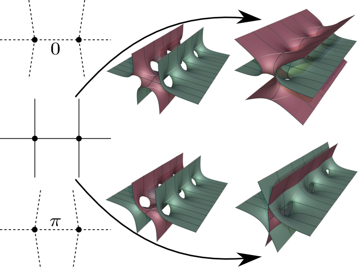
Figure 1. The simple graph on the left gives rise to SPMSs with two saddle towers that are glued either in phase or in opposite phases. If they are in phase, the surfaces are embedded after desingularization, as shown in the figures on the top. If they are in opposite phases, the surfaces are not embedded, as shown in the figures in the bottom.

We identify two types of bending. The first arise from the horizontal deformations, as the saddle towers expand and the glued wings shrink. We will explicitly describe this deformation to the lowest order; see Theorem 4. However, in the case of simple vertical plane arrangment [Tra01], for example, this deformation does not help determine embeddedness.

We are then obliged to consider a very subtle type of bending, arising from the need to balance slight variations of the horizontal forces. This bending is very delicate. We will see that, while the expansion of saddle towers and shrinking of the glued wings are of the order $\varepsilon^{2}$, the variations of the horizontal forces, as well as the deformations they cause, are of the order $\exp(-\ell/\varepsilon^{2})$, where $\ell$ is the shortest edge length in the graph. It is therefore understandable that these bendings could be easily ignored. Again we will explicitly describe this deformation to the lowest order; see Theorem 6.

Example 1.

Figure 1 shows the simplest example that demonstrates the subtle bending. The graph appears as an arrangement of three lines, one horizontal and two vertical. So we will glue two Scherk saddle towers along a single pair of wings. We will see in Lemma 3 that the two saddle towers are either in phase or in opposite phases. Contrary to what was claimed in [Mor20], the Scherk ends will not remain parallel after desingularization. If the saddle towers are in phase, the force along the glued wings will increase, and the Scherk ends must bend away from each other to preserve balance, so the resulting surfaces are embedded. If they are in opposite phases, the force will decrease, and the Scherk ends must bend towards each other, so the resulting surfaces are not embedded. We will revisit this example in Section 3.1. ∎

The paper is organized as follows. In Section 2, we set up the graph theoretical language before using it to state our main results. Examples are given in Section 3. Section 4 is dedicated to the constructions and proofs.

The construction of the immersed families will only be sketched, as the technical details can be found in the first paper of this series [CT21]. Only the proof of embeddedness (Section 4.4), especially in the case of simple vertical plane arrangement (Section 4.4.4), will be given in detail, because the involved technique can not be found in previous works.

Acknowledgement

I appreciate the quick and friendly response from Fillippo Morabito upon learning Example 1. He has acknowledged the existence of mistake in [Mor20].

All 3D pictures in this paper are from http://minimalsurfaces.blog, an online repository maintained by Matthias Weber, to whom I express my gratitude. I also thank Peter Connor who pointed me to some known examples that arise from our construction.

2. Main result

2.1. Graph theory

We define a pseudo rotation system as a triplet $(\mathsf{H},\iota,\varsigma)$ where $\mathsf{H}$ is a finite set of half-edges, $\iota$ and $\varsigma$ are two permutations acting on $\mathsf{H}$, $\iota$ is an involution, and the group generated by $\iota$ and $\varsigma$ acts transitively on $\mathsf{H}$. Note that $(\mathsf{H},\iota,\varsigma)$ is not a rotation system (hence “pseudo”) because we allow the involution $\iota$ to have fixed points. We use $\mathsf{R}$ to denote the set of fixed points of $\iota$.

In analogy to the rotation systems that define multigraphs, a pseudo rotation system defines a graph-like structure $(\mathsf{H},\mathsf{V},\mathsf{E})$, where the vertex set $\mathsf{V}$ consists of the orbits of $\varsigma$, and the edge set $\mathsf{E}$ consists of the orbits of $\iota$. Edges with two half-edges are called closed edges; they are like the edges in the traditional sense. But we also have edges with single half-edge; they are called open edges, and are identified with the fixed points of $\iota$.

Remark 2 (Notation).

In the remaining of the paper, we will use the letters $h$, $r$, and $\eta$ to denote the half-edges in, respectively, $\mathsf{H}\setminus\mathsf{R}$, $\mathsf{R}$, and $\mathsf{H}$. For each $\eta\in\mathsf{H}$, we use $v(\eta)$ and $e(\eta)$ to denote the unique vertex and edge associated to $\eta$. For a half-edge $h\in\mathsf{H}\setminus\mathsf{R}$, we write $-h$ for $\iota(h)$; this notation does not apply to half-edges $r\in\mathsf{R}$. The cardinality of a vertex $v$, seen as a set of half-edges, is the degree of the vertex, denoted by $\deg(v)$.

We assume that the structure admits a geometric representation $\varrho$ that maps vertices to distinct points in $\mathbb{R}^{2}\simeq\mathbb{C}$, closed edges to line segments, and open edges to rays, so that the image of each edge is bounded by the images of its end vertices, and the image of different edges are either identical or have disjoint interiors. Closed edges with the same image are called parallel; parallelism is an equivalence relation on the set of closed edges. Open edges are called parallel if the corresponding rays extend in the same direction. Around a vertex, the counterclockwise order of parallel edges is lost in the geometric representation, but encoded by the permutation $\varsigma$.

In this paper, we abuse the term graph for the data $\Gamma=(\mathsf{H},\iota,\varsigma,\varrho)$, and we will also abuse the notation $\Gamma$ for the image of $\varrho$.

Remark 3.

The structure can be modified into a graph represented in the Riemann sphere $\hat{\mathbb{C}}=\mathbb{C}\cup\{\infty\}$, as defined in [CT21], by adding an extra vertex at $\infty$ that closes all open edges. This should help the readers to connect to the setup in [CT21].

An orientation of the graph is a function $\sigma:\mathsf{H}\to\{\pm 1\}$ such that $\sigma(-h)=-\sigma(h)$ for all $h\in\mathsf{H}\setminus\mathsf{R}$. A graph is said to be orientable if it has an orientation $\sigma$ such that $\sigma\circ\varsigma=-\sigma$. In an orientable graph, every vertex has an even degree.

2.2. Discrete differential operators

A (simple) cycle in the graph $\Gamma$ is a set of half-edges $c\subset\mathsf{H}\setminus\mathsf{R}$ that can be ordered into a sequence $(h_{1},\cdots,h_{n})$ such that $v(-h_{i})=v(h_{i+1})$ for $1\leq i<n$ and $v(-h_{n})=v(h_{1})$, and $v(h_{i})\neq v(h_{j})$ and $e(h_{i})\neq e(h_{j})$ whenever $i\neq j$. The set of cycles is denoted by $\mathsf{C}$. In particular, the orbits of $\varsigma\iota$, if contained in $\mathsf{H}\setminus\mathsf{R}$, are all cycles; we call these cycles face cycles, and use $\mathsf{F}$ to denote the set of face cycles. As the graph is represented in the complex plane, we have necessarily $|\mathsf{V}|-|\mathsf{E}|+|\mathsf{R}|+|\mathsf{F}|=1$.

A cut in $\Gamma$ is a set of half-edges $b\subset\mathsf{H}$ such that, for some fixed non-empty subset $\mathsf{V}^{\prime}\subseteq\mathsf{V}$, we have $v(\eta)\in\mathsf{V}^{\prime}$ for all $\eta\in b$ and $v(-h)\not\in\mathsf{V}^{\prime}$ for $h\in b\setminus\mathsf{R}$. The set of cuts is denoted by $\mathsf{B}$. In particular, for any vertex $v$, the set

$$b(v)=\{\eta\in v\colon v(-\eta)\neq v\quad\text{whenever}\quad\eta\notin\mathsf{R}\}$$

is a cut; we call these cuts vertex cuts.

Remark 4 (Notation).

If $v(-h)=v(h)$, the edge $e(h)$ is a loop. In this paper, graphs have no loops because they are represented in the complex plane $\mathbb{C}$. So it makes sence to abuse the notation of vertex $v$ for the vertex cut $b(v)$.

We use $\mathcal{A}$ to denote the space of real-valued functions $f:\mathsf{H}\setminus\mathsf{R}\to\mathbb{R}$ that are antisymmetric in the sense that $f_{-h}=-f_{h}$ for all $h\in\mathsf{H}\setminus\mathsf{R}$. $\mathcal{A}$ is a vector space of dimension $|\mathsf{E}|-|\mathsf{R}|$. Moreover, we use $\mathcal{R}$ to denote the space of real-valued functions $\mathsf{R}\to\mathbb{R}$.

For $f\in\mathcal{A}$, we define the discrete differential operator

$$\operatorname{curl}_{c}(f)=\sum_{h\in c}f_{h},\qquad\operatorname{curl}(f)=(\operatorname{curl}_{c}(f))_{c\in\mathsf{C}}.$$

The image of $\operatorname{curl}$ is the cycle space of $\Gamma$, and is denoted by $\mathcal{C}$. It is a vector space of dimension $|\mathsf{F}|$. The projection $(x_{c})_{c\in\mathsf{C}}\mapsto(x_{c})_{c\in\mathsf{F}}$ provides an isomorphism between $\mathcal{C}$ and $\mathbb{R}^{|\mathsf{F}|}$. In fact, the face cycles form a cycle basis; see [CT21].

Let $f\in\mathcal{A}\times\mathcal{R}\simeq\mathbb{R}^{|\mathsf{E}|}$ be a real-valued function on $\mathsf{H}$ whose restriction on $\mathsf{H}\setminus\mathsf{R}$ is antisymmetric. We define the operator

$$\operatorname{div}_{b}(f)=\sum_{h\in b}f_{h},\qquad\operatorname{div}(f)=(\operatorname{div}_{b}(f))_{b\in\mathsf{B}}.$$

The image of $\operatorname{div}$ is the cut space of $\Gamma$, and is denoted by $\mathcal{B}$. It is a vector space of dimension $|\mathsf{V}|$. The projection $(x_{b})_{b\in\mathsf{B}}\mapsto(x_{v})_{v\in\mathsf{V}}$ provides an isomorphism between $\mathcal{B}$ and $\mathbb{R}^{|\mathsf{V}|}$. In fact, the vertex cuts form a cut basis; see [CT21].

For each half-edge $h\in\mathsf{H}\setminus\mathsf{R}$, let $\ell^{\circ}_{h}$ be the length of the segment $\varrho(e(h))$. For $b\in\mathsf{B}$, define

$$\ell^{\circ}_{b}=\min_{h\in b\setminus\mathsf{R}}\ell^{\circ}_{h}\quad\text{and}\quad m(b)=\{h\in b\setminus\mathsf{R}\mid\ell^{\circ}_{h}=\ell^{\circ}_{b}\}.$$

For $\phi\in\mathcal{A}$, we define the operator

$$\operatorname{mdiv}_{b}(\phi)=\sum_{h\in m(b)}\phi_{h},\qquad\operatorname{mdiv}(\phi)=(\operatorname{mdiv}_{b}(\phi))_{b\in\mathsf{B}}.$$

The same argument as in [CT21] proves that the image of $\operatorname{mdiv}$, denoted by $\mathcal{B}_{m}$, has the same dimension as $\mathcal{B}$. In particular, there is a cut basis $\mathsf{B}_{m}^{*}\subset\mathsf{B}$ such that the projection $(x_{b})_{b\in\mathsf{B}}\mapsto(x_{b})_{b\in\mathsf{B}_{m}^{*}}$ provides an isomorphism between $\mathcal{B}_{m}$ and $\mathbb{R}^{|\mathsf{V}|}$.

2.3. Horizontal balance and rigidity

To each $h\in\mathsf{H}\setminus\mathsf{R}$, we assign the unit tangent vector $u^{\circ}_{h}=e^{{\rm i}\theta^{\circ}_{h}}$ of the segment $\varrho(e(h))$ at $\varrho(v(h))$. We denote by $\ell^{\circ}_{h}$ the length of the segment $\varrho(e(h))$ and set $x^{\circ}_{h}=\ell^{\circ}_{h}u^{\circ}_{h}$.

For a ray $r\in\mathsf{R}$, $x^{\circ}_{r}$ and $\ell^{\circ}_{r}$ are not defined. It is only assigned a unit vectors $u^{\circ}_{r}=e^{{\rm i}\theta^{\circ}_{r}}$ in the direction of the ray $\varrho(e(r))$.

Remark 5 (Notation).

We distinguish the notations $\vartheta=(\theta_{r})_{r\in\mathsf{R}}$ and $\theta=(\theta_{\eta})_{\eta\in\mathsf{H}}$. They are both frequently used in this paper.

For $\chi=(x,\vartheta)\in\mathcal{A}^{2}\times\mathcal{R}\simeq\mathbb{R}^{|\mathsf{H}|}$ in a neighborhood of $\chi^{\circ}=(x^{\circ},\vartheta^{\circ})$, we define

$$u_{\eta}(\chi)=\begin{dcases}\frac{x_{\eta}}{\|x_{\eta}\|},&\eta\in\mathsf{H}\setminus\mathsf{R},\\ \exp({\rm i}\theta_{\eta}),&\eta\in\mathsf{R},\end{dcases}\quad\text{and}\quad u(\chi)=(u_{\eta}(\chi))_{\eta\in\mathsf{H}}.$$

The horizontal periods are given by the function

$$P^{\text{hor}}\colon\mathcal{A}^{2}\times\mathcal{R} \to\mathcal{C}^{2}$$

$$\chi=(x,\vartheta) \mapsto\operatorname{curl}(x).$$

As the graph $\Gamma$ is represented in the complex plane $\mathbb{C}$, $\chi^{\circ}$ solves the horizontal period problem.

$$P^{\text{hor}}_{c}(\chi^{\circ})=0,\quad c\in\mathsf{F}.$$

The horizontal forces are given by the function

$$F^{\text{hor}}\colon\mathcal{A}^{2}\times\mathcal{R} \to\mathcal{B}^{2}$$

$$\chi=(x,\vartheta) \mapsto\operatorname{div}(u(\chi)).$$

Definition 1.

The graph $\Gamma$ is balanced if $F^{\text{hor}}(\chi^{\circ})=0$, and is rigid if

$$(DF^{\text{hor}}(\chi^{\circ}),P^{\text{hor}})\colon\mathcal{A}^{2}\times\mathcal{R}\to\mathcal{B}^{2}\times\mathcal{C}^{2}\simeq\mathcal{A}^{2}\times\mathbb{R}^{2}$$

is surjective.

If the graph is balanced and rigid, then in the neighborhood of $\chi^{\circ}$, the set of $\chi$ that solves $(F^{\text{hor}},P^{\text{hor}})=0$ form a manifold $\mathcal{M}$ of dimension $(|\mathsf{R}|-2)$.

In an orientable and balanced graph, we say that a vertex $v$ is degenerate if the unit vectors $u^{\circ}_{h}$, $h\in v$, are collinear; we say that $v$ is special if $\deg(v)\geq 6$ and $\deg(v)-2$ of the unit vectors $u^{\circ}_{h}$ are collinear. We say that $v$ is ordinary if it is neither degenerate nor special.

We want to place a saddle tower $\mathscr{S}_{v}$ at each vertex $v\in\mathsf{V}$ with their wings along the edges in $\mathsf{E}$. This is possible only if the graph is orientable, balanced, and all vertices are ordinary. Then the following proposition, whose proof is delayed to the appendix, asserts that the horizontal rigidity is guaranteed in the absence of parallel edges.

Proposition 1.

If the graph $\Gamma$ is orientable, balanced, has no parallel edges, and all vertices are ordinary, then $\Gamma$ is rigid.

Remark 6.

A graph with parallel edges might not be rigid; see Example 11.

The phase of a saddle tower, informally speaking, is the height of its horizontal reflection plane; we recommend the readers to [CT21] for the formal definition. The phase differences between saddle towers are prescribed through an antisymmetric phase function $\mathcal{A}\ni\phi^{\circ}\colon\mathsf{H}\setminus\mathsf{R}\to\mathbb{R}/2\pi\mathbb{Z}$. We say that $\phi^{\circ}$ is trivial if $\phi^{\circ}=0$ or $\pi$ on every half-edge. Trivial phase functions give rise to SPMSs with horizontal symmetry planes, as claimed in the following theorem.

Theorem 1 (SPMSs with horizontal symmetry plane).

Given a graph $\Gamma$ and a trivial phase function $\phi^{\circ}$. Assume that $\Gamma$ is orientable, balanced, rigid, and all vertices are ordinary. Then for sufficiently small $\varepsilon$, there is a continuous family $\mathscr{M}_{\varepsilon}$ of immersed singly periodic minimal surfaces of genus $|\mathsf{F}|$ in $\mathbb{R}^{3}$ with $|\mathsf{R}|$ Scherk ends, vertical period $(0,0,2\pi)$, and a horizontal symmetry plane, such that

1. $\varepsilon^{2}\mathscr{M}_{\varepsilon}$ (scaling of $\mathscr{M}_{\varepsilon}$ by $\varepsilon^{2}$) converges to $\Gamma\times\mathbb{R}$ as $\varepsilon\to 0$.

2. For each vertex $v\in\mathsf{V}$, there exists a horizontal vector $X_{v}(\varepsilon)$ such that $\mathscr{M}_{\varepsilon}-X_{v}(\varepsilon)$ converges on compact subsets of $\mathbb{R}^{3}$ to a saddle tower $\mathscr{S}_{v}$ as $\varepsilon\to 0$. Moreover, $\varepsilon^{2}X_{v}(\varepsilon)\to\varrho(v)$ as $\varepsilon\to 0$.

3. For each half-edge $h\in\mathsf{H}\times\mathsf{R}$, the phase difference of $\mathscr{S}_{v(-h)}$ over $\mathscr{S}_{v(h)}$ is equal to $\phi^{\circ}_{h}$.

In fact, this family also depend continuously on $\chi\in\mathcal{M}$ in a neighborhood of $\chi^{\circ}$.

2.4. Vertical balance and rigidity

In the following, we will prescribe non-trivial phase functions $\phi^{\circ}$. We define the vertical periods as the function

$$P^{\text{ver}}\colon\mathcal{A} \to\mathcal{C}$$

$$\phi \mapsto\operatorname{curl}(\phi).$$

We require that the prescribed phase function $\phi^{\circ}$ solve the vertical period problem

$$P^{\text{ver}}_{c}(\phi^{\circ})=0,\quad c\in\mathsf{F}.$$

We now explain the vertical balancing condition. For each vertex $v\in\mathsf{V}$, consider a punctured Riemann sphere $\mathbb{C}_{v}$ on which the Weierstrass parameterization of $\mathscr{S}_{v}$ is defined. Recall from [CT21] that the punctures must lie on a circle fixed by the anti-holomorphic involution $\rho$ corresponding to the reflection symmetries of $\mathscr{S}_{v}$ in horizontal planes. Then for each $\eta\in v$, fix a local coordinate $w_{\eta}$ in a neighborhood of the puncture $p_{\eta}\in\mathbb{C}_{v}$ vanishing at $p_{\eta}$, and assume that $w_{\eta}$ is adapted in the sense that $w_{\eta}\circ\rho=\overline{w_{\eta}}$. Recall from [CT21] the quantities $\Upsilon_{\eta}$ are $\mu_{\eta}$ that describe the shape of the wings; they are defined in terms of the Weierstrass parameterization and the local coordinates $w_{\eta}$.

In the following, we write $\mathcal{D}:=\ker(DF^{\text{hor}}(\chi^{\circ}),P^{\text{hor}})$ for the space of infinitesimal deformations of the graph that preserve the balance. If the graph is rigid, then $\mathcal{D}$ is a subspace of dimension $|\mathsf{R}|-2$. Note that $\mathcal{D}$ include the rotations and scalings of the graph.

Let $\dot{\zeta}$ be the unique solution in $\mathcal{D}^{\perp}$ (with respect to the standard inner product of $\mathcal{A}^{2}\times\mathcal{R}\simeq\mathbb{R}^{|\mathsf{H}|+|\mathsf{R}|}$) to the linear system

(1) $$\begin{cases}P^{\text{hor}}_{c}(\dot{\zeta})=-P^{\text{hor}}_{c}(\mu^{a}),&c\in\mathsf{F},\\ DF^{\text{hor}}_{v}(\chi^{\circ})\cdot\dot{\zeta}=0,&v\in\mathsf{V},\end{cases}$$

where $\mu^{a}_{h}=\mu_{h}-\mu_{-h}$. Then a general solution to (1) is of the form $\xi+\dot{\zeta}$, where $\xi\in\mathcal{D}$. Fix a prescribed $\xi^{\circ}\in\mathcal{D}$, we write $\xi^{\circ}+\dot{\zeta}=:\dot{\chi}^{\circ}=(\dot{x}^{\circ},\dot{\vartheta}^{\circ})$, and define

$$K_{h}=\Upsilon_{h}\Upsilon_{-h}e^{-\operatorname{Re}(\dot{x}^{\circ}_{h}\overline{u^{\circ}_{h}})}$$

for $h\in\mathsf{H}\setminus\mathsf{R}$. As in [CT21], $K_{h}$ is real, positive, independent of horizontal translations of the saddle towers and the adapted local coordinates $w_{h}$. It depends on $\xi^{\circ}$, but the dependence is omitted for simplicity. When their concrete values matter but are not specified in the context, it is understood that $\xi^{\circ}=0$.

We define the vertical forces as the function

$$F^{\text{ver}}\colon\mathcal{A} \to\mathcal{B}_{m}$$

$$\phi \mapsto\operatorname{mdiv}\big{(}(K_{h}\sin\phi_{h})_{h\in\mathsf{H}\setminus\mathsf{R}}\big{)}.$$

Definition 2.

The phase function $\phi^{\circ}$ is balanced if $F^{\text{ver}}(\phi^{\circ})=0$, and is rigid if $(DF^{\text{ver}}(\phi^{\circ}),P^{\text{ver}})$ is an isomorphism.

Remark 7.

In general, the vertical forces do not depend continuously on the parameter $\chi^{\circ}$ that describes the graph, but they depend continuously on the infinitesimal deformation $\xi^{\circ}$.

Remark 8.

The vertical balance is invariant under the transformation

$$(\dot{x}^{\circ},\dot{\vartheta}^{\circ})\mapsto(\dot{x}^{\circ}+\lambda x^{\circ},\dot{\vartheta}^{\circ}+\arg\lambda)$$

for $\lambda\in\mathbb{C}$.

The following proposition adapted from [CT21] shows that vertical balance is not rare. A similar proof as in [CT21] applies here with little modification.

Proposition 2.

Let $\phi^{\circ}$ be a phase function such that $\cos(\phi^{\circ}_{h})$, $h\in\mathsf{H}\setminus\mathsf{R}$, are all positive or all negative. Then $\phi^{\circ}$ is rigid. In particular, the zero phase function is always balanced and rigid.

We call the pair $(\Gamma,\phi^{\circ})$ a configuration and say that the configuration is balanced (resp. rigid) if both $\Gamma$ and $\phi^{\circ}$ are balanced (resp. rigid). Our main result for SPMSs is the following.

Theorem 2 (SPMSs).

Given a configuration $(\Gamma,\phi^{\circ})$ and a prescribed deformation $\xi^{\circ}\in\mathcal{D}$. Assume that $\Gamma$ is orientable, the configuration is balanced and rigid, and all vertices are ordinary. Then for $(\varepsilon,\xi)\in\mathbb{R}_{+}\times\mathcal{D}$ in a neighborhood of $(0,\xi^{\circ})$, there is a continuous family $\mathscr{M}_{\varepsilon,\xi}$ of immersed singly periodic minimal surfaces of genus $|\mathsf{F}|$ in $\mathbb{R}^{3}$ with $|\mathsf{R}|$ Scherk ends and vertical period $(0,0,2\pi)$ such that

1. $\varepsilon^{2}\mathscr{M}_{\varepsilon,\xi}$ (scaling of $\mathscr{M}_{\varepsilon,\xi}$ by $\varepsilon^{2}$) converges to $\Gamma\times\mathbb{R}$ as $\varepsilon\to 0$. In particular, the $|\mathsf{R}|$ Scherk ends of $\varepsilon^{2}\mathscr{M}_{\varepsilon,\xi}$ converge to the rays of $\Gamma$.

2. For each vertex $v\in\mathsf{V}$, there exists a horizontal vector $X_{v}(\varepsilon)$ such that $\mathscr{M}_{\varepsilon,\xi}-X_{v}(\varepsilon)$ converges on compact subsets of $\mathbb{R}^{3}$ to a saddle tower $\mathscr{S}_{v}$ as $\varepsilon\to 0$. Moreover, $\varepsilon^{2}X_{v}(\varepsilon)\to\varrho(v)$ as $\varepsilon\to 0$.

3. For each half-edge $h\in\mathsf{H}\setminus\mathsf{R}$, the phase difference of $\mathscr{S}_{v(-h)}$ over $\mathscr{S}_{v(h)}$ is equal to $\phi_{h}$.

Remark 9.

In view of Remarks 8, we may, up to scalings and horizontal rotations, fix $\dot{x}_{h}=0$ for a particular half-edge $h\in\mathsf{H}\setminus\mathsf{R}$. Then we construct families with $|\mathsf{R}|-3$ parameters. Recall that the Karcher-Scherk saddle towers with $2k$ Scherk ends form a family with $2k-3$ parameters.

2.5. Embeddedness

We identify several scenarios where the surfaces in Theorem 2 are embedded.

In the first case, we assume that the graph has no parallel rays, hence the Scherk ends of the surfaces do not intersect for sufficiently small $\varepsilon$. This is the case considered in [Tra01].

For a more formal statement, let us label the rays by integers $r=1,\cdots,|\mathsf{R}|$, in the counterclockwise order. Recall that, around the same vertex, the counterclockwise order of parallel edges is given by the permutation $\varsigma$. Up to a rotation, we may assume that $0=\theta^{\circ}_{1}\leq\cdots\leq\theta^{\circ}_{|\mathsf{R}|}<2\pi$. Two rays $r$ and $r^{\prime}$ are then parallel if $\theta^{\circ}_{r}=\theta^{\circ}_{r^{\prime}}$.

Theorem 3.

The minimal surfaces $M_{\varepsilon,\xi}$ in Theorem 2 is embedded for $(\varepsilon,\xi)$ sufficiently close to $(0,\xi^{\circ})$ if $\theta^{\circ}_{r}<\theta^{\circ}_{r+1}$ for all $1\leq r<|\mathsf{R}|$.

If the graph has parallel rays, the corresponding Scherk ends become parallel in the limit $\varepsilon\to 0$. We call them parallel Scherk ends.

Remark 10.

This terminology is certainly an abuse. As we have stressed several times, the Scherk ends might bend from the direction of the corresponding rays, hence might not be parallel for $\varepsilon>0$!

We want to resolve these parallel Scherk ends. That is, as $\varepsilon$ increases, we want the Scherk ends to bend away from each other. Recall that the lowest order deformation of the graph is prescribed by $\dot{\chi}^{\circ}=(\dot{x}^{\circ},\dot{\vartheta}^{\circ})$.

Theorem 4.

The minimal surfaces $M_{\varepsilon,\xi}$ in Theorem 2 is embedded for $(\varepsilon,\xi)$ sufficiently close to $(0,\xi^{\circ})$ if $\dot{\theta}^{\circ}_{r}<\dot{\theta}^{\circ}_{r+1}$ whenever $\theta^{\circ}_{r}=\theta^{\circ}_{r+1}$, $1\leq r<|\mathsf{R}|$.

If parallel Scherk ends are not resolved by the lowest order deformation of the graph, it might still be resolved by higher order terms in the Taylor expansion of $\chi$ in $\varepsilon$. Eventually, we may use the entire Taylor series of $\chi$. More formally, fix an analytic function $\xi(\varepsilon)\in\mathcal{D}$ such that $\xi(0)=\xi^{\circ}$. Since the graph is balanced and rigid, the non-linear system

(2) $$\begin{cases}P^{\text{hor}}(\widetilde{\zeta}(\varepsilon))=-\varepsilon^{2}P^{\text{hor}}(\mu^{a}),\\ F^{\text{hor}}(\widetilde{\chi}(\varepsilon))=0,\end{cases}$$

where $\widetilde{\chi}(\varepsilon)=\chi^{\circ}+\varepsilon^{2}\xi(\varepsilon)+\widetilde{\zeta}(\varepsilon)=(\widetilde{x}(\varepsilon),\widetilde{\vartheta}(\varepsilon))$ is the limit of the Taylor series of $\chi$, has a unique solution $\widetilde{\zeta}(\varepsilon)\in\mathcal{D}^{\perp}$ for $\varepsilon$ sufficiently small.

Theorem 5.

The $1$-parameter family of minimal surfaces $M_{\varepsilon,\xi(\varepsilon)}$ as constructed in Theorem 2 is embedded for sufficiently small $\varepsilon$ if $\widetilde{\theta}_{r}(\varepsilon)<\widetilde{\theta}_{r+1}(\varepsilon)$ for sufficiently small $\varepsilon$ whenever $\theta^{\circ}_{r}=\theta^{\circ}_{r+1}$, $1\leq r<|\mathsf{R}|$.

Interestingly, if the graph appears as a simple line arrangement, as considered in [Tra01], then even the Taylor series $\widetilde{\chi}$ is not enough to resolve parallel Scherk ends; see Lemma 7. In this case, we must consider deformations that are not analytic but flat in $\varepsilon$. As $\varepsilon$ increases, the horizontal forces will slightly deviate from unit vectors. For the force along the half-edge $h$, the deviation is in the order of $\exp(-\ell_{h}/\varepsilon^{2})$. The surface must deform to balance the horizontal forces, and this deformation might resolve parallel Scherk ends. See, for instance, Example 1.

More formally, define

$$m(\mathsf{H})=\{h\in\mathsf{H}\setminus\mathsf{R}\mid\ell^{\circ}_{h}\leq\ell^{\circ}_{h^{\prime}}\,\forall h^{\prime}\in\mathsf{H}\setminus\mathsf{R}\}.$$

Let $\widehat{\zeta}$ be the unique solution in $\mathcal{D}^{\perp}$ to the linear system

(3) $$\begin{dcases}P^{\text{hor}}_{c}(\widehat{\zeta})=-\sum_{h\in c\cap m(\mathsf{H})}x_{h}K_{h}\cos\phi^{\circ}_{h},&c\in\mathsf{F},\\ DF^{\text{hor}}_{v}(\chi^{\circ})\cdot\widehat{\zeta}=-\sum_{h\in v\cap m(\mathsf{H})}u_{h}K_{h}\cos\phi^{\circ}_{h},&v\in\mathsf{V},\end{dcases}$$

and write $\widehat{\zeta}=(\widehat{x},\widehat{\vartheta})$.

Theorem 6.

If the graph $\Gamma$ appears as a simple line arrangement, then the $1$-parameter family of minimal surfaces $M_{\varepsilon,\xi(\varepsilon)}$ as constructed in Theorem 2 is embedded for sufficiently small $\varepsilon$ if, whenever $\theta^{\circ}_{r}=\theta^{\circ}_{r+1}$, we have $\widetilde{\theta}_{r}(\varepsilon)=\widetilde{\theta}_{r+1}(\varepsilon)$ for sufficiently small $\varepsilon$ and $\widehat{\theta}_{r}<\widehat{\theta}_{r+1}$.

There are certainly situations where even Theorem 6 can not determine embeddedness; see Example 2 below. If this is the case, parallel Scherk ends might still be resolved by looking at even higher orders, but we do not plan to continue.

3. Examples

3.1. Trees

We say that $\Gamma$ is a tree if it has no cycle of length $>2$. Note that we allow cycles of length $2$ in the trees; edges in such a cycle must be parallel closed edges.

Lemma 3.

If $\Gamma$ is a tree, then the only balanced phase functions on $\Gamma$ are the trivial ones.

Proof.

Recall that parallelism is an equivalence relation on the set of closed edges. For edges in a parallelism class, $\phi^{\circ}$ must take the same value on their half-edges from the same vertex, so that the vertical period problem is solved. If $\Gamma$ is a tree, then these half-edges form a cut. So a balanced $\phi^{\circ}$ must be $0$ or $\pi$ on every half-edge. ∎

Then by Theorem 1, if a tree is orientable, balanced, rigid, and has only ordinary vertices, it always gives rise to symmetric SPMSs. We see here that the symmetry is induced by the structure. If the tree has no cycle of length $2$, it gives rise to a SPMS with genus zero and Scherk ends. In this case, it was proved in [PT07] that the symmetry is imposed by the structure.

Example 1 (revisit).

The graph in Figure 1 is a tree, so the phase difference $\phi^{\circ}$ between the two saddle towers is either $0$ (in phase) or $\pi$ (in opposite phase).

The graph is given by a simple line arrangement. By Lemma 7 below, under the analytic deformation $\widetilde{\chi}$ that solves (2), the directions of two rays on the same line must remain opposite. As a consequence, if the two Scherk ends pointing upwards bend away from each other under $\widetilde{\chi}$, the Scherk ends pointing downwards must bend towards each other, creating unwanted intersection. The only way to avoid this is to let the vertical rays remain parallel under $\widetilde{\chi}$.

Without loss of generality, we fix the analytic function $\xi(\varepsilon)\equiv 0$. This guarantees that the vertical rays remain vertical under $\widetilde{\chi}$, and the horizontal rays remain horizontal. It remains to study non-analytic deformation by solving (3). In this simple example, there is no equation for $P^{\text{hor}}_{c}$, and $m(\mathsf{H})$ consists of only half-edges in the middle edge. One easily solves a system of two equations and finds that the solution $\widehat{\zeta}\in\mathcal{D}^{\perp}$, depending on the phase difference $\phi^{\circ}$, is as depicted by dashed graphs in Figure 1.

The solution can also be understood “physically”. We will see that, as $\varepsilon$ increases, the force along the middle edge varies by $K_{h}\cos(\phi^{\circ})\exp(-\ell^{\circ}/\varepsilon^{2})$, where $K_{h}>0$ and $\ell^{\circ}$ is the length of the edge. If $\phi^{\circ}=0$, the force increases, while the forces along the rays remain unit vectors. So the vertical Scherk ends must bend away from each other to recover horizontal balance, and the surfaces are embedded by Theorem 6. Otherwise, if $\phi^{\circ}=\pi$, then the force along the middle edge decreases, and the vertical Scherk ends must bend towards each other to recover horizontal balance, and the surfaces are not embedded. In no case do the Scherk ends remain vertical, contradicting [Mor20]. ∎

Example 2 (A limitation).

Figure 2 shows an example that only adds two more vertical lines (dashed) to Example 1. Assume that $\phi^{\circ}=0$ on all half-edges, and that $\xi(\varepsilon)\equiv 0$. This is a situation that even Theorem 6 can not determine embeddedness. To see this, note that the horizontal forces increase, to the lowest order, by the same amount on all closed edges. As a consequence, the Scherk ends corresponding to solid vertical rays can not remain vertical as claimed in [Mor20], but must bend outwards to balance the horizontal forces. However, the Scherk ends corresponding to dashed vertical rays must stay vertical. We can not tell how the middle Scherk ends bend, or if they bend at all, without looking at higher-order terms. But we do not plan to do this. ∎

Figure 2. A configuration whose embeddedness can not be determined even by Theorem 6.

Example 3 (Another limitation).

Figure 3 shows an example with parallel edges. It does not appear as a line arrangement, but suffers the same problem regarding embeddedness: The parallel Scherk ends can not be resolved by the analytic deformation $\widetilde{\chi}$. If $\xi(\varepsilon)\equiv 0$ and the phase function $\phi^{\circ}$ is $0$ on all half-edges, then the forces along closed edges will all increase with $\varepsilon$. To recover horizontal balance, parallel rays from different vertices must bend away from each other.

But another problem arises: We can not tell how parallel rays from the same vertex bend. To study this behavior, one needs to look closer into the detailed structure of the 6-wing Karcher-Scherk saddle towers. We do not plan to do this in the current manuscript. ∎

Figure 3. A tree with parallel edges.

3.2. Previously known examples

The phase function $\phi^{\circ}$ can be recovered from a phase function $\varphi^{\circ}:\mathsf{V}\to\mathbb{R}/2\pi\mathbb{Z}$, unique up to the addition of a constant, such that $\phi^{\circ}_{h}=\varphi_{v(-h)}-\varphi_{v(h)}\pmod{2\pi}$. In this paper, the phase functions are marked in the figures by labelling $\varphi^{\circ}_{v}$ on the vertices.

In this part, we show some classical examples that may arise from our construction.

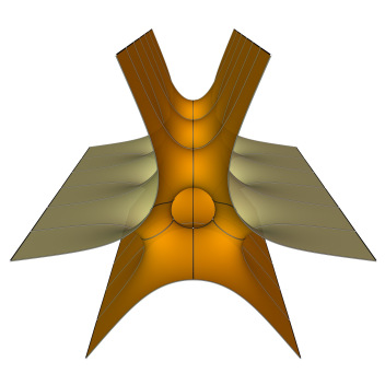
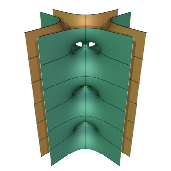
Figure 4. Karcher–Scherk saddle towers with handles.

Example 4 (Toroidal saddle towers).

Figure 4 shows symmetric Karcher–Scherk saddle towers with a vertical tunnel in the middle. They were first constructed by Karcher [Kar88] with explicit Weierstrass data defined on tori, hence the name. In the framework of our construction, the one with 6 ends arises from three lines forming an equiangular triangle, the one with 8 ends arises from four lines forming a square.

Note that the one with 8 ends has parallel ends, but they do not correspond to the parallel rays in the graph. In fact, we have $\xi(\varepsilon)\equiv 0$ and the Scherk ends bend from vertical and horizontal directions in the limit $\varepsilon\to 0$ all the way to the diagonal directions as $\varepsilon$ increases, forming new parallel pairs. If $\varepsilon$ increase further, the Scherk ends will intersect. ∎

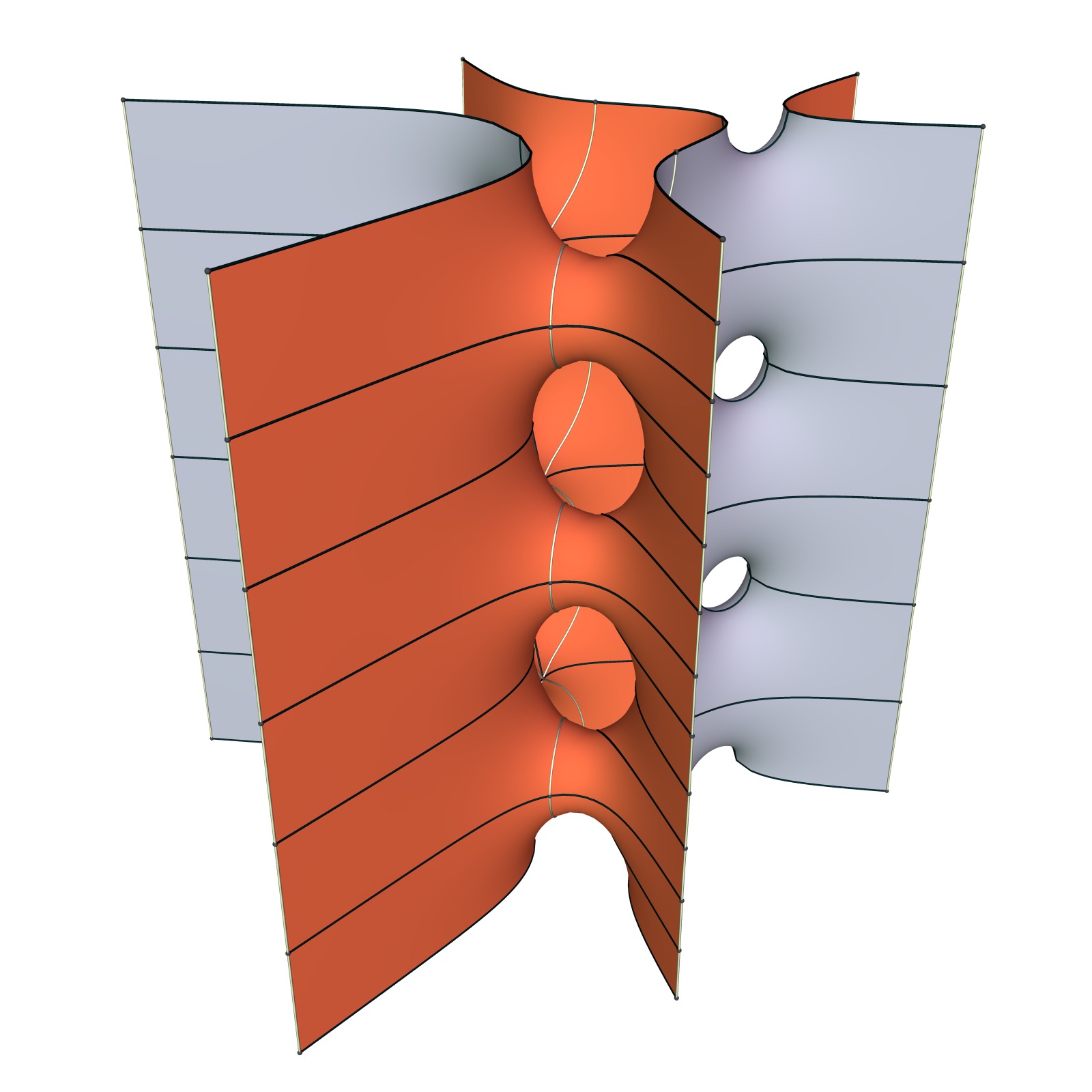
Figure 5. The Costa–Scherk surfaces.

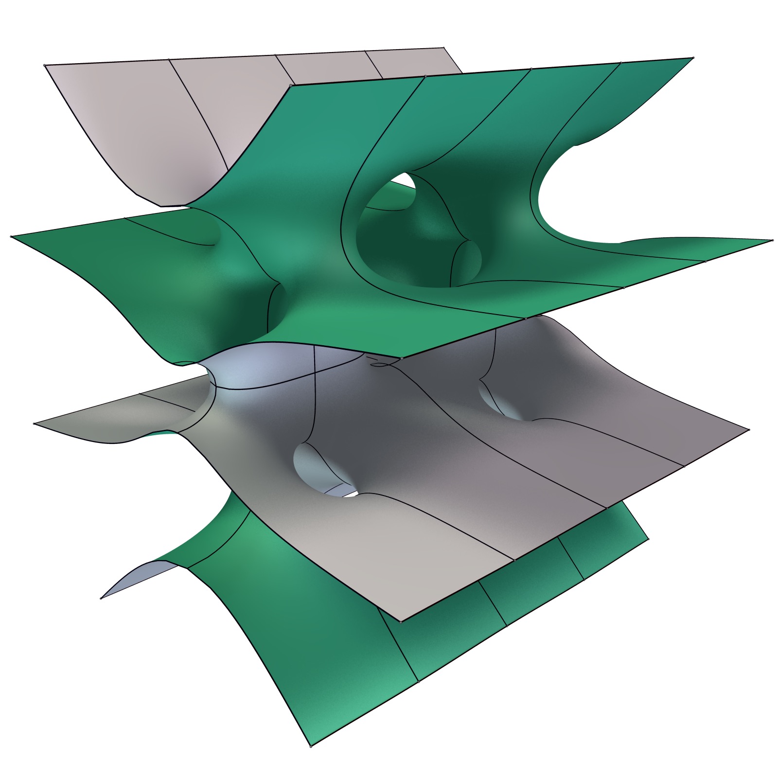
Figure 6. The da Silva–Batista surface.

Example 5 (Costa–Scherk surfaces).

In Figure 5 is a family that arises again from three lines forming an equiangular triangle. But this time we use a different trivial phase function. The SPMSs looks like a tower of Costa surfaces, hence the name. ∎

Example 6 (Da Silva–Batista surfaces).

In Figure 6 is a family that arises from an arrangement of four lines. As we have 8 ends, the family is described by 5 parameters up to scalings and Euclidean motions. In particular, it includes the saddle tower limit of the 2-parameter family constructed in [dSRB10], for which vertical reflection planes were assumed. ∎

3.3. Singly periodic gyroids

Example 7 (Singly periodic rGL).

In view of Lemma 3, a SPMS with Scherk ends and no horizontal symmetry plane must arise from a graph with a cycle of length at least three. The configuration on the left of Figure 7, where three lines form an equiangular triangle, is therefore the smallest non-symmetric, balanced, and rigid example. It can be seen as the singly periodic analogue of the rGL family of triply periodic minimal surfaces; see [Che21] and [CT21]. Note that, if the triangle was not equiangular, then the only possible balanced phase functions are the trivial ones, and we obtain a deformation of the toroial saddle tower with 6 ends (see Example 4). One sees here that the vertical balance does not depend continuously on the graph; see Remark 7. ∎

Example 8 (Singly periodic tG, inconclusive).

In the same spirit, the configuration on the right of Figure 7, where four lines form a square, can be seen as the singly periodic analogue of the tG family of triply periodic minimal surfaces; see [Che21] and [CT21]. This configuration is balanced, but not vertically rigid: It seems that one may vertically slide two non-adjacent saddle towers with respect to the others without any horizontal deformation of the graph. Hence our construction is not conclusive on this configuration. Even if this configuration does give rise to SPMSs with Scherk ends, it would still be challenging to determine their embeddedness, as Theorem 6 does not apply here. ∎

Figure 7. Singly periodic analogues of rGL and tG surfaces.

3.4. Miscellaneous examples

Example 9 (Polygrams).

Non-symmetric examples can be produced from the graph that appears as a simple arrangement of $k$ lines, $k>4$, that form a regular polygram. More specifically, such a graph contains a clockwise cycle whose edges are all of the shortest length. We choose $\phi^{\circ}$ that takes the same value on all half-edges in this cycle, and its value on other half-edges can be determined (not necessarily unique!) by solving the period and balance problems. Figure 8 shows two examples with $k=5$ and $k=8$. These configurations all appear as line arrangements. If $k$ is odd, the embeddedness follows from Theorem 3. If $k$ is even, and $\xi(\varepsilon)\equiv 0$, the embeddedness can be determined by Theorem 6. ∎

Figure 8. Non-symmetric examples from polygrams.

Example 10.

Figure 9 shows a graph with two vertices of degree 4 and one vertex of degree 6. Let $c$ be the unique counterclockwise cycle in the graph. Using the explicit values of $\mu_{h}$ computed in [CT21], one verifies that $P^{\text{hor}}_{c}(\mu^{a})=0$. So we have, very conveniently, $\dot{\zeta}=0$ and $\dot{\chi}^{\circ}=\xi^{\circ}\in\mathcal{D}$.

Label four rays as shown in the Figure. One verifies that $\xi=(\dot{x},\dot{\vartheta})$ with $\dot{x}=0$,

$$2\dot{\theta}_{1}=-\dot{\theta}_{2}=\dot{\theta}_{3}=-2\dot{\theta}_{4}>0,$$

and $\dot{\theta}_{r}=0$ for other rays, is a vector in $\mathcal{D}$. This deformation is illustrated by dashed lines in the figure. If we choose this deformation as $\xi^{\circ}$, then the Scherk ends corresponding to rays $1$ and $4$ bend away from the parallel Scherk ends, and the embeddedness follows from Theorem 4. ∎

Figure 9. An infinitesimal deformation $\xi^{\circ}$ that resolve parallel Scherk ends.

Example 11 (Benzene, inconclusive).

It is tempting to construct SPMSs from the Benzene-like graph in Figure 10 with $12$ rays. However, Mathematica reports that the space $\mathcal{D}$ of balance-preserving deformations is of dimension $11>12-2$, so the graph is not rigid. To explicitly count the dimension of $\mathcal{D}$, note that rotation contributes one dimension. Up to rotation, all the infinitesimal deformations in $\mathcal{D}$ must preserve the directions of closed edges; such deformations for the hexagon contribute four dimensions (including the scaling). Finally, the deformations that open up parallel rays also preserve the balance to the first order; they contribute six dimensions, one for each pair. Our main theorem is therefore inconclusive here. ∎

Figure 10. This graph is not rigid.

4. Construction

This section is dedicated to the proof of Theorem 2 and the embeddedness statements. As we have explained, the construction of the SPMSs will only be sketched. The readers are referred to the first paper of this series [CT21] for omitted technical details. Only the embeddedness Theorem 6 will receive an elaborated proof in Section 4.4.4 because it is our major technical concern, and the involved argument was not detailed before.

4.1. Weierstrass parameterization

We construct a conformal minimal immersion using the Weierstrass parameterization

$$\Sigma\ni z\mapsto\operatorname{Re}\int^{z}(\Phi_{1},\Phi_{2},\Phi_{3}),$$

where $\Sigma$ is a Riemann sphere and $\Phi_{i}$ are meromorphic 1-forms on $\Sigma$ satisfying the conformality equation

(4) $$Q=\Phi_{1}^{2}+\Phi_{2}^{2}+\Phi_{3}^{2}=0.$$

4.1.1. Riemann surface

To each vertex $v\in\mathsf{V}$, we associate a Riemann sphere $\hat{\mathbb{C}}_{v}$. To each half-edge $\eta\in v$, we associate a complex number $p^{\circ}_{\eta}\in\hat{\mathbb{C}}_{v}$, so that $\hat{\mathbb{C}}_{v}$ punctured at $p^{\circ}_{\eta}$ provides a conformal model for the saddle tower $\mathscr{S}_{v}$. Then for every $h\in\mathsf{H}\setminus\mathsf{R}$, we identify $p^{\circ}_{h}$ and $p^{\circ}_{-h}$. The resulting singular Riemann surface with nodes is denoted $\Sigma_{0}$.

As $\varepsilon$ increases, we open nodes into necks in the standard way:

For each $\eta\in\mathsf{H}$, let $p_{\eta}\in\hat{\mathbb{C}}_{v(\eta)}$ be a complex parameter in the neighborhood of $p^{\circ}_{\eta}$, and consider an adapted local coordinate $w_{h}$ in a neighborhood of $p_{\eta}\in\hat{\mathbb{C}}_{v(\eta)}$ such that $w_{\eta}(p_{\eta})=0$. Since the graph is finite, it is possible to fix a small number $\delta>0$ independent of $v$ such that, for $p$ sufficiently close to $p^{\circ}$, the disks $|w_{\eta}|<2\delta$ are disjoint.

In the neighborhood of $0$, consider $t=(t_{h})_{h\in\mathsf{H}\setminus\mathsf{R}}$ that is symmetric in the sense that $t_{h}=t_{-h}$. Then for every $h\in\mathsf{H}\setminus\mathsf{R}$, we remove the disk

$$|w_{h}|<|t_{h}|/\delta,$$

and identify the annuli

$$|t_{h}|/\delta\leq|w_{h}|\leq\delta\quad\text{and}\quad|t_{-h}|/\delta\leq|w_{-h}|\leq\delta$$

by

$$w_{h}w_{-h}=t_{h}.$$

This produces a Riemann surface, possibly with nodes, denoted by $\Sigma_{t}$, depending on the parameters $t$ and $p$.

4.1.2. Weierstrass data

Let $A_{h}$ denote the counterclockwise circle $|w_{h}|=\delta$. We need to solve the A-period problem

$$\operatorname{Re}\int_{A_{\eta}}(\Phi_{1},\Phi_{2},\Phi_{3})=(0,0,2\pi\sigma_{\eta}),\quad\forall\eta\in\mathsf{H}.$$

For this purpose, we define $\Phi_{1}$, $\Phi_{2}$, and $\Phi_{3}$ as the unique regular 1-forms on $\Sigma_{t}$ with simple poles at $p_{r}$, $r\in\mathsf{R}$, possibly also at $\infty_{v}$, $v\in\mathsf{V}$, and the A-periods

$$\int_{A_{\eta}}(\Phi_{1},\Phi_{2},\Phi_{3})=2\pi{\rm i}(\alpha_{\eta},\beta_{\eta},\gamma_{\eta}-{\rm i}\sigma_{\eta}),\quad\forall\eta\in\mathsf{H},$$

where $(\alpha,\beta,\gamma)\in(\mathcal{A}\times\mathcal{R})^{3}$. Then the A-period problems are solved by definition. We choose the following central value for the parameters:

$$\alpha^{\circ}_{\eta}=-\cos(\theta^{\circ}_{\eta}),\qquad\beta^{\circ}_{\eta}=-\sin(\theta^{\circ}_{\eta}),\qquad\gamma^{\circ}_{\eta}=0.$$

Then at $\varepsilon=0$ and the central values of all parameters, $(\Phi^{\circ}_{1},\Phi^{\circ}_{2},\Phi^{\circ}_{3})$ is precisely the Weierstrass data of the saddle tower $\mathscr{S}_{v}$.

4.1.3. Balance and period problems

We want $\infty_{v}$ to be regular points for all $v\in\mathsf{V}$. For this purpose, we need to solve the balance equations

(5) $$F_{v}(\alpha,\beta,\gamma)=\sum_{\eta\in v}(\alpha_{\eta},\beta_{\eta},\gamma_{\eta})=0,\qquad\text{for all }v\in\mathsf{V}.$$

A half-edge $r\in\mathsf{R}$ corresponds to a Scherk end asymptotic to a vertical plane. So we require that

(6) $$\gamma_{r}\equiv 0\quad\text{and}\quad|\alpha_{r}+{\rm i}\beta_{r}|=\alpha_{r}^{2}+\beta_{r}^{2}\equiv 1$$

no matter the value of other parameters. This guarantees that (the stereographic projection of) the Gauss map $G=-(\Phi_{1}+{\rm i}\Phi_{2})/\Phi_{3}$ extends holomorphically to the punctures $p_{r}$ with unitary values.

Recall from [CT21] that, for every vertex $v$, we fix an origin $O_{v}\in\mathbb{C}_{v}$ bounded away from all punctures $p_{h}$, and a path $B_{h}$ from $O_{v(h)}$ to $O_{v(-h)}$ through the neck corresponding to $h$; see [CT21] for the rigorous descriptions. Then for a cycle $c=(h_{1},\cdots,h_{n})$, we define $B_{c}$ as the concatenation $B_{h_{1}}*\cdots*B_{h_{n}}$. For each $c\in\mathsf{F}$, we need to solve the following B-period problems

(7) $$\operatorname{Re}\int_{B_{c}}(\Phi_{1},\Phi_{2},\Phi_{3})=0.$$

4.2. Using the Implicit Function Theorem

4.2.1. Solving conformality problems

At $\varepsilon=0$ and the central value of all parameters, $\Phi^{\circ}_{1}$ has $\deg(v)-2$ zeros denoted $z^{\circ}_{v,j}$ for $1\leq j\leq\deg(v)-2$. We may assume that these zeros are simple and not at $\infty_{v}$. When the parameters are close to their central values, $\Phi_{1}$ has a simple zero $z_{v,j}$ close to $z^{\circ}_{v,j}$ in $\hat{\mathbb{C}}_{v}$. The same argument as in [CT21] proves that the conformality condition (4) is satisfied if (5) and the following equations are solved:

(8) $$\int_{A_{\eta}}\frac{Q}{\Phi_{1}} =0, \eta\in\mathsf{H},$$

(9) $$\operatorname{Res}\left(\frac{Q}{\Phi_{1}},z_{v,j}\right) =0, 1\leq j\leq\deg(v)-3,\;v\in\mathsf{V}.$$

We make the change of parameters

$$\alpha_{\eta}+{\rm i}\beta_{\eta}=-\rho_{\eta}\exp({\rm i}\theta_{\eta})$$

for $\eta\in\mathsf{H}$. The central value of $\theta_{\eta}$ is $\theta^{\circ}_{\eta}$ given by the graph. Recall that we write $\theta=(\theta_{\eta})_{\eta\in\mathsf{H}}$.

Proposition 4.

For $(t,\theta)$ in a neighborhood of $(0,\theta^{\circ})$, there exist unique values for $p_{\eta}$, $\rho_{\eta}$, and $\gamma_{\eta}$, depending real-analytically on $(t,\theta)$, such that the equations (8) and (9) are solved under the condition (6). At $\varepsilon=0$ and the central values of the parameters, we have

$$p_{\eta}=p^{\circ}_{\eta},\quad\rho_{\eta}=1,\quad\gamma_{\eta}=0$$

for $\eta\in\mathsf{H}$ no matter the values of other parameters. Moreover, at $(t,\theta)=(0,\theta^{\circ})$, we have the Wirtinger derivatives

(10) $$\frac{\partial\rho_{h}}{\partial t_{h}}=-\frac{1}{2}\Upsilon_{h}\Upsilon_{-h}\quad\text{and}\quad\frac{\partial\gamma_{h}}{\partial t_{h}}=-\frac{{\rm i}}{2}\sigma_{h}\Upsilon_{h}\Upsilon_{-h}$$

for each $h\in\mathsf{H}\setminus\mathsf{R}$.

The proof in [CT21] applies here almost word for word, so we omit the proof. From now on, we assume that $p$, $\rho$ and $\gamma$ are given by Proposition 4.

4.2.2. Solving horizontal balance and period problems

For $h\in\mathsf{H}\setminus\mathsf{R}$, we make the change of parameters

$$t_{h}=-\exp\Big{(}-\ell_{h}\varepsilon^{-2}-{\rm i}\sigma_{h}\phi_{h}\Big{)}.$$

Note that $t_{h}$ is a flat function in $\varepsilon$ in the sense that all derivatives of $t_{h}$ in $\varepsilon$ vanish. The central value of $\ell_{h}$ is $\ell^{\circ}_{h}$, the length of the segment $\varrho(e(h))$. The central value of $\phi_{h}$ is the prescribed phase function $\phi^{\circ}_{h}$. We combine $\ell$ and $\theta$ into

$$x_{h}=\ell_{h}e^{{\rm i}\theta_{h}},$$

whose central value is $x^{\circ}_{h}$ as given by the graph. Recall that we write $\vartheta=(\theta_{r})_{r\in\mathsf{R}}$, and $\chi=(x,\vartheta)$. For $\chi$ in an neighborhood of $\chi^{\circ}$, we change to the variable

$$\chi=\chi^{\circ}+\varepsilon^{2}\xi+\zeta$$

where $\xi\in\mathcal{D}$ and $\zeta\in\mathcal{D}^{\perp}$.

Proposition 5.

Assume that the graph $\Gamma$ is balanced and rigid. For $(\varepsilon,\xi,\phi)$ in a neighborhood of $(0,\xi^{\circ},\phi^{\circ})$, there exist unique values for $\zeta$, depending smoothly on $(\varepsilon,\xi,\phi)$, such that the horizontal components of the balance equations (5) and the B-period equations (7) are solved. Moreover, $\zeta$ is an even function of $\varepsilon$ and, at $\varepsilon=0$, we have $\zeta(0,\xi,\phi)=0$ and $\dfrac{1}{2}\dfrac{\partial^{2}\zeta}{d\varepsilon^{2}}(0,\xi,\phi)=\dot{\zeta}$ is the unique solution to (1) in $\mathcal{D}^{\perp}$ no matter the values of $\xi$ and $\phi$.

The proof in [CT21] applies here with some modification. We sketch a proof here because some computations will be useful later for the embeddedness proofs.

Sketched proof.

Define for $(\varepsilon,\xi,\phi)$ in a neighborhood of $(0,\xi^{\circ},\phi^{\circ})$ and $h\in\mathsf{H}\setminus\mathsf{R}$

$$\mathcal{P}^{\text{hor}}_{h}(\varepsilon,\xi,\phi)=\varepsilon^{2}\Big{(}\operatorname{Re}\int_{B_{h}}\Phi_{1}+{\rm i}\operatorname{Re}\int_{B_{h}}\Phi_{2}\Big{)},$$

for $c\in\mathsf{F}$

$$\mathcal{P}^{\text{hor}}_{c}(\varepsilon,\xi,\phi)=\varepsilon^{2}\Big{(}\operatorname{Re}\int_{B_{c}}\Phi_{1}+{\rm i}\operatorname{Re}\int_{B_{c}}\Phi_{2}\Big{)}=\sum_{h\in c}\mathcal{P}^{\text{hor}}_{h}(\varepsilon,\xi,\phi),$$

and for $v\in\mathsf{V}$

(11) $$\mathcal{F}^{\text{hor}}_{v}(\varepsilon,\xi,\phi)=-\operatorname{div}_{v}(\alpha+{\rm i}\beta)=\sum_{h\in v}\rho_{h}e^{{\rm i}\theta_{h}}.$$

In [CT21] we have computed that

(12) $$\mathcal{P}^{\text{hor}}_{h}(\varepsilon,\xi,\phi)=\rho_{h}x_{h}+\varepsilon^{2}\lambda_{h}(\varepsilon,\xi,\phi)$$

where $\lambda_{h}$ is analytic in $t_{h}$ and $\lambda_{h}(0,\xi,\phi)=\mu_{h}-\mu_{-h}=:\mu^{a}_{h}$ no matter the values of $\xi$ and $\phi$. So $\lambda_{h}$ is flat in $\varepsilon$. We have also computed that

(13) $$\begin{cases}\mathcal{P}^{\text{hor}}(\varepsilon,\xi,\phi)=P^{\text{hor}}(\chi)+\varepsilon^{2}P^{\text{hor}}(\mu^{a})+\text{flat terms},\\ \mathcal{F}^{\text{hor}}(\varepsilon,\xi,\phi)=F^{\text{hor}}(\chi)+\text{flat terms}.\end{cases}$$

Write $\mathcal{F}^{\text{hor}}=(\mathcal{F}^{\text{hor}}_{v})_{v\in\mathsf{V}}$ and $\mathcal{P}^{\text{hor}}=(\mathcal{P}^{\text{hor}}_{c})_{c\in\mathsf{F}}$. We want to solve

(14) $$(\mathcal{F}^{\text{hor}},\mathcal{P}^{\text{hor}})(\varepsilon,\xi,\phi)=0.$$

If $\Gamma$ is balanced, the system is solved at $\varepsilon=0$ with $\zeta=0$ no matter the values of $\xi$ and $\phi$. If $\Gamma$ is rigid, then by the Implicit Function Theorem, the system has a unique solution $\zeta(\varepsilon,\xi,\phi)$, depending smoothly on $(\varepsilon,\xi,\phi)$ in a neighborhood of $(0,\xi^{\circ},\phi^{\circ})$.

The system (14) is even in $\varepsilon$, so must be the solution $\zeta$. Taking the second derivative of (14) with respect to $\varepsilon$ at $\varepsilon=0$ gives the linear system

$$\begin{dcases}2P^{\text{hor}}_{c}(\mu^{a})+P^{\text{hor}}_{c}\Big{(}\frac{\partial^{2}\zeta}{\partial\varepsilon^{2}}\Big{)}=0,&c\in\mathsf{F},\\ DF^{\text{hor}}_{v}(\chi^{\circ})\cdot\Big{(}\frac{\partial^{2}\zeta}{\partial\varepsilon^{2}}\Big{)}=0,&v\in\mathsf{V},\end{dcases}$$

which proves that $\dfrac{1}{2}\dfrac{\partial^{2}\zeta}{\partial\varepsilon^{2}}$ must be the unique solution $\dot{\zeta}\in\mathcal{D}^{\perp}$ to the linear system (1) in $\mathcal{D}^{\perp}$. ∎

4.2.3. Solving vertical balance and period problems

Proposition 6.

Assume that the phase function $\phi^{\circ}$ is balanced and rigid with respect to the prescribed deformation $\xi^{\circ}\in\mathcal{D}$. For $(\varepsilon,\xi)$ in a neighborhood of $(0,\xi^{\circ})$, there exist unique values for $(\phi_{h})_{h\in\mathsf{H}\setminus\mathsf{R}}$, depending smoothly on $\varepsilon$ and $\xi$, such that $\phi_{h}(0,\xi^{\circ})=\phi^{\circ}_{h}$, and the vertical components of the balance equations (5) and the B-period equations (7) are solved.

The proof in [CT21] applies here with only slight modification, but we still sketch a proof for completeness.

Sketched proof.

Define for $(\varepsilon,\xi)$ in a neighborhood of $(0,\xi^{\circ})$ and $c\in\mathsf{F}$

$$\mathcal{P}^{\text{ver}}_{c}(\varepsilon,\xi,\phi)=\operatorname{Re}\int_{B_{c}}\Phi_{3},$$

and for $\varepsilon>0$ and $b\in\mathsf{B}_{m}^{*}$,

$$\mathcal{F}^{\text{ver}}_{b}(\varepsilon,\phi):=-\exp(\ell^{\circ}_{b}\varepsilon^{-2})\operatorname{div}_{b}(\gamma(\varepsilon,\xi,\phi)).$$

By the same computation as in [CT21], we have

$$\mathcal{P}^{\text{ver}}_{c}(0,\xi,\phi)=P^{\text{ver}}_{c}(\phi)\pmod{2\pi}$$

no matter the value of $\xi$, and that $\mathcal{F}^{\text{ver}}_{b}$ extends smoothly at $\varepsilon=0$ to

$$\mathcal{F}^{\text{ver}}_{b}(0,\xi,\phi)=\sum_{h\in m(b)}\Upsilon_{h}\Upsilon_{-h}\sin(\phi_{h})\exp\left(-\operatorname{Re}({\dot{x}}_{h}\exp(-{\rm i}\theta^{\circ}_{h}))\right),$$

where $\xi+\dot{\zeta}=(\dot{x},\dot{\vartheta})$. In particular,

$$\mathcal{F}^{\text{ver}}_{b}(0,\xi^{\circ},\phi)=F^{\text{ver}}_{b}(\phi).$$

Write $\mathcal{F}^{\text{ver}}=(\mathcal{F}^{\text{ver}}_{b})_{b\in\mathsf{B}_{m}^{*}}$ and $\mathcal{P}^{\text{ver}}=(\mathcal{P}^{\text{ver}}_{c})_{c\in\mathsf{F}}$. We want to solve

$$(\mathcal{F}^{\text{ver}},\mathcal{P}^{\text{ver}})(\varepsilon,\xi,\phi)=0.$$

If the phase function $\phi^{\circ}$ is balanced with respect to $\xi^{\circ}$, the system is solved at $(\varepsilon,\xi)=(0,\xi^{\circ})$ by $\phi=\phi^{\circ}$. If $\phi^{\circ}$ is rigid, then by the Implicit Function Theorem, the system has a unique solution $\phi(\varepsilon,\xi)$, depending smoothly on $(\varepsilon,\xi)$ in a neighborhood of $(0,\xi^{\circ})$, such that $\phi(0,\xi^{\circ})=\phi^{\circ}$. ∎

The same argument as in [CT21] shows that the immersion is regular. This finishes the proof of Theorem 2.

4.3. Symmetric SPMSs

A trivial phase function is trivially balanced, but not necessarily rigid. So Theorem 1 is not contained in our main Theorem 2. But its proof is very similar, only much easier, hence we only give a brief sketch here. The readers are referred to [You09] and [Tra01] for technical details.

The reflection in the horizontal symmetry plane correspond to an involution $\rho$ of $\Sigma_{t}$ that restricts to $\rho(z)=\overline{z}$ on $\hat{\mathbb{C}}_{v}$ for every vertex $v$. We restrict to the parameters $p_{h}$ to real values, and set $\gamma\equiv 0$ so that the vertical balance problem is trivially solved. This ensures that $\rho^{*}\Phi_{1,2}=\overline{\Phi}_{1,2}$ and $\rho^{*}\Phi_{3}=-\overline{\Phi}_{3}$, so the surface carries the desired symmetry; see [You09].

Since $\phi\equiv\phi^{\circ}$ is trivial, we have $t_{h}\in\mathbb{R}$, negative if $\phi_{h}=0$, positive if $\phi_{h}=\pi$. For each $c\in\mathsf{F}$, we choose the integral path $B_{c}$ as the concatenation of $B^{\prime}_{h}$ where

• if $\phi_{h}=0$, $B^{\prime}_{h}$ consists of the real segment $w_{h}=-t_{h}/\delta>0$ to $w_{\varsigma(h)}=-\delta<0$.

• if $\phi_{h}=\pi$, $B^{\prime}_{h}$ consists of an clockwise half-circle around $p_{h}$ from $w_{h}=-t_{h}/\delta<0$ to $w_{h}=t_{h}/\delta>0$, followed by the real segment to $w_{\varsigma(h)}=-\delta$.

This careful choice of path makes it convenient to compute that $\operatorname{Re}\int_{B_{c}}\Phi_{3}=0\pmod{2\pi}$; see [You09]. So the vertical period problem is automatically solved.

We then use the Implicit Function Theorem to solve the conformality problem and horizontal balance and period problems, as we did above for the general case. The result is a continuous family of symmetric SPMSs depending on $|\mathsf{R}|-1$ parameters. One of them is $\varepsilon$. The other parameters correspond to the deformations $\chi\in\mathcal{M}$; cf. [Tra01]. This finished the construction of symmetric SPMSs.

4.4. Embeddedness

We now prove the scenarios where the surfaces $M_{\varepsilon,\xi}$ in Theorem 2 are embedded, at least for some $(\varepsilon,\xi)$ in a neighborhood of $(0,\xi^{\circ})$. In fact, the same proof as in [CT21] proves the embeddedness except for the Scherk ends. It also proves the embeddedness of each Scherk end. The only problem is that the Scherk ends might intersect each other. We then omit this part of the proof, and focus on the bendings of the Scherk ends.

4.4.1. The safe case

If the graph has no parallel rays, then the Scherk ends would not intersect for $(\varepsilon,\xi)$ sufficiently close to $(0,\xi^{\circ})$. This proves the scenario in Theorem 3, and has been considered in [Tra01].

4.4.2. Lowest-order bending

Otherwise, we must analyse how the Scherk ends bend. For this purpose, let us consider a 1-parameter family $M_{\varepsilon,\xi(\varepsilon)}$ where $\xi(\varepsilon)\in\mathcal{D}$ is a fixed analytic function such that $\xi(0)=\xi^{\circ}$. All other parameters have been solved as a smooth function of $\varepsilon$. Write

$$\zeta(\varepsilon)=\widetilde{\zeta}(\varepsilon)+\overline{\zeta}(\varepsilon).$$

Here and in the remaining of the paper, for any smooth function $f(x)$, we use $\widetilde{f}(x)$ to denote the analytic function given by the Taylor series of $f$ in $x$, and use $\overline{f}(x)$ to denote the non-analytic remainder.

By Proposition 5, the first term of $\widetilde{\zeta}(\varepsilon)$ is $\varepsilon^{2}\dot{\zeta}$. Hence the lowest-order deformation of the graph is $\dot{\chi}^{\circ}=\xi^{\circ}+\dot{\zeta}$. If the parallel Scherk ends bend away from each other under this deformation, the Scherk ends would not intersect for $(\varepsilon,\xi)$ sufficiently close to $(0,\xi^{\circ})$. This proves the scenario in Theorem 4.

4.4.3. Analytic bending

If the lowest-order deformation does not help, we may look into higher order deformations, and eventually use the entire Taylor series. In view of (13), $\widetilde{\zeta}(\varepsilon)\in\mathcal{D}^{\perp}$ solves the non-linear system

$$\begin{cases}\widetilde{\mathcal{P}^{\text{hor}}_{c}}=P^{\text{hor}}_{c}(\widetilde{\zeta})+\varepsilon^{2}P^{\text{hor}}_{c}(\mu^{a}_{h})=0,&c\in\mathsf{F},\\ \widetilde{\mathcal{F}^{\text{hor}}_{v}}=F^{\text{hor}}_{v}(\widetilde{\chi})=0,&v\in\mathsf{V},\end{cases}$$

where $\widetilde{\chi}=\chi^{\circ}+\varepsilon^{2}\xi(\varepsilon)+\widetilde{\zeta}(\varepsilon)$. This is exactly the system (2). Moreover, since the graph is balanced and rigid, there is a unique solution $\widetilde{\zeta}(\varepsilon)$ for $\varepsilon$ sufficiently small. If the parallel Scherk ends bend away from each other under the deformation $\widetilde{\chi}(\varepsilon)$ for sufficiently small $\varepsilon$, then the Scherk ends would not intersect for sufficiently small $\varepsilon$. This proves the scenario described in Theorem 5.

4.4.4. Non-analytic bending

The remaining of the paper is dedicated to the proof of Theorem 6. This is the only part of the paper that contains detailed arguments, because the technical details here were never written down before.

Interestingly, if the graph appears as a simple line arrangement, the analytic part $\widetilde{\chi}(\varepsilon)$ does not resolve parallel Scherk ends no matter how many terms are used. This follows from the following lemma.

Lemma 7.

Write $\widetilde{\chi}(\varepsilon)=(\widetilde{x}(\varepsilon),\widetilde{\vartheta}(\varepsilon))$. If the graph appears as a simple line arrangement, then we have $\widetilde{\theta}_{r}=\widetilde{\theta}_{r^{\prime}}+\pi\pmod{2\pi}$ whenever the rays $r$ and $r^{\prime}$ belong to the same line.

Proof.

Explicitly, we have the Taylor series

$$\widetilde{\mathcal{F}^{\text{hor}}_{v}}=F^{\text{hor}}_{v}(\widetilde{\chi})=-\sum_{\eta\in v}e^{{\rm i}\widetilde{\theta}_{\eta}}.$$

Since the graph appears as a simple line arrangement, every vertex is of degree four. Consequently, $\widetilde{\mathcal{F}^{\text{hor}}}=0$ if and only if

$$\widetilde{\theta}_{\varsigma^{2}(\eta)}=\widetilde{\theta}_{\eta}+\pi\pmod{2\pi}.$$

So, if two Scherk ends correspond to rays from the same line, their directions $\widetilde{\theta}$ must remain opposite. ∎

Now assume that the line arrangement contains a pair of parallel rays. If they bend away from each other under the deformation $\widetilde{\chi}$, then by the Lemma, the other rays on the same lines must bend towards each other, creating an unwanted intersection. The only way to avoid this is to let the parallel rays remain parallel under the deformations $\widetilde{\chi}$, i.e. $\widetilde{\theta}_{r}(\varepsilon)=\widetilde{\theta}_{r+1}(\varepsilon)$ for sufficiently small $\varepsilon$ whenever $\theta^{\circ}_{r}=\theta^{\circ}_{r+1}$. This is assumed in Theorem 6.

Remark 11.

There are certainly other situations that $\widetilde{\chi}$ can not resolve parallel Scherk ends; see Example 3. But we have no plan to classify all such situations.

Then we proceed to investigate the non-analytic part $\overline{\zeta}(\varepsilon)$. Let $\ell^{\circ}_{\min}$ be the length of the shortest edges in the graph, and write $\tau(\varepsilon)=\exp(-\ell^{\circ}_{\min}/\varepsilon^{2})$. Recall that $m(\mathsf{H})=\{h\in\mathsf{H}\setminus\mathsf{R}\colon\ell^{\circ}_{h}=\ell^{\circ}_{\min}\}$.

Proposition 8.

$$\overline{\zeta}\sim\widehat{\zeta}\tau$$

where $\widehat{\zeta}$ is the unique solution in $\mathcal{D}^{\perp}$ to (3).

Proof.

We first prove that $\overline{\zeta}\in O(\tau)$. Assume instead that $\overline{\zeta}\sim\kappa f(\varepsilon)$ for some $\kappa\in\mathcal{D}^{\perp}$ and $f(\varepsilon)\in\omega(\tau(\varepsilon))$ ($f$ dominates $\tau$) as $\varepsilon\to 0$. In [CT21], we have computed from (10) that

$$\overline{\gamma}_{h}\sim-K_{h}\sin\phi^{\circ}_{h}e^{-\ell^{\circ}_{h}/\varepsilon^{2}}.$$

A similar computation yields

$$\overline{\rho}_{h}\sim K_{h}\cos\phi^{\circ}_{h}e^{-\ell^{\circ}_{h}/\varepsilon^{2}}.$$

Moreover, we have seen that $\lambda_{h}(\varepsilon)$ is analytic in $t_{h}$, so $\overline{\lambda}_{h}\in O(e^{-\ell^{\circ}_{h}/\varepsilon^{2}})$. As $\ell^{\circ}_{h}\geq\ell^{\circ}_{\min}$, the functions $\overline{\rho}$ and $\overline{\lambda}$ are all in $O(\tau)$, hence all dominated by $f$ as $\varepsilon\to 0$. Then a routine computation from (11) and (12) yields, as $\varepsilon\to 0$, that

$$\begin{cases}f(\varepsilon)^{-1}\overline{\mathcal{P}^{\text{hor}}}(\varepsilon)\to P^{\text{hor}}_{c}(\kappa)=0,&c\in\mathsf{F},\\ f(\varepsilon)^{-1}\overline{\mathcal{F}^{\text{hor}}}(\varepsilon)\to DF^{\text{hor}}_{v}(\chi^{\circ})\cdot\kappa=0,&v\in\mathsf{V},\end{cases}$$

hence $\kappa=0$.

Then we compute the coefficient $\widehat{\zeta}\in\mathcal{D}^{\perp}$ of $\tau$. Note that $\overline{\rho}_{h}\in o(\tau)$ as $\varepsilon\to 0$ if and only if $\ell^{\circ}_{h}>\ell^{\circ}_{\min}$, i.e. $h\not\in m(\mathsf{H})$. Using this fact, a routine computation from (11) and (12) yields, as $\varepsilon\to 0$, that

$$\begin{dcases}\tau(\varepsilon)^{-1}\overline{\mathcal{P}^{\text{hor}}}(\varepsilon)\to P^{\text{hor}}_{c}(\widehat{\zeta})+\sum_{h\in c\cap m(\mathsf{H})}x_{h}K_{h}\cos\phi^{\circ}_{h}=0,&c\in\mathsf{F},\\ \tau(\varepsilon)^{-1}\overline{\mathcal{F}^{\text{hor}}}(\varepsilon)\to DF^{\text{hor}}_{v}(\chi^{\circ})\cdot\widehat{\zeta}+\sum_{h\in v\cap m(\mathsf{H})}u_{h}K_{h}\cos\phi^{\circ}_{h}=0,&v\in\mathsf{V},\end{dcases}$$

so $\widehat{\zeta}$ must be the unique solution in $\mathcal{D}^{\perp}$ to (3).

Finally, we prove that $\widehat{\zeta}\neq 0$. This follows from the existence of a vertex $v$ such that the summation

(15) $$\sum_{h\in v\cap m(\mathsf{H})}u_{h}K_{h}\cos\phi_{h}$$

is not zero.

Assume the opposite, i.e. that the summation vanishes for every vertex. Define

$$V_{m}=\{v\in V\colon\exists h\in v\,\text{such that}\,\ell^{\circ}_{h}=\ell^{\circ}_{\min}\,\text{and}\,K_{h}\cos\phi^{\circ}_{h}\neq 0\}.$$

Clearly, if $V_{m}$ is not empty, it must contain at least two vertices. Note that $v\cap m(\mathsf{H})=m(v)$ if $v\in V_{m}$.

Take the convex hull of $\{\varrho(v)\colon v\in V_{m}\}$, and consider an arbitrary vertex $v$ at a corner of the convex hull. Since every vertex is of degree four, $m(v)$ consists of either a single half-edge, or two half-edges whose corresponding unit vectors are linearly independent. In either case, the summation (15) vanishes if and only if $K_{h}\cos\phi^{\circ}_{h}=0$ for all $h\in m(v)$. This contradicts our assumption that $v\in V_{m}$.

So $V_{m}$ is empty, meaning that $K_{h}\cos\phi^{\circ}_{h}=0$ for all $h\in m(\mathsf{H})$. Recall from [CT21] that $K_{h}>0$, so $\cos\phi^{\circ}_{h}=0$ for all $h\in m(\mathsf{H})$. Recall that the vertical force along $h$ is $K_{h}\sin\phi^{\circ}_{h}$. So $K_{h}\cos\phi^{\circ}_{h}$ is nothing but the derivative of the vertical force with respect to $\phi_{h}$ at $\phi^{\circ}_{h}$. Hence for a cut $b\in\mathsf{B}_{m}$ such that $\ell^{\circ}_{b}=\ell^{\circ}_{\min}$, the derivative of $F^{\text{ver}}_{b}$ with respect to $\phi$ at $\phi^{\circ}$ is $0$. This contradicts the assumption of Theorem 2 that the phase function is rigid.

This finishes the proof that the summation (15) must be non-zero for some vertex. We then conclude that $\widehat{\zeta}\neq 0$. ∎

If the graph appears as a simple line arrangement, and the deformation $\widetilde{\chi}$ does not create any self-intersection, then parallel Scherk ends are resolved if they bend away from each other under the deformation $\widehat{\zeta}$. This finises the proof for Theorem 6.

Appendix A Rigidity for simple graphs

We now prove Proposition 1. For this purpose, let us restate [PT07, Lemma 5.1] in the following form.

Lemma 9.

Under the conditions of Proposition 1, let $v$ be an arbitrary vertex and $L$ be a straight line though $\rho(v)$ that does not contain the geometric representation of any edge adjacent to $v$, then each side of $L$ contains the geometric representations of at least two edges adjacent to $v$.

This lemma allows us to adapt the argument in [Tra01] that proves the rigidity when the graph appears as a line arrangement.

Sketched proof of Proposition 1.

Up to a rotation, we may assume that the vectors $x_{h}\in\mathbb{C}$, $h\in\mathsf{H}$, all have non-zero real-parts. As a consequence, the geometric representations of the vertices all have distinct real parts. We then order the vertices by the real parts of $\rho(v)$, and order the faces by their left-most vertices.

For each vertex $v\in\mathsf{V}$, we choose two half-edges in $v$ whose directions, say $\theta^{\circ}_{v,1}$ and $\theta^{\circ}_{v,2}$, point to the left side; their existence follows from the lemma above. Then $DF^{\text{hor}}$ restricted to the variables $\dot{\theta}_{v,1}$ and $\dot{\theta}_{v,2}$ is a real square matrix with $|\mathsf{V}|\times|\mathsf{V}|$ blocks of size $2\times 2$. All blocks above the diagonal are $0$. To see this, note that if $v^{\prime}<v$, then $F^{\text{hor}}_{v}$ is independent of the chosen half-edges in $v^{\prime}$. The diagonal blocks are invertible because the unit vectors $e^{{\rm i}\theta^{\circ}_{v,1}}$ and $e^{{\rm i}\theta^{\circ}_{v,2}}$ are linearly independent; see [Tra01]. This proves that $DF^{\text{hor}}$ is surjective.

For each face $c\in\mathsf{F}$, we choose two half-edges in $c$ whose edges are adjacent to the left-most vertex of $c$. Let $\ell^{\circ}_{c,1}$ and $\ell^{\circ}_{c,2}$ be their lengths. Then $DP^{\text{hor}}$ restricted to the variables $\dot{\ell}_{c,1}$ and $\dot{\ell}_{c,2}$ is a real square matrix with $|\mathsf{F}|\times|\mathsf{F}|$ blocks of size $2\times 2$. All blocks above the diagonal are $0$. To see this, note that if $c^{\prime}<c$, then $P^{\text{hor}}_{c}$ is independent of chosen half-edges in $c^{\prime}$. The diagonal blocks are invertible because the unit vectors $e^{{\rm i}\theta^{\circ}_{c,1}}$ and $e^{{\rm i}\theta^{\circ}_{c,2}}$ are linearly independent; see [Tra01]. This proves that $DP^{\text{hor}}$ is surjective.

Finally, $(DF^{\text{hor}},DP^{\text{hor}})$ restricted to the variables $\dot{x}_{v,1}$, $\dot{x}_{v,2}$, $\dot{x}_{c,1}$, $\dot{x}_{c,2}$, where $v\in\mathsf{V}$ and $c\in\mathsf{F}$, is a real square matrix. It can be partitioned into four blocks. The two diagonal blocks, of size $2|\mathsf{V}|\times 2|\mathsf{V}|$ and $2|\mathsf{F}|\times 2|\mathsf{F}|$ respectively, are invertible by the argument above. Clearly, $F^{\text{hor}}$ does not depend on $\ell$, hence one off-diagonal block is zero. The matrix is therefore invertible; see [Tra01]. This proves the rigidity of the graph. ∎

Remark 12.

In the presence of parallel edges, the proof fails because the vectors of chosen half-edges might be linearly dependent, hence the diagonal blocks might be singular.

References

- [Che21] Hao Chen. Existence of the tetragonal and rhombohedral deformation families of the gyroid. Indiana Univ. Math. J., 70(4):1543–1576, 2021.
- [CT21] Hao Chen and Martin Traizet. Gluing Karcher-Scherk saddle towers I: Triply periodic minimal surfaces, 2021. preprint, arXiv:2103.15676.
- [dSRB10] M. F. da Silva and V. Ramos Batista. Scherk saddle towers of genus two in . Geom. Dedicata, 149:59–71, 2010.
- [Kar88] H. Karcher. Embedded minimal surfaces derived from Scherk’s examples. Manuscripta Math., 62(1):83–114, 1988.
- [Mor20] Filippo Morabito. Periodic minimal surfaces embedded in derived from the singly periodic Scherk minimal surface. Commun. Contemp. Math., 22(1):1850075, 29, 2020.
- [MRB06] Francisco Martín and Valério Ramos Batista. The embedded singly periodic Scherk-Costa surfaces. Math. Ann., 336(1):155–189, 2006.
- [PT07] Joaquín Pérez and Martin Traizet. The classification of singly periodic minimal surfaces with genus zero and Scherk-type ends. Trans. Amer. Math. Soc., 359(3):965–990, 2007.
- [Tra96] Martin Traizet. Construction de surfaces minimales en recollant des surfaces de Scherk. Ann. Inst. Fourier (Grenoble), 46(5):1385–1442, 1996.
- [Tra01] Martin Traizet. Weierstrass representation of some simply-periodic minimal surfaces. Ann. Global Anal. Geom., 20(1):77–101, 2001.
- [You09] Rami Younes. Surfaces minimales dans des variétés homogènes. PhD thesis, Université de Tours, 2009.