Regular scalar charged clouds around a Reissner-Nordstrom black hole and no-hair theorems

Abstract

In this work we reanalyze the possibility of finding bound states (scalar clouds) of a test, charged and complex-valued scalar field with mass $\mu$ and charge $q$ in the background of a Reissner-Nordstrom black hole (RNBH). In order to determine the existence of such scalar clouds we impose suitable regularity conditions for the scalar field at the event horizon. We find numerical evidence for the absence of such clouds in the subextremal and extremal RNBH when the field is massive but not self-interacting. More importantly, we put forward a theorem that proves that such clouds cannot exist. On the other hand, when a suitable self-interacting potential is included, the theorem no longer applies, providing a heuristic justification behind the existence of charged clouds (Q-clouds) that were reported recently.

I Introduction

In a previous investigation Garcia , we presented numerical solutions that represent bound states of a complex-valued massive scalar field $\Psi$ in the test field limit around a subextremal Kerr black hole (BH) of mass $M$ and angular momentum per unit mass $a$. This type of solutions, dubbed clouds, were found originally by Herdeiro and Radu Herdeiro2014 ; Herdeiro2015 in the test field limit and also when taking into account the backreaction of the field in the spacetime. More recently in Garcia2 , we extended the analysis of Garcia by considering clouds in extremal Kerr black holes $(a=M)$. For the latter, it was necessary to consider the extremality condition exactly and not in the limit when $a\rightarrow M$, as in this limit the boundedness of the radial derivative of the field was not secured. Thus, the extremal case required a separate treatment and different regularity conditions. These superregular conditions are different from those considered in the past by Hod Hod2012 in that we demanded boundedness on the radial derivatives at the horizon in addition of regularity of the field itself. The exact solutions found by Hod in the extremal Kerr BH Hod2012 were further extended by the author to the extremal Kerr-Newman black hole Hod2015 by considering a charged and massive field $\Psi$. In this direction it is worth mentioning the analysis in Benone2014 where the authors report numerical solutions of charged scalar clouds around subextremal Kerr-Newman BH’s. Prior to those solutions, Degollado $\&$ Herdeiro DegolladoHerdeiro2013 had shown that it is possible to find scalar clouds around an extremal Reissner-Nordstrom BN (RNBH) only when the mass $\mu$ of the scalar field $\Psi$ turns to be equal to its electric charge (i.e. $\mu=|q|$), dubbed double extremal limit. From that analysis it seems that the non-trivial solution is possible if the boundedness condition for the radial derivative of the field is dropped. Otherwise the solution reduces to the trivial one $\Psi=0$ in the domain of outer communication of the RNBH.

In this work we reanalyze the possibility of finding non-trivial charged scalar clouds in the subextremal and extremal RNBH when the boundedness of the field and its radial derivatives are imposed at the horizon along the lines proposed in our previous works Garcia ; Garcia2 . The numerical analysis shows that such clouds do not exist when the field is massive but not self-interacting. Moreover, we put forward a (no-hair) theorem based on standard techniques which shows that such clouds cannot exist even when the boundedness condition on the radial derivatives at the horizon is dropped, while keeping the scalars formed from the derivatives of the field regular, casting doubts on the significance of the purported regular configurations found in DegolladoHerdeiro2013 . Finally, we consider a similar scenario but taking into account a self-interacting potential for the field. In this case, the no-hair theorem no longer applies, which allows us to understand heuristically the existence of the so-called Q-clouds that were reported lately by several authors Hong2020 ; Herdeiro2020 ; Brihaye .

II The boson clouds

We assume a RNBH described by the usual metric given in area coordinates :

$$ds^{2}= -\left(1-\frac{2M}{r}+\frac{Q^{2}}{r^{2}}\right)dt^{2}+\left(1-\frac{2M}{r}+\frac{Q^{2}}{r^{2}}\right)^{-1}dr^{2}$$ (1)

$$+\>r^{2}d\theta^{2}+r^{2}\sin^{2}\theta d\varphi^{2},$$

where $M$ is the mass and $Q$ is the charge associated with the RNBH. Under these coordinates,

$$r_{\pm}=M\pm\sqrt{M^{2}-Q^{2}}\;,$$ (2)

provide the location of the external $(r_{+})$ and the internal horizon $(r_{-})$ of the black hole, where the metric has coordinate singularities. We will be interested solely in solving the differential equation for the boson field $\Psi$ in the domain of outer communication of the RNBH while providing regularity conditions for $\Psi$ at $r_{H}\equiv r_{+}$, in particular, in the extremal case $r_{H}^{\rm ext}=r_{+}=r_{-}=M=|Q|$.

We consider a complex-valued, massive, charged scalar field $\Psi$ which has the following energy-momentum tensor (EMT)

$$T_{ab} = \frac{1}{2}\Big{[}\left(D_{a}\Psi\right)^{*}\left(D_{b}\Psi\right)+\left(D_{b}\Psi\right)^{*}\left(D_{a}\Psi\right)\Big{]}$$ (3)

$$- g_{ab}\Big{[}\frac{1}{2}g^{cd}\left(D_{c}\Psi\right)^{*}\left(D_{d}\Psi\right)+U(\Psi^{*}\Psi)\Big{]}\;,$$

where $D_{a}\equiv\nabla_{a}-iqA_{a}$ stands for the covariant derivative associated with the gauge field $A_{a}$, which in the present case is given in terms of the electric potential

$$A_{a}=-\Phi(dt)_{a}=-Q/r(dt)_{a}\,.$$ (4)

associated with the RNBH solution; $q$ is the gauge coupling (i.e. electric charge) for the field $\Psi$. The potential for a free massive field is given by Eq.(6) provided below, but later in Sec. VI we analyze a scenario with self-interaction terms. The EMT (3) is invariant under the $U(1)$ local symmetry and the field $\Psi$ obeys the Klein-Gordon equation

$$D^{a}D_{a}\Psi=\left(\nabla^{a}-iqA^{a}\right)\left(\nabla_{a}-iqA_{a}\right)\Psi=2\frac{\partial U\left(\Psi^{*}\Psi\right)}{\partial\Psi^{*}}\;,$$ (5)

where

$$U(\Psi^{*}\Psi)=\frac{1}{2}\mu^{2}\Psi^{*}\Psi.$$ (6)

We are interested in finding “bound states” solutions and consider a scalar field $\Psi(t,r,\theta,\varphi)$ with temporal and angular dependence of the form,

$$\Psi(t,r,\theta,\varphi)=\phi(r,\theta)e^{i(-\omega t+m\varphi)}\;,$$ (7)

where $\phi(r,\theta)$ is a real-valued function, and $m$ is a positive integer. The bound states correspond to a real-valued frequency $\omega$ equal to the critical frequency $\omega_{c}\equiv q\Phi_{H}$ DegolladoHerdeiro2013 :

$$\omega=\omega_{c}=q\Phi_{H}\;,$$ (8)

where $\Phi_{H}$ is the electric potential at the horizon $r_{H}$:

$$\Phi_{H}=\frac{Q}{r_{H}}\;.$$ (9)

III The subextremal RNBH and regularity conditions

In order to solve the Klein-Gordon Eq. (5) for a free field we assume a mode expansion in the form

$$\Psi_{nlm}\left(t,r,\theta,\varphi\right)=R_{nlm}\left(r\right)S_{lm}\left(\theta,\varphi\right)e^{-i\omega t},$$ (10)

where the angular functions $S_{lm}(\theta,\varphi)$ obey the angular equation

$$\frac{1}{\sin\theta}\frac{d}{d\theta}\left(\sin\theta\frac{dS_{lm}}{d\theta}\right)+\left(K_{l}-\frac{m^{2}}{\sin^{2}\theta}\right)S_{lm}=0\;,$$ (11)

where $K_{l}$ are separations constants that relates the radial and angular parts of the Klein-Gordon equation (5). We observe that Eq. (11) corresponds to the Legendre equation, whose solutions are the spherical harmonics $Y_{l}^{m}(\theta,\varphi)$, and the separation constants $K_{l}$ are provided by

$$K_{l}=l(l+1),$$ (12)

where $l$ is a positive integer. We stress that in this scenario the separation constants do not depend on the magnetic number $m$, in contrast with clouds solutions around a Kerr BH Herdeiro2014 ; Herdeiro2015 ; Garcia .

Since the separation constants do not depend on the integer $m$ we can change the notation of the radial function $R_{nlm}$ that appears in the Eq. (10) by the form $R_{nl}$, to describe the radial functions that obey the radial Teukolsky equation Teukolsky :

$$\Delta\frac{d}{dr}\left(\Delta\frac{dR_{nl}}{dr}\right)+\left[\mathcal{H}^{2}-\left(K_{l}+\mu^{2}r^{2}\right)\Delta\right]R_{nl}=0\;,$$ (13)

where

$$\Delta=r^{2}-2Mr+Q^{2}\;,$$ (14)

and

$$\mathcal{H}\equiv\omega r^{2}-qQr=\frac{qQr^{2}}{r_{H}}-qQr=qQr\left(\frac{r}{r_{H}}-1\right)\;,$$ (15)

where we used Eqs. (8) and (9). Notice that $\mathcal{H}$ vanishes at $r=r_{H}$.

Like in quantum mechanics, the integer parameters $(n,l,m)$ used to label the scalar-field configurations correspond respectively to the number of nodes, $n\geq 0$, for the radial function $R_{nl}$, the angular momentum $l\geq 0$, and finally the “magnetic” number $m$ satisfies $|m|\leq l$. Given that the background spacetime is spherically symmetric, intuitively one would not expect the existence of cloud configurations with an angular dependence, for instance, a dependence on $l$. Nevertheless, we keep this dependence explicitly without assuming the value $l=0$ in the radial equation for $R_{nl}$.

In order to find configurations that represent bound states we assume that asymptotically the scalar field vanishes sufficiently fast. From (13) one obtains that for $r_{H}\ll r$ the radial function behaves

$$R_{nl}\sim\frac{e^{-\mu_{\rm eff}r}}{r}\,,$$ (16)

where we introduced the effective mass

$$\mu_{\rm eff}=\sqrt{\mu^{2}-\omega^{2}}=\sqrt{\mu^{2}-q^{2}\Phi_{H}^{2}}\,.$$ (17)

Therefore we assume $\mu^{2}\geq\omega^{2}=\frac{q^{2}Q^{2}}{r_{H}^{2}}$. In Secs. IV and V we examine solutions within the background of an extremal RNBH for which the strict equality $\mu^{2}=\omega^{2}=q^{2}$ is considered in our attempt to recover the solutions reported in DegolladoHerdeiro2013 .

Furthermore, for the bound state solutions to be physically meaningful we impose regularity conditions on the scalar field $\Psi(t,r,\theta,\varphi)$ at the BH horizon $r_{H}$. In particular, we impose that the field and its derivatives are bounded at the horizon. More specifically, $R_{nl}(r)$, $R^{\prime}_{nl}(r)$ and $R^{\prime\prime}_{nl}(r)$ have finite values at $r=r_{H}$, where primes indicate the derivative with respect to the radial coordinate. Thus, assuming that $R^{\prime\prime}_{nl}(r_{H})$ is bounded in Eq. (13), the regularity condition for $R^{\prime}_{nl}(r_{H})$ in the subextremal case ($|Q|<M$) turns out to be

$$R^{\prime}_{nl}(r_{H})=\left[\frac{l(l+1)+\mu^{2}r_{H}^{2}}{2\left(r_{H}-M\right)}\right]R_{nl}\left(r_{H}\right)\;.$$ (18)

The value $R_{nl}\left(r_{H}\right)$ is a priori arbitrary, and we can choose for instance, $R_{nl}\left(r_{H}\right)\equiv 1$. To find $R^{\prime\prime}_{nl}(r_{H})$ we need to differentiate Eq. (13) one more time and demand that $R^{\prime\prime\prime}_{nl}(r_{H})$ is bounded. We find

$$R^{\prime\prime}_{nl}(r_{H})= \left[\frac{4\mu^{2}r_{H}\left(r_{H}-M\right)-q^{2}Q^{2}}{8\left(r_{H}-M\right)^{2}}\right]R_{nl}\left(r_{H}\right)$$ (19)

$$+ \left[\frac{l(l+1)+\mu^{2}r_{H}^{2}-2}{4\left(r_{H}-M\right)}\right]R^{\prime}_{nl}\left(r_{H}\right)\;.$$

We see that the radial derivatives in Eqs. (18) and (19) are finite on the horizon $r_{H}=M+\sqrt{M^{2}-Q^{2}}$. However, we appreciate that in the extremal RNBH one requires a separate analysis as in this case these derivatives blow up when $r_{H}^{\rm ext}=M=|Q|$ (see Sec. IV).

Similar regularity conditions are obtained when analyzing clouds in the background of a subextremal Kerr-Newman black hole Garciaetal , and when considering the non-rotating limit $a=0$, we checked that they reduce to the conditions (18) and (19).

We performed a numerical analysis to solve the radial Eq.(13) under the regularity conditions (18) and (19), and find that the only solution that vanishes asymptotically is the trivial one $R_{nl}=0$. Given that the background spacetime is spherically symmetric one would expect cloud solutions respecting symmetry. Nonetheless, spherically symmetric $(l=0)$ non-trivial cloud solutions were not found either.

IV The extremal RNBH and regularity conditions

Let us now focus on the extremal RNBH associated with $r_{H}^{\rm ext}=|Q|=M$, with metric

$$ds^{2}= - \frac{\left(r-M\right)^{2}}{r^{2}}dt^{2}+\frac{r^{2}}{\left(r-M\right)^{2}}dr^{2}$$ (20)

$$+ r^{2}d\theta^{2}+r^{2}\sin^{2}\theta d\varphi^{2}\,.$$

From Eq. (8) the critical frequency for the extremal case is

$$\omega_{c}=\frac{qQ}{M}=\frac{qQ}{|Q|}=q\,{\rm sign(Q)}\;.$$ (21)

For instance, $\omega_{c}=q$ when choosing $Q>0$, and thus $\Phi_{H}=1$.

The radial function $R^{\rm ext}_{nl}$ obey the equation

$$\frac{d}{dr}\left(\Delta_{\rm ext}\frac{dR^{\rm ext}_{nl}}{dr}\right)+\left[\frac{\mathcal{H}_{\rm ext}^{2}}{\Delta_{\rm ext}}-\left(K_{l}^{\rm ext}+\mu^{2}r^{2}\right)\right]R^{\rm ext}_{nl}=0\;,$$ (22)

where

$$\Delta_{\rm ext} = \left(r-M\right)^{2}\;,$$ (23)

$$\mathcal{H}_{\rm ext} \equiv \omega r^{2}-qQr=qr\left(r-Q\right)=qr\left(r-M\right)\;.$$ (24)

Like in the subextremal scenario, $\mathcal{H}_{\rm ext}$ also vanishes at the horizon $r=r_{H}=M$.

Assuming again boundedness of the field and the radial derivatives at the horizon we find the following regularity conditions,

$$R^{\rm ext\prime}_{nl}(M)=\left[\frac{2M\left(q^{2}-\mu^{2}\right)}{2+M^{2}\left(q^{2}-\mu^{2}\right)-K^{\rm ext}_{l}}\right]R^{\rm ext}_{nl}(M)\;.$$ (25)

$$R^{\rm ext\prime\prime}_{nl}(M) = -\left[\frac{2\left(q^{2}-\mu^{2}\right)}{6+M^{2}\left(q^{2}-\mu^{2}\right)-K^{\rm ext}_{l}}\right]R^{\rm ext}_{nl}\left(M\right)$$ (26)

$$- \left[\frac{4M\left(q^{2}-\mu^{2}\right)}{6+M^{2}\left(q^{2}-\mu^{2}\right)-K^{\rm ext}_{l}}\right]R^{\rm ext\prime}_{nl}\left(M\right)\;.$$

Notice that Eqs. (25) and (26) are finite at the horizon $r_{H}^{\rm ext}=M$ assuming $|R^{\rm ext}_{nl}(M)|<\infty$.

The fact that $\Delta_{\rm ext}=(r-M)^{2}$ and its derivative $\Delta^{\prime}_{\rm ext}=2(r-M)$ vanish at the horizon lead to the following form for the separation constants $K_{l}^{\rm ext}$ in the extremal case while assuming $R_{nl}^{\rm ext}(M)\neq 0$, otherwise the solution becomes the trivial one by virtue of Eqs.(25) and (26):

$$K_{l}^{\rm ext}=\left(q^{2}-\mu^{2}\right)r_{H}^{2}.$$ (27)

These separation constants are different from those given by Eq.(12), which are associated with the values required by the spherical harmonics (i.e. the angular part of the field) to be well behaved. We thus face a similar consistency problem that we found when analyzing clouds in the extremal Kerr background Garcia2 . In particular, the separation constants given by (27) are not even integers and are non-positive since $q^{2}\leq\mu^{2}$. Thus, both types of the separation constants match

$$l(l+1)=(q^{2}-\mu^{2})M^{2}\;,$$ (28)

only if $\mu^{2}=q^{2}$, and therefore, only if $l=0$. The condition $\mu=|q|=|\omega|$ (extremal test field) is precisely the one imposed by Degollado & Herdeiro DegolladoHerdeiro2013 to report non-trivial cloud solutions. Nevertheless, from the above considerations not only the angular dependency is absent, but also non-trivial spherically symmetric solutions are absent as well since the regularity conditions (25) and (26) reduce to

$$R^{\rm ext\prime}_{nl}(M)=R^{\rm ext\prime\prime}_{nl}(M)=0,$$ (29)

and the only possible radial regular solution is

$$R^{\rm ext}_{nl}(r)\equiv{\rm const}.$$ (30)

In particular, choosing ${\rm const}=0$, for the solution to vanish asymptotically, we are led to the trivial solution

$$\Psi(t,r,\theta,\varphi)\equiv 0,$$ (31)

which indicates that it is not possible to find non-trivial scalar clouds or bound states in the extremal RNBH under the scenario proposed in DegolladoHerdeiro2013 .

This conclusion has, however, some caveats. Here we assumed regularity in the radial derivatives for the field. This is a sufficient condition leading to a well behaved scalars formed from the “kinetic” term $g^{ab}(D_{a}\Psi)^{*}D_{b}\Psi$, but it is not necessary a priori. For instance, given that in the subextremal scenario $R_{H}$ is a free parameter, one could choose $R_{H}=(r_{H}-M)^{\beta}B$ where $B$ is a constant, that we can take $B=1$. If $0<\beta<1$ then from Eq.(18) we see that in the extremal limit $R_{H}\rightarrow 0$ and $R^{\prime}_{H}\rightarrow\infty$ and in this way the trivial solution is avoided. Moreover, in such kinetic term appears $g^{rr}(\Psi^{\prime})^{2}$, and since $g^{rr}=(r-M)^{2}/r^{2}$ in the extremal RNBH, in principle, one could afford a divergence at $r=M$ in the radial derivative of the type $\Psi^{\prime}\sim(r-M)^{-\alpha}$ with $0<\alpha<1$, while still allowing for the kinetic scalars to be bounded at the extremal horizon. This happens in the extremal Kerr cloud solutions found by Hod Hod2012 , where the radial functions vanish at the horizon but the derivatives blow-up there. But even with this caveat in mind, in the next section we proof a no-hair theorem that excludes this possibility as well. In fact, we have verified that if we propose the ansatz $R^{\rm ext}_{nl}(r)=(r-M)^{\alpha}L(r)$ for solving Eq.(22) such that $R^{\rm ext}_{nl}(r_{H})=0$ and $L(r_{H})\neq 0$, then we find an algebraic equation for $\alpha$ that depends implicitly on $M$ and a differential equation for $L(r)$ together with its regularity conditions. However, we find that the only well behaved solutions for $L(r)$ are those with $\alpha<0$, leading to bad-behaved solutions for $R^{\rm ext}_{nl}(r)$ at the horizon. Thus, the only possibility for a regular solution in the domain of outer communication of the extremal RNBH with a vanishing field asymptotically is the trivial solution $R^{\rm ext}_{nl}(r)\equiv 0$. This conclusion is further supported by a no-hair theorem presented in the next section.

V No-hair theorem

As a complementary analysis we now present a more heuristic study to justify the existence (or absence) of non-trivial boson clouds in the background of a RNBH. This analysis is based upon an integral technique developed by Bekenstein Bekenstein1972 , with variants provided by other authors to prove no-hair theorems in different scalar-field theories Ayon2002 ; Heusler1996 , and which we implemented recently Garcia ; Garcia2 to analyze the existence of non-charged clouds in the background of a Kerr BH.

Let us consider the Klein-Gordon equation for the charged boson field in the form

$${D}^{a}{D}_{a}\Psi=\frac{\partial\tilde{U}\left(\Psi^{*}\Psi\right)}{\partial\Psi^{*}},$$ (32)

where $\tilde{U}\left(\Psi^{*}\Psi\right)$ is the potential associated with the complex scalar field $\Psi=\phi(r,\theta)e^{-i(\omega t-m\varphi)}$. Multiplying both sides by $\Psi^{*}$ in the last equation and integrating over a spacetime volume $\mathcal{V}$ within the domain of outer communication of the BH we obtain

$$\int_{\mathcal{V}}\Psi^{*}{D}^{a}{D}_{a}\Psi\sqrt{-g}d^{4}x=\int_{\mathcal{V}}\Psi^{*}\frac{\partial\tilde{U}\left(\Psi^{*}\Psi\right)}{\partial\Psi^{*}}\sqrt{-g}d^{4}x\,.$$

Integrating by parts the l.h.s and using the Gauss theorem, a straightforward calculation leads to

$$\int_{\partial\mathcal{V}}\Psi^{*}s^{a}D_{a}\Psi dS$$

$$=\int_{\mathcal{V}}\Big{[}(D^{a}\Psi)^{*}(D_{a}\Psi)+\Psi^{*}\frac{\partial\tilde{U}\left(\Psi^{*}\Psi\right)}{\partial\Psi^{*}}\Big{]}\sqrt{-g}d^{4}x\,.$$ (33)

The surface integral associated with the boundary $\partial\mathcal{V}$ has four contributions: one at a portion of the BH horizon, one at spatial infinity and two contributions corresponding to integrals over two spatial hypersurfaces $\Sigma_{t_{1}}$ and $\Sigma_{t_{2}}$. The latter two cancel each other because the spacetime is static, and the scalar-field contributions stationary, and thus, these two integrals differ only by the normals to both hypersurfaces, which are opposite. The surface integral associated with the asymptotic region at spatial infinity vanishes when demanding that the field $\Psi$ falls off sufficiently rapid, namely, exponentially due to the presence of a mass term, which would produce an asymptotically flat spacetime if the backreaction of the field were taken into account. Finally, it remains the surface integral at the horizon, which is a null hypersurface, with normal $s^{a}$ given by the timelike Killing field $\xi^{a}=\left(\frac{\partial}{\partial t}\right)^{a}$ at the horizon. Therefore, $g_{ab}\xi^{a}\xi^{b}$ vanishes at the horizon: $g_{ab}\xi^{a}\xi^{b}|_{r_{H}}=g_{tt}|_{r_{H}}=\left(1-\frac{2M}{r}+\frac{Q^{2}}{r^{2}}\right)|_{r_{H}}=0$. Thus, $\Psi^{*}s^{a}D_{a}\Psi|_{r_{H}}=-i\Psi^{*}\Psi\left(\omega+qA_{t}\right)|_{r_{H}}$. Assuming that $\Psi^{*}\Psi$ is bounded but finite at the horizon, the surface integral at $r_{H}$ vanishes due to the condition (8), $\omega=-qA_{t}|_{r_{H}}=q\Phi_{H}$. We conclude

$$\int_{\mathcal{V}}\Big{[}(D^{a}\Psi)^{*}(D_{a}\Psi)+\Psi^{*}\frac{\partial\tilde{U}\left(\Psi^{*}\Psi\right)}{\partial\Psi^{*}}\Big{]}\sqrt{-g}d^{4}x=0\,.$$ (34)

The first term in the integrand corresponds to the kinetic contribution:

$$K=(D^{a}\Psi)^{*}(D_{a}\Psi)=g^{tt}(D_{t}\Psi)^{*}(D_{t}\Psi)+g^{ij}(D_{i}\Psi)^{*}(D_{j}\Psi)\,,$$ (35)

where

$$g^{ij}(D_{i}\Psi)^{*}(D_{j}\Psi)=g^{ij}(\nabla_{i}\Psi)^{*}(\nabla_{j}\Psi)=g^{rr}(\nabla_{r}\phi)(\nabla_{r}\phi)$$ (36)

$$+ g^{\theta\theta}(\nabla_{\theta}\phi)(\nabla_{\theta}\phi)+g^{\varphi\varphi}(\nabla_{\varphi}\Psi^{*})(\nabla_{\varphi}\Psi)$$

$$= g^{IJ}(\nabla_{I}\phi)(\nabla_{J}\phi)+g^{\varphi\varphi}m^{2}\phi^{2}\,,$$

which is non-negative in the domain of outer communication. Here lower-case latin indices $i,j$ run $r,\theta,\phi$, and we used $D_{i}=\nabla_{j}$, because $A_{a}$ has a component only in the time direction, and also used the harmonic dependency of the field with respect to the angle $\varphi$ following (7). Moreover, the indices $I,J$ run $r,\theta$. The term with time derivatives in the kinetic term $K$ reads explicitly as follows,

$$g^{tt}(D_{t}\Psi)^{*}(D_{t}\Psi)=g^{tt}\left(\omega+qA_{t}\right)^{2}\phi^{2}\,,$$ (37)

where we used the harmonic time dependency of the field following (7).

Collecting these results, the integrand in (34), reads

$$I=g^{tt}\left(\omega+qA_{t}\right)^{2}\phi^{2}+\Psi^{*}\frac{\partial\tilde{U}\left(\Psi^{*}\Psi\right)}{\partial\Psi^{*}}$$ (38)

$$+ g^{IJ}(\nabla_{I}\phi)(\nabla_{J}\phi)+m^{2}g^{\varphi\varphi}\phi^{2}\,.$$

Below we present two scenarios: one analyzed by Degollado & Herdeiro DegolladoHerdeiro2013 like in Sec. IV, where we show that the integrand (38) is not negative, and thus, a no-hair theorem can be established, and another one presented more recently by several authors Hong2020 ; Herdeiro2020 ; Brihaye where the integrand has no definite sign and thus, it is not possible to establish a no-hair theorem.

The idea is to justify in an heuristic way the existence or absence of scalar clouds around a charged, static and spherically symmetric black hole in these two scenarios.

Absence of charged clouds within a RNBH

We assume a RNBH where

$$g^{tt}=-\frac{r^{2}}{\left(r-r_{H}\right)\left(r-r_{-}\right)}\,.$$ (39)

In this case, the term (37) reads

$$g^{tt}\left(\omega+qA_{t}\right)^{2}\phi^{2}=-\frac{r^{2}\left(\omega+qA_{t}\right)^{2}\phi^{2}}{(r-r_{H})(r-r_{-})}$$ (40)

$$= -\frac{q^{2}Q^{2}\left(r-r_{H}\right)\phi^{2}}{r_{H}^{2}(r-r_{-})}$$

where we used the condition (8) for $\omega$, and the electric potential (4) like in DegolladoHerdeiro2013 .

Furthermore, we take the potential $\tilde{U}$ for a massive but free field as follows,

$$\tilde{U}(\Psi^{*}\Psi)=\mu^{2}|\Psi|^{2}\,.$$ (41)

In this way, the integrand in (38), reads

$$I=\left[\mu^{2}-\frac{q^{2}Q^{2}\left(r-r_{H}\right)}{r_{H}^{2}(r-r_{-})}\right]\phi^{2}$$

$$+ g^{IJ}(\nabla_{I}\phi)(\nabla_{J}\phi)+m^{2}g^{\varphi\varphi}\phi^{2}$$

$$= \left[\mu^{2}-\frac{q^{2}Q^{2}}{r_{H}^{2}}+\frac{q^{2}Q^{2}\left(r_{H}-r_{-}\right)}{r_{H}^{2}(r-r_{-})}\right]\phi^{2}$$

$$+ g^{IJ}(\nabla_{I}\phi)(\nabla_{J}\phi)+m^{2}g^{\varphi\varphi}\phi^{2}$$

The term within the brackets is positive semi-definite (i.e. a non-negative quantity) because $\mu^{2}\geq\omega^{2}=\frac{q^{2}Q^{2}}{r_{H}^{2}}$ in order for the scalar-field to falls of asymptotically as in (16), and also because the third term in the brackets is not negative since $r>r_{-}$ and $r_{H}\geq r_{-}$ in the domain of outer communication of the RNBH. The equalities $\omega^{2}=q^{2}$ and $r_{H}=r_{-}=|Q|=M$ occurs in the extremal RNBH. The remaining terms of the integrand $I$ in (V) are non-negative in the domain of outer communication. Thus, for an extremal RNBH the integrand reduces to

$$I = \left(\mu^{2}-q^{2}\right)\phi^{2}+g^{ij}(\nabla_{i}\Psi)^{*}(\nabla_{j}\Psi)$$ (43)

$$= \left(\mu^{2}-q^{2}+m^{2}g^{\varphi\varphi}\right)\phi^{2}+g^{IJ}(\nabla_{I}\phi)(\nabla_{J}\phi)\,.$$

Therefore, in general the integral (34) becomes

$$\int_{\mathcal{V}}\Big{[}\left(\mu^{2}-\frac{q^{2}Q^{2}}{r_{H}^{2}}+m^{2}g^{\varphi\varphi}+\frac{q^{2}Q^{2}\left(r_{H}-r_{-}\right)}{r_{H}^{2}(r-r_{-})}\right)\phi^{2}$$

$$+g^{IJ}(\nabla_{I}\phi)(\nabla_{J}\phi)\Big{]}\sqrt{-g}d^{4}x=0\,.$$ (44)

So, in either scenario, the subextremal and extremal ones, the integrand in the above integral is not negative and thus, in general the equality in (V) holds only if the scalar-field vanishes identically, i.e., $\phi(r,\theta)\equiv 0$ and therefore $\Psi(t,r,\theta,\varphi)\equiv 0$. We have thus proved that non-trivial regular charged clouds in the background of a RNBH with a non self-interacting potential are not possible. In particular, this conclusion holds also for the extremal scenario considered by Degollado & Herdeiro DegolladoHerdeiro2013 where $\mu=|q|=|\omega|$, dubbed double extremal limit. For that case the integral (V) reduces to

$$\int_{\mathcal{V}}\Big{[}m^{2}g^{\varphi\varphi}\phi^{2}+g^{IJ}(\nabla_{I}\phi)(\nabla_{J}\phi)\Big{]}\sqrt{-g}d^{4}x=0\,,$$ (45)

leading to $\phi(r)\equiv 0$ if $m\neq 0$ and $\phi(r)\equiv{\rm const}$ if $m=0$. Nevertheless, since we demand that $\phi(r\rightarrow\infty)\rightarrow 0$ for the integral surface at spatial infinity to vanish, then $\phi(r)\equiv 0$ also for $m=0$. Thus, contrary to what it is claimed in DegolladoHerdeiro2013 , non-trivial and regular charged clouds with $\mu=|q|=|\omega|$ cannot exist in the background of an extremal RNBH, even if $m=0$.

This conclusion is consistent with the one presented in Sec. IV, albeit more general. For instance, in this analysis it was not necessary to impose the boundedness of the radial derivative, $R^{\prime}_{nl}$, at the horizon. What matters in this analysis is that each term in (V) is bounded in the domain of outer communication, notably, at the horizon, in particular $g^{IJ}(\nabla_{I}\phi)(\nabla_{J}\phi)$, namely, $g^{rr}(\partial_{r}\phi)^{2}$. Thus, $\partial_{r}\phi$, or equivalently $R^{\prime}_{nl}$ might diverge near the extremal horizon as $R^{\prime}_{nl}\sim(r-M)^{-\alpha}$, with $0<\alpha<1$, so that $g^{rr}(\partial_{r}\phi)^{2}=(r-M)^{2}(\partial_{r}\phi)^{2}/r^{2}\sim(r-M)^{2-2\alpha}/r^{2}$ is bounded at $r=M$.

Finally, this analysis also shows that the exact solution for charged clouds obtained by Hod Hod2015 in the extremal Kerr-Newman do not admit the static limit $a=0$, where $a$ is the Kerr parameter associated with the spin of the black hole.

VI Charged Q-clouds

Several authors Hong2020 ; Herdeiro2020 ; Brihaye analyzed the existence of spherically symmetric scalar clouds with a self-interacting potential, within the background of a RNBH, and also by taking into account the backreaction of the boson field into the spacetime. For the latter case, a charged, static and spherically symmetric black hole is assumed with a spacetime metric in the following form

$$ds^{2}= - \sigma^{2}(r)N(r)dt^{2}+\frac{1}{N(r)}dr^{2}$$ (46)

$$+ r^{2}\left(d\theta^{2}+\sin^{2}\theta d\varphi^{2}\right)\,.$$

For this kind of clouds a complex-valued and charged scalar field with no angular dependency was considered,

$$\Psi(t,r)=\psi(r)e^{-i\tilde{\omega}t},$$ (47)

submitted to a potential $\tilde{U}$

$$\tilde{U}(\Psi^{*}\Psi) = \mu^{2}\Psi^{*}\Psi-\lambda\left(\Psi^{*}\Psi\right)^{2}+\nu\left(\Psi^{*}\Psi\right)^{3}$$ (48)

$$= \mu^{2}\psi^{2}-\lambda\psi^{4}+\nu\psi^{6}\,,$$

where $\lambda$ and $\nu$ are positive real numbers, with $\nu>\lambda^{2}/4\mu^{2}$ for $\tilde{U}$ to be a true vacuum at $\psi=0$ Hong2020 . Figure 1 depicts this potential.

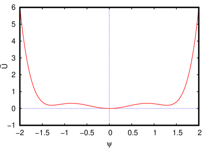
Figure 1: The scalar-field potential $\tilde{U}$ (48) as a function of $\psi$, assuming the values $\mu=1=\lambda$ and $\nu=9/32$ as in Ref.Brihaye .

For the RNBH, and the test-field approximation, which is the only problem that we analyze here, $\sigma(r)\equiv 1$, and

$$N(r)=-g_{tt}=1-\frac{2M}{r}+\frac{Q^{2}}{r^{2}}\,,$$ (49)

given by (1).

At this point it is important to remark that the theory considered so far is invariant with respect to a local phase transformation in the field $\Psi$. This local transformation is compensated by the gauge transformation in the electromagnetic potential. In particular, the theory is invariant with respect to a transformation

$$\omega = {\tilde{\omega}}+\zeta\,,$$ (50)

$$A_{t} = {\tilde{A}}_{t}-\zeta/q\,,$$ (51)

where $\zeta$ is a constant. This can be appreciated by a direct substitution in the full-fledged set of equations Herdeiro2020 . Nonetheless, this invariance is apparent from the field equations of the full theory since $A_{t}$ and $\omega$ appears always in a combination $\omega+qA_{t}$, which remains invariant under the above transformation, and also because the radial derivatives for $A_{t}$ are unaffected by this shift. As a consequence, one can use a gauge different from the one of previous sections where

$$\tilde{\omega} = 0\,,$$ (52)

$${\tilde{A}}_{t} = V(r)=\frac{Q}{r_{H}}-\frac{Q}{r}\,.$$ (53)

This gauge was employed in Brihaye , and previously in Herdeiro2020 . Notice that under this gauge, the electric potential $V(r)$ vanishes at the horizon, but asymptotically it takes a non-zero value. In our case, whether one uses this or the original gauge where $\omega\neq 0$, it is irrelevant since our treatment is gauge invariant. Therefore the integrand (38) remains the same. In particular the integrand (V) takes the same form, except that we have to replace the mass term for the corresponding term obtained from the potential (48), and also taking $m\equiv 0$, and $\nabla_{\theta}\phi=0$, since in this scenario we are assuming only a time and radial dependency in the field. Thus, the integral (V) becomes

$$\int_{\mathcal{V}}\Big{[}\left(\mu^{2}-2\lambda\psi^{2}+3\nu\psi^{4}-\frac{q^{2}Q^{2}}{r_{H}^{2}}+\frac{q^{2}Q^{2}\left(r_{H}-r_{-}\right)}{r_{H}^{2}(r-r_{-})}\right)\psi^{2}$$

$$+g^{rr}(\psi^{\prime})^{2}\Big{]}\sqrt{-g}d^{4}x=0\,,$$ (54)

where we used

$$\Psi^{*}\frac{\partial\tilde{U}\left(\Psi^{*}\Psi\right)}{\partial\Psi^{*}} = \Psi^{*}\left[\mu^{2}\Psi-2\lambda\left(\Psi^{*}\Psi\right)\Psi+3\nu\left(\Psi^{*}\Psi\right)^{2}\Psi\right]$$ (55)

$$= \mu^{2}\psi^{2}-2\lambda\psi^{4}+3\nu\psi^{6}\,.$$

Unlike the scenario with no self-interaction, the integrand in (VI) has not a definite sign due to the presence of the self-interaction terms, notably,

$$\Lambda(\psi)\equiv\psi^{2}\left(\mu^{2}_{\rm eff,\infty}-2\lambda\psi^{2}+3\nu\psi^{4}\right)\,,$$ (56)

where $\mu^{2}_{\rm eff,\infty}=\mu^{2}-\frac{q^{2}Q^{2}}{r_{H}^{2}}$ corresponds to the mass introduced in (17) for the non-self-interacting model, and like in that model, $\mu^{2}_{\rm eff,\infty}\geq 0$ so that the boson field also behaves asymptotically like in (16).

In this way the integral (VI) reads

$$\int_{\mathcal{V}}\Big{[}\Lambda(\psi)+\frac{q^{2}Q^{2}\left(r_{H}-r_{-}\right)}{r_{H}^{2}(r-r_{-})}\psi^{2}+g^{rr}(\psi^{\prime})^{2}\Big{]}\sqrt{-g}d^{4}x=0\,,$$ (57)

or even

$$\int_{\mathcal{V}}\Big{[}\mu^{2}_{\rm eff}(r)\psi^{2}+\Sigma(\psi)\psi^{2}+g^{rr}(\psi^{\prime})^{2}\Big{]}\sqrt{-g}d^{4}x=0\,,$$ (58)

where

$$\Sigma(\psi)\equiv\psi^{2}\left(-2\lambda+3\nu\psi^{2}\right)\,,$$ (59)

$$\mu^{2}_{\rm eff}(r)\equiv\mu^{2}_{\rm eff,\infty}+\frac{q^{2}Q^{2}\left(r_{H}-r_{-}\right)}{r_{H}^{2}(r-r_{-})}\,,$$ (60)

is a position-dependent effective squared mass.

The integrands in (57) or (58) are not positive semidefinite (i.e. they can be negative) due to the presence of $\Lambda(\psi)$ and $\Sigma(\psi)$, respectively. The terms containing the charges and the kinetic term (the one with the radial derivative) are positive semidefinite for $r\geq r_{H}$. In particular, $\Lambda$ is negative at the two minima corresponding to $\psi_{\rm\pm}^{\rm\Lambda}=\pm\sqrt{\frac{2\lambda}{9\nu}\left[1+\sqrt{1-\frac{9\nu\mu^{2}_{\rm eff,\infty}}{4\lambda^{2}}}\right]}$ and $\Sigma$ is also negative at the two minima $\psi_{\pm}^{\Sigma}=\pm\sqrt{\frac{\lambda}{3\nu}}$. Thus, the integrand in (VI) has no definite sign. Figures 2 and 3 depict $\Lambda$, and $\Sigma$, respectively, for values of the parameters used in Brihaye , showing that both quantities can be negative, namely, at the two minima. As a consequence, a no-hair theorem cannot be established in this case. Not only that theorem cannot be established for this kind of self-interacting scalar field potential, but, as we stressed before, several authors have showed that the presence of this kind of potential allows for the existence of non-trivial charged clouds, termed Q-clouds Hong2020 ; Herdeiro2020 ; Brihaye . As argued in Herdeiro2020 ; Brihaye these clouds can exist even in a Schwarzschild background, but in the presence of a test electric field.

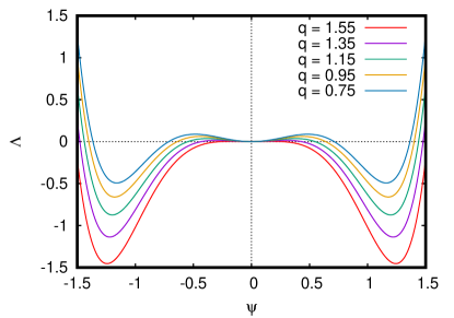
Figure 2: The function $\Lambda(\psi)$ (56) for different values of $q$, taking $\mu=1=\lambda$ and $\nu=9/32$ as in Fig.1. Here we assume $Q=0.09$ and $r_{H}=0.15$. The minima are located at $\psi_{\rm\pm}^{\rm\Lambda}$ where $\Lambda(\psi)$ is negative.

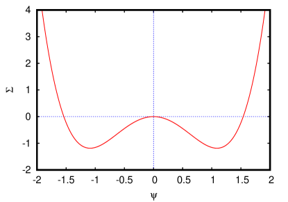
Figure 3: The function $\Sigma(\psi)$ (59) taking $\mu=1=\lambda$ and $\nu=9/32$ as in Fig.1. The minima are located at $\psi^{\Sigma}_{\pm}\approx\pm 1.0887$ where $\Sigma(\psi)$ is negative.

For the extremal RNBH $(r_{H}^{\rm ext}=M=|Q|)$ the integral (58) keeps the same form, except that $\mu^{2}_{\rm eff}(r)=\mu^{2}_{\rm eff,\infty,ext}=\mu^{2}-q^{2}$ is a non-negative constant, and

$$N(r)=\frac{(r-M)^{2}}{r^{2}}=g^{rr},\qquad\sigma^{2}(r)=1.$$ (61)

More specifically the integrand in (58) reduces to

$$I=\left(\mu^{2}-q^{2}-2\lambda\psi^{2}+3\nu\psi^{4}\right)\psi^{2}+\frac{\left(r-M\right)^{2}}{r^{2}}\left(\partial_{r}\psi\right)^{2}\;,$$ (62)

which does not have a definite sign. Therefore, one cannot establish a no-hair theorem either in the extremal scenario. Figure 4 depicts the term

$$\Lambda_{\rm ext}(\psi)\equiv\left(\mu^{2}-q^{2}-2\lambda\psi^{2}+3\nu\psi^{4}\right)\psi^{2}\,,$$ (63)

that appears in the integrand (62). We can rewrite this function as

$$\Lambda_{\rm ext}(\psi)=\left[3\nu\left(\psi^{2}-\frac{\lambda}{3\nu}\right)^{2}+\left(\mu^{2}_{\rm eff,\infty,\rm ext}-\frac{\lambda^{2}}{3\nu}\right)\right]\psi^{2}.$$ (64)

which indicates that when $\mu^{2}_{\rm eff,\infty,\rm ext}\geqslant\lambda^{2}/3\nu$ the integrand of the integral (58) is positive semidefinite, in which case, the only possible Q-cloud solution are the trivial ones $\psi(r)\equiv 0$ and $\psi(r)=\pm\sqrt{\frac{\lambda}{3\nu}}$ when $\mu^{2}_{\rm eff,\infty,\rm ext}=\lambda^{2}/3\nu$ or $\psi(r)\equiv 0$ when $\mu^{2}_{\rm eff,\infty,\rm ext}>\lambda^{2}/3\nu$. These are trivial solutions of Eq.(VI.1) (see below) when $M=Q$ which correspond to the three minima ($\psi=\pm\sqrt{\frac{\lambda}{3\nu}}$, $\psi=0$) of the potential which is introduced below in Eq.(68), and when assuming the extremal case (denoted $U_{\rm eff}^{\rm ext}$ in the main text). This minima correspond also to the zeros of $\Lambda_{\rm ext}(\psi)$. Notice that the two minima $\psi_{\pm}^{\Lambda}$ associated with $\Lambda(\psi)$ degenerate in the extremal case when $\mu^{2}_{\rm eff,\infty,\rm ext}=\lambda^{2}/3\nu$ and become two zeros of $\Lambda_{\rm ext}(\psi)$ (cf. the discussion at the end of Sec. VI.1). Notwithstanding, as we show below, there exist non-trivial solutions in the near extremal scenario when $\mu^{2}_{\rm eff,\infty,\rm ext}<\lambda^{2}/3\nu$.

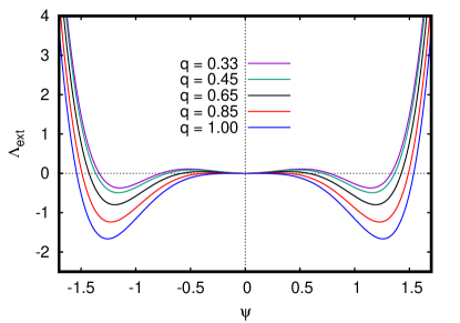
Figure 4: The function $\Lambda_{\rm ext}(\psi)$, taking $\mu=1=\lambda$ and $\nu=9/32$ for different values of $q$ in the extremal Reissner-Nordstrom scenario.

VI.1 Subextremal Q-clouds solutions

In order to find Q-cloud solutions we solve numerically the radial equation associated with the scalar field $\psi(r)$:

$$N^{2}(r)\psi^{\prime\prime}+\left[\frac{2}{r}N(r)+N^{\prime}(r)\right]N(r)\psi^{\prime}+\left(\tilde{\omega}+q\tilde{A}_{t}\right)^{2}\psi$$

$$=\frac{1}{2}\frac{\partial\tilde{U}}{\partial\psi}N(r)=\left(\mu^{2}\psi-2\lambda\psi^{3}+3\nu\psi^{5}\right)N(r)\,,$$ (65)

in the background of a subextremal RNBH, where $N(r)$ is given by (49), $\tilde{\omega}$ and $\tilde{A}_{t}$ by (52) and (53), respectively. Equation (VI.1) is solved by implementing the following regularity conditions for first and second derivatives at the horizon $r_{H}$:

$$\psi^{\prime}_{H} = \frac{1}{2N^{\prime}(r)}\frac{\partial{\tilde{U}}}{\partial\psi}\Big{|}_{r=r_{H}}$$ (66)

$$= \frac{r_{H}^{3}\left(\mu^{2}\psi_{H}-2\lambda\psi^{3}_{H}+3\nu\psi^{5}_{H}\right)}{\left(r_{H}^{2}-Q^{2}\right)}\,,$$

$$\psi^{\prime\prime}_{H} = \frac{\psi^{\prime}_{H}}{4N^{\prime}(r_{H})}\left[\frac{\partial^{2}\tilde{U}}{\partial\psi^{2}}\Big{|}_{r=r_{H}}-\frac{4}{r_{H}}N^{\prime}(r_{H})-3N^{\prime\prime}(r_{H})\right]$$ (67)

$$- \frac{q^{2}Q^{2}\psi_{H}}{2\left[r^{2}_{H}N^{\prime}(r_{H})\right]^{2}}+\frac{N^{\prime\prime}(r_{H})}{2\left[2N^{\prime}(r_{H})\right]^{2}}\frac{\partial{\tilde{U}}}{\partial\psi}\Big{|}_{r=r_{H}}$$

$$= \frac{\psi_{H}^{\prime}}{4\left[r_{H}^{2}-Q^{2}\right]}\Big{[}2\left(\mu^{2}-6\lambda\psi^{2}_{H}+15\nu\psi^{4}_{H}\right)r_{H}^{3}$$

$$+ 2r_{H}-\frac{8Q^{2}}{r_{H}}\Big{]}-\frac{q^{2}Q^{2}r_{H}^{2}\psi_{H}}{2\left[r_{H}^{2}-Q^{2}\right]^{2}}$$

$$- \frac{\left(\mu^{2}\psi_{H}-2\lambda\psi^{3}_{H}+3\nu\psi^{5}_{H}\right)\left(r_{H}^{2}-2Q^{2}\right)r_{H}^{2}}{2\left[r_{H}^{2}-Q^{2}\right]^{2}}\;,$$

where $\psi_{H}\equiv\psi(r_{H})$, $\psi^{\prime}_{H}\equiv\psi^{\prime}(r_{H})$ and $\psi^{\prime\prime}_{H}\equiv\psi^{\prime\prime}(r_{H})$.

Equation (VI.1) is solved numerically given the parameters $\lambda$, $\nu$, $\mu$ and $q$, and fixing the value of the horizon $r_{H}$ and the charge $Q$ of the RNBH. The values for $\psi^{\prime}_{H}$ and $\psi^{\prime\prime}_{H}$ are determined once the specific value for $\psi_{H}$ is provided. This value is found by a shooting method such that the field $\psi(r)$ vanishes asymptotically. At this point, it is important to stress that the field $\psi(r)$ is indeed submitted to an effective potential that in the asymptotic region takes the form [cf. Eq.(VI.1)]

$$U_{\rm eff}=\mu_{\rm eff,\infty}^{2}\psi^{2}-\lambda\psi^{4}+\nu\psi^{6},$$ (68)

where $\mu_{\rm eff,\infty}^{2}=\mu^{2}-q^{2}Q^{2}/r_{H}^{2}$.

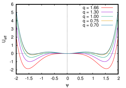
Figure 5: The effective potential $U_{\rm eff}$ (68) taking $\mu=1=\lambda$, $\nu=9/32$, $Q=0.09$, and $r_{H}=0.15$, for different values of $q$.

Figure 5 depicts the effective potential (68) associated with different values for $q$ taking $\mu=\lambda=1$, $\nu=9/32$, $r_{H}=0.15$ and $Q=0.09$. The shooting method aims at the local minimum of this effective potential located at $\psi=0$, where $U_{\rm eff}$ vanishes, starting from trial values $\psi_{H}$ that depend on the value for $q$. In general a numerical exploration shows that this trial values (assuming only positive ones for concreteness) are such that $0<\psi_{H}<\psi_{\rm min}^{+}$ where $\psi_{\rm min}^{+}$ is associated with one of the two global minima of $U_{\rm eff}$ given by $\psi_{\rm min}^{+}$, with $\psi_{\rm min}^{\pm}=\pm\sqrt{\frac{\lambda}{3\nu}\left[1+\sqrt{1-\frac{3\mu_{\rm eff,\infty}^{2}\nu}{\lambda^{2}}}\right]}$. As we stressed above, the local minimum of $U_{\rm eff}$ is at $\psi=0$ and corresponds to the asymptotic value of the field $\psi(r)$. Therefore for some $q$ the field $\psi(r)$ must climb one of the local maximum of $U_{\rm eff}$ before reaching the local minimum. A bad shooting can make the field to oscillate around any of the two $\psi_{\rm max}$ associated with the local maxima of $U_{\rm eff}$ [cf. Fig. 8 below] or can make the field to go to $\pm\infty$. As remarked in Brihaye , giving $Q$, $\mu$ and $r_{H}$, the charge $q$ is limited from above by the condition $\mu_{\rm eff,\infty}^{2}\geq 0$, which corresponds to $|q|\leq\mu r_{H}/|Q|$. On the other hand, the zeros of $U_{\rm eff}$ are given by $\psi=0$ and $\psi=\pm\sqrt{\frac{\lambda}{2\nu}\left[1\pm\sqrt{1-\frac{4\mu_{\rm eff,\infty}^{2}\nu}{\lambda^{2}}}\right]}$. So when $\mu_{\rm eff,\infty}^{2}=\frac{\lambda^{2}}{4\nu}$, we see that the charge $q$ is limited from below $|q|_{\rm min}\lesssim q$ where $|q|_{\rm min}\approx\frac{r_{H}\mu}{|Q|}\sqrt{1-\frac{\lambda^{2}}{4\nu\mu^{2}}}$, assuming $\nu>0$. All this analysis is qualitative, but gives a fair description of the actual numerical study. In particular, the lower bound $|q|_{\rm min}$ is approximate, since in this analysis we are neglecting the contribution of the metric function $N(r)$ in $U_{\rm eff}$ and taking it as if $N(r)=1$. Moreover, for this particular value of $\mu_{\rm eff,\infty}^{2}$ the potential $U_{\rm eff}$ “degenerate” in that the two global minima $\psi_{\rm min}^{\pm}$ become also two of its three zeros at $\psi=\pm\sqrt{\frac{\lambda}{2\nu}}$. In this degenerate situation $\psi(r)=\psi_{\rm min}^{+}$ is an approximate solution. So when $|q|\rightarrow|q|_{\rm min}$ the actual positive value $\psi_{H}\rightarrow\psi_{\rm min}^{+}$, and since in this limit situation $\psi_{\rm min}^{+}$ is an approximate solution for the field, then the field $\psi(r)$ remains very close to the constant value $\psi_{\rm min}^{+}$ for a relatively large values $r$ and then interpolates to the asymptotic value $\psi=0$ associated with $\psi(r\rightarrow\infty)$, and the actual numerical solution resembles a step function, as we can appreciate from Fig.  6. This figure depicts some examples of Q-clouds solutions $\psi(r)$ for different values of $q$ for a RNBH with charge $Q=0.09$, horizon $r_{H}=0.15$, and a scalar field with mass $\mu=1$. As $q$ approaches its minimum value, we see that the Q-cloud solution start looking like a step function. Our results are in agreement with those obtained in Brihaye .

Figure 7 shows the quantity $\Lambda(\psi)$ that appears in Eq. (57), when using the solutions $\psi(r)$ that are plotted in Fig. 6. From Fig. 7 we appreciate that $\Lambda(\psi)$ has indeed negative contributions to the integrand of the integral (57). The fact that the integrand has negative and positive contributions allow us to understand why this integral vanishes when $\psi(r)$ is not necessarily the trivial solution $\psi(r)\equiv 0$, in contrast with the scenario of Sec. V where the self-interaction terms are absent leading to an integrand which is never negative and therefore implying that $\psi(r)\equiv 0$ is the only possible well behaved solution.

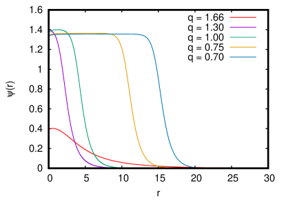
Figure 6: Q-cloud solutions $\psi(r)$ for a RNBH with $Q=0.09$, $r_{H}=0.15$, and $\mu=1=\lambda$, $\nu=9/32$ taking different values for $q$.

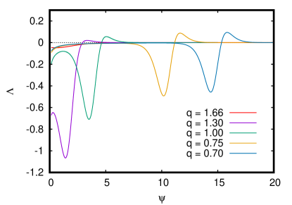
Figure 7: The quantity $\Lambda(\psi)$ associated with the solutions of Fig. 6. Notice that this quantity can be negative and contributes non-trivially to the integral (57).

Figure 8 shows three numerical solutions for $\psi(r)$ with $q=1$ associated with three different (albeit very similar) values $\psi_{H}$. The two oscillating solutions correspond to the two values $\psi_{H}$ that undershoot and overshoot the desired asymptotic value $\psi=0$, and which asymptotically oscillate around $\psi_{\rm max}$ associated with the local maxima of $U_{\rm eff}$, given by $\psi_{\rm max}\approx\pm 0.6175$ . These two values are represented by the horizontal dotted lines. The non-oscillating solution corresponds to the optimal shooting value $\psi_{H}$ leading to an asymptotically vanishing solution.

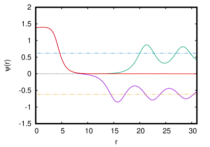
Figure 8: Solutions $\psi(r)$ (solid lines) with $q=1$ for three different values of $\psi_{H}$ within a RNBH with $Q=0.09$, $r_{H}=0.15$, $\mu=1=\lambda$ and $\nu=9/32$. The three solutions correspond to $\psi_{H}$: 1.3820 (purple line), 1.381958 (green line) and 1.381959590 (red line). The horizontal dotted lines represent the two values $\psi_{\rm max}\approx\pm 0.6175$ associated with the local maxima of the effective potential $U_{\rm eff}$ depicted in Fig.5 for $q=1$. The solution corresponding to an asymptotically vanishing field, which is the relevant for the current analysis, is marked in red color.

We have also obtained Q-cloud solutions in the near extremal RNBH scenario $Q\approx M$ which are consistent with those reported in Hong2020 . In this scenario the charge $q$ is bounded as follows $q_{\rm min}\lesssim q\lesssim\mu$, where $q_{\rm min}\approx 1/3$, and this value is obtained from $|q_{\rm min}|$ in the near extremal limit and when $\nu$ saturates the bound $\lambda^{2}/4\mu$ required for the scalar-field potential (48) to have a true vacuum at $\Psi=0$. Figure 9 shows four solutions of this kind as $Q$ approaches $M$ and Fig. 10 shows the effective potential associated with these solutions. From the regularity conditions (66) and (67) we appreciate that as $Q\rightarrow M$ the derivatives diverge at the horizon, a feature that can be appreciated also in Fig. 9. Due to this divergent behavior at the horizon, the exact extremal case $(Q=M)$ requires a separate analysis that demands a different numerical technique Garciaetal . Moreover, this analysis is also necessary to prove that if a non-trivial physically meaningful solution exists for the field $\psi(r)$ in the exact extremal scenario, then the kinetic term in the integral (57), namely $g^{rr}(\psi^{\prime})^{2}$, remains well behaved, notably at the horizon, despite a divergent $\psi^{\prime}_{H}$. At this respect it is also interesting to remark that non-trivial Q-cloud solutions in the extremal scenario with bounded derivatives at the horizon are absent Garciaetal , and the only ones allowed that have bounded derivatives are the trivial ones corresponding to the zeros of $\Lambda_{\rm ext}(\psi)$ (cf. Fig. 4) or equivalently, to the extrema (minima and maxima) of $U_{\rm eff}^{\rm ext}$ depicted by Fig. 11. Thus, in the near extremal case when $q$ approaches $1/3$ something similar happens to the subextremal solutions when $q\approx q_{\rm min}$. Namely, the solutions have a “step function” shape, where $\psi(r)$ remains near the global minima of $U_{\rm eff}$ for larger values of $r$ as $q\rightarrow 1/3$, and then interpolates to the local minimum of $U_{\rm eff}$ associated with the asymptotic value $\psi\rightarrow 0$ passing through a local maximum. This behavior is depicted by Fig. 12.

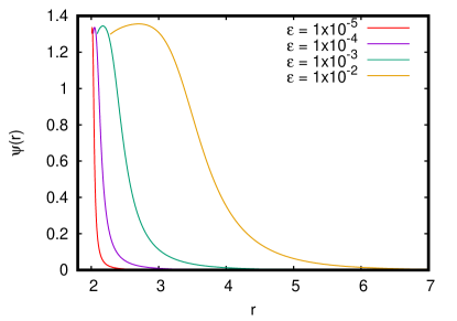
Figure 9: Q-cloud solutions $\psi(r)$ for near extremal RNBH $Q\approx M$, taking $M=2$, $\mu=1=\lambda$, $\nu=9/32$ and $q=0.8$. The charge of the black hole is taken to be $Q=(1-\varepsilon)M$ with $\varepsilon=10^{-2}$, $10^{-3}$, $10^{-4}$ and $10^{-5}$.

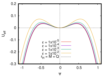
Figure 10: The effective potential $U_{\rm eff}$ (68) associated with the radial solutions for the near extremal RNBH (Fig. 9) taking $\lambda=1$, $\nu=9/32$, $\mu=1$ and $q=0.8$. The charge of the black hole is taken to be $Q=(1-\varepsilon)M$ with $\varepsilon=10^{-2}$, $10^{-3}$, $10^{-4}$ and $10^{-5}$. For reference, the exact extremal case $r_{H}=M=Q$ is depicted by the black dashed line.

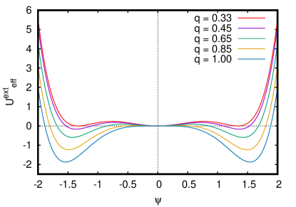
Figure 11: The effective potential $U^{\rm ext}_{\rm eff}$ (68) taking $\mu=1=\lambda$, $\nu=9/32$, and $Q=r_{H}=0.15$, for different values of $q$.

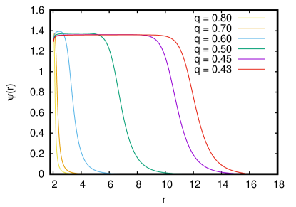
Figure 12: Q-cloud solutions $\psi(r)$ for near extremal RNBH $Q\approx M$, taking $M=2$, $\mu=1=\lambda$, $\nu=9/32$. The charge of the black hole is taken to be $Q=(1-\varepsilon)M$ with $\varepsilon=10^{-4}$ and for values $q$ approaching $1/3$.

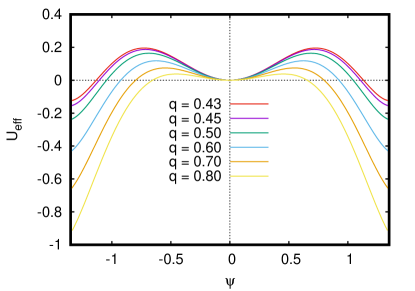
Figure 13: The effective potential $U_{\rm eff}$ (68) associated with the radial solutions for the near extremal RNBH (Fig. 12) taking $\lambda=1$, $\nu=9/32$ and $\mu^{2}=1$ and for different values of $q$ that approach the positive value $q_{\rm min}^{\rm ext}\approx 1/3$ with $Q=(1-\varepsilon)M$ and $\varepsilon=10^{-4}$.

As mentioned before, in the exact extremal scenario $\mu^{2}_{\rm eff}(r)$ given by (60) reduces to $\mu^{2}_{\rm eff}(r)=\mu^{2}_{\rm eff,\infty,ext}=\mu^{2}-q^{2}$ which is not position dependent anymore, and then the extrema (minima and maxima) of $U_{\rm eff}^{\rm ext}$ become exact but trivial Q-cloud solutions. Moreover, when $\mu^{2}_{\rm eff,ext,\infty}=\frac{\lambda^{2}}{3\nu}$, the effective potential (68) with $\mu^{2}_{\rm eff}=\mu^{2}_{\rm eff,ext,\infty}$, has only one global minima at $\psi=0$ (see Fig. 14), which is the only possible solution since in this case the function $\Lambda_{\rm ext}(\psi)$ is positive semidefinite and therefore the integral (57) only holds if $\psi(r)\equiv 0$. In this particular extremal scenario there is not even a real valued $q$ that satisfies the condition $\mu^{2}_{\rm eff,ext,\infty}=\mu^{2}-q^{2}=\frac{\lambda^{2}}{3\nu}$ unless $\nu\geq\lambda^{2}/3\mu^{2}$.

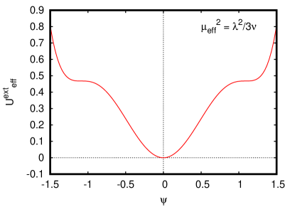
Figure 14: The effective potential $U^{\rm ext}_{\rm eff}$ (68) for an extremal RNBH ($r_{H}=|Q|=M$) taking $\mu=1=\lambda$, $\nu=9/32$, and for $\mu_{\rm eff,ext,\infty}^{2}=\lambda^{2}/3\nu=32/27$.

VII Conclusion

A massive, charged and complex-valued scalar field coupled to a Reissner-Nordstrom black hole has been studied for the subextremal and extremal scenarios, by imposing regularity conditions on the field, notably, in the radial part. When the scalar-field potential has no self-interactions terms it is not possible to find non-trivial superregular numerical solutions or scalar clouds (i.e. solutions where the field and its radial derivatives are bounded in the domain of outer communication of the BH and at the BH horizon as well). The extremal scenario with an extremal scalar field $(|q|=\mu)$, dubbed double extremal, was previously studied by Degollado $\&$ Herdeiro DegolladoHerdeiro2013 reporting non-trivial solutions, but it is unclear to what extent those solutions are regular at the horizon, given that using an integral method we have proven a theorem establishing that such non-trivial configurations cannot exist even if one allows a certain singular behavior on the radial derivative of the field at the extremal horizon while keeping the kinetic scalars associated with the boson field bounded there. Therefore, this conclusion casts doubts about the physical significance of the solutions found in DegolladoHerdeiro2013 . On the other hand, by implementing the same integral method to the case where the scalar-field potential has self-interaction terms, it is not possible to prove a similar theorem, which in turn provides a heuristic justification and understanding for the existence of regular and spherically symmetric cloud solutions within this variant of the theory (termed Q-clouds) which have been reported recently by several authors Hong2020 ; Herdeiro2020 ; Brihaye and that we have reproduced here in the background of a subextremal (including a near extremal) RNBH. Finally, given that the radial derivative of the field may diverge at the BH horizon in the extremal scenarios (cf. Hod2012 ; Hod2015 for non-charged and charged clouds in the backgrounds of an extremal Kerr and an extremal Kerr-Newman black holes, respectively) while keeping the solutions for the clouds physically meaningful Garciaetal , a more detailed study is in order for the numerical analysis of Q-clouds in the presence of an exact extremal RN black hole and not only in the near extremal limit Garciaetal .

Appendix A Non-existence of bound states for a free scalar field around Reissner-Nordstrom BH

It is instructive to recover the no-hair theorem presented in Sec. V in a much more simplified fashion. We begin by considering Eq.(13) for the radial function $R=R(r)$:

$$\left(\Delta R^{\prime}\right)^{\prime}=\left[\left(K_{l}+\mu^{2}r^{2}\right)-\frac{\mathcal{H}^{2}}{\Delta}\right]R,$$ (69)

multiplying both sides by $R$ and integrating both sides from $r_{H}$ to infinity, we obtain

$$\int_{r_{H}}^{\infty}R\left(\Delta R^{\prime}\right)^{\prime}dr=\int_{r_{H}}^{\infty}\left[K_{l}+\mu^{2}r^{2}-\frac{\mathcal{H}^{2}}{\Delta}\right]R^{2}dr\,.$$ (70)

Integrating by parts the left-hand side of previous equation reads

$$\int_{r_{H}}^{\infty}R\left(\Delta R^{\prime}\right)^{\prime}dr=\left.R\Delta R^{\prime}\right|_{r_{H}}^{\infty}-\int_{r_{H}}^{\infty}\left(\Delta R^{\prime}\right)R^{\prime}dr\,.$$ (71)

Assuming the following conditions at the horizon and asymptotically [cf. Eq. (16)]

$$R(r_{H}),R^{\prime}(r_{H})<\infty\quad\text{(finite values at $r_{H}$)},$$ (72)

$$R(r\rightarrow\infty),R^{\prime}(r\rightarrow\infty)\rightarrow 0\,,$$ (73)

and given that $\Delta$ vanishes at the horizon,

$$\Delta_{H}\equiv r_{H}^{2}-2Mr_{H}+Q^{2}=0,$$

we conclude

$$\left.R\Delta R^{\prime}\right|_{r_{H}}^{\infty}=0.$$ (74)

Therefore Eq. (70) reduces to

$$\int_{r_{H}}^{\infty}\Big{[}\Delta R^{\prime 2}+\alpha(r)R^{2}\Big{]}dr=0,$$ (75)

where we have defined

$$\alpha(r)\equiv K_{l}+\mu^{2}r^{2}-\frac{\mathcal{H}^{2}}{\Delta}.$$ (76)

We observe that the first term $\Delta R^{\prime 2}$ is positive semi-definite, however, the second term $\alpha(r)R^{2}$ does not have an apparent definite sign. Nevertheless, below we prove that $\alpha(r)$ is not negative. Since $\mathcal{H}$ is given by Eq.(15) and

$$\Delta=\left(r-r_{H}\right)\left(r-r_{-}\right)\,,$$ (77)

then

$$\alpha(r)=K_{l}+\mu^{2}r^{2}-\frac{q^{2}Q^{2}}{r_{H}^{2}}\frac{\left(r-r_{H}\right)r^{2}}{\left(r-r_{-}\right)}.$$ (78)

Using

$$\frac{r-r_{H}}{r-r_{-}}=1+\frac{r_{-}-r_{H}}{r-r_{-}},$$ (79)

it is possible to rewrite equation (76) as

$$\alpha(r)=K_{l}+\left(\mu^{2}-\omega^{2}\right)r^{2}+\omega^{2}r^{2}\frac{\left(r_{H}-r_{-}\right)}{\left(r-r_{-}\right)}\,.$$ (80)

We now appreciate that the function $\alpha(r)$ is positive semidefinite for $r\geqslant r_{H}$ and $\mu^{2}\geq\omega^{2}$, and $r_{H}\geq r_{-}$, which includes the extremal scenario. In the subextremal case $r_{H}>r_{-}$, the function $\alpha(r)$ is strictly positive. Therefore the integrand that appears in the integral (75) is non-negative, and for this integral to vanish it is necessary that each term in the integrand vanishes identically for all $r\geq r_{H}$. In particular, if $\mu^{2}>\omega^{2}$,

$$R^{\prime}(r)\equiv 0\quad\text{and}\quad R(r)\equiv 0,$$ (81)

which leads to the trivial solution $\Psi\equiv 0$. We conclude that there are no bound states when the scalar field is coupled to a subextremal Reissner-Nordstrom BH with $\mu^{2}>\omega^{2}$. In the extremal case $(r_{H}=M=Q)$ the function $\alpha(r)$ reduces to

$$\alpha(r)=K_{l}+\left(\mu^{2}-\omega^{2}\right)r^{2},$$ (82)

where $\omega^{2}=q^{2}$ in this case. Again, if $\mu^{2}>\omega^{2}$, then $\alpha(r)$ is strictly positive for all $r\geq r_{H}$, and the same conclusion follows about the absence of non-trivial scalar clouds.

Finally, when focused on the scenario studied by Degollado and Herdeiro DegolladoHerdeiro2013 about charged scalar clouds in the extremal RNBH with an extremal test field with $\mu=|q|$ then

$$\alpha(r)=K_{l}=l(l+1)\geqslant 0\,.$$ (83)

Thus $\alpha(r)$ is nonzero except for $l=0$ (i.e. spherically symmetric clouds), and then the integral (75) vanishes for all $l\geq 0$ only if the radial function satisfies for all $r\geq r_{H}=M$:

$$R^{\prime}(r)\equiv 0\quad\text{and}\quad R(r)\equiv 0,\quad\text{for}\quad l\neq 0,$$ (84)

and

$$R^{\prime}(r)\equiv 0\quad\text{and}\quad R(r)\equiv{\rm const.},\quad\text{for}\quad l=0\,.$$ (85)

Since we demand that $R(r\rightarrow\infty)\rightarrow 0$, then $R(r)\equiv 0$ also for $l=0$. Thus, even in the particular extremal scenario of Ref. DegolladoHerdeiro2013 , our analysis shows that non-trivial clouds are not possible.

The final conclusion is that non-trivial regular bound states for a free scalar field (massive and charged) in the background of a Reissner-Nordstrom black hole, extremal or subextremal, are absent.

References

• (1) G. García and M. Salgado, Phys. Rev. D 99, 044036 (2019).
• (2) C. Herdeiro, and E. Radu, Phys. Rev. Lett. 112, 221101 (2014).
• (3) C. Herdeiro, and E. Radu,Class. Quant. Grav. 32, 144001 (2015).
• (4) G. García and M. Salgado, Phys. Rev. D 101, 044040 (2020).
• (5) S. Hod, Phys. Rev. D 86, 104026 (2012); Phys. Rev. D 86, 129902(E) (2012).
• (6) S. Hod, Phys. Lett. B 751, 177-183 (2015).
• (7) C. Benone, L. C. B. Crispino, C. Herdeiro, and E. Radu, Phys. Rev. D 90, 104024 (2014).
• (8) J. C. Degollado and C. A. R. Herdeiro, Gen. Relativ. Gravit. 45, 2483-2492 (2013).
• (9) S. A. Teukolsky, Phys. Rev. Lett. 29, 1114 (1972).
• (10) G. García, P. Grandclément, E. Gourgoulhon, and M. Salgado, (in preparation)
• (11) P. Grandclément, C. Somé and E. Gourgoulhon, Phys. Rev. D 90, 024068 (2014).
• (12) J. Bekenstein, Phys. Rev. D 5, 1239 (1972).
• (13) M. Heuler, Helv. Phys. Acta 69, 501 (1996).
• (14) E. Ayón-Beato, Class. Quant. Grav. 19, 5465 (2002).
• (15) J. P. Hong, M. Suzuki, and M. Yamada, Phys. Lett. B 803, 135324 (2020).
• (16) C. A. R. Herdeiro, and E. Radu, Eur. Phys. J. C 80, 390 (2020).
• (17) Y. Brihaye and B. Hartmann, arXiv:2009.08293v1 [qr-qc].
• (18) A. E. Mayo, and J. Bekenstein, Phys. Rev. D 54, 5059 (1996).
• (19) J. P. Hong, M. Suzuki, and M. Yamada, Phys. Lett. B 125, 111104 (2020).