Disorder in order: Localization without randomness in a cold atom system

Abstract

We present a mapping between the Edwards model of disorder describing the motion of a single particle subject to randomly-positioned static scatterers and the Bose polaron problem of a light quantum impurity interacting with a Bose-Einstein condensate (BEC) of heavy atoms. The mapping offers an experimental setting to investigate the physics of Anderson localization where, by exploiting the quantum nature of the BEC, the time evolution of the quantum impurity emulates the disorder-averaged dynamics of the Edwards model. Valid in any space dimension, the mapping can be extended to include interacting particles, arbitrary disorder or confinement, and can be generalized to study many-body localization. Moreover, the corresponding exactly-solvable disorder model offers means to benchmark variational approaches used to study polaron physics. Here, we illustrate the mapping by focusing on the case of an impurity interacting with a one-dimensional BEC through a contact interaction. While a simple wave function based on the expansion in the number of bath excitations misses the localization physics entirely, a coherent state Ansatz combined with a canonical transformation captures the physics of disorder and Anderson localization.

I Introduction

Coupling a particle to the collective excitations of a system with many degrees of freedom can radically alter the particle’s properties. While this paradigm has been first proposed by Landau and Pekar to describe how the interaction between electrons and lattice phonons gives rise to quasiparticles named polarons [1], it has been extended to give insight into numerous systems [2, 3], including ³He–⁴He mixtures [4], semiconductors [5] and high-temperature superconductors [6]. Although described by simple models such as the Fröhlich Hamiltonian and in spite of intensive efforts [7, 8, 9, 10, 11, 12, 13, 14, 15, 16, 17, 18, 19, 20, 21, 22], a comprehensive solution of the polaron problem still escapes theory. The advent of ultracold atoms allows the realization of polaron models with high tunability and brought means to probe such models, as evidenced by the recent observation of the Bose polaron spectral function in impurity-boson mixtures [23, 24, 25, 26, 27].

In this article, we bring together the seemingly disconnected fields of polarons and disorder. Following Anderson’s realization that quantum interference can hinder the diffusion of a particle to the point that it becomes localized [28], the interplay of disorder and quantum physics has been extensively studied, revealing intricate phenomena such as magnetoresistance [29, 30], coherent backscattering [31, 32, 33] and many-body localization [34, 35, 36, 37]. While Anderson localization was first observed in wave systems [38, 39], the development of cold atom physics allowed to achieve the localization of matter waves [40, 41] and realize the quantum kicked rotor model [42, 43] which can be mapped onto the Anderson model of disorder [44].

Here, we explore an alternative way to study the physics of disorder by establishing a mapping between the disorder-averaged motion of a single particle evolving through a random disorder potential, and that of an impurity immersed in a disorder-free Bose-Einstein condensate (BEC). This mapping, illustrated in Fig. 1, can experimentally be realized using a mass-imbalanced mixture of light impurities immersed in a bath of heavy bosons and provides a theoretical tool to include disorder effects in many-body approaches.

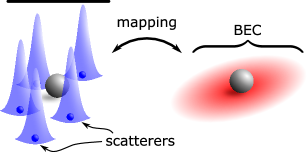
Figure 1: The disorder-averaged evolution —represented by the overline— of a particle subject to a random scattering potential (left) is mapped onto the time evolution of an impurity immersed in a homogeneous, disorder-free BEC (right).

Indeed, both the theoretical description of disorder and Bose polarons face challenges of different origins. While the rich physics of the Bose polaron problem arises from hard to capture many-body effects, performing the disorder average for even single-particle models is challenging. As such, a solution of the polaron problem can give insight into the corresponding disorder model, and conversely the disorder model can serve as an exactly solvable benchmark for polaron theories. To demonstrate this connection we show how a variational method applied to the study of impurity models can reproduce the exact short-time solution of the corresponding disorder model and discuss implications of the mapping for studies of polaron and disorder physics.

II The mapping

Many aspects of disorder physics such as Anderson localization are universal. They may depend on dimension and symmetries but not on specific details of the Hamiltonian, leaving freedom as to which model of disorder one studies. We consider the Edwards model [45, 46] that describes the evolution of a single particle through a medium of $N$ randomly-positioned static scatterers given by the Hamiltonian

$$\hat{H}_{\mathrm{Ed}}^{{\{{\mathbf{r}}_{i}\}}} =\dfrac{\hat{\mathbf{p}}^{2}}{2m_{\mathrm{I}}}+V(\hat{\mathbf{r}}), V(\hat{\mathbf{r}}) =\sum_{i=1}^{N}v(\hat{\mathbf{r}}-{\mathbf{r}}_{i}).$$ (1)

Here $\hat{\mathbf{r}}$ and $\hat{\mathbf{p}}$ are the position and momentum operators of the particle and $v(\hat{\mathbf{r}}-{\mathbf{r}}_{i})$ is the potential created by a scatterer at site ${\mathbf{r}}_{i}$. In one dimension and with contact interactions, this model is known as the random Kronig–Penney model (RKPM) [47, 48]. The randomness comes from the positions ${\mathbf{r}}_{i}$ of the scatterers, distributed e.g. uniformly in a volume $\Omega$. Denoting $\langle\hat{o}(t)\rangle_{\{{\mathbf{r}}_{i}\}}$ the expectation value of an observable $\hat{o}$ at time $t$ for a given realization of disorder $\{{\mathbf{r}}_{i}\}$, its disorder average is

$$\overline{\langle\hat{o}(t)\rangle}=\int_{\{{\mathbf{r}}_{i}\}}\langle\hat{o}(t)\rangle_{\{{\mathbf{r}}_{i}\}},$$ (2)

where $\int_{\{{\mathbf{r}}_{i}\}}=\Omega^{-N}\int d^{d}{\mathbf{r}}_{1}\dotsm d^{d}{\mathbf{r}}_{N}$ is the normalized integral over all possible scatterer positions ${\mathbf{r}}_{i}$.

We now show that for any observable $\hat{o}$ the disorder average 2 can be computed by means of a disorder-free polaron model. In this model one considers a system where a mobile impurity of position $\hat{\mathbf{r}}$ and momentum $\hat{\mathbf{p}}$ is immersed in a bosonic bath, described by the Hamiltonian

$$\hat{H} =\dfrac{\hat{\mathbf{p}}^{2}}{2m_{\mathrm{I}}}+\sum_{\mathbf{k}}\omega_{\mathbf{k}}\hat{b}^{\dagger}_{\mathbf{k}}\hat{b}_{\mathbf{k}}+\int_{{\mathbf{r}}^{\prime}}v(\hat{\mathbf{r}}-{\mathbf{r}}^{\prime})\hat{b}^{\dagger}_{{\mathbf{r}}^{\prime}}\hat{b}_{{\mathbf{r}}^{\prime}}$$ (3)

where $\omega_{\mathbf{k}}={\mathbf{k}}^{2}/2m_{\mathrm{B}}$ describes the dispersion relation of bosons at momentum ${\mathbf{k}}$ annihilated (created) by the operator $\hat{b}^{(\dagger)}_{\mathbf{k}}$, and $m_{\mathrm{I}}$ and $m_{\mathrm{B}}$ are the masses of the impurity and the bosons, respectively. Both species interact with the density-density interaction $v({\mathbf{r}})$.

To establish the mapping, we quench the system by preparing the impurity in a given wavepacket $|\psi\rangle$ and the bosons in a Bose-Einstein condensate (BEC) of $N$ non-interacting particles,

$$|\mathrm{BEC}\rangle=\dfrac{(\hat{b}_{{\mathbf{k}}=0}^{\dagger})^{N}}{\sqrt{N!}}|0\rangle=\int_{\{{\mathbf{r}}_{i}\}}|\{{\mathbf{r}}_{i}\}\rangle$$ (4)

where

$$|\{{\mathbf{r}}_{i}\}\rangle=\dfrac{\hat{b}^{\dagger}_{{\mathbf{r}}_{1}}\dotsm\hat{b}^{\dagger}_{{\mathbf{r}}_{N}}}{\sqrt{N!}}|0\rangle$$ (5)

denotes the state where the $N$ bosons have well-defined positions ${\mathbf{r}}_{i}$. The combined state of the system reads

$$|\Psi\rangle=|\psi\rangle\otimes|\mathrm{BEC}\rangle=\int_{\{{\mathbf{r}}_{i}\}}|\psi\rangle\otimes|\{{\mathbf{r}}_{i}\}\rangle.$$ (6)

Polaron model	Disorder model
Impurity	Particle
Heavy boson	Static scatterer
Interspecies interaction	Scattering potential
$N$-boson state $|\{{\mathbf{r}}_{i}\}\rangle$	Disorder configuration $\{{\mathbf{r}}_{i}\}$
BEC state	Sampling of disorder
Quantum measurement $\langle\hat{O}(t)\rangle$	Disorder average $\overline{\langle\hat{o}(t)\rangle}$

Table 1: Correspondence between the heavy Bose polaron and Edwards model of disorder.

For infinitely massive bosons, $m_{\mathrm{B}}/m_{\mathrm{I}}=\infty$, the time evolution of each state $|\psi\rangle\otimes|\{{\mathbf{r}}_{i}\}\rangle$ contributing to the superposition  4 can be determined exactly. The boson kinetic energy drops out and the total Hamiltonian commutes with the bosonic position operators. Hence, the bosons remain in the state $|\{{\mathbf{r}}_{i}\}\rangle$. Physically, the heavy bosons’ positions are not affected by the interaction with the impurity. On the other hand, the impurity views the $N$ localized bosons as scatterers at positions ${\mathbf{r}}_{i}$ and evolves through the Edwards Hamiltonian 1 such that the system evolves into

$$|\Psi(t)\rangle=\int_{\{{\mathbf{r}}_{i}\}}\Big{[}e^{-i\hat{H}_{\mathrm{Ed}}^{{\{{\mathbf{r}}_{i}\}}}t}|\psi\rangle\Big{]}\otimes|\{{\mathbf{r}}_{i}\}\rangle;$$ (7)

i.e., the system evolves as a superposition over all possible disorder realizations.

Hence, the expectation value of any observable of the impurity $\hat{O}=\hat{o}\otimes 1$ with respect to the state $|\Psi(t)\rangle$,

$$\langle\hat{O}(t)\rangle=\int_{\{{\mathbf{r}}_{i}\}}\langle\psi|e^{i\hat{H}_{\mathrm{Ed}}^{{\{{\mathbf{r}}_{i}\}}}t}\hat{o}e^{-i\hat{H}_{\mathrm{Ed}}^{{\{{\mathbf{r}}_{i}\}}}t}|\psi\rangle=\overline{\langle\hat{o}(t)\rangle},$$ (8)

realizes the disorder average $\overline{\langle\hat{o}(t)\rangle}$ 2. All states in the superposition contribute equally to the measurement of $\hat{O}$, thus carrying out an average over all possible $\{{\mathbf{r}}_{i}\}$ configurations. In other words, the fact that the BEC is a quantum superposition with equal weight of orthogonal states $|\{{\mathbf{r}}_{i}\}\rangle$ enables disorder averaging in an analog way using quantum systems such as ultracold atoms. By contrast with a proposal in Ref. [49] where disorder is simulated using pinned atoms loaded in an optical lattice, in the present work randomness is simulated using the quantum superposition in which the bosons are prepared, similar to a suggestion made for spin systems in Ref. [50].

The correspondence between the two models is summarized in Table 1. We emphasize that $\langle\hat{O}(t)\rangle$ and $\overline{\langle\hat{o}(t)\rangle}$ have very different meanings. While $\langle\hat{O}(t)\rangle$ represents a many-body measurement of the impurity evolving through the interaction with a bath of heavy bosons, $\overline{\langle\hat{o}(t)\rangle}$ corresponds to the measurement of the corresponding observable in the single-particle Edwards model averaged over many classical realizations of disorder.

III Generalizations

Most assumptions made for simplicity in the proof can be relaxed, as long as the crucial ingredient that the $|\{{\mathbf{r}}_{i}\}\rangle$ are eigenstates of the Hamiltonian remains valid. In particular, the proof applies to any dimension. Moreover, it is possible to include arbitrary confining potentials or interactions between the bosons, and even prepare the boson bath in a mixed state. In all these cases, the corresponding distribution of disorder would not be uniform but set by the boson state.

Crucially, the mapping holds also for multiple particles. That way, it is possible to simulate transport properties of realistic metals or to consider interactions between the impurities in order to investigate the interplay of many-body and disorder effects. The latter scenario has recently been considered in a study of many-body localization, where the thermalization properties of mass-imbalanced mixtures was investigated [51].

The mapping holds when the bosons have a mass exceedingly large compared to the impurity. When this is not the case, the feedback of the interaction with the impurity as well as eventual interactions among bosons will induce dynamics of the bath, defining a characteristic timescale $\tau_{\phi}$ diverging with $m_{\mathrm{B}}/m_{\mathrm{I}}$. In the disorder model, this would correspond to dynamical disorder and cause dephasing. While this may hinder the observation of phenomena associated with disorder, one could conversely take advantage of the presence of $\tau_{\phi}$ to investigate the physics of dephasing in a controlled manner. Furthermore, the paradigm of using a controlled bath as an “auxiliary disorder” can be reversed. Should one be interested in the bosons’ properties, the dynamics of the impurity can give information about the time correlations of the bosons, akin to diffusion wave spectroscopy [52, 46].

IV Benchmarking variational solutions to Bose polarons

So far, we have discussed how the exact mapping can provide new approaches to disorder theory by enabling the realization of disorder in a controlled manner. However, one can also turn the correspondence around and use disorder theory to gain insight into polaron formation by providing an exactly solvable limit. As an example, we use the mapping to test variational solutions of the Bose polaron problem. While widely used, the quality of such approximations is hard to gauge, given their nonperturbative nature as there is no small control parameter.

Specifically, we consider the one-dimensional Bose polaron described by the Hamiltonian 3 where a single light impurity of mass $m_{\mathrm{I}}$ interacts with a bath of heavy bosons of mass $m_{\mathrm{B}}\gg m_{\mathrm{I}}$ through a contact interaction, $v({\mathbf{r}})=g\delta({\mathbf{r}})$, chosen here to be repulsive ($g>0$) so that there are no boson-impurity bound states. We turn our attention to the spread of a particle prepared in a Gaussian wavepacket $\psi({\mathbf{r}},t=0)\propto\exp(-{\mathbf{r}}^{2}/2\sigma^{2})$. As discussed in Appendix A the corresponding disorder problem can be solved exactly [48] and can thus serve as a means to assess variational approximations in the limit $m_{\mathrm{B}}/m_{\mathrm{I}}=\infty$.

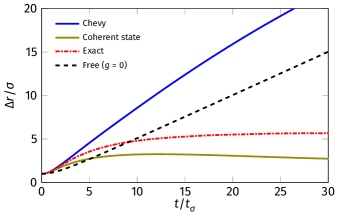
Figure 2: Time evolution of the width $\Delta r$ of the impurity wavepacket. We compare the exact solution (red) to variational results based on a coherent state (yellow) or Chevy Ansatz (blue). The initial width of the wavepacket $\sigma$ sets a characteristic timescale $t_{\sigma}=2m_{\mathrm{I}}\sigma^{2}/\hbar$ and the interaction and boson density $n$ are $g/\Omega=1.5\hbar t_{\sigma}^{-1}$, $\sigma n=0.4$. Free spread obtained for $g=0$ is shown for reference (black).

Since all states are localized in presence of disorder in one dimension, at any finite interaction $g>0$ the wavepacket localizes at $t\to\infty$, i.e., $\psi({\mathbf{r}},t)\to\exp(-|{\mathbf{r}}|/2\xi)$ at large $|{\mathbf{r}}|$ with $\xi$ a localization length. This contrasts with the free case ($g=0$) where the wavepacket spreads indefinitely. A simple observable that distinguishes the two regimes is the width of the wavepacket $\Delta r=\sqrt{\langle({\mathbf{r}}-\langle{\mathbf{r}}\rangle)^{2}\rangle}$. For a localized wavepacket, $\Delta r$ remains finite at all times, while in the free case $\Delta r$ grows linearly with time.

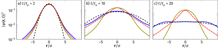
Figure 3: Density profile $|\psi({\mathbf{r}},t)|^{2}$ as function of ${\mathbf{r}}$ of the impurity interacting with a BEC for increasing times $t$. We compare the exact solution (red) to the variational result based on a coherent state (yellow) and Chevy Ansatz (blue). We use $\sigma n=0.4$, $g/\Omega=1.5\hbar t_{\sigma}^{-1}$. The free spread ($g=0$) is shown for reference (black).

We first compare the exact solution of the disorder model to the Chevy Ansatz, which includes for the time-dependent wavefunction $|\Psi^{\mathbf{p}}(t)\rangle$ at most one bosonic excitation [53, 54], i.e.

$$|\Psi^{\mathbf{p}}(t)\rangle {}=\alpha_{0}(t)|{\mathbf{p}}\rangle\otimes|\mathrm{BEC}\rangle$$

$${}+\sum_{{\mathbf{q}}\neq 0}\alpha_{\mathbf{q}}(t)|{\mathbf{p}}+{\mathbf{q}}\rangle\otimes\hat{b}^{\dagger}_{-{\mathbf{q}}}\hat{b}_{0}|\mathrm{BEC}\rangle$$ (9)

where $\alpha_{\mathbf{q}}(t)$ are time-dependent variational parameters; for details see Appendix B.

The time-resolved spreading of the wavepacket is compared to the exact solution in Fig. 2. At short times, we observe good agreement with the exact solution. This is to be expected as, in variational methods, the deviation from the exact solution arises from the iterated projection of the Schrödinger equation and the associated error did not built up at early times. This is also reflected in the evolution of the spatially resolved wavepacket shown in Fig. 3, where the whole density profile is well described by the Chevy Ansatz at short times. Since the Chevy Ansatz specifically relies on including only a small number of excitations, it is most accurate at short times at which the polaron cloud is still developing. However, the Chevy Ansatz breaks down at larger times, and, rather than the localization clearly observed in the exact solution, it predicts the indefinite spread of the wavepacket.

This prompts the search for more involved variational solutions. We consider an Ansatz based on the Lee–Low–Pines (LLP) transformation [55] to transform into the comoving frame of the impurity. In the new frame the impurity momentum ${\mathbf{p}}$ represents the conserved total momentum of the complete system. Impurity operators are hence eliminated and the bosons evolve according to the ${\mathbf{p}}$-dependent Hamiltonian

$$\hat{H}^{\mathrm{BEC}}_{\mathbf{p}}=\dfrac{\big{(}{\mathbf{p}}-\sum_{\mathbf{k}}{\mathbf{k}}\hat{b}_{\mathbf{k}}^{\dagger}\hat{b}_{\mathbf{k}}\big{)}^{2}}{2m_{\mathrm{I}}}+\sum_{\mathbf{k}}\omega_{\mathbf{k}}\hat{b}^{\dagger}_{{\mathbf{k}}}\hat{b}_{\mathbf{k}}+\dfrac{g}{\Omega}\sum_{{\mathbf{k}}{\mathbf{k}}^{\prime}}\hat{b}^{\dagger}_{{\mathbf{k}}}\hat{b}_{{\mathbf{k}}^{\prime}}$$ (10)

which now contains an transformation-induced interaction between bosons. $\Omega$ is the system volume.

The Hamiltonian 10 has been studied using various Ansätze [56, 57, 58, 59, 60, 61, 62, 63]. We approximate the boson wavefunction $|\Phi^{\mathbf{p}}(t)\rangle$ by a product of coherent states,

$$|\Phi^{\mathbf{p}}(t)\rangle=e^{-i\phi^{\mathbf{p}}(t)}e^{\sum_{\mathbf{k}}\beta^{\mathbf{p}}_{\mathbf{k}}(t)\hat{b}^{\dagger}_{\mathbf{k}}-\text{h.c.}}|0\rangle$$ (11)

with variational parameters $\phi^{\mathbf{p}}(t)$ and $\beta_{\mathbf{k}}^{\mathbf{p}}(t)$. By considering this wavefunction, we neglect the possibility of correlations induced between the infinitely massive bosons.

The results for the wavepacket are shown in Figs. 3 and 2. Again, the exact solution is well reproduced at short times, unsurprisingly, since for a state close to the BEC, Eq. 11 reduces to Eq. 9. However, the coherent Ansatz directly addresses one of the shortcomings of the Chevy Ansatz by allowing the description of a large number of bosons excited to small momenta and thus captures localization, although $\xi$ is underestimated.

These examples demonstrate how the exact mapping can help to benchmark variational solutions by providing an exact reference solution of the polaron problem. Indeed both the Chevy and coherent Ansätze can be improved systematically, respectively, by allowing more bosonic excitations [10, 11, 12, 13] or by considering Gaussian states [64] with the mapping allowing to quantify the improvement. This equally applies to other schemes such as non-Gaussian states or quantum Monte-Carlo [65, 66, 67, 68, 69, 70].

V Application to the Anderson transition

A long-standing question in disorder physics is that of the Anderson transition in three dimensions (3D). Unlike in one dimension, where all states are localized, in 3D a mobility edge separates low-energy localized and high-energy extended states [28]. The observation of the mobility edge using the expansion of atomic matter waves through disordered speckle potentials has sparked recent theoretical [71, 72] and experimental interest  [73, 41, 74]. Discrepancies between theory and experiments remain, however, as to the position of the mobility edge [72, 75]. On the theory side, the problem is difficult because it requires going beyond the perturbative weak disorder regime and treating fully the speckle potential, while for experiments it is difficult to prepare a sufficiently narrow energy distribution of the atomic cloud.

The polaron-disorder correspondence can help to obtain further insight. A specific candidate is ⁶Li impurities embedded in ¹³³Cs with $m_{\mathrm{B}}/m_{\mathrm{I}}=22.1$  [76, 77]. In particular, the Li-Cs interaction can be tuned by a Feshbach resonance at 889 G at which the Cs-Cs interaction is small ($a_{\text{CsCs}}\simeq 190a_{0}$). The cloud of impurities expands through the bosonic medium as through a disordered Edwards potential. Theory-wise, one does not have to deal with the speckle potential, and can use the arsenal developed to tackle strongly interacting problems to study the dynamics of the mixture. Nonetheless, the question of the determination of the mobility edge remains an ambitious one. In order to answer it, two key aspects have to be addressed. The first is given by the aforementioned decoherence induced by the finite boson mass. A second constraint is given by the lifetime of the system set, e.g., by three-body loss. This may guide the choice of the system and, for instance, molecular mixtures that feature suppressed three-body loss might prove better candidates despite having lower mass ratios than Li-Cs [78].

VI Conclusion and outlook

We have shown that a generic model of disorder, the Edwards model, is mapped to the problem of a light impurity coupled to a BEC, showing a deep connection between two seemingly very different problems. Our exact mapping has several implications. Experimentally, it offers an alternative setup to investigate the Anderson transition. On the theory side, it can help to develop reliable approximation schemes to describe the Bose polaron problem, while conversely offering an efficient way to bypass the challenging issue of disorder averaging. However, the mapping applies to a much larger class of models. For instance, in the case of a mixture with both interactions and disorder, the mapping can be used to gauge away interactions, reducing it to a single particle problem in presence of two sources of disorder. Another possibility is the realization of more complicated models of disorder, e.g. with long-range correlations, by tuning the boson Hamiltonian.

A promising avenue of research could originate from the field theoretical treatment of the Bose polaron problem. For instance, the Chevy Ansatz is equivalent to a non-selfconsistent $T$-matrix approach [53, 54]. It would be interesting to see how such methods compare to the diagrammatic treatment of disorder, and whether they can be used to shed light on either side of the mapping. Further intriguing applications would be the study of the interplay of disorder and interactions, especially in lower dimensions where many-body methods such as the use of variational matrix product states could help understand thermalization and the spread of entanglement [79, 80, 81, 82]. A recent proposal of a different mapping between disordered systems and interacting semi-metals brings together disorder and many-body physics in a solid state setting  [83]. While our work focusses on cold atom applications, the mapping presented in this work can be extended to other condensed matter systems. Indeed, the crucial ingredient behind the mapping is the absence of boson kinetic energy. Hence, solid state realizations using as a bath a system with flat bands —such as encountered within the quantum Hall effect— are also conceivable.

Appendix A Exact solution of the RKPM

The random Kronig-Penney model (RKPM) is defined by the one-dimensional Hamiltonian

$$\hat{H}_{\mathrm{RKPM}}=-\dfrac{\partial_{x}^{2}}{2m}+g\sum_{i=1}^{N}\delta(x-x_{i}),$$ (12)

describing a single particle in a box of size $L$ with mass $m$ and position $x\in[0,L]$ interacting with fixed random scatterers with a contact potential of strength $g$, with $\hbar$ set to $1$. We consider a given realization of disorder defined by the positions of the $N$ scatterers $x_{i}$, which we chose to be ennumerated as $x_{i}<x_{i+1}$ and note for convenience $x_{0}=0$, $x_{N+1}=L$.

We seek to solve the Schrödinger equation

$$E\psi(x)=-\dfrac{1}{2m}\psi^{\prime\prime}(x)+g\sum_{i=1}^{N}\delta(x-x_{i})\psi(x).$$ (13)

The general solution is found using a standard transfer matrix method, see e.g. Ref.  [48]. We consider only the case of a repulsive scattering potential, $g>0$, for which $E$ is positive, as can been seen by multiplying Eq. 13 by $\psi(x)^{*}$ and integrating over the box. On any subinterval $]x_{i},x_{i+1}[$ the eigenfunctions $\psi(x)$ take the form

$$\psi(x)=A_{i}\sin(kx+\phi_{i})$$ (14)

with $A_{i}$, $\phi_{i}$ an amplitude and a phase and $k\geq 0$ defined by $E=k^{2}/2m$. While $\psi$ is continuous, there is a jump in $\psi^{\prime}$ at each scatterer $x_{i}$,

$$\psi^{\prime}(x_{i}^{+})-\psi^{\prime}(x_{i}^{-})=2mg\psi(x_{i})$$ (15)

as can been seen by integrating Eq. 13 over $[x_{i}^{-},x_{i}^{+}]$.

Constructing the vector $\Psi(x)=(\psi^{\prime}(x),k\psi(x))^{\mathsf{T}}$ indexed by the coordinate $x$, the conditions 14 and 15 can be rewritten as

$$\Psi(x_{i+1}^{-})={} R[k(x_{i+1}-x_{i})]\Psi(x_{i}^{+}), \Psi(x_{i}^{+})={} T\Psi(x_{i}^{-}),$$ (16)

where

$$R(\theta)={} \begin{pmatrix}\cos(\theta)&-\sin(\theta)\\ \sin(\theta)&\cos(\theta)\\ \end{pmatrix}, T={} {}\begin{pmatrix}1&2mg/k\\ 0&1\\ \end{pmatrix}.$$ (17)

Hence, $\Psi(L)=M\Psi(0)$ with

$$M=R[k(L-x_{N})]TR[k(x_{N}-x_{N-1})]\dotsm TR[kx_{1}].$$ (18)

The spectrum is fixed by the boundary conditions; for instance periodic boundary conditions impose $M=1$ or equivalently $\operatorname{Tr}M=2$, as $\det M=1$.

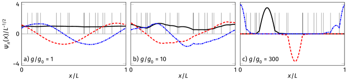
Figure 4: First three eigenstates $\psi_{n=1,2,3}(x)$ of $\hat{H}_{\mathrm{RPKM}}$ for a given realization of disorder for three different interaction strengths $g$, expressed in units of $g_{0}=(2mL)^{-1}$. The ground state wavefunction and the first two excited states are shown in solid black, dashed red and dashdotted blue, respectively. We use periodic boundary conditions in a box of size $L$. The positions of the scatterers $x_{i}$ are represented by grey vertical lines. For weak disorder (a) the wavefunctions closely resemble the solutions of a free particle in a box while at larger interactions (b,c) the eigenstates become localized over distances smaller than the box size.

Once the spectrum is determined, one finds for each eigenvalue the amplitudes and phases $A_{i}$, $\phi_{i}$ defining the eigenstate. Using the continuity of $\psi(x)$ together with Eq. (15) one relates $A_{i+1}$ and $\phi_{i+1}$ to $A_{i}$ and $\phi_{i}$. Thus by recursion $A_{N}$ and $\phi_{N}$ can be expressed as a function of $\phi_{0}$ and $A_{0}$. Finally, a suitable value of $\phi_{0}$ is determined numerically such that the boundary condition is fulfilled, while the amplitudes are fixed by the normalization. As an illustration, we show the first eigenstates thus obtained for a given realization of disorder in Fig. 4.

For attractive interactions ($g<0$), not considered in this article, this method remains valid. However, in this case one also needs to consider eigenstates of negative energy $E=-\kappa^{2}/2m$. On each subinterval, the corresponding wavefunctions then take the form $\psi(x)=A_{i}e^{-\kappa x}+B_{i}e^{\kappa x}$, physically representing states that are exponentially localized about the scatterers. The spectrum and wavefunctions can again be determined by the transfer matrix method.

Appendix B Time-dependent variational method

In this Appendix we briefly review how to determine the time evolution of a ket $|\psi\rangle$ under a Hamiltonian $\hat{H}$ using the variational method; see Refs. [84, 85, 86, 87, 64] for a more in-depth discussion. We first provide a general discussion before applying the formalism to the variational states 9 and 11 introduced in the main text.

We seek for the best approximation of the Schrödinger equation $(i\partial_{t}-\hat{H})|\psi\rangle=0$ with $|\psi\rangle$ being restrained to a variational manifold $\mathcal{M}$. Let us assume that $\mathcal{M}=\{|\psi(z_{i})\rangle,z_{i}\in\mathbb{C}\}$ is parameterized by complex numbers $z_{i}$, with $|\psi(z_{i})\rangle$ an holomorphic funtion of the $z_{i}$-s. Under that assumption, the following three approaches yield the same equations of motions for the variational parameters $z_{i}$. The first is to minimize at all times the norm of the ket $(i\partial_{t}-\hat{H})|\psi\rangle$ with respect to the $\dot{z}_{i}$. The second approach is to extremize the Lagrangian

$$L=\dfrac{i}{2}[\langle\psi|(\partial_{t}|\psi\rangle)-(\partial_{t}\langle\psi|)|\psi\rangle]-\langle\psi|\hat{H}|\psi\rangle$$ (19)

with respect to the variational parameters $(z_{i},\dot{z}_{i})$. The third approach is to project at every time step the Schrödinger equation onto the tangent space to $\mathcal{M}$. We use in practice the last method which we present below.

B.1 Gram matrix formulation

The tangent space to $\mathcal{M}$ at $|\psi\rangle$ is spanned by the vectors

$$|\partial_{i}\psi\rangle=\dfrac{\partial}{\partial z_{i}}|\psi(z)\rangle.$$ (20)

Hence the projected Schrödinger equation is satisfied if and only if for all $i$

$$\langle\partial_{i}\psi|(i\partial_{t}-\hat{H})|\psi\rangle=0.$$ (21)

We now define the energy of the state $E$ and the Gram matrix $G$ using the overlaps of the vectors $|\partial_{i}\psi\rangle$,

$$\begin{aligned} E&=\langle\psi|\hat{H}|\psi\rangle,&E_{j}&=\dfrac{\partial}{\partial z_{j}^{*}}E=\langle\partial_{j}\psi|\hat{H}|\psi\rangle,\end{aligned}$$ (22)

$$G_{ij}=\langle\partial_{i}\psi|\partial_{j}\psi\rangle.$$ (23)

Eq. 21 can then be rewritten as

$$\sum_{j}iG_{ij}\dot{z}_{j}=E_{i}.$$ (24)

In the specific case where $G$ is invertible the equivalent form is

$$i\dot{z}_{i}=\sum_{j}[G^{-1}]_{ij}E_{j}.$$ (25)

Otherwise there is some indeterminacy in the equations of motion, i.e. it is possible to find two different solutions $\dot{z}_{i}$ and $\dot{z}^{\prime}_{i}$ fulfilling Eq. 25 provided $G_{ij}(\dot{z}_{j}-\dot{z}^{\prime}_{j})=0$.

B.2 Application to coherent states

While determining the equations of motion using the Gram formalism for the Chevy Ansatz 9 is straightforward, the case of the coherent state Ansatz is slightly more involved, and we present here the detailed derivation. Indeed, when applying the Gram formalism, one encounters two issues for the coherent Ansatz 11. First, it is not holomorphic (as both $\beta_{\mathbf{k}}$ and $\beta_{\mathbf{k}}^{*}$ appear), and, second, there is no straight-forward equation of motion for the phase, which represents a gauge degree of freedom.

We tackle both issues at once by rather considering the variational state

$$|\beta\rangle{}={} \mathcal{N}e^{\sum_{\mathbf{k}}\beta_{\mathbf{k}}\hat{b}^{\dagger}_{\mathbf{k}}}|0\rangle,$$ (26)

parameterized by the complex numbers $\mathcal{N}$ and $\beta_{\mathbf{k}}$, with $\mathcal{N}$ introduced for normalization. The Ansätze 11 and 26 are completely equivalent provided $\mathcal{N}=e^{-i\phi-\sum_{\mathbf{k}}|\beta_{\mathbf{k}}|^{2}/2}$.

For clarity we drop in this Section the $t$ and ${\mathbf{p}}$ dependencies. We rewrite Eq. 26 by defining the vectors $({\boldsymbol{\beta}})_{\mathbf{k}}=\beta_{\mathbf{k}}$ and $(\hat{\mathbf{b}})_{\mathbf{k}}=\hat{b}_{\mathbf{k}}$, such that $|\beta\rangle=\mathcal{N}e^{\hat{\mathbf{b}}^{\dagger}\cdot{\boldsymbol{\beta}}}|0\rangle$. We also note $S=({\boldsymbol{\beta}})^{\dagger}\cdot{\boldsymbol{\beta}}=\sum_{\mathbf{k}}|\beta_{\mathbf{k}}|^{2}$.

We use the Gram matrix formulation where from the gradients of $|\beta\rangle$,

$$|\partial_{\mathcal{N}}\beta\rangle =\dfrac{\partial}{\partial\mathcal{N}}|\beta\rangle=\dfrac{1}{\mathcal{N}}|\beta\rangle,$$ (27)

$$|\partial_{\mathbf{k}}\beta\rangle =\dfrac{\partial}{\partial\beta_{\mathbf{k}}}|\beta\rangle=\hat{b}_{\mathbf{k}}^{\dagger}|\beta\rangle,$$ (28)

we deduce the Gram matrix [Eq. 23]

$$G=\begin{pmatrix}1&\mathcal{N}{\boldsymbol{\beta}}^{\dagger}\\ \mathcal{N}^{*}{\boldsymbol{\beta}}&|\mathcal{N}|^{2}(\delta+{\boldsymbol{\beta}}\cdot{\boldsymbol{\beta}}^{\dagger})\end{pmatrix}e^{S}.$$ (29)

In the above expression, the first line and column stand for the $\mathcal{N}$ direction, while the rest of the matrix corresponds to the momentum modes labelled by ${\mathbf{k}}$. In the ${\mathbf{k}}$-${\mathbf{k}}$ sector, $\delta$ is understood as the identity matrix and ${\boldsymbol{\beta}}\cdot{\boldsymbol{\beta}}^{\dagger}$ as the matrix with elements $({\boldsymbol{\beta}}\cdot{\boldsymbol{\beta}}^{\dagger})_{{\mathbf{k}},{\mathbf{k}}^{\prime}}=\beta_{\mathbf{k}}\beta_{{\mathbf{k}}^{\prime}}^{*}$. $G$ is invertible with the inverse

$$G^{-1}=\begin{pmatrix}1+S&-\dfrac{1}{\mathcal{N}^{*}}{\boldsymbol{\beta}}^{\dagger}\\ -\dfrac{1}{\mathcal{N}}{\boldsymbol{\beta}}&\dfrac{1}{|\mathcal{N}|^{2}}\delta\end{pmatrix}e^{-S}.$$ (30)

The energy [Eq. 22] is given by

$$E =|\mathcal{N}|^{2}e^{S}E_{0},$$ (31)

with

$$E_{0} =\sum_{\mathbf{k}}(\epsilon_{\mathbf{k}}+\omega_{\mathbf{k}})|\beta_{\mathbf{k}}|^{2}+\dfrac{({\mathbf{p}}-{\mathbf{P}}_{\mathrm{B}}[{\boldsymbol{\beta}}])^{2}}{2m}+\dfrac{g}{\Omega}\Big{|}\sum_{\mathbf{q}}\beta_{\mathbf{q}}\Big{|}^{2}$$ (32)

and ${\mathbf{P}}_{\mathrm{B}}[{\boldsymbol{\beta}}]=\sum_{\mathbf{k}}{\mathbf{k}}|\beta_{\mathbf{k}}|^{2}$ is the total momentum of the bosons. The gradients of $E$ read

$$E_{\mathcal{N}}={} \dfrac{\partial}{\partial\mathcal{N}^{*}}E=\mathcal{N}e^{S}E_{0},$$ (33)

$$E_{\mathbf{k}}={} \dfrac{\partial}{\partial\beta_{\mathbf{k}}^{*}}E=|\mathcal{N}|^{2}e^{S}\bigg{\{}\beta_{\mathbf{k}}E_{0}$$

$${}+\bigg{[}\bigg{(}\epsilon_{\mathbf{k}}+\omega_{\mathbf{k}}-{\mathbf{k}}\cdot\dfrac{{\mathbf{p}}-{\mathbf{P}}_{\mathrm{B}}[{\boldsymbol{\beta}}]}{m}\bigg{)}\beta_{\mathbf{k}}+\dfrac{g}{\Omega}\sum_{\mathbf{q}}\beta_{\mathbf{q}}\bigg{]}\bigg{\}}.$$ (34)

Applying Eq. 25 we obtain

$$i\dot{\beta}_{\mathbf{k}} =\bigg{(}\epsilon_{\mathbf{k}}+\omega_{\mathbf{k}}-{\mathbf{k}}\cdot\dfrac{{\mathbf{p}}-{\mathbf{P}}_{\mathrm{B}}[{\boldsymbol{\beta}}]}{m}\bigg{)}\beta_{\mathbf{k}}+\dfrac{g}{\Omega}\sum_{\mathbf{q}}\beta_{\mathbf{q}},$$ (35)

$$i\dot{\mathcal{N}} =\mathcal{N}\dfrac{{\mathbf{p}}^{2}-{\mathbf{P}}_{\mathrm{B}}[{\boldsymbol{\beta}}]^{2}}{2m}.$$ (36)

From these equations of motion we deduce that $|\mathcal{N}|$ as well as $S$ are constant in time, as expected since the Hamiltonian conserves the number of particles and $S=\langle\beta|\hat{N}|\beta\rangle/\langle\beta|\beta\rangle=N$. Hence the norm of $|\beta\rangle$, $\langle\beta|\beta\rangle=|\mathcal{N}|^{2}e^{S}$, is conserved. We can rewrite $\mathcal{N}=\exp(-S/2)\exp(-i\phi)$ as

$$\dot{\phi}=\dfrac{{\mathbf{p}}^{2}-{\mathbf{P}}_{\mathrm{B}}[{\boldsymbol{\beta}}]^{2}}{2m_{\mathrm{I}}}.$$ (37)

Using this new notation, 26 is exactly equivalent to 11. The equations of motion thus obtained are the same as those present in the literature, see e.g. Ref. [58].

References

- Landau and Pekar [1948] L. Landau and S. Pekar, Effective mass of a polaron, J. Exp. Theor. Phys. 18, 419 (1948).
- Duke and Mahan [1965] C. B. Duke and G. D. Mahan, Phonon-Broadened Impurity Spectra. I. Density of States, Phys. Rev. 139, A1965 (1965).
- Alexandrov and Mott [1995] A. S. Alexandrov and N. F. Mott, Polarons and Bipolarons (World Scientific, Singapore, 1995).
- Baym and Pethick [1991] G. Baym and C. Pethick, Landau Fermi-Liquid Theory: Concepts and Applications (Wiley-VCH, New York, 1991).
- Gershenson et al. [2006] M. E. Gershenson, V. Podzorov, and A. F. Morpurgo, Colloquium: Electronic transport in single-crystal organic transistors, Rev. Mod. Phys. 78, 973 (2006).
- Dagotto [1994] E. Dagotto, Correlated electrons in high-temperature superconductors, Rev. Mod. Phys. 66, 763 (1994).
- Devreese and Alexandrov [2009] J. T. Devreese and A. S. Alexandrov, Fröhlich polaron and bipolaron: recent developments, Rep. Prog. Phys. 72, 066501 (2009).
- Volosniev et al. [2015] A. G. Volosniev, H.-W. Hammer, and N. T. Zinner, Real-time dynamics of an impurity in an ideal Bose gas in a trap, Phys. Rev. A 92, 023623 (2015).
- García-March et al. [2016] M. A. García-March, A. S. Dehkharghani, and N. T. Zinner, Entanglement of an impurity in a few-body one-dimensional ideal Bose system, J. Phys. B 49, 075303 (2016).
- Levinsen et al. [2015] J. Levinsen, M. M. Parish, and G. M. Bruun, Impurity in a Bose-Einstein Condensate and the Efimov Effect, Phys. Rev. Lett. 115, 125302 (2015).
- Yoshida et al. [2018] S. M. Yoshida, S. Endo, J. Levinsen, and M. M. Parish, Universality of an Impurity in a Bose-Einstein Condensate, Phys. Rev. X 8, 011024 (2018).
- Shi et al. [2018a] Z.-Y. Shi, S. M. Yoshida, M. M. Parish, and J. Levinsen, Impurity-Induced Multibody Resonances in a Bose Gas, Phys Rev. Lett. 121, 243401 (2018a).
- Levinsen et al. [2021] J. Levinsen, L. A. P. Ardila, S. M. Yoshida, and M. M. Parish, Quantum Behavior of a Heavy Impurity Strongly Coupled to a Bose Gas, Phys. Rev. Lett. 127, 033401 (2021).
- Dehkharghani et al. [2018] A. S. Dehkharghani, A. G. Volosniev, and N. T. Zinner, Coalescence of Two Impurities in a Trapped One-dimensional Bose Gas, Phys. Rev. Lett. 121, 080405 (2018).
- Jager et al. [2020] J. Jager, R. Barnett, M. Will, and M. Fleischhauer, Strong-coupling Bose polarons in one dimension: Condensate deformation and modified Bogoliubov phonons, Phys. Rev. Research 2, 033142 (2020).
- Dzsotjan et al. [2020] D. Dzsotjan, R. Schmidt, and M. Fleischhauer, Dynamical Variational Approach to Bose Polarons at Finite Temperatures, Phys. Rev. Lett. 124, 223401 (2020).
- Guenther et al. [2021] N.-E. Guenther, R. Schmidt, G. M. Bruun, V. Gurarie, and P. Massignan, Mobile impurity in a Bose-Einstein condensate and the orthogonality catastrophe, Phys. Rev. A 103, 013317 (2021).
- Massignan et al. [2021] P. Massignan, N. Yegovtsev, and V. Gurarie, Universal Aspects of a Strongly Interacting Impurity in a Dilute Bose Condensate, Phys. Rev. Lett. 126, 123403 (2021).
- Isaule et al. [2021] F. Isaule, I. Morera, P. Massignan, and B. Juliá-Díaz, Renormalization-group study of Bose polarons, Phys. Rev. A 104, 023317 (2021).
- Schmidt and Enss [2021] R. Schmidt and T. Enss, Self-stabilized Bose polarons, arXiv:2102.13616 [cond-mat.quant-gas] (2021).
- Franchini et al. [2021] C. Franchini, M. Reticcioli, M. Setvin, and U. Diebold, Polarons in materials, Nat. Rev. Mater. (2021).
- Seetharam et al. [2021] K. Seetharam, Y. Shchadilova, F. Grusdt, M. B. Zvonarev, and E. Demler, Dynamical Quantum Cherenkov Transition of Fast Impurities in Quantum Liquids, Phys. Rev. Lett. 127, 185302 (2021).
- Hu et al. [2016] M.-G. Hu, M. J. Van de Graaff, D. Kedar, J. P. Corson, E. A. Cornell, and D. S. Jin, Bose Polarons in the Strongly Interacting Regime, Phys. Rev. Lett. 117, 055301 (2016).
- Jørgensen et al. [2016] N. B. Jørgensen, L. Wacker, K. T. Skalmstang, M. M. Parish, J. Levinsen, R. S. Christensen, G. M. Bruun, and J. J. Arlt, Observation of Attractive and Repulsive Polarons in a Bose-Einstein Condensate, Phys. Rev. Lett. 117, 055302 (2016).
- Yan et al. [2020] Z. Z. Yan, Y. Ni, C. Robens, and M. W. Zwierlein, Bose polarons near quantum criticality, Science 368, 190 (2020).
- Peña Ardila et al. [2019] L. A. Peña Ardila, N. B. Jørgensen, T. Pohl, S. Giorgini, G. M. Bruun, and J. J. Arlt, Analyzing a Bose polaron across resonant interactions, Phys. Rev. A 99, 063607 (2019).
- Skou et al. [2021] M. G. Skou, T. G. Skov, N. B. Jørgensen, K. K. Nielsen, A. Camacho-Guardian, T. Pohl, G. M. Bruun, and J. J. Arlt, Non-equilibrium quantum dynamics and formation of the Bose polaron, Nat. Phys. 17, 2005.00424 (2021).
- Anderson [1958] P. W. Anderson, Absence of Diffusion in Certain Random Lattices, Phys. Rev. 109, 1492 (1958).
- Sharvin and Sharvin [1981] D. Y. Sharvin and Y. V. Sharvin, Magnetic-flux quantization in a cylindrical film of a normal metal, J. Exp. Theor. Phys. Lett. 34, 272 (1981).
- Pannetier et al. [1984] B. Pannetier, J. Chaussy, R. Rammal, and P. Gandit, Magnetic Flux Quantization in the Weak-Localization Regime of a Nonsuperconducting Metal, Phys. Rev. Lett. 53, 718 (1984).
- Kuga and Ishimaru [1984] Y. Kuga and A. Ishimaru, Retroreflectance from a dense distribution of spherical particles, J. Opt. Soc. Am. A 1, 831 (1984).
- Wolf and Maret [1985] P.-E. Wolf and G. Maret, Weak Localization and Coherent Backscattering of Photons in Disordered Media, Phys. Rev. Lett. 55, 2696 (1985).
- Albada and Lagendijk [1985] M. P. V. Albada and A. Lagendijk, Observation of Weak Localization of Light in a Random Medium, Phys. Rev. Lett. 55, 2692 (1985).
- Fleishman and Anderson [1980] L. Fleishman and P. W. Anderson, Interactions and the Anderson transition, Phys. Rev. B 21, 2366 (1980).
- Basko et al. [2006] D. M. Basko, I. L. Aleiner, and B. L. Altshuler, Metal insulator transition in a weakly interacting many-electron system with localized single-particle states, Ann. Phys. 321, 1126 (2006).
- Oganesyan and Huse [2007] V. Oganesyan and D. A. Huse, Localization of interacting fermions at high temperature, Phys. Rev. B 75, 155111 (2007).
- Nandkishore and Huse [2015] R. Nandkishore and D. A. Huse, Many-Body Localization and Thermalization in Quantum Statistical Mechanics, Annu. Rev. Condens. Matter Phys. 6, 15 (2015).
- Dalichaouch et al. [1991] R. Dalichaouch, J. P. Armstrong, S. Schultz, P. M. Platzman, and S. L. McCall, Microwave localization by two-dimensional random scattering, Nature 354, 53 (1991).
- Ye et al. [1992] L. Ye, G. Cody, M. Zhou, P. Sheng, and A. N. Norris, Observation of bending wave localization and quasi mobility edge in two dimensions, Phys. Rev. Lett. 69, 3080 (1992).
- Billy et al. [2008] J. Billy, V. Josse, Z. Zuo, A. Bernard, B. Hambrecht, P. Lugan, D. Clément, L. Sanchez-Palencia, P. Bouyer, and A. Aspect, Direct observation of Anderson localization of matter waves in a controlled disorder, Nature 453, 891 (2008).
- Jendrzejewski et al. [2012] F. Jendrzejewski, A. Bernard, K. Müller, P. Cheinet, V. Josse, M. Piraud, L. Pezzé, L. Sanchez-Palencia, A. Aspect, and P. Bouyer, Three-dimensional localization of ultracold atoms in an optical disordered potential, Nat. Phys. 8, 398 (2012).
- Eckardt and Anisimovas [2015] A. Eckardt and E. Anisimovas, High-frequency approximation for periodically driven quantum systems from a Floquet-space perspective, New J. Phys. 17, 093039 (2015).
- Hainaut et al. [2019] C. Hainaut, A. Rançon, J.-F. Clément, I. Manai, P. Szriftgiser, D. Delande, J. C. Garreau, and R. Chicireanu, Experimental realization of an ideal Floquet disordered system, New J. Phys. 21, 035008 (2019).
- Fishman et al. [1982] S. Fishman, D. R. Grempel, and R. E. Prange, Chaos, Quantum Recurrences, and Anderson Localization, Phys. Rev. Lett. 49, 509 (1982).
- S. F. Edwards [1958] S. F. Edwards, A New Method for the Evaluation of Electric Conductivity in Metals, Phil. Mag. 3, 1020 (1958).
- Akkermans and Montambaux [2007] E. Akkermans and G. Montambaux, Mesoscopic Physics of Electrons and Photons (Cambridge University Press, Cambridge, 2007).
- Lax and Phillips [1958] M. Lax and J. C. Phillips, One-Dimensional Impurity Bands, Phys. Rev. 110, 41 (1958).
- Nieuwenhuizen [1983] T. Nieuwenhuizen, Exact electronic spectra and inverse localization lengths in one-dimensional random systems: I. Random alloy, liquid metal and liquid alloy, Physica A 120, 468 (1983).
- Gavish and Castin [2005] U. Gavish and Y. Castin, Matter-Wave Localization in Disordered Cold Atom Lattices, Phys. Rev. Lett. 95, 020401 (2005).
- Paredes et al. [2005] B. Paredes, F. Verstraete, and J. I. Cirac, Exploiting Quantum Parallelism to Simulate Quantum Random Many-Body Systems, Phys. Rev. Lett. 95, 140501 (2005).
- Grover and Fisher [2014] T. Grover and M. P. A. Fisher, Quantum disentangled liquids, J. Stat. Mech: Theory Exp. 2014, 10010 (2014).
- Berne and Pecora [1976] B. J. Berne and R. Pecora, Dynamic Light Scattering with Applications to Chemistry, Biology and Physics (John Wiley, New York, 1976).
- Rath and Schmidt [2013] S. P. Rath and R. Schmidt, Field-theoretical study of the Bose polaron, Phys. Rev. A 88, 053632 (2013).
- Li and Das Sarma [2014] W. Li and S. Das Sarma, Variational study of polarons in Bose-Einstein condensates, Phys. Rev. A 90, 013618 (2014).
- Lee et al. [1953] T. D. Lee, F. E. Low, and D. Pines, The Motion of Slow Electrons in a Polar Crystal, Phys. Rev. 90, 297 (1953).
- Shashi et al. [2014] A. Shashi, F. Grusdt, D. A. Abanin, and E. Demler, Radio-frequency spectroscopy of polarons in ultracold Bose gases, Phys. Rev. A 89, 053617 (2014).
- Grusdt et al. [2014] F. Grusdt, A. Shashi, D. Abanin, and E. Demler, Bloch oscillations of bosonic lattice polarons, Phys. Rev. A 90, 063610 (2014).
- Shchadilova et al. [2016] Y. E. Shchadilova, R. Schmidt, F. Grusdt, and E. Demler, Quantum Dynamics of Ultracold Bose Polarons, Phys. Rev. Lett. 117, 113002 (2016).
- Kain and Ling [2017] B. Kain and H. Y. Ling, Hartree-Fock treatment of Fermi polarons using the Lee-Low-Pine transformation, Phys. Rev. A 96, 033627 (2017).
- Nakano et al. [2017] E. Nakano, H. Yabu, and K. Iida, Bose-Einstein-condensate polaron in harmonic trap potentials in the weak-coupling regime: Lee-Low-Pines-type approach, Phys. Rev. A 95, 023626 (2017).
- Yakaboylu et al. [2018] E. Yakaboylu, B. Midya, A. Deuchert, N. Leopold, and M. Lemeshko, Theory of the rotating polaron: Spectrum and self-localization, Phys. Rev. B 98, 224506 (2018).
- Drescher et al. [2019] M. Drescher, M. Salmhofer, and T. Enss, Real-space dynamics of attractive and repulsive polarons in Bose-Einstein condensates, Phys. Rev. A 99, 023601 (2019).
- Drescher et al. [2020] M. Drescher, M. Salmhofer, and T. Enss, Theory of a resonantly interacting impurity in a Bose-Einstein condensate, Phys. Rev. Res. 2, 032011 (2020).
- Shi et al. [2018b] T. Shi, E. Demler, and J. Ignacio Cirac, Variational study of fermionic and bosonic systems with non-Gaussian states: Theory and applications, Ann. Phys. 390, 245 (2018b).
- Ardila and Giorgini [2015] L. A. P. Ardila and S. Giorgini, Impurity in a Bose-Einstein condensate: Study of the attractive and repulsive branch using quantum Monte Carlo methods, Phys. Rev. A 92, 033612 (2015).
- Ardila and Giorgini [2016] L. A. P. n. Ardila and S. Giorgini, Bose polaron problem: Effect of mass imbalance on binding energy, Phys. Rev. A 94, 063640 (2016).
- Grusdt et al. [2017] F. Grusdt, G. E. Astrakharchik, and E. Demler, Bose polarons in ultracold atoms in one dimension: beyond the Fröhlich paradigm, New J. Phys. 19, 103035 (2017).
- Parisi and Giorgini [2017] L. Parisi and S. Giorgini, Quantum Monte Carlo study of the Bose-polaron problem in a one-dimensional gas with contact interactions, Phys. Rev. A 95, 023619 (2017).
- Akaturk and Tanatar [2019] E. Akaturk and B. Tanatar, Two-dimensional Bose polaron using diffusion Monte Carlo method, Int. J. Mod. Phys. B 33, 1950238 (2019).
- Vlietinck et al. [2015] J. Vlietinck, W. Casteels, K. V. Houcke, J. Tempere, J. Ryckebusch, and J. T. Devreese, Diagrammatic Monte Carlo study of the acoustic and the Bose–Einstein condensate polaron, New Journal of Physics 17, 033023 (2015).
- Delande and Orso [2014] D. Delande and G. Orso, Mobility Edge for Cold Atoms in Laser Speckle Potentials, Phys. Rev. Lett. 113, 060601 (2014).
- Pasek et al. [2017] M. Pasek, G. Orso, and D. Delande, Anderson Localization of Ultracold Atoms: Where is the Mobility Edge?, Phys. Rev. Lett. 118, 170403 (2017).
- Kondov et al. [2011] S. S. Kondov, W. R. McGehee, J. J. Zirbel, and B. DeMarco, Three-Dimensional Anderson Localization of Ultracold Matter, Science 334, 66 (2011).
- Semeghini et al. [2015] G. Semeghini, M. Landini, P. Castilho, S. Roy, G. Spagnolli, A. Trenkwalder, M. Fattori, M. Inguscio, and G. Modugno, Measurement of the mobility edge for 3D Anderson localization, Nat. Phys. 11, 554 (2015).
- Cherroret et al. [2021] N. Cherroret, T. Scoquart, and D. Delande, Coherent multiple scattering of out-of-equilibrium interacting Bose gases, Ann. Phys. 2021, 168543 (2021).
- Petrov and Werner [2015] D. S. Petrov and F. Werner, Three-body recombination in heteronuclear mixtures at finite temperature, Phys. Rev. A 92, 022704 (2015).
- Häfner et al. [2017] S. Häfner, J. Ulmanis, E. D. Kuhnle, Y. Wang, C. H. Greene, and M. Weidemüller, Role of the intraspecies scattering length in the Efimov scenario with large mass difference, Phys. Rev. A 95, 062708 (2017).
- Ciamei et al. [2021] A. Ciamei, S. Finelli, M. Inguscio, A. Trenkwalder, and M. Zaccanti, Ultracold 6Li-53Cr Fermi mixtures with tunable interactions, Bulletin of the American Physical Society (2021).
- Bardarson et al. [2012] J. H. Bardarson, F. Pollmann, and J. E. Moore, Unbounded Growth of Entanglement in Models of Many-Body Localization, Phys. Rev. Lett. 109, 017202 (2012).
- Serbyn et al. [2013] M. Serbyn, Z. Papić, and D. A. Abanin, Universal Slow Growth of Entanglement in Interacting Strongly Disordered Systems, Phys. Rev. Lett. 110, 260601 (2013).
- Agarwal et al. [2017] K. Agarwal, E. Altman, E. Demler, S. Gopalakrishnan, D. A. Huse, and M. Knap, Rare-region effects and dynamics near the many-body localization transition, Ann. Phys. (Berl.) 529, 1600326 (2017).
- Schreiber et al. [2015] M. Schreiber, S. S. Hodgman, P. Bordia, H. P. Lüschen, M. H. Fischer, R. Vosk, E. Altman, U. Schneider, and I. Bloch, Observation of many-body localization of interacting fermions in a quasirandom optical lattice, Science 349, 842 (2015).
- Sun and Syzranov [2021] S. Sun and S. Syzranov, Equivalence of interacting semimetals and low-density many-body systems to single-particle systems with quenched disorder, arXiv:2104.02720 [cond-mat.mes-hall] (2021).
- A.D. McLachlan [1964] A.D. McLachlan, A variational solution of the time-dependent Schrodinger equation, Molecular Physics 8, 39 (1964).
- Kramer and Saraceno [1981] P. Kramer and M. Saraceno, Geometry of the Time-Dependent Variational Principle in Quantum Mechanics (Lecture Notes in Physics) (Springer, Berlin, Heidelberg, 1981).
- Basile and Elser [1995] A. G. Basile and V. Elser, Equations of motion for superfluids, Phys. Rev. E 51, 5688 (1995).
- Haegeman et al. [2011] J. Haegeman, J. I. Cirac, T. J. Osborne, I. Pižorn, H. Verschelde, and F. Verstraete, Time-Dependent Variational Principle for Quantum Lattices, Phys. Rev. Lett. 107, 070601 (2011).