Time reversal symmetry protected chaotic fixed point in the quench dynamics of a topological $p$-wave superfluid

Abstract

We study the quench dynamics of a topological $p$-wave superfluid with two competing order parameters, $\Delta_{\pm}(t)$. When the system is prepared in the $p+ip$ ground state and the interaction strength is quenched, only $\Delta_{+}(t)$ is nonzero. However, we show that fluctuations in the initial conditions result in the growth of $\Delta_{-}(t)$ and chaotic oscillations of both order parameters. We term this behavior phase III’. In addition, there are two other types of late time dynamics – phase I where both order parameters decay to zero and phase II where $\Delta_{+}(t)$ asymptotes to a nonzero constant while $\Delta_{-}(t)$ oscillates near zero. Although the model is nonintegrable, we are able to map out the exact phase boundaries in parameter space. Interestingly, we find phase III’ is unstable with respect to breaking the time reversal symmetry of the interaction. When one of the order parameters is favored in the Hamiltonian, the other one rapidly vanishes and the previously chaotic phase III’ is replaced by the Floquet topological phase III that is seen in the integrable chiral $p$-wave model.

I Introduction

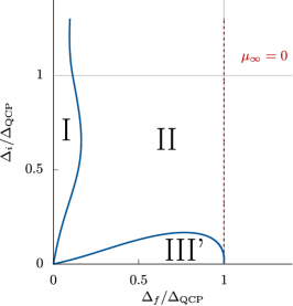
Figure 1: Exact quantum quench phase diagram of a $p$-wave superfluid. Each point represents an interaction quench from a slightly perturbed $p+ip$ ground state, where $\Delta_{i}$ and $\Delta_{f}$ are the ground state $p$-wave order parameter amplitudes for the initial and final couplings. In equilibrium, there is a quantum critical point at $\Delta=\Delta_{\mathrm{QCP}}$, which separates the topologically nontrivial BCS ($\Delta<\Delta_{\mathrm{QCP}}$) and topologically trivial BEC ($\Delta>\Delta_{\mathrm{QCP}}$) ground states. The red dashed line is the nonequilibrium extension of this critical point. Away from equilibrium, the system exhibits competing $p\pm ip$ orders each with its own time dependent complex amplitude $\Delta_{\pm}(t)$. In phase I, both amplitudes decay to zero due to dephasing, $\lvert\Delta_{\pm}(t)\rvert\rightarrow 0$. In phase II, the $p+ip$ amplitude has damped oscillations and decays to a nonzero constant, while the $p-ip$ one shows small oscillations. In phase III’, both amplitudes grow and exhibit chaotic dynamics.

Figure 2: A diagram illustrating the effect of time reversal symmetry breaking on $p$-wave superfluid dynamics. $G_{\pm}$ are coupling constants of the $p+ip$ and $p-ip$ interaction terms. The symmetry is broken whenever $G_{+}\neq G_{-}$. In much of this paper we study a time reversal invariant superfluid where $G_{+}=G_{-}$. For a chiral $p$-wave superfluid either $G_{-}=0$ or $G_{+}=0$ leading to a quench phase diagram which differs from Fig. 1 by a replacement of phase III’ with a Floquet topological phase III. For $G_{+}\neq G_{-}$, we find that the pairing amplitude associated with the weaker channel rapidly vanishes. The amplitude of the stronger channel survives to late times and its dynamics resemble the quench dynamics of the chiral $p$-wave superfluid. Phase III’ is thus an unstable fixed point protected by time reversal symmetry.

One of the most significant problems challenging our modern understanding of physics is the characterization of many body systems that are far from equilibrium. The extent to which conventional tools and frameworks such as the Landau-Ginzburg-Wilson theory, topological order, and universality remain valid descriptions of systems out of equilibrium is not readily understood. Fortunately, in recent years, there has been great progress in the development of both experimental and theoretical tools that allow us to begin answering such questions.

Advances in ultra cold atomic systems [1, 2, 3, 4, 5, 6, 7, 8, 9, 10, 11, 12, 13, 14], quantum devices [15, 16, 17, 18, 19], and high frequency pump-probe spectroscopy [20, 21, 22, 23, 24, 25, 26] have provided a platform for simulating quantum many body dynamics. These experiments have shown great promise in their ability to both guide and verify our understanding of thermalization and nonequilibrium dynamical phases. There have also been numerical and analytical techniques developed for studying the dynamics of systems far from equilibrium [27, 28, 29, 30, 31, 32, 33, 34, 35] as well as efforts at defining a notion of nonequilibrium topology [36, 37, 38, 39, 40, 41, 42, 43, 44, 45, 46, 47, 48, 49, 50].

In this work, we characterize the late time quantum quench dynamics of a topological 2D $p$-wave superfluid with two competing order parameters [51, 52]. Such a system can, in principle, be realized in the context of cold atomic gases where an attractive interaction between identical fermions can be tuned through a Feshbach resonance [53, 54, 10]. The system is expected to have $p+ip$ and $p-ip$ ground states, where $p\pm ip$ refers to the symmetry of the superfluid order parameter: $\Delta_{\mathbf{p}}=(p^{x}\mp ip^{y})\Delta_{\pm}$, $p^{x}$ and $p^{y}$ are the $x$ and $y$ components of the 2D momentum $\mathbf{p}$, and $\Delta_{+}$ and $\Delta_{-}$ are the $p+ip$ and $p-ip$ pairing amplitudes, respectively. In the $p+ip$ ground state $\Delta_{-}=0$ while in the $p-ip$ ground state $\Delta_{+}=0$. Remarkably, the ground state can be tuned across a quantum phase transition by varying the chemical potential, $\mu$, of the system. For $\mu<0$, the system is in the topologically trivial strong pairing BEC phase while for $\mu>0$ it is in the topologically nontrivial weak pairing BCS phase. The transition occurs at the quantum critical point $\mu=0$ where the ground state pairing amplitude takes on the value $\Delta_{\mathrm{QCP}}$, see Sec. II.1 for details.

Unfortunately, attempts to experimentally realize such a gas have proven difficult due to the short lifetimes before losses induced by three-body processes destabilize the gas [54]. However, the ability to tune interactions via resonances has led to the consideration of using out of equilibrium dynamics as a means to induce metastable phases. In particular, it was argued that from a weakly paired $p+ip$ or, equivalently, $p-ip$ ground state it is possible to induce a Floquet topological superfluid by a sudden interaction quench in the time before the instability occurs [37].

Though this seems promising, a deeper understanding of the nonequilibrium $p$-wave superfluid is necessary before conclusions can be drawn. The degree of fine tuning required to realize this behavior has not been understood and, naturally, the question arises as to whether these dynamics are stable against small fluctuations around the $p+ip$ ground state due to, e.g., additional interactions, finite temperature, or coupling to the environment. In other words, do deviations from the $p+ip$ ground state affect the existence of this phase? Instabilities in oscillatory dynamical phases have been shown to occur in similar models of superfluids [55, 56]. There, the instabilities are driven by spatial, thermal or quantum fluctuations.

Through the use of analytical techniques and numerical simulations we are able to map out the entire interaction quench phase diagram of the $p$-wave superfluid, see Fig. 1. We start in a slightly perturbed $p+ip$ ground state with initial superfluid interaction strength $G_{i}$ and then abruptly change the interaction to $G_{f}$. The ground state value of the pairing amplitude $\Delta_{0,+}(G)$ is a monotonic function of the interaction strength $G$ and we find it convenient to represent the $G_{i}\rightarrow G_{f}$ quench as a point with coordinates $(\Delta_{i},\Delta_{f})$ in the phase diagram, where $\Delta_{i}=\Delta_{0,+}(G_{i})$ and $\Delta_{f}=\Delta_{0,+}(G_{f})$. By symmetry, the phase diagram for quenches from a slightly perturbed $p-ip$ ground state is obtained via a simple interchange of $\Delta_{+}$ and $\Delta_{-}$.

Unfortunately, we find that small fluctuations completely destroy the Floquet topological superfluid. The quench phase diagram of the $p$-wave superfluid consists of three nonequilibrium phases classified according to the late time dynamics of the two order parameter pairing amplitudes $\Delta_{+}(t)$ and $\Delta_{-}(t)$. In phase I, both amplitudes decay to zero due to dephasing. In phase II, $\Delta_{+}(t)$ has damped oscillations and decays to a nonzero constant while $\Delta_{-}(t)$ stays small and shows persistent nonperiodic oscillations. In phase III’, the two order parameter amplitudes grow and exhibit chaotic oscillations. Surprisingly, even though the $p$-wave Hamiltonian is nonintegrable, we find an analytic description of the phase boundaries that is consistent with our numerical simulations. The resulting quantum quench phase diagram is shown in Fig. 1. The quench phase diagram of the chiral $p$-wave model studied in Ref. 36 is the same except our new chaotic and nontopological phase III’ is replaced with the Floquet topological phase III .

To gain insight into the properties of phase III’, we consider the limit $\Delta_{i}\rightarrow 0$, which corresponds to the horizontal axis of the quench phase diagram in Fig. 1. In this case, the initial state is close to the ground state of a free Fermi gas (the normal state) and we can understand the short time pairing dynamics by performing a linear stability analysis around this state. We find that both amplitudes grow as $\Delta_{\pm}(t)\propto e^{\gamma t}$ with the same rate $\gamma$. For small interaction strengths, $\gamma=\Delta_{f}\sqrt{2\epsilon_{F}}$, where $\epsilon_{F}$ is the Fermi energy. As we increase $\Delta_{f}$ moving towards the phase III’–II transition point along the $\Delta_{i}=0$ line, $\gamma$ decreases until it vanishes at the transition becoming purely imaginary afterwards. We find that the transition point is at $\Delta_{f}=\Delta_{\mathrm{QCP}}$. Thus, three transitions occur at the same value of the ground state pairing amplitude $\Delta_{f}=\Delta_{\mathrm{QCP}}$: (i) the equilibrium BCS–BEC quantum phase transition, (ii) the transition between nonequilibrium phases III’ and II for $\Delta_{i}=0$ and (iii) change in the stability of the normal state with respect to superfluid interactions. A rather remarkable byproduct of this analysis is that the equilibrium BCS–BEC quantum phase transition can be defined solely in terms of the stability of the normal state – the BCS phase is when the normal state is dynamically unstable and the BEC phase is when it is stable.

Finally, we study the effects of time reversal symmetry breaking on the late time dynamics of the quenched $p$-wave superfluid. The $p$-wave interactions can be divided into $p+ip$ and $p-ip$ interaction channels. Time reversal invariance requires that interaction strengths of the two channels be equal to each other, $G_{+}=G_{-}=G$. This is the model we consider throughout this paper (except Sec. V) and whose quench phase diagram appears in Fig. 1. The chiral $p$-wave model has either $G_{+}=0$ or $G_{-}=0$ and accordingly there is only one nonzero pairing amplitude, $\Delta_{+}$ or $\Delta_{-}$. To better understand the effect of time reversal symmetry breaking, we consider the situation when both couplings are nonzero and unequal, $G_{+}\neq G_{-}$, in Sec. V. We find that the pairing amplitude associated with the weaker channel rapidly vanishes while the amplitude of the stronger channel survives to late times regardless of the initial state, i.e., the stronger channel always wins. These late time dynamics closely resemble the quench dynamics of a chiral $p$-wave superfluid, though for a modified set of quench parameters. The $p$-wave phase III’ therefore represents an unstable fixed point protected by time reversal symmetry, see Fig. 2. As soon as we make $G_{+}\neq G_{-}$, the dynamics that previously lead to phase III’ take the system into the Floquet phase III of Ref. 36. This result indicates that it is still possible to observe a quench induced Floquet topological superfluid phase provided the time reversal symmetry of the interaction term is explicitly broken.

II Equilibrium properties of the BCS Hamiltonian

The simplest realistic 2-D $p$-wave BCS Hamiltonian is given by [53]

$$\hat{H}=\sum_{\mathbf{k}}\frac{k^{2}}{m}\hat{c}^{\dagger}_{\mathbf{k}}\hat{c}_{\mathbf{k}}-\frac{2G}{m}\sum_{\mathbf{p},\mathbf{k},\mathbf{q}}\mathbf{k}\cdot\mathbf{q}\hat{c}^{\dagger}_{\frac{\mathbf{p}}{2}+\mathbf{k}}\hat{c}^{\dagger}_{\frac{\mathbf{p}}{2}-\mathbf{k}}\hat{c}_{\frac{\mathbf{p}}{2}-\mathbf{q}}\hat{c}_{\frac{\mathbf{p}}{2}+\mathbf{q}}$$ (1)

where the operator $\hat{c}^{\dagger}_{\mathbf{k}}$ ($\hat{c}_{\mathbf{k}}$) creates (annihilates) a spinless fermion with momentum $\mathbf{k}$ and $G>0$ is the dimensionless BCS coupling. We will focus only on the interaction terms with $\mathbf{p}=0$, i.e. the reduced BCS model, and neglect the pair breaking terms, $\mathbf{p}\neq 0$. This approximation is valid away from equilibrium as long as the characteristic timescale of the dynamics is less than the time for pair breaking processes to occur. We expect this to be the case away from the quantum critical point (and its nonequilibrium extension) where the chemical potential, $\mu~{}(\mu_{\infty})$, vanishes [58].

It is convenient to express Eq. (1) in terms of Anderson pseudospins defined through the relationships [59]

$$\begin{split}\hat{s}_{\mathbf{k}}^{z}&=\frac{1}{2}\left(\hat{c}^{\dagger}_{\mathbf{k}}\hat{c}_{\mathbf{k}}+\hat{c}^{\dagger}_{\mathbf{-k}}\hat{c}_{\mathbf{-k}}-1\right),\\ \hat{s}_{\mathbf{k}}^{+}&=\hat{c}^{\dagger}_{\mathbf{k}}\hat{c}^{\dagger}_{\mathbf{-k}},\\ \hat{s}_{\mathbf{k}}^{-}&=\hat{c}_{\mathbf{-k}}\hat{c}_{\mathbf{k}}.\end{split}$$ (2)

With this replacement, the reduced ($\mathbf{p}=0$) Hamiltonian becomes

$$\hat{H}=\sum_{\mathbf{k}}^{\prime}k^{2}\hat{s}^{z}_{\mathbf{k}}-2G\sum_{\mathbf{k},\mathbf{q}}^{\prime}\mathbf{k}\cdot\mathbf{q}\hat{s}_{\mathbf{k}}^{+}\hat{s}_{\mathbf{q}}^{-}$$ (3)

where, without loss of generality, we have set $m=1$. The primed sums indicate that the momenta are restricted to the upper half plane so that $\mathbf{k}=\{k^{x}\in\mathbb{R},k^{y}\geq 0\}$ and double counting is avoided. It is easily verified that the pseudospins satisfy the usual commutation relations $\left[\hat{s}_{\mathbf{k}}^{a},\hat{s}_{\mathbf{q}}^{b}\right]=i\delta_{\mathbf{k},\mathbf{q}}\epsilon^{abc}\hat{s}_{\mathbf{k}}^{c}$.

In a mean-field treatment, the Hamiltonian in Eq. (3) can be rewritten as

$$\begin{split}\hat{H}_{MF}=\sum_{\mathbf{k}}^{\prime}k^{2}\hat{s}^{z}_{\mathbf{k}}&+\sum_{\mathbf{k}}^{\prime}k\left(e^{-i\phi_{\mathbf{k}}}\Delta_{+}+e^{+i\phi_{\mathbf{k}}}\Delta_{-}\right)\hat{s}_{\mathbf{k}}^{+}\\ &+\sum_{\mathbf{k}}^{\prime}k\left(e^{+i\phi_{\mathbf{k}}}\Delta^{*}_{+}+e^{-i\phi_{\mathbf{k}}}\Delta^{*}_{-}\right)\hat{s}_{\mathbf{k}}^{-}\end{split}$$ (4)

where

$$\Delta_{\pm}\equiv-G\sum_{\mathbf{k}}ke^{\pm i\phi_{\mathbf{k}}}\langle\hat{s}_{\mathbf{k}}^{-}\rangle$$ (5)

is the pairing amplitude associated with the $p\pm ip$ superfluid order parameter, $\phi_{\mathbf{k}}$ is the polar angle in the $k^{x},k^{y}$ plane, and the expectation values are taken with respect to the many-body wavefunction of the system.

The Heisenberg equations of motion for the operators are

$$\frac{\mathrm{d}\hat{\mathbf{s}}_{\mathbf{k}}}{\mathrm{d}t}=\hat{\mathbf{s}}_{\mathbf{k}}\times\mathbf{H}_{\mathbf{k}},$$ (6)

with $\mathbf{H}_{\mathbf{k}}$ an effective magnetic field given by

$$\mathbf{H}_{\mathbf{k}}=\begin{bmatrix}-k(e^{-i\phi_{\mathbf{k}}}\Delta_{+}+e^{+i\phi_{\mathbf{k}}}\Delta_{-})+c.c.\\ -ik(e^{-i\phi_{\mathbf{k}}}\Delta_{+}+e^{+i\phi_{\mathbf{k}}}\Delta_{-})+c.c.\\ -k^{2}\end{bmatrix}.$$ (7)

This mean-field treatment is generally exact for pairing models such as our Hamiltonian, Eq. (4), where interactions are all to all [60, 61, 62] and should remain valid away from equilibrium [63, 64] at times smaller than the Ehrenfest time $t_{E}$. This time is proportional to $\sqrt{N_{s}}$, where $N_{s}$ is the number of spins (equivalently, number of momenta $\mathbf{k}$), except for quenches from the Fermi gas ground state where $t_{E}\propto\log N_{s}$ [55], see also Ref. 65 for similar results in the transverse field Ising model.

Upon taking the expectation value of both sides of Eq. (6), the equations of motion reduce to Bloch equations $\dot{\mathbf{s}}_{\mathbf{k}}=\mathbf{s}_{\mathbf{k}}\times\mathbf{H}_{\mathbf{k}}$ for classical spin variables, $\mathbf{s}_{\mathbf{k}}=\langle\hat{\mathbf{s}}_{\mathbf{k}}\rangle$. More explicitly, we have the classical equations of motion

$$\begin{split}\dot{s}_{\mathbf{k}}^{-}=&-ik^{2}s_{\mathbf{k}}^{-}+2iks_{\mathbf{k}}^{z}\left(e^{-i\phi_{\mathbf{k}}}\Delta_{+}+e^{+i\phi_{\mathbf{k}}}\Delta_{-}\right),\\ \dot{s}_{\mathbf{k}}^{z}=&-iks_{\mathbf{k}}^{+}\left(e^{-i\phi_{\mathbf{k}}}\Delta_{+}+e^{+i\phi_{\mathbf{k}}}\Delta_{-}\right)\\ &+iks_{\mathbf{k}}^{-}\left(e^{+i\phi_{\mathbf{k}}}\Delta_{+}^{*}+e^{-i\phi_{\mathbf{k}}}\Delta_{-}^{*}\right).\end{split}$$ (8)

In equilibrium, the two order parameter amplitudes have a time dependent phase that winds with frequency $2\mu$,

$$\Delta_{\pm}(t)=\Delta_{0,\pm}e^{-2i\mu t},$$ (9)

where the amplitude $\Delta_{0,\pm}$ is time independent and $\mu$ is the chemical potential to be determined self-consistently. This phase arises due to the requirement that the expectation values in Eq. (5) are taken between states which differ by two particles. To eliminate this evolution we move into the rotating frame, $s_{\mathbf{k}}^{-}\rightarrow s_{\mathbf{k}}^{-}e^{-2i\mu t}$. In this frame, the field which acts on the spins is static and given by $\mathbf{h}_{\mathbf{k}}=\mathbf{H}_{\mathbf{k}}+2\mu\hat{\mathbf{z}}$. The spin configuration which minimizes the energy can now be found by aligning each spin parallel to its local magnetic field

$$\begin{split}s_{\mathbf{k}0}^{-}=-\frac{k\left(e^{-i\phi_{\mathbf{k}}}\Delta_{0,+}+e^{+i\phi_{\mathbf{k}}}\Delta_{0,-}\right)}{\sqrt{\left(k^{2}-2\mu\right)^{2}+4k^{2}\lvert e^{-i\phi_{\mathbf{k}}}\Delta_{0,+}+e^{+i\phi_{\mathbf{k}}}\Delta_{0,-}\rvert^{2}}},\\ s_{\mathbf{k}0}^{z}=-\frac{k^{2}-2\mu}{2\sqrt{\left(k^{2}-2\mu\right)^{2}+4k^{2}\lvert e^{-i\phi_{\mathbf{k}}}\Delta_{0,+}+e^{+i\phi_{\mathbf{k}}}\Delta_{0,-}\rvert^{2}}}.\end{split}$$ (10)

Minimizing with respect to $\Delta_{0,\pm}$ one finds that the absolute minimum corresponds to one of the two order parameter amplitudes being zero: $\left\{\Delta_{0,+}\neq 0,\Delta_{0,-}=0\right\}$ for the $p+ip$ ground state or $\left\{\Delta_{0,+}=0,\Delta_{0,-}\neq 0\right\}$ for the $p-ip$ ground state [53]. This ground state degeneracy appears due to the presence of time reversal symmetry in the Hamiltonian.

Without loss of generality, we choose to work with the $p+ip$ ground state and set $\Delta_{0,-}=0$ in Eq. (10). The ground state pairing amplitude and chemical potential can then be determined self-consistently with the help of Eq. (5)

$$\frac{1}{G}=\sum_{\mathbf{k}}\frac{k^{2}}{\sqrt{\left(k^{2}-2\mu\right)^{2}+4k^{2}\lvert\Delta_{0,+}\rvert^{2}}},$$ (11)

and by relating the total particle number $N$ to $\sum_{\bf k}s_{{\bf k}0}^{z}$

$$N=\sum_{\mathbf{k}}\left(1-\frac{k^{2}-2\mu}{\sqrt{\left(k^{2}-2\mu\right)^{2}+4k^{2}\lvert\Delta_{0,+}\rvert^{2}}}\right).$$ (12)

It is often more convenient to work with the continuum limit of Eq. (11) and Eq. (12). Introducing a high energy cutoff, $\Lambda$, for a system of size $L$ the equations become

$$\frac{2\pi}{g}=\int_{0}^{2\Lambda}\mathrm{d}\epsilon\frac{\epsilon}{\sqrt{\left(\epsilon-2\mu\right)^{2}+4\epsilon\lvert\Delta_{0,+}\rvert^{2}}},$$ (13)

and

$$n=\frac{1}{8\pi}\int_{0}^{2\Lambda}\mathrm{d}\epsilon\left(1-\frac{\epsilon-2\mu}{\sqrt{\left(\epsilon-2\mu\right)^{2}+4\epsilon\lvert\Delta_{0,+}\rvert^{2}}}\right),$$ (14)

where we have performed the integral over the polar angle, $\phi_{\mathbf{k}}$, and defined $\epsilon=k^{2}$, $g=GL^{2}/4$, and $n=N/L^{2}$. We evaluate these integrals in Appendix B.

II.1 Equilibrium topology

An important feature of the $p$-wave superfluid ground state is that it can be tuned across a topological phase transition by varying the chemical potential. In the weak pairing BCS phase ($\mu>0$), the system is topologically nontrivial and can support chiral Majorana edge modes while in the strong pairing BEC phase ($\mu<0$), the system is topologically trivial [51, 66, 53]. At the quantum critical point separating the two phases ($\mu=0$) the quasiparticle spectrum becomes gapless. The corresponding value of the order parameter amplitude at the critical point, $\Delta_{\mathrm{QCP}}$, can be determined from Eq. (14) to give

$$\Delta_{\mathrm{QCP}}=\sqrt{\frac{-4\pi n}{\mathcal{W}_{-1}\left[-\frac{2e\pi n}{\Lambda}\right]}},$$ (15)

where $\mathcal{W}_{-1}$ is the $k=-1$ branch of the Lambert W-function.

To see how this transition comes about, we can look at the topological invariant characterizing the two phases. There are two possible formulations of the invariant based on the winding of the two vector fields underlying the problem. One definition of the invariant can be given in terms of the winding of the static magnetic field, $\mathbf{h}_{\mathbf{k}}$, which acts on the pseudospins. The field winding number is defined as

$$W=\frac{1}{8\pi}\epsilon_{ab}\int\mathrm{d}^{2}\mathbf{k}~{}\mathbf{\hat{h}}_{\mathbf{k}}\cdot\left(\partial_{a}\mathbf{\hat{h}}_{\mathbf{k}}\times\partial_{b}\mathbf{\hat{h}}_{\mathbf{k}}\right),$$ (16)

with $\mathbf{\hat{h}}_{\mathbf{k}}=\frac{\mathbf{h}_{\mathbf{k}}}{\lvert\mathbf{h}_{\mathbf{k}}\rvert}$. In both the BCS and BEC ground states $\mathbf{h}_{\mathbf{k}}$ is given by

$$\begin{split}\mathbf{h}_{\mathbf{k}}=\mathbf{H}_{\mathbf{k}}+2\mu\hat{\mathbf{z}}=-(2k\cos\phi_{\bf k}\Delta_{0,+})\hat{\mathbf{x}}-\\ (2k\sin\phi_{\bf k}\Delta_{0,+})\hat{\mathbf{y}}-(k^{2}-2\mu)\hat{\mathbf{z}},\end{split}$$ (17)

where, without loss of generality, we have taken $\Delta_{0,+}$ to be real.

Computing the integral yields

$$W=\frac{1}{2}\left[1+\mathrm{sgn}(\mu)\right].$$ (18)

For $\mu>0$, the field winding number gives $W=1$ while for $\mu<0$ it gives $W=0$. At the critical point, the field winding number is not a well defined quantity.

An alternative definition of the topological invariant can be given in terms of the winding of the pseudospins, $\mathbf{s}_{\mathbf{k}}$. The pseudospin winding number is defined as

$$Q\equiv\frac{1}{8\pi}\epsilon_{ab}\int\mathrm{d}^{2}\mathbf{k}\frac{\mathbf{s}_{\mathbf{k}}\cdot\left(\partial_{a}\mathbf{s}_{\mathbf{k}}\times\partial_{b}\mathbf{s}_{\mathbf{k}}\right)}{\lvert\mathbf{s}_{\mathbf{k}}\rvert^{3}}.$$ (19)

Substituting the ground state configuration from Eq. (10) with $\Delta_{0,-}=0$ and computing the integral gives $Q=W$ since in the ground state each spin is parallel to its local field.

The equivalence between these two definitions of the topological invariant only holds in equilibrium. The pseudospin winding number, $Q$, depends only on the initial state of the system and is conserved throughout the dynamics so it is of little interest to us [36]. On the other hand, the field winding number, $W,$ is encoded in the asymptotic dynamics of the system and can change after a quench across the quantum critical point. For states in which $\Delta_{\pm}(t)$ has the form in Eq. (9), our $W$ coincides with the topological invariant introduced in Ref. 52 in terms of the retarded single particle Green’s function [36]. Therefore, it can be argued that for such states, it is $W$ (not $Q$) that determines the presence of Majorana edge modes in the post quench asymptotic state [36, 37].

III Quench dynamics

In this work, we are interested in studying the dynamics of the two superfluid order parameters after a sudden quench of the interaction strength. We consider a system that is initially prepared in a state arbitrarily close to the $p+ip$ ground state of the mean-field $p$-wave Hamiltonian Eq. (4) for some initial coupling $G_{i}$. The interaction strength is then instantaneously changed to $G_{f}$ and the system evolves as a superposition of eigenstates of the new Hamiltonian. Below we explore the quench phase diagram for various values of $G_{i}$ and $G_{f}$. We parameterize a quench through the use of quench coordinates of the form $\left\{\Delta_{i},\Delta_{f}\right\}$, where $\Delta_{i,f}$ denotes the value of $\Delta_{0,+}$ in the pure $p+ip$ ground state of the Hamiltonian with interaction strength $G_{i,f}$.

III.1 Pure $p+ip$ dynamics

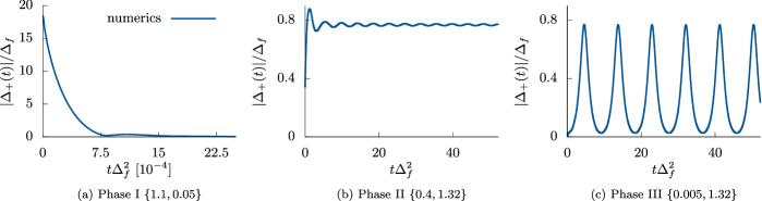
Figure 3: The magnitude of the $p+ip$ order parameter amplitude, $\lvert\Delta_{+}(t)\rvert$, for various interaction quenches, $G_{i}\to G_{f}$, in the $p+ip$ model Eq. (25). The behavior for the full $p$-wave Hamiltonian is the same when quenched exactly from the $p+ip$ ground state. The quench coordinates $\left\{\Delta_{i},\Delta_{f}\right\}$ correspond to the ground state value of the order parameter amplitude, $\Delta_{0,+}$, for the initial and final couplings $G_{i}$ and $G_{f}$, respectively. In phase I, the order parameter amplitude decays to zero due to dephasing, in phase II it exhibits power law damped oscillations and decays to a constant, and in phase III it exhibits persistent oscillations. The numerical simulations were performed on Eq. (22) for $N=50,000$ pseudospins, see Appendix A for details.

We begin by considering the dynamics of the two order parameters following a quench from the exact $p+ip$ ground state – Eq. (10) with $\Delta_{0,-}=0$. For such an initial state, the dynamics significantly simplify and it can formally be shown that they are equivalent to those generated from the pure $p+ip$ Hamiltonian [36]. To see this, we note that any time dependent $p+ip$ state can be written in the form

$$s_{\mathbf{k}}^{-}\equiv e^{-i\phi_{\mathbf{k}}}s_{k}^{-},\quad s_{\mathbf{k}}\equiv s_{k}^{z}.$$ (20)

Substituting Eq. (20) into Eq. (5), we find

$$\begin{split}\Delta_{-}&=-G\sum_{\mathbf{k}}ke^{-2i\phi_{\mathbf{k}}}s_{k}^{-}\\ &=-\frac{g}{2\pi^{2}}\int_{0}^{2\Lambda}\epsilon s^{-}(\epsilon)\mathrm{d}\epsilon\int_{0}^{\pi}e^{-2i\phi}\mathrm{d}\phi=0,\end{split}$$ (21)

where in the second line we have taken the continuum limit and performed the integral over $\phi$. The above equation shows that for any $p+ip$ initial state $\Delta_{-}$ remains zero throughout the entire evolution.

A similar substitution into the equations of motion Eq. (8) gives

$$\begin{split}\dot{s}_{k}^{-}=&-ik^{2}s_{k}^{-}+2iks_{k}^{z}\Delta_{+},\\ \dot{s}_{k}^{z}=&-ik\left(s_{k}^{+}\Delta_{+}-s_{k}^{-}\Delta_{+}^{*}\right).\end{split}$$ (22)

Eq. (22) is identical to the equations of motion that are generated by the $p+ip$ Hamiltonian. The $p+ip$ Hamiltonian is a truncated version of the full $p$-wave Hamiltonian Eq. (1) where by writing,

$$\mathbf{k}\cdot\mathbf{q}=\frac{1}{2}\left[(k^{x}-ik^{y})(q^{x}+iq^{y})+(k^{x}+ik^{y})(q^{x}-iq^{y})\right],$$ (23)

discarding the second term, keeping only $\mathbf{p}=0$ terms in the interaction as before, and rewriting the fermionic operators in terms of the Anderson pseudospins we arrive at

$$\hat{H}=\sum_{\mathbf{k}}^{\prime}k^{2}\hat{s}^{z}_{\mathbf{k}}-G\sum_{\mathbf{k},\mathbf{q}}^{\prime}(k^{x}-ik^{y})(q^{x}+iq^{y})\hat{s}_{\mathbf{k}}^{+}\hat{s}_{\mathbf{q}}^{-}.$$ (24)

The mean field Hamiltonian simplifies to

$$\hat{H}_{MF}^{p+ip}=\sum_{\mathbf{k}}^{\prime}k^{2}\hat{s}^{z}_{\mathbf{k}}+\sum_{\mathbf{k}}^{\prime}k\left(e^{-i\phi_{\mathbf{k}}}\Delta_{+}\hat{s}_{\mathbf{k}}^{+}+e^{+i\phi_{\mathbf{k}}}\Delta_{+}^{*}\hat{s}_{\mathbf{k}}^{-}\right).$$ (25)

The equations of motion generated by this Hamiltonian after applying Eq. (20) are Eq. (22). Note that we can alternatively start from a $p-ip$ ground state and follow a similar logic. The result is again Eq. (22), but with the replacement $\Delta_{+}\rightarrow\Delta_{-}$. The $p-ip$ Hamiltonian analogous to Eq. (24) would then correspond to discarding the first term in Eq. (23).

This simplification is crucial in understanding the $p+ip$ dynamics of the $p$-wave superfluid as the mean field $p+ip$ model was shown to be classically integrable using a Lax vector construction [36], which implies Lax pair representation of the equations of motion Eq. (22), see Ref. [67] for details. By studying the behavior of the isolated roots of the Lax vector norm, the quench phase diagram can be mapped out [68, 69, 36, 58]. We repeat this procedure in Appendix C for the parameters used in our numerical simulations. The resulting phase diagram contains three distinct dynamical phases characterized by the late time behavior of the order parameter amplitude $\Delta_{+}(t)$.

In phase I, the order parameter amplitude decays to zero due to dephasing, $\lvert\Delta_{+}(t)\rvert\rightarrow 0$. At late times, the spins precess with frequencies $k^{2}$ around the $z$-axis and the system is in a gapless superconducting state. This is different from the normal state which would have all spins aligned along the $z$-axis.

In phase II, $|\Delta_{+}(t)|$ exhibits damped oscillations and decays to a nonzero constant, $\lvert\Delta_{+}(t)\rvert\rightarrow\Delta_{\infty}>0$. The order parameter amplitude has a time dependent phase that winds with frequency $2\mu_{\infty}$, i.e.,

$$\Delta_{+}(t)=\Delta_{\infty}e^{-2i\mu_{\infty}t},$$ (26)

similar to its ground state behavior in Eq. (9). This suggests that that $\mu_{\infty}$ is an out of equilibrium chemical potential whose value is determined by the details of the quench. In the rotating frame, the pseudospins precess around an effective field

$$\mathbf{h}_{\mathbf{k}}=-(2k\cos\phi_{\bf k}\Delta_{\infty})\hat{\bf x}-(2k\sin\phi_{\bf k}\Delta_{\infty})\hat{\bf y}-(k^{2}-2\mu_{\infty})\hat{\bf z}.$$

The expression for the field is of the same form as in the ground state, see Eq. (17), and therefore,

$$W=\frac{1}{2}\left[1+\mathrm{sgn}(\mu_{\infty})\right].$$ (27)

This is similar to the ground state result, Eq. (18), but with the replacement $\mu\rightarrow\mu_{\infty}$. We conclude that the change in $W$ at $\mu_{\infty}=0$ marks the nonequilibrium extension of the quantum critical point. In Appendix D, we show that $\mu_{\infty}=0$ defines a straight vertical line $\Delta_{f}=\Delta_{\mathrm{QCP}}$ in the quench phase diagram [57] as shown in Fig. 1.

In phase III, the order parameter amplitude undergoes persistent oscillations that can be described in terms of elliptic functions. Additionally, it was shown in Ref. 37 that in multiple regions of this phase there are crossing edge states suggesting that the entire phase is Floquet topological. The order parameter dynamics for each of the phases are shown in Fig. 3 using a numerical simulation of Eq. (22). For details regarding the numerics see Appendix A.

It is somewhat surprising that the quench dynamics of the full $p$-wave Hamiltonian can be solved exactly for quenches from a pure $p+ip$ ground state given that this Hamiltonian is nonintegrable. To what extent the dynamics and topological structure survive infinitesimally small perturbations from this fine tuned initial state is studied in the following sections.

IV Full p-wave dynamics

Naturally, the system cannot be prepared in a $p+ip$ ground state, where $\Delta_{0,-}=0$, with absolute purity. Inevitably, there are fluctuations around this state that can come from a variety of sources. We will see below that pure $p+ip$ oscillatory dynamics are unstable towards exponential growth of the competing $p-ip$ order associated with $\Delta_{0,-}$. Therefore, the precise mechanism of the fluctuations is unimportant as long as they seed a nonzero initial $\Delta_{0,-}$. To understand the effect of such fluctuations we study quenches from an initial state described by Eq. (10) with $0<\Delta_{0,-}\ll\Delta_{0,+}$. We find that, in the limit $\Delta_{0,-}\to 0$, the phase diagram remains largely unaffected with the exception of phase III, wherein $\Delta_{-}(t)$ undergoes an unstable growth and the smooth oscillatory dynamics of $\Delta_{+}(t)$ are destroyed.

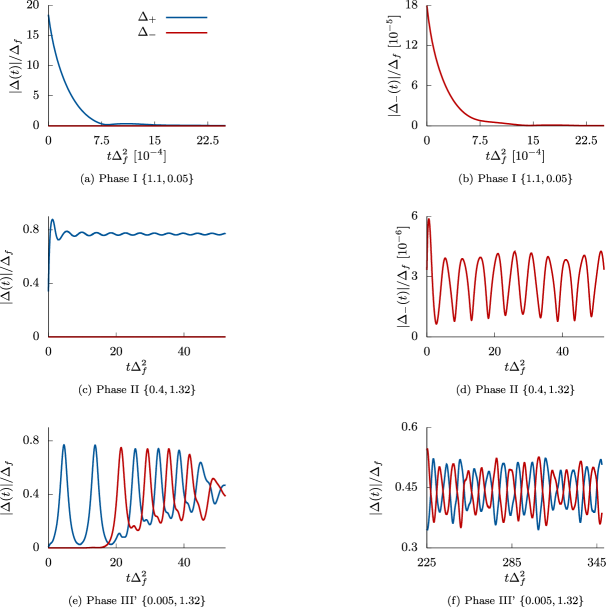
Figure 4: Dynamics of order parameter amplitudes $\lvert\Delta_{+}(t)\rvert$ and $\lvert\Delta_{-}(t)\rvert$ for a quenched $p$-wave superfluid starting from a slightly perturbed $p+ip$ ground state. In phase I, (a) and (b), both order parameter amplitudes decay to zero. In phase II, (c) and (d), $\Delta_{+}(t)$ has damped oscillations and decays to a nonzero constant while $\Delta_{-}(t)$ has small and smooth oscillations. In both of these phases, $\Delta_{-}(t)$ is bounded and the dynamics of $\Delta_{+}(t)$ are unchanged. In phase III’, (e) and (f), the $\Delta_{-}$ perturbation grows and destroys the persistent oscillations exhibited by the $p+ip$ model, see Fig. 3c. At late times, the irregular oscillations of both order parameter amplitudes are out of phase with each other. As in the previous figure, the numbers in the curly brackets are the ground state values of $\Delta_{0,+}$ for the initial and final couplings. The numerical simulations were performed on Eq. (8) for $N=200,025$ pseudospins with initial conditions Eq. (10) and $\Delta_{0,-}=10^{-5}\Delta_{0,+}$, see Appendix A for details.

IV.1 Stable phases I and II

For quenches whose coordinates lie within phases I or II of the $p+ip$ phase diagram, the dynamics of the full $p$-wave Hamiltonian closely mirror that of the truncated $p+ip$ model, as shown in Fig. 4. In phase I, we find that both $\Delta_{+}(t)$ and $\Delta_{-}(t)$ decay to zero in a similar fashion. As before, at late times the pseudospins precess around the the $z$-axis with frequencies $k^{2}$. In phase II, $\Delta_{+}(t)$ exhibits damped oscillations and decays to a constant. On the other hand, $\Delta_{-}(t)$ exhibits smooth oscillations that do not seem to decay. The perturbation to the initial state does not affect the dynamics significantly since at $t=0$ we have $\Delta_{-}(0)/\Delta_{+}(0)\ll 1$ and as $t\rightarrow\infty$ the size of $\Delta_{-}(t)$ remains bounded and is negligible as compared to $\Delta_{+}(t)$. The asymptotic state of the system is largely unaffected by the perturbation to the initial state and thus we expect the nonequilibrium topology of phases I and II to remain unchanged.

IV.2 Unstable phase III

From numerical simulations we find the persistent oscillations observed in phase III are not stable to the $\Delta_{-}$ perturbation. Unlike in phases I and II, the $p-ip$ order parameter amplitude exhibits unstable growth, and after some delay time, $\tau$, the persistent oscillations are destroyed and the system enters a regime of chaotic dynamics which we label as phase III’. Since quenches from $g_{i}=0$ to not too large $g_{f}$ belong to phase III’, we can understand the behavior in this phase by linearizing the equations of motion about the unpaired (free Fermi gas) ground state, which has $\Delta_{i}=0$ and $\mu_{i}=2\pi n$. In the continuum limit, the growth exponent $\gamma$ is defined through the self-consistency equation of the linearized problem

$$\frac{2\pi}{g_{f}}=\int_{0}^{2\Lambda}\mathrm{d}\epsilon\frac{\epsilon\,\mathrm{sgn}(\epsilon-2\mu_{i})}{\epsilon-\zeta}$$ (28)

where $\zeta=\omega+i\gamma$. We can rewrite $g_{f}$ in terms of $\Delta_{f}$ through Eq. (13) and perform the corresponding integrals on both sides of the equation. Discarding terms of order $O(\Lambda^{-1})$, we obtain

$$\zeta\log\left[\frac{-(2\mu_{i}-\zeta)^{2}}{2\Lambda\zeta}\right]=2\mu_{f}\log\left[\frac{\Delta_{f}^{2}+2\lvert\mu_{f}\rvert\Theta(-\mu_{f})}{2\Lambda}\right].$$ (29)

To simplify the analysis we may consider a quench to weak final pairing $\Delta_{f}\ll\Delta_{\mathrm{QCP}}$. In this case we can take $\mu_{i}\sim\mu_{f}\gg\Delta_{f}^{2}$ and look for solutions of the form $\zeta=2\mu_{i}+i\gamma$ for which we find $\gamma=\Delta_{f}\sqrt{2\mu_{i}}$. From numerical simulations we find the initial growth of $\Delta_{-}(t)$ to be suppressed by nonlinear effects and occurring at later times than predicted by the linear analysis.

We can also use Eq. (29) to determine the point separating nonequilibrium phases II and III’ along the $\Delta_{f}$ axis. As we cross from phase III’ to II, the imaginary part of $\zeta$ vanishes, removing the exponential growth of $\Delta_{-}(t)$. Setting $\gamma=0$, we see that the only possible solutions are for $\omega\leq 0$. Rewriting Eq. (29) in terms of $\omega$ we have

$$-\lvert\omega\rvert\log\left[\frac{(2\mu_{i}+\lvert\omega\rvert)^{2}}{2\Lambda\lvert\omega\rvert}\right]=2\mu_{f}\log\left[\frac{\Delta_{f}^{2}+2\lvert\mu_{f}\rvert\Theta(-\mu_{f})}{2\Lambda}\right].$$ (30)

In order to have real solutions for $\omega$, we must require that $\mu_{f}\leq 0$. This first happens when $\Delta_{f}=\Delta_{\mathrm{QCP}}$ where $\mu_{f}=0$ and, therefore, the quantum critical point defines the separation point, see Fig. 1.

Interestingly, this stability analysis also has important implications for the equilibrium physics of the $p$-wave superfluid. Indeed, we investigated here the stability of the unpaired ground state (normal state) with respect to the $p$-wave Hamiltonian Eq. (3) with coupling $G=G_{f}$ and found that this state is unstable in the BCS phase, when the ground state pairing amplitude is smaller then $\Delta_{\mathrm{QCP}}$, and stable in the BEC phase, when it exceeds $\Delta_{\mathrm{QCP}}$. Thus, the change in stability of the normal state state identifies the BCS-BEC quantum phase transition. We note also that our analysis of the free energy shows that even though the normal state is dynamically stable in the BEC state, it is not a local minimum of the free energy.

IV.3 Signatures of chaos

The late time dynamics in phase III’ appear to be chaotic in contrast to phase III of the $p+ip$ model. We believe this is because the full $p$-wave model, Eq. (3), is nonintegrable unlike its truncated $p+ip$ counterpart, Eq. (24). One piece of evidence of chaos is that the dynamics are sensitive to the initial conditions, as demonstrated in Fig. 5, where varying the magnitude of the $\Delta_{-}$ perturbation yields vastly different late time trajectories. This behavior makes it difficult to obtain reliable numerical results at late times since increasing the number of spins effectively modifies the initial conditions. However, the qualitative behavior, i.e., the appearance of irregular oscillations, is the same. Additionally, the Fourier spectrum of the time series changes from a discrete frequency in the classically integrable $p+ip$ case to a continuous spectrum in the full $p$-wave case as shown in Fig. 6.

IV.4 Phase III’ topology

At late times, the irregular oscillations of the two order parameters are out of phase with one another. The system dynamics are no longer periodic and the Floquet topological superfluid phase seen in Ref. [37] is therefore destroyed. Due to the chaotic nature of the dynamics there is no remnant of topological order in any known sense in the system.

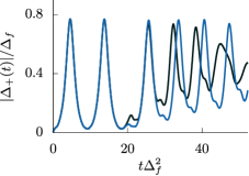
Figure 5: For a quench in phase III’, two trajectories whose initial conditions vary only slightly will rapidly diverge. The $\Delta_{-}$ perturbations are given by $\Delta_{0,-}=1\cdot 10^{-5}\Delta_{0,+}$ and $\Delta_{0,-}=2\cdot 10^{-5}\Delta_{0,+}$ for a quench with coordinates $\{\Delta_{i},\Delta_{f}\}=\{0.005,1.32\}$. Other parameters and conventions are the same as in the previous figure.

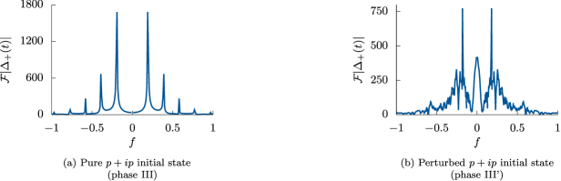
Figure 6: Fourier transform of the pairing amplitude $\lvert\Delta_{+}(t)\rvert$ for a quench from (a) pure $p+ip$ ground state and (b) perturbed $p+ip$ ground state in the full $p$-wave model. The perturbation and quench parameters are the same as in Fig. 5. Spectrum (a) shows a single independent frequency characteristic of the Floquet topological superfluid phase III of the truncated $p+ip$ model. The perturbation makes the spectrum continuous in (b) suggesting chaotic dynamics in phase III’, which replaces phase III in the full $p$-wave model, and indicating the destruction of the Floquet topological order.

IV.5 Determination of the phase boundaries

Although the full $p$-wave Hamiltonian is nonintegrable, it is possible to determine the phase boundaries analytically. We have seen that the dynamics of $\Delta_{+}(t)$ in phases I and II are nearly identical to those of the $p+ip$ model. We can therefore expect this phase boundary to remain unchanged. In phase III’, we have seen that there is an instability of $\Delta_{-}(t)$ that leads to chaotic dynamics of both the orders at late times. However, this instability is confined to the phase III region of the $p+ip$ model and again there is no choice but for the phase boundary to remain unchanged between phases II and III’. The exact phase boundaries for the full $p$-wave model can then be determined by performing the same analysis of the Lax roots outlined in Ref. 36. This is done in Appendix C and the result is used to generate the phase diagram shown in Fig. 1. These phase boundaries are in agreement with direct numerical simulations of the dynamics. We also expect the $\mu_{\infty}=0$ line to remain unchanged since it lies entirely within the stable phase II.

There are differences between shapes of the various lines in our phase diagram as compared to that of Ref. 36 due to the cutoff prescription of Ref. 36, which incorporates the chemical potential, i.e., replaces our $\Lambda$ with $\Lambda+\mu$ with $\mu$ being the equilibrium chemical potential. Because $\mu$ depends on the coupling constant, this cutoff changes as a result of a quench. The cutoff represents an energy scale governed by physics at higher energies, such as, e.g., the Debye energy in phonon mediated superconductors. It is more natural to keep this energy scale fixed and unaffected by the quench. We therefore use a fixed cutoff throughout the quench phase diagram, which also results in simpler and more intuitive line shapes. In particular, our phase III’ boundary terminates at $\Delta_{\mathrm{QCP}}$ along the $\Delta_{f}$ axis and our $\mu_{\infty}=0$ line is a straight vertical line defined by the equation $\Delta_{f}=\Delta_{\mathrm{QCP}}$.

V Stability of the p-wave superfluid with respect to time reversal symmetry breaking 

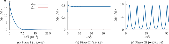
Figure 7: The time reversal symmetry of the $p$-wave interaction is broken by making one of the interaction channels stronger, here we have used $G_{+}>G_{-}$. The figures shown are representative of the two order parameter amplitudes in all three phases for a quench from a slightly perturbed $p+ip$ ground state. The $\Delta_{-}$ perturbation is irrelevant to the late time dynamics of $\Delta_{+}(t)$ as it rapidly vanishes in all three phases. The resulting dynamics of $\Delta_{+}(t)$ closely resemble the pure $p+ip$ quench dynamics. Notations and unspecified parameters are the same as in Fig. 4.

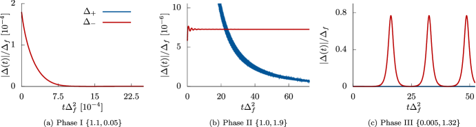
Figure 8: Same as Fig. 7 but with $G_{+}<G_{-}$. Even though the $\Delta_{-}$ perturbation starts at $10^{-5}\Delta_{0,+}$, it is the one whose dynamics survive out to late times. The $p+ip$ order parameter amplitude vanishes in all three phases and the dynamics of $\Delta_{-}(t)$ closely resemble the pure $p-ip$ quench dynamics, though for a different set of quench coordinates. Note, in (a), $\Delta_{+}(t)$ vanishes slower than $\Delta_{-}(t)$ due to the relative sizes of $G_{+}$ and $G_{-}$ and so it does not show up with the scales used in the figure.

In the previous section, we have seen that the phase III dynamics are unstable to a perturbation of the pure $p+ip$ initial state. To understand the nature of this instability we study a variation of the Hamiltonian in Eq. (3) which explicitly breaks time reversal symmetry due to an asymmetry in the coupling. To each interaction channel we associate a distinct coupling constant, $G_{+}\neq G_{-}$,

$$\begin{split}\hat{H}^{\mathrm{asym}}=\sum_{\mathbf{k}}^{\prime}k^{2}\hat{s}^{z}_{\mathbf{k}}-G_{+}\sum_{\mathbf{k},\mathbf{q}}^{\prime}(k^{x}-ik^{y})(q^{x}+iq^{y})\hat{s}_{\mathbf{k}}^{+}\hat{s}_{\mathbf{q}}^{-}\\ -G_{-}\sum_{\mathbf{k},\mathbf{q}}^{\prime}(k^{x}+ik^{y})(q^{x}-iq^{y})\hat{s}_{\mathbf{k}}^{+}\hat{s}_{\mathbf{q}}^{-}\end{split}$$ (31)

and define new order parameter amplitudes

$$\Delta_{\pm}\equiv-G_{\pm}\sum_{\mathbf{k}}ke^{\pm i\phi_{\mathbf{k}}}\langle s_{\mathbf{k}}^{-}\rangle.$$ (32)

For $G_{+}=G_{-}$ this Hamiltonian turns into the full $p$-wave Hamiltonian Eq. (3) we studied above, see Eq. (23).

We consider quenches from a perturbed $p+ip$ initial state for the two cases where one channel dominates over the other employing the same approach to dynamics as before. For $G_{+}>G_{-}$, the dominant channel corresponds to the $p+ip$ channel. Using numerical simulations we find that for any quench, the $p-ip$ order parameter, $\Delta_{-}(t)$, quickly vanishes, as shown in Fig. 7. This result is to be expected as the $p-ip$ order is suppressed in both the initial state as well as by the equations of motion themselves.

For $G_{+}<G_{-}$, the dominant channel corresponds to the $p-ip$ channel and it is not immediately clear which channel the dynamics should favor. On one hand, the initial state favors the $p+ip$ channel while the $p-ip$ channel only acts as a perturbation, on the other hand, the equations of motion suppress the $p+ip$ channel and favor the $p-ip$ channel. We find that, in this case, the $p+ip$ order parameter is the one to rapidly decay to zero while the $p-ip$ order parameter survives to exhibit the late time dynamics (in phase I both order parameters decay to zero). This behavior is shown in Fig. 8, where even though $\Delta_{-}(0)/\Delta_{+}(0)\ll 1$, the $p-ip$ order parameter amplitude is the one with nonvanishing dynamics in phases II and III. These late time dynamics resemble the three phases of the pure $p\pm ip$ quench dynamics but with a renormalized set of quench coordinates. It is an interesting question as to whether the phase boundaries of the asymetric model, particularly for $G_{+}<G_{-}$, remain the same as in the chiral model or are deformed in some way.

We see that the stronger channel always wins at late times regardless of the initial state. This means that the time reversal invariant $p$-wave Hamiltonian is an unstable fixed point with regards to the $p\pm ip$ phase diagram. Only at the special point $G_{+}=G_{-}$ protected by time reversal symmetry does the chaotic phase III’ regime emerge, see Fig. 2.

VI Conclusion

In this work we have studied the quench dynamics of a $p$-wave BCS superfluid with two competing order parameters, $\Delta_{\pm}(t)$. We have shown that when the system is prepared near its $p+ip$ ground state and the interaction strength is quenched, the late time dynamics can be characterized into three distinct phases: in phase I both order parameters decay to zero, in phase II $\Delta_{+}(t)$ decays to a nonzero constant and $\Delta_{-}(t)$ oscillates near zero, and in phase III’ the two order parameters are nonzero and undergo chaotic dynamics, see Fig. 4. Remarkably, even though this model is nonintegrable, we are able to map out the exact phase boundaries in parameter space as shown in Fig. 1. Additionally, we study the role that time reversal symmetry plays in determining the late time dynamics. We consider a Hamiltonian that has an asymmetry in the coupling strength and prefers one of the order parameters over the other, i.e., $G_{+}\neq G_{-}$ in Eq. (31). We find that the late time dynamics of the weaker channel order parameter vanish and only the stronger channel survives. This causes the chaotic dynamics of phase III’ to disappear and the topological phase III of the chiral $p$-wave model studied in Ref. [36] to emerge. The fact that the stronger channel always wins suggests that it may be possible to experimentally realize a quench induced Floquet topological superfluid without any fine tuning of the initial state provided that time reversal symmetry can be broken in the interaction channels.

Although our analysis has only been performed for the $p$-wave BCS superfluid, we expect a similar chaotic phase to emerge in far from equilibrium dynamics of other models where there are competing order parameters related by a symmetry, for example, in a Fermi gas with more than two species of fermions with pairwise attraction between them [70, 71, 72, 73].

Appendix A Details of numerical simulations

The numerical simulations were done using the parameters listed in Table 1 and Table 2. For the full $p$-wave simulations, we use a radial momentum space grid so that $\epsilon=k^{2}$ are uniformly spaced for $\epsilon\in\left[0,2\Lambda\right]$ and along the angular direction $\theta$ is uniformly spaced in the upper half plane for $\theta\in\left[0,\pi\right]$. For the chiral dynamics, the problem reduces to one dimension and we can neglect the $\theta$ dependence. The number of spins used in the numerical simulations is chosen such that the results are converged at the times of interest. We find that to obtain converging results at late times, it is important to have a large number of points along the radial direction, $N_{\epsilon}$, whereas the results are not as sensitive to the number of points along the angular direction, $N_{\theta}$. Since we have few $N_{\epsilon}$ points in the full $p$-wave model, we use the composite Simpson’s rule to have a more accurate estimate of the integrals in the problem while for the chiral model we simply use the trapezoidal rule. Obtaining convergent results becomes difficult for quenches in phase III’ where the dynamics are chaotic. In order to reach later times we must increase $N_{\epsilon}$, but changing the number of points effectively changes the initial conditions. The results, however, are qualitatively the same, i.e., the Floquet phase is destroyed and irregular oscillations appear.

Quantity	Symbol	Value
Number of $\epsilon$ points	$N_{\epsilon}$	8001
Number of $\theta$ points	$N_{\theta}$	25
Density	$n$	0.825
Fermi Energy	$\epsilon_{F}$	$2\pi n$
High energy cutoff	$\Lambda$	$50\epsilon_{F}$
Quantum critical point	$\Delta_{\mathrm{QCP}}$	$\approx 1.536$
Ground state order parameter amplitude	$\Delta_{0,+}$	See figures for details
$\Delta_{-}$ perturbation	$\Delta_{0,-}$	$10^{-5}\Delta_{0,+}$

Table 1: Parameters used to simulate the full $p$-wave dynamics described by Eq. (8)

Quantity	Symbol	Value
Number of $\epsilon$ points	$N_{\epsilon}$	50000
Density	$n$	0.825
Fermi Energy	$\epsilon_{F}$	$2\pi n$
High energy cutoff	$\Lambda$	$50\epsilon_{F}$
Quantum critical point	$\Delta_{\mathrm{QCP}}$	$\approx 1.536$
Ground state order parameter amplitude	$\Delta_{0,+}$	See figures for details

Table 2: Parameters used to simulate the $p+ip$ dynamics described by Eq. (22)

Appendix B BCS equations

The integral on the right hand side of Eq. (14) for the particle density can be evaluated exactly

$$n=\frac{1}{8\pi}\left(2\Lambda+\lvert 2\mu\rvert-\sqrt{(2\Lambda-2\mu)^{2}+8\Delta_{+}^{2}\Lambda}+2\Delta_{+}^{2}\ln\left[\frac{2\Lambda-2\mu+2\Delta_{+}^{2}+\sqrt{(2\Lambda-2\mu)^{2}+8\Delta_{+}^{2}\Lambda}}{2\Delta_{+}^{2}+\lvert 2\mu\rvert-2\mu}\right]\right).$$ (33)

Expanding the square root in $1/\Lambda$ and neglecting terms of order $\Lambda^{-1}$ and smaller leads to

$$4\pi n=2\mu\Theta(\mu)-\Delta^{2}_{+}+\Delta_{+}^{2}\ln\left[\frac{2\Lambda}{\Delta_{+}^{2}+2\lvert\mu\rvert\Theta(-\mu)}\right],$$ (34)

Similarly, Eq. (13) becomes

$$\frac{2\pi}{g}=2\Lambda-8\pi n+2\mu\ln\left[\frac{2\Lambda}{\Delta_{+}^{2}+2\lvert\mu\rvert\Theta(-\mu)}\right].$$ (35)

We use these results in Appendix C to derive the phase boundaries.

Appendix C Lax roots and quench phase diagram

In the $p+ip$ model, the components of the Lax vector are given by [36]

$$L^{\pm}(u)=\sum_{i=1}^{N}\frac{\sqrt{\epsilon_{i}}s_{i}^{\pm}}{\epsilon_{i}-u},\quad L^{z}(u)=\sum_{i=1}^{N}\frac{\epsilon_{i}s_{i}^{z}}{\epsilon_{i}-u}+\frac{1}{2G_{f}}$$ (36)

and one can define a Lax vector norm

$$L_{2}(u)=uL^{+}(u)L^{-}(u)+[L^{z}(u)]^{2},$$ (37)

that is conserved under the dynamics. The Lax vector norm is a polynomial of degree $2N$ whose isolated roots encode information about the late time dynamics [68, 69, 36, 58]. Specifically, phase I occurs when $L_{2}(u)$ has no isolated roots (the remaining roots form a continuum on the positive real axis). Phase II corresponds to a single pair and phase III to two pairs of isolated roots. To find the roots, we can evaluate $L_{2}(u)$ in the initial state which has the configuration described by Eq. (10) with $\Delta_{0,-}=0$ and $\Delta_{0,+}\equiv\Delta_{i}$, i.e.,

$$\begin{split}s_{i}^{-}=-\frac{\sqrt{\epsilon_{i}}\Delta_{i}}{E(\epsilon_{i})}&,\qquad s_{i}^{z}=-\frac{(\epsilon_{i}-2\mu_{i})}{2E(\epsilon_{i})},\\ E(\epsilon)=&\sqrt{(\epsilon-2\mu_{i})^{2}+4\epsilon\lvert\Delta_{i}\rvert^{2}}.\end{split}$$ (38)

Substituting into the above equations, the Lax vector norm becomes

$$L_{2}(u)=u\lvert\Delta_{i}\rvert^{2}\left[\sum_{i}\frac{\epsilon_{i}}{(\epsilon_{i}-u)E(\epsilon_{i})}\right]^{2}+\left[-\sum_{i}\frac{\epsilon_{i}(\epsilon_{i}-2\mu_{i})}{2(\epsilon_{i}-u)E(\epsilon_{i})}+\frac{1}{2G_{f}}\right]^{2}.$$ (39)

This equation can be simplified to

$$L_{2}(u)=u\lvert\Delta_{i}\rvert^{2}\left[F(u)\right]^{2}+\left[-\frac{(u-2\mu_{i})}{2}F(u)+\frac{\tilde{\beta}}{2}\right]^{2}$$ (40)

by defining

$$\tilde{\beta}\equiv\frac{1}{G_{f}}-\frac{1}{G_{i}},\quad F(u)\equiv\sum_{i}\frac{\epsilon_{i}}{(\epsilon_{i}-u)E(\epsilon_{i})}.$$ (41)

The roots of the Lax vector norm are found by solving the quadratic equation for $F(u)$

$$L_{2}(u)=E(u)^{2}F(u)^{2}-2(u-2\mu_{i})\tilde{\beta}F(u)+\tilde{\beta}^{2}=0,$$ (42)

with solutions given by

$$F(u)=\frac{(u-2\mu_{i})\tilde{\beta}\pm 2i\lvert\Delta_{i}\rvert\lvert\tilde{\beta}\rvert\sqrt{u}}{E(u)^{2}}.$$ (43)

Isolated roots are located away from the positive real axis. Eq. (43) for such roots in the continuum limit becomes

$$\int_{0}^{2\Lambda}\frac{\epsilon\mathrm{d}\epsilon}{(\epsilon-u)E(\epsilon)}=\frac{(u-2\mu_{i})\beta\pm 2i\lvert\Delta_{i}\rvert\lvert\beta\rvert\sqrt{u}}{E(u)^{2}},$$ (44)

with

$$\beta=2\pi\left(\frac{1}{g_{f}}-\frac{1}{g_{i}}\right).$$ (45)

To determine the phase boundaries we look for a pair of complex roots that just separate from (or collapse to) the real axis. To do this, we replace $u\rightarrow u\pm i\delta$ in Eq. (44), with $\delta$ infinitesimally small. Through a change of variables $x=\epsilon-u$ we may write

$$\int_{-u}^{2\Lambda-u}\frac{(x+u)\mathrm{d}x}{(x\mp i\delta)E(x+u)}=\mathcal{P}\int\frac{(x+u)\mathrm{d}x}{xE(x+u)}\pm i\pi\frac{u}{E(u)}$$ (46)

where $\mathcal{P}$ denotes the principal value.

Comparing the imaginary parts of the right hand sides of Eq. (46) and Eq. (44) we find

$$\lvert\beta\rvert=\frac{\pi\sqrt{u}E(u)}{2\lvert\Delta_{i}\rvert},$$ (47)

and comparing the real parts we find

$$\ln\left[\frac{2\Lambda}{\Delta_{i}^{2}+2\lvert\mu_{i}\rvert\Theta(-\mu_{i})}\right]+\frac{u}{E(u)}\ln\left[-\frac{2\left[u(\Delta_{i}^{2}-\mu_{i})+2\mu_{i}^{2}+\lvert\mu_{i}\rvert E(u)\right]}{u\left[u+2\Delta_{i}^{2}-2\mu_{i}+E(u)\right]}\right]=\mathrm{sgn}(\beta)\frac{\pi\sqrt{u}(u-2\mu_{i})}{2\lvert\Delta_{i}\rvert E(u)},$$ (48)

where we have neglected terms of order $O(\Lambda^{-1})$.

Equations (45), (47), and (48) form a system of equations that paramaterize the phase boundaries. By choosing a value for $\Delta_{i}$ and $\mathrm{sgn}(\beta)$, Eq. (48) can be solved for $u$ which can be substituted into Eq. (47) to determine $\beta$. Then, with the help of Eq. (45), $\Delta_{i}$ can be written as a function of $\Delta_{f}$ to map out the phase boundaries. This is the approach we used to obtain the phase boundaries shown in Fig. 1.

Appendix D Nonequilibrium extension of the quantum critical point

The nonequilibrium extension of the quantum critical point corresponds to the curve in phase II which has $\mu_{\infty}=0$. This line separates the two topological regions with field winding number, $W$, either zero or one. To determine the curve we look for the vanishing of an isolated root i.e., $u=0$ [36]. Substituting $u=0$ into Eq. (44) we have

$$\int_{0}^{2\Lambda}\frac{\epsilon\mathrm{d}\epsilon}{\epsilon E(\epsilon)}=-\frac{\beta}{2\mu_{i}}.$$ (49)

Evaluating the integral we find

$$\beta=-2\mu_{i}\log\left[\frac{2\Lambda}{\Delta_{i}^{2}+2\lvert\mu_{i}\rvert\Theta(-\mu_{i})}\right].$$ (50)

As before, we can use Eq. (45) to write $\Delta_{i}$ as a function of $\Delta_{f}$. The result simplifies to

$$\mu_{f}\log\left[\frac{2\Lambda}{\Delta_{f}^{2}+2\lvert\mu_{f}\rvert\Theta(-\mu_{f})}\right]=0$$ (51)

which can only be solved when $\mu_{f}=0$. In other words, for any $\Delta_{i}$ the value of $\Delta_{f}$ for which $\mu_{\infty}=0$ is given by $\Delta_{f}=\Delta_{\mathrm{QCP}}$, see the dashed line in the phase diagram in Fig. 1. This line remains unchanged in the full $p$-wave phase diagram since it lies entirely within the stable phase II.

References

- Kinoshita et al. [2006] T. Kinoshita, T. Wenger, and D. S. Weiss, A quantum Newton’s cradle, Nature 440, 900 (2006).
- Lignier et al. [2007] H. Lignier, C. Sias, D. Ciampini, Y. Singh, A. Zenesini, O. Morsch, and E. Arimondo, Dynamical control of matter-wave tunneling in periodic potentials, Phys. Rev. Lett. 99, 220403 (2007).
- Smale et al. [2019] S. Smale, P. He, B. A. Olsen, K. G. Jackson, H. Sharum, S. Trotzky, J. Marino, A. M. Rey, and J. H. Thywissen, Observation of a transition between dynamical phases in a quantum degenerate Fermi gas, Sci. Adv. 5, eaax1568 (2019).
- Tang et al. [2018] Y. Tang, W. Kao, K.-Y. Li, S. Seo, K. Mallayya, M. Rigol, S. Gopalakrishnan, and B. L. Lev, Thermalization near integrability in a dipolar quantum Newton’s cradle, Phys. Rev. X 8, 021030 (2018).
- Langen et al. [2015] T. Langen, S. Erne, R. Geiger, B. Rauer, T. Schweigler, M. Kuhnert, W. Rohringer, I. E. Mazets, T. Gasenzer, and J. Schmiedmayer, Experimental observation of a generalized Gibbs ensemble, Science 348, 207 (2015).
- Hofferberth et al. [2007] S. Hofferberth, I. Lesanovsky, B. Fischer, T. Schumm, and J. Schmiedmayer, Non-equilibrium coherence dynamics in one-dimensional Bose gases, Nature 449, 324 (2007).
- Weiler et al. [2008] C. N. Weiler, T. W. Neely, D. R. Scherer, A. S. Bradley, M. J. Davis, and B. P. Anderson, Spontaneous vortices in the formation of Bose–Einstein condensates, Nature 455, 948 (2008).
- Widera et al. [2008] A. Widera, S. Trotzky, P. Cheinet, S. Fölling, F. Gerbier, I. Bloch, V. Gritsev, M. D. Lukin, and E. Demler, Quantum spin dynamics of mode-squeezed Luttinger liquids in two-component atomic gases, Phys. Rev. Lett. 100, 140401 (2008).
- Gring et al. [2012] M. Gring, M. Kuhnert, T. Langen, T. Kitagawa, B. Rauer, M. Schreitl, I. Mazets, D. A. Smith, E. Demler, and J. Schmiedmayer, Relaxation and prethermalization in an isolated quantum system, Science 337, 1318 (2012).
- Bloch et al. [2008] I. Bloch, J. Dalibard, and W. Zwerger, Many-body physics with ultracold gases, Rev. Mod. Phys. 80, 885 (2008).
- Regal et al. [2004] C. A. Regal, M. Greiner, and D. S. Jin, Observation of resonance condensation of fermionic atom pairs, Phys. Rev. Lett. 92, 040403 (2004).
- Bloch et al. [2012] I. Bloch, J. Dalibard, and S. Nascimbene, Quantum simulations with ultracold quantum gases, Nat. Phys. 8, 267 (2012).
- Zwierlein et al. [2005] M. W. Zwierlein, J. R. Abo-Shaeer, A. Schirotzek, C. H. Schunck, and W. Ketterle, Vortices and superfluidity in a strongly interacting Fermi gas, Nature 435, 1047 (2005).
- Zwierlein et al. [2004] M. W. Zwierlein, C. A. Stan, C. H. Schunck, S. M. F. Raupach, A. J. Kerman, and W. Ketterle, Condensation of pairs of fermionic atoms near a Feshbach resonance, Phys. Rev. Lett. 92, 120403 (2004).
- Arute et al. [2020] F. Arute, K. Arya, R. Babbush, D. Bacon, J. C. Bardin, R. Barends, S. Boixo, M. Broughton, B. B. Buckley, D. A. Buell, et al., Hartree-Fock on a superconducting qubit quantum computer, Science 369, 1084 (2020).
- Gong et al. [2021] M. Gong, S. Wang, C. Zha, M.-C. Chen, H.-L. Huang, Y. Wu, Q. Zhu, Y. Zhao, S. Li, S. Guo, et al., Quantum walks on a programmable two-dimensional 62-qubit superconducting processor, Science 372, 948 (2021).
- Satzinger et al. [2021] K. Satzinger, Y. Liu, A. Smith, C. Knapp, M. Newman, C. Jones, Z. Chen, C. Quintana, X. Mi, A. Dunsworth, et al., Realizing topologically ordered states on a quantum processor (2021), arXiv:2104.01180 [quant-ph] .
- Cong et al. [2021] I. Cong, S.-T. Wang, H. Levine, A. Keesling, and M. D. Lukin, Hardware-efficient, fault-tolerant quantum computation with Rydberg atoms (2021), arXiv:2105.13501 [quant-ph] .
- Monroe et al. [2021] C. Monroe, W. C. Campbell, L.-M. Duan, Z.-X. Gong, A. V. Gorshkov, P. W. Hess, R. Islam, K. Kim, N. M. Linke, G. Pagano, et al., Programmable quantum simulations of spin systems with trapped ions, Rev. Mod. Phys. 93, 025001 (2021).
- Fausti et al. [2011] D. Fausti, R. Tobey, N. Dean, S. Kaiser, A. Dienst, M. C. Hoffmann, S. Pyon, T. Takayama, H. Takagi, and A. Cavalleri, Light-induced superconductivity in a stripe-ordered cuprate, Science 331, 189 (2011).
- Giannetti et al. [2016] C. Giannetti, M. Capone, D. Fausti, M. Fabrizio, F. Parmigiani, and D. Mihailovic, Ultrafast optical spectroscopy of strongly correlated materials and high-temperature superconductors: a non-equilibrium approach, Adv. Phys. 65, 58 (2016).
- Kampfrath et al. [2013] T. Kampfrath, K. Tanaka, and K. A. Nelson, Resonant and nonresonant control over matter and light by intense terahertz transients, Nat. Photonics 7, 680 (2013).
- Matsunaga et al. [2014] R. Matsunaga, N. Tsuji, H. Fujita, A. Sugioka, K. Makise, Y. Uzawa, H. Terai, Z. Wang, H. Aoki, and R. Shimano, Light-induced collective pseudospin precession resonating with Higgs mode in a superconductor, Science 345, 1145 (2014).
- Shimano and Tsuji [2020] R. Shimano and N. Tsuji, Higgs mode in superconductors, Annu. Rev. Condens. Matter Phys. 11, 103 (2020).
- Matsunaga et al. [2013] R. Matsunaga, Y. I. Hamada, K. Makise, Y. Uzawa, H. Terai, Z. Wang, and R. Shimano, Higgs amplitude mode in the BCS superconductors induced by terahertz pulse excitation, Phys. Rev. Lett. 111, 057002 (2013).
- Demsar [2020] J. Demsar, Non-equilibrium phenomena in superconductors probed by femtosecond time-domain spectroscopy, J. Low Temp. Phys. 201, 676 (2020).
- Schollwöck [2005] U. Schollwöck, The density-matrix renormalization group, Rev. Mod. Phys. 77, 259 (2005).
- Rigol et al. [2007] M. Rigol, V. Dunjko, V. Yurovsky, and M. Olshanii, Relaxation in a completely integrable many-body quantum system: an ab initio study of the dynamics of the highly excited states of 1D lattice hard-core bosons, Phys. Rev. Lett. 98, 050405 (2007).
- Kamenev and Levchenko [2010] A. Kamenev and A. Levchenko, Keldysh technique and non-linear -model: basic principles and applications, Adv. Phys. (2010).
- Polkovnikov [2010] A. Polkovnikov, Phase space representation of quantum dynamics, Ann. Phys. 325, 1790 (2010).
- Essler and Fagotti [2016] F. H. Essler and M. Fagotti, Quench dynamics and relaxation in isolated integrable quantum spin chains, J. Stat. Mech. Theory Exp. 2016, 064002 (2016).
- Calabrese and Cardy [2016] P. Calabrese and J. Cardy, Quantum quenches in 1+1 dimensional conformal field theories, J. Stat. Mech. Theory Exp. 2016, 064003 (2016).
- Calabrese and Cardy [2006] P. Calabrese and J. Cardy, Time dependence of correlation functions following a quantum quench, Phys. Rev. Lett. 96, 136801 (2006).
- Vasseur and Moore [2016] R. Vasseur and J. E. Moore, Nonequilibrium quantum dynamics and transport: from integrability to many-body localization, J. Stat. Mech. Theory Exp. 2016, 064010 (2016).
- Eisert et al. [2015] J. Eisert, M. Friesdorf, and C. Gogolin, Quantum many-body systems out of equilibrium, Nat. Phys. 11, 124 (2015).
- Foster et al. [2013] M. S. Foster, M. Dzero, V. Gurarie, and E. A. Yuzbashyan, Quantum quench in a p+ip superfluid: Winding numbers and topological states far from equilibrium, Phys. Rev. B 88, 104511 (2013).
- Foster et al. [2014] M. S. Foster, V. Gurarie, M. Dzero, and E. A. Yuzbashyan, Quench-induced Floquet topological p-wave superfluids, Phys. Rev. Lett. 113, 076403 (2014).
- D’Alessio and Rigol [2015] L. D’Alessio and M. Rigol, Dynamical preparation of Floquet Chern insulators, Nat. Commun. 6, 1 (2015).
- Moessner and Sondhi [2017] R. Moessner and S. L. Sondhi, Equilibration and order in quantum Floquet matter, Nat. Phys. 13, 424428 (2017).
- Yang et al. [2018] C. Yang, L. Li, and S. Chen, Dynamical topological invariant after a quantum quench, Phys. Rev. B 97, 060304(R) (2018).
- Gong and Ueda [2018] Z. Gong and M. Ueda, Topological entanglement-spectrum crossing in quench dynamics, Phys. Rev. Lett. 121, 250601 (2018).
- Sun et al. [2018] W. Sun, C.-R. Yi, B.-Z. Wang, W.-W. Zhang, B. C. Sanders, X.-T. Xu, Z.-Y. Wang, J. Schmiedmayer, Y. Deng, X.-J. Liu, and et al., Uncover topology by quantum quench dynamics, Phys. Rev. Lett. 121, 250403 (2018).
- McGinley and Cooper [2019] M. McGinley and N. R. Cooper, Interacting symmetry-protected topological phases out of equilibrium, Phys. Rev. Res. 1, 033204 (2019).
- Tonielli et al. [2020] F. Tonielli, J. C. Budich, A. Altland, and S. Diehl, Topological field theory far from equilibrium, Phys. Rev. Lett. 124, 240404 (2020).
- Tarnowski et al. [2019] M. Tarnowski, F. N. Ünal, N. Fläschner, B. S. Rem, A. Eckardt, K. Sengstock, and C. Weitenberg, Measuring topology from dynamics by obtaining the Chern number from a linking number, Nat. Commun. 10, 1 (2019).
- Kitagawa et al. [2010] T. Kitagawa, E. Berg, M. Rudner, and E. Demler, Topological characterization of periodically driven quantum systems, Phys. Rev. B 82, 235114 (2010).
- Else and Nayak [2016] D. V. Else and C. Nayak, Classification of topological phases in periodically driven interacting systems, Phys. Rev. B 93, 201103(R) (2016).
- Potter et al. [2016] A. C. Potter, T. Morimoto, and A. Vishwanath, Classification of interacting topological Floquet phases in one dimension, Phys. Rev. X 6, 041001 (2016).
- Roy and Harper [2017] R. Roy and F. Harper, Periodic table for Floquet topological insulators, Phys. Rev. B 96, 155118 (2017).
- Wang et al. [2017] C. Wang, P. Zhang, X. Chen, J. Yu, and H. Zhai, Scheme to measure the topological number of a Chern insulator from quench dynamics, Phys. Rev. Lett. 118, 185701 (2017).
- Read and Green [2000] N. Read and D. Green, Paired states of fermions in two dimensions with breaking of parity and time-reversal symmetries and the fractional quantum Hall effect, Phys. Rev. B 61, 10267 (2000).
- Volovik [2003] G. E. Volovik, The universe in a helium droplet, Vol. 117 (Oxford University Press on Demand, 2003).
- Gurarie and Radzihovsky [2007] V. Gurarie and L. Radzihovsky, Resonantly paired fermionic superfluids, Ann. Phys. 322, 2 (2007).
- Chin et al. [2010] C. Chin, R. Grimm, P. Julienne, and E. Tiesinga, Feshbach resonances in ultracold gases, Rev. Mod. Phys. 82, 1225 (2010).
- Yuzbashyan and Tsyplyatyev [2009] E. A. Yuzbashyan and O. Tsyplyatyev, Dynamics of emergent Cooper pairing at finite temperatures, Phys. Rev. B 79, 132504 (2009).
- Dzero et al. [2009] M. Dzero, E. A. Yuzbashyan, and B. L. Altshuler, Cooper pair turbulence in atomic fermi gases, Europhys. Lett. 85, 20004 (2009).
- Note [1] There are differences in the shapes of phase boundaries and line between our Fig. 1 and Ref. \rev@citealpFoster_2013 due to different cutoff conventions, see the end of Sec. IV.5.
- Yuzbashyan et al. [2015] E. A. Yuzbashyan, M. Dzero, V. Gurarie, and M. S. Foster, Quantum quench phase diagrams of an s-wave BCS-BEC condensate, Phys. Rev. A 91, 033628 (2015).
- Anderson [1958] P. W. Anderson, Random-phase approximation in the theory of superconductivity, Phys. Rev. 112, 1900 (1958).
- Richardson [1977] R. W. Richardson, Pairing in the limit of a large number of particles, J. Math. Phys. 18, 1802 (1977).
- Roman et al. [2002] J. Roman, G. Sierra, and J. Dukelsky, Large N limit of the exactly solvable BCS model: Analytics versus numerics, Nucl. Phys. B 634, 483 (2002).
- Yuzbashyan et al. [2005] E. A. Yuzbashyan, A. A. Baytin, and B. L. Altshuler, Finite-size corrections for the pairing Hamiltonian, Phys. Rev. B 71, 094505 (2005).
- Faribault et al. [2009] A. Faribault, P. Calabrese, and J.-S. Caux, Quantum quenches from integrability: the fermionic pairing model, J. Stat. Mech. Theory Exp. , P03018 (2009).
- [64] A. Wu, A. Zabalo, J. H. Pixley, and E. A. Yuzbashyan, to appear.
- Homrighausen and Kehrein [2019] I. Homrighausen and S. Kehrein, Out of equilibrium mean field dynamics in the transverse field ising model (2019), arXiv:1908.02596 [cond-mat] .
- Alicea [2012] J. Alicea, New directions in the pursuit of majorana fermions in solid state systems, Rep. Prog. Phys. 75, 076501 (2012).
- Rylands et al. [2021] C. Rylands, E. A. Yuzbashyan, V. Gurarie, A. Zabalo, and V. Galitski, Loschmidt echo of far-from-equilibrium fermionic superfluids, Ann. Phys. , 168554 (2021).
- Yuzbashyan et al. [2006] E. A. Yuzbashyan, O. Tsyplyatyev, and B. L. Altshuler, Relaxation and persistent oscillations of the order parameter in fermionic condensates, Phys. Rev. Lett. 96, 097005 (2006).
- Yuzbashyan and Dzero [2006] E. A. Yuzbashyan and M. Dzero, Dynamical vanishing of the order parameter in a fermionic condensate, Phys. Rev. Lett. 96, 230404 (2006).
- Honerkamp and Hofstetter [2004] C. Honerkamp and W. Hofstetter, BCS pairing in Fermi systems with N different hyperfine states, Phys. Rev. B 70, 094521 (2004).
- Cherng et al. [2007] R. W. Cherng, G. Refael, and E. Demler, Superfluidity and magnetism in multicomponent ultracold fermions, Phys. Rev. Lett. 99 13, 130406 (2007).
- Catelani and Yuzbashyan [2008] G. Catelani and E. A. Yuzbashyan, Phase diagram, extended domain walls, and soft collective modes in a three-component fermionic superfluid, Phys. Rev. A 78, 033615 (2008).
- Catelani and Yuzbashyan [2010] G. Catelani and E. A. Yuzbashyan, Coreless vorticity in multicomponent Bose and Fermi superfluids, Phys. Rev. A 81, 033629 (2010).