Reinforced Hybrid Genetic Algorithm for the Traveling Salesman Problem

Abstract

In this paper, we propose a new method called the Reinforced Hybrid Genetic Algorithm (RHGA) for solving the famous NP-hard Traveling Salesman Problem (TSP). Specifically, we combine reinforcement learning with the well-known Edge Assembly Crossover genetic algorithm (EAX-GA) and the Lin-Kernighan-Helsgaun (LKH) local search heuristic. In the hybrid algorithm, LKH can help EAX-GA improve the population by its effective local search, and EAX-GA can help LKH escape from local optima by providing high-quality and diverse initial solutions. We restrict that there is only one special individual among the population in EAX-GA that can be improved by LKH. Such a mechanism can prevent the population diversity, efficiency, and algorithm performance from declining due to the redundant calling of LKH upon the population. As a result, our proposed hybrid mechanism can help EAX-GA and LKH boost each other’s performance without reducing the convergence rate of the population. The reinforcement learning technique based on Q-learning further promotes the hybrid genetic algorithm. Experimental results on 138 well-known and widely used TSP benchmarks with the number of cities ranging from 1,000 to 85,900 demonstrate the excellent performance of RHGA.

1 Introduction

Given a complete, undirected graph $G=(V,E)$, where $V=\{1,2,...,n\}$ denotes the set of $n$ cities and $E=\{(i,j)|i,j\in V\}$ denotes the set of all pairwise edges, $d(i,j)$ represents the distance (cost) of edge $(i,j)$, i.e., the distance of traveling from city $i$ to city $j$, the Traveling Salesman Problem (TSP) aims to find a Hamiltonian cycle represented by a permutation $(s_{1},s_{2},...,s_{n})$ of cities $\{1,2,...,n\}$ that minimizes the total distance, i.e., $d(s_{1},s_{2})+d(s_{2},s_{3})+...+d(s_{n-1},s_{n})+d(s_{n},s_{1})$. The TSP is one of the most famous and well-studied NP-hard combinatorial optimization problems, which is very easy to understand but very difficult to solve to the optimality. Over the years, the TSP has become a touchstone in the field of the combinatorial optimization.

Typical methods for solving the TSP can be categorized into exact algorithms, approximation algorithms, and heuristics. The exact algorithms may be prohibitive for large instances, and the approximation algorithms may suffer from weak optimal guarantees or empirical performance [1]. Heuristics are known to be the most efficient and effective approaches for solving the TSP. Two of the state-of-the-art heuristics are the Lin-Kernighan-Helsgaun (LKH) local search algorithm [2] and the Edge Assembly Crossover genetic algorithm (EAX-GA) [3]. Both of them provide the best-known solutions on many TSP benchmark instances.

As two representative heuristic algorithms, both LKH and EAX-GA have advantages and disadvantages. For example, EAX-GA is very efficient and powerful in solving TSP instances with tens to hundreds thousands of cities, providing the best-known solutions of the six famous instances with 100,000 to 200,000 cities in the Art TSP benchmarks. But EAX-GA is hard to scale to super large instances, such as TSP instances with millions of cities, since the convergence of the population is too time-consuming. As an efficient local search algorithm, LKH can yield near-optimal solutions faster than EAX-GA does. It is also suitable for TSP instances with various scales, especially for super large instances, providing the best-known solution of the famous World TSP instance with 1,904,711 cities. However, LKH is not as good as EAX-GA in solving the TSPs with 10,000 to 200,000 cities, since the population can help EAX-GA explore the solution space better than LKH does for instances with such large scales. Based on these characteristics, a straightforward idea is proposed spontaneously. That is, whether there is a reasonable way to combine EAX-GA with LKH and make use of their complementary, so as to help them boost each other.

There have been related studies trying to combine EAX-GA with LKH or its predecessor, the LK heuristic [4]. For example, Tsai et al. [5] propose to combine the earliest version of EAX-GA [6] with LK. Their proposed algorithm HeSEA reports better results than EAX-GA, LK, and LKH in solving TSP instances with at most 15,112 cities. However, HeSEA follows the similar hybrid mechanism of many other hybrid algorithms [7, 8, 9, 10, 11, 12, 13, 14] that combine genetic algorithms with LK-based algorithms (or other local search methods like 2-opt). That is, applying the local search methods to optimize every individual in the current population or every surviving offspring generated. Such a mechanism has two disadvantages: 1) the population diversity will be broken because the local optimal solutions (of different tours) calculated by the same local search method are similar. 2) It is very time-consuming to frequently apply local search methods to calculate the local optimal solutions, as HeSEA [5] shows worse efficiency and reports longer computation time than LK and LKH for large scale instances.

In addition, Kerschke et al. [15] propose to combine several TSP solvers including EAX-GA and LKH by a machine learning model based on supervised learning. The machine learning model can help their proposed hybrid solver select an appropriate solver to solve the input TSP instance. Such a hybrid is a simple combination of the TSP solvers, in which the solvers do not interact with each other. The solution of the hybrid solver (consists of only EAX-GA and LKH) is bounded by the better one of the solutions obtained by EAX-GA and LKH.

In this paper, we propose a reinforcement learning [16, 17, 18] based hybrid genetic algorithm for the TSP, called the Reinforced Hybrid Genetic Algorithm (RHGA), that combines EAX-GA with the LKH local search and further applies reinforcement learning to improve the performance. In the proposed RHGA, there is only one special individual (e.g., the first individual) in the population of EAX-GA that can be improved by the local search algorithm of LKH, because the redundant local search operations and local optimal solutions of LKH in the population may reduce the population diversity, the efficiency, as well as the solution quality of the genetic algorithm. Moreover, our proposed combination mechanism can make full use of the complementary of EAX-GA and LKH, and help them boost each other. As a result, the hybrid mechanism in our proposed algorithm can fix the aforementioned issues of the hybrid mechanisms in the existing hybrid genetic algorithms [7, 8, 9, 5, 10, 11, 12, 13, 14] and hybrid solver [15] for the TSP and fits well with EAX-GA and LKH.

Moreover, we apply reinforcement learning [16] to further improve the performance of the proposed hybrid genetic algorithm. We apply the technique proposed by Zheng et al. [19] that employs reinforcement learning to learn an adaptive Q-value as a metric for evaluating the quality of the edges. We use the adaptive Q-value learned by the Q-learning algorithm [16] to replace the important evaluation metrics of the edges used in the key steps in both LKH and EAX-GA. In this way, both LKH and EAX-GA can be enhanced by the reinforcement learning in our RHGA algorithm. Related studies of (reinforcement) learning based methods for the TSP are referred to Section 2.1, where we also describe the advantages of our reinforcement learning method over them.

The main contributions of this work are as follows:

• We propose a creative and distinctive hybrid mechanism to combine two of the state-of-the-art TSP heuristic algorithms, EAX-GA and LKH, through a special individual. In the proposed RHGA algorithm, EAX-GA and LKH can boost each other with the bridge of the special individual.

• We propose to combine reinforcement learning with the key steps of both EAX-GA and LKH to further improve the performance of the hybrid genetic algorithm. The adaptive Q-value learned by the Q-learning algorithm significantly outperforms the metrics used in EAX-GA and LKH for evaluating the quality of the edges.

• Our proposed techniques, including the hybrid mechanism of combining genetic algorithm with local search method and the method of combining reinforcement learning with the key search steps of heuristics, can be applied to solve various combinatorial optimization problems, such as variant problems of TSP, the vehicle routing problems and the graph coloring problems.

• Experimental results on 138 well-known and widely used TSP benchmarks with the number of cities ranging from 1,000 to 85,900 demonstrate the promising performance of our proposed algorithm.

2 Related Works

For related works, we first introduce (reinforcement) learning based algorithms for solving the TSP, then briefly introduce the main ideas and approaches in the two state-of-the-art heuristic algorithms for solving the TSP, EAX-GA and LKH, which will also be incorporated into our proposed algorithm. For details of these two algorithms, we refer to [3] and [2].

2.1 Learning Based Algorithms for the TSP

(Reinforcement) learning based methods for the TSP can be divided into two categories. The first category is end-to-end methods [20], which are usually based on deep neural networks. When receiving an input TSP instance, they use the trained learning model to generate a solution directly. For example, Bello et al. [21] address TSP by using the actor-critic method to train a pointer network [22]. The S2V-DQN algorithm [1] applies reinforcement learning to train a graph neural network so as to solve several combinatorial optimization problems, including minimum vertex cover, maximum cut, and TSP. Goh et al. [23] use an encoder based on a standard multi-headed transformer architecture and a Softmax or Sinkhorn [24, 25] decoder to directly solve the TSP. These methods provide good innovations in the field of applying machine learning to solve combinatorial optimization problems. As for the performance, they can yield near-optimal or optimal solutions for the TSP instances with less than hundreds of cities. However, they are usually hard to scale to large instances (with more than thousands of cities) due to the complexity of deep neural networks.

Methods belonging to the second category combine (reinforcement) learning methods with traditional algorithms. Some of them use traditional algorithms as the core and frequently call the learning models to help explore the solution space or guide the search direction. For example, Liu and Zeng [26] employ reinforcement learning to construct mutation individuals in the previous version of EAX-GA [27] and report better results than EAX-GA and LKH on instances with up to 2,392 cities. But the efficiency of their proposed algorithm is not as good as that of LKH. Costa et al. [28] and Sui et al. [29] use deep reinforcement learning to guide 2-opt and 3-opt local search operators, and report results on instances with no more than 500 cities. Other methods separate the learning models and traditional algorithms. They first apply (reinforcement) learning methods to yield initial solutions [30] or some configuration information [31], and then use traditional algorithms to find high-quality solutions followed the obtained initial solutions or information. Among them, the NeuroLKH algorithm [31] is one of the state-of-the-art, which uses a Sparse Graph Network with supervised learning to generate the candidate edges for LKH. It reports better or similar results compared with LKH in instances with less than 6,000 cities.

In summary, (reinforcement) learning based methods with deep neural networks for the TSP may suffer from the bottleneck of hardly solving large scale instances, and the combination of traditional reinforcement learning methods (training tables, not deep neural networks) with existing (heuristic) algorithms may reduce the efficiency of the algorithm. The reinforcement learning method in our proposed RHGA algorithm can avoid these issues. On the one hand, instead of using deep neural networks, our reinforcement learning method uses the traditional Q-learning algorithm [16] to train a table. Therefore, our algorithm can solve very large instances, as we tested RHGA on instances with at most 85,900 cities. On the other hand, we combine reinforcement learning with the core search steps of LKH and EAX-GA in a reasonable way, which prevents the reduction of the efficiency. The experimental results show that RHGA significantly outperforms the newest versions of LKH and EAX-GA within similar calculation time.

2.2 Edge Assembly Crossover Genetic Algorithm

The EAX-GA algorithm [3] generates offspring solutions by combining edges from the two parent solutions and adding relatively few new short edges determined by a simple search procedure that is similar to the 2-opt local search. The core of EAX-GA is its edge assembly crossover (EAX) operation. Let $p_{A}$ and $p_{B}$ be two parent solutions, EAX-GA uses the EAX operation to generate $N_{ch}$ (30 by default) offsprings of $p_{A}$ and $p_{B}$, and replaces $p_{A}$ with the best individual among the $N_{ch}$ offsprings and $p_{A}$ according to an evaluation function based on the edge entropy measure [32]. Applying the edge entropy measure rather than the straightforward tour length measure can significantly improve the diversity of the population. Let $E_{A}\subset E$ and $E_{B}\subset E$ be the sets of edges corresponding to $p_{A}$ and $p_{B}$, the EAX operation generates offsprings through the following six steps.

• Step 1: Construct an undirected multigraph $G_{AB}=(V,E_{A}\cup{E_{B}})$ by combining all the edges of $E_{A}$ and $E_{B}$. The edges belonging to either $E_{A}$ or $E_{B}$ in $G_{AB}$ are labeled.

• Step 2: Randomly partition all edges of $G_{AB}$ into AB-cycles, where an AB-cycle consists of alternately linked edges of $E_{A}$ and $E_{B}$.

• Step 3: Construct an E-set by selecting AB-cycles according to a given selection strategy, where an E-set is defined as the union of AB-cycles.

• Step 4: Generate an intermediate solution from $p_{A}$ by removing the edges of $E_{A}$ and adding the edges of $E_{B}$ in the E-set. Let $E_{C}=(E_{A}\backslash($E-set $\cap$ ${E_{A}}))\cup{(}$E-set $\cap$ ${E_{B}})$ be the set of edges in the intermediate solution. An intermediate solution consists of one or more sub-tours and may not be a feasible solution for TSP.

• Step 5: Connect all sub-tours into a tour to generate a valid offspring. This step merges the smallest sub-tour (the sub-tour with the least number of edges) with other sub-tours each time. Let $U$ be the set of edges in the smallest sub-tour, the goal is to find 4-tuples of edges $\{e^{*},e^{\prime*},e^{\prime\prime*},e^{\prime\prime\prime*}\}=\mathop{\arg\min}_{e\in{U},e^{\prime}\in{E_{C}\backslash{U}}}\{-d(e)-d(e^{\prime})+d(e^{\prime\prime})+d(e^{\prime\prime\prime})\}$, where $e$ and $e^{\prime}$ denote two edges to be removed, and $e^{\prime\prime}$ and $e^{\prime\prime\prime}$ denote two edges to be added to connect the breakpoints. Then the sub-tours are connected by $E_{C}\leftarrow(E_{C}\backslash\{e^{*},e^{\prime*}\})\cup{\{e^{\prime\prime*},e^{\prime\prime\prime*}\}}$. In particular, EAX-GA restricts the search to promising pairs of $e$ and $e^{\prime}$ to reduce the search scope and improve the efficiency. For each $e\in{U}$, the candidates of $e^{\prime}$ are restricted to a set of edges that satisfy the following condition: at least one end of $e^{\prime}$ is among the $N_{near}$ (10 by default) closest to either end of $e$.

• Step 6: Loop steps 3-5 until $N_{ch}$ offsprings are generated. Then terminate the procedure.

Note that the metric for determining the candidates of $e^{\prime}$ in Step 5 is the distance. This metric is very important since it determines the new edges that can be added to the population. In the proposed RHGA algorithm, we replace the distance metric used here with the Q-value learned by the Q-learning algorithm to improve the performance.

The EAX-GA algorithm consists of two stages. It terminates stage I when no improvement in the best solution is found over a period of generations, and then switches to stage II. Specifically, let $Gen$ be the number of generations at which no improvement in the best solution is found over the recent $1500/N_{ch}$ generations. If the value of $Gen$ has already been determined and the best solution does not improve over the last $G_{max}=Gen/10$ generations, EAX-GA terminates stage I and proceeds to stage II. Stage II is also terminated by the same condition (both $Gen$ and $G_{max}$ should be recalculated in this stage).

The only difference between the two stages is the selection strategy of the E-set (Step 3) during the EAX crossover process. In stage I, a single AB-cycle is selected randomly as the E-set without overlapping with the previous selections. Such a strategy is very simple and fast, thus can help the population converge quickly. In stage II, the block2 strategy [3] is applied, which is effective in solving large TSP instances. Its basic idea is to construct an E-set by selecting AB-cycles so that the resulting intermediate solution consists of relatively few sub-tours and the resulting offspring consists of more edges of $p_{B}$. The intermediate solution with few sub-tours corresponds to an offspring that inherits its parents well, and making the offspring inherit more edges of $p_{B}$ can prevent the algorithm from falling into the local optima easily.

2.3 Lin-Kernighan-Helsgaun Algorithm

LKH uses the $k$-opt heuristic [33] as the optimization method to find high-quality solutions. The $k$-opt in LKH replaces at most $k_{max}$ (5 by default) edges in the current tour with the same number of new edges, and restricts that the edges to be added must be selected from the candidate sets, so as to reduce the search scope and improve the efficiency. This subsection introduces two important parts of LKH, i.e., the method of creating the candidate sets and the $k$-opt process.

2.3.1 Candidate Sets in LKH

In LKH, each city has its candidate set that records several candidate cities. Let $CS^{i}$ be the candidate set of city $i$ ($i\in V$), LKH restricts that the edges to be added in the $k$-opt process must be selected from the set $\{(i,j)\in E|j\in CS^{i}\vee i\in CS^{j}\}$. LKH proposes an $\alpha$-value to evaluate the quality of the edges, and applies the $\alpha$-value as the metric for selecting and sorting candidate cities. The $\alpha$-value is defined from the structure of 1-tree [34]. A 1-tree for the graph $G=(V,E)$ is a spanning tree on the node set $V\backslash\{v\}$ combined with two edges from $E$ incident to a node $v$ chosen arbitrarily. The minimum 1-tree is the 1-tree with the minimum length. Obviously, the length of the minimum 1-tree is a lower bound of the optimal TSP solution. The equation for calculating the $\alpha$-value of an edge $(i,j)$ is as follows:

$$\alpha(i,j)=L(T^{+}(i,j))-L(T),$$ (1)

where $L(T)$ is the length of the minimum 1-tree of the graph $G$, and $L(T^{+}(i,j))$ is the length of the minimum 1-tree required to contain edge $(i,j)$. The candidate set of each city in LKH records five (default value) other cities with the smallest $\alpha$-value to this city in ascending order. The advantage of the candidate set is further enhanced by adding penalties to the cities. Details about the penalties are referred to [2].

Input: input solution: $x_{in}$, starting city: $\mathbf{p}_{1}$, sequence of the corresponding cities: $\mathbf{p}$, current search depth: $k$, the maximum search depth: $k_{max}$

Output: output solution $x_{out}$, sequence of the corresponding cities $\mathbf{p}$

1 for $i\leftarrow 1:2$ do

2       $\mathbf{p}_{2k}\leftarrow\mathbf{p}_{2k-1}^{i}$;

3       if $\mathbf{p}_{2k}$ does not satisfy the constraint C-I then

4            continue;

5            

6      if $k\geq 2\wedge\sum_{j=1}^{k}{d(\mathbf{p}_{2j-1},\mathbf{p}_{2j})}<\sum_{j=1}^{k-1}{d(\mathbf{p}_{2j},\mathbf{p}_{2j+1})}+d(\mathbf{p}_{2k},\mathbf{p}_{1})$ then

7             $x_{out}\leftarrow x_{in}$;

8             for $j\leftarrow 1:k$ do

9                  remove edge $(\mathbf{p}_{2j-1},\mathbf{p}_{2j})$ from $x_{out}$;

10            for $j\leftarrow 1:k-1$ do

11                  add edge $(\mathbf{p}_{2j},\mathbf{p}_{2j+1})$ into $x_{out}$;

12            Add edge $(\mathbf{p}_{2k},\mathbf{p}_{1})$ into $x_{out}$;

13             return $(x_{out},\mathbf{p})$;

14            

15      if $k=k_{max}$ then return $(x_{in},\emptyset)$;

16       for $j\leftarrow 1:5$ do

17             $\mathbf{p}_{2k+1}\leftarrow$ the $j$-th city in $CS^{\mathbf{p}_{2k}}$;

18             if $\mathbf{p}_{2k+1}$ doesn’t satisfy constraint C-II then

19                  continue;

20                  

21            $(x_{temp},\mathbf{p^{\prime}})\leftarrow k$-opt($x_{in},\mathbf{p}_{1},\mathbf{p}\cup\{\mathbf{p}_{2k},\mathbf{p}_{2k+1}\},k+1,k_{max}$);

22             if $l(x_{temp})<l(x_{in})$ then

23                  return $(x_{temp},\mathbf{p^{\prime}})$;

24            

25      

26return $(x_{in},\emptyset)$;

Algorithm 1 $k$-opt($x_{in},\mathbf{p}_{1},\mathbf{p},k,k_{max}$)

2.3.2 $k$-opt in LKH

The $k$-opt process is actually a partial depth-first search process, that the maximum depth of the search tree is restricted to $k_{max}$. The $k$-opt process starts from a starting city $\mathbf{p}_{1}$ (i.e., root of the search tree), then alternatively selects an edge to be removed, i.e., edge $(\mathbf{p}_{2k-1},\mathbf{p}_{2k})$, and an edge to be added, i.e., edge $(\mathbf{p}_{2k},\mathbf{p}_{2k+1})$, until the maximum search depth is reached or a $k$-opt move that can improve the current tour is found. Note that these edges are connected, thus selecting the involved edges in $k$-opt can be regarded as selecting a sequence (cycle) of cities. The selection of the cities $\mathbf{p}_{2k}$ and $\mathbf{p}_{2k+1}$ should satisfy the following constraints:

• C-I: for $k\geq 2$, connecting $\mathbf{p}_{2k}$ back to $\mathbf{p}_{1}$ should result in a feasible TSP tour.

• C-II: $\mathbf{p}_{2k+1}$ is always chosen so that $\sum\nolimits_{j=1}^{i}(d(\mathbf{p}_{2k-1},\mathbf{p}_{2k})-d(\mathbf{p}_{2k},\mathbf{p}_{2k+1}))>0$.

Let $t^{1}$ be a city randomly picked from the two cities connected with city $t$ in the current TSP tour, $t^{2}$ be the other, $l(x)$ be the length of solution $x$. The procedure of the $k$-opt process is presented in Algorithm 1. As shown in Algorithm 1, the $k$-opt process tries to improve the current solution by traversing the partial depth-first search tree from the root $\mathbf{p}_{1}$. When selecting the edge to be removed, i.e., edge $(\mathbf{p}_{2k-1},\mathbf{p}_{2k})$ (the same as selecting $\mathbf{p}_{2k}$ from $\mathbf{p}_{2k-1}$), the algorithm traverses the two cities connected with city $\mathbf{p}_{2k-1}$ in the current TSP tour (lines 1-2). When selecting the edge to be added, i.e., edge $(\mathbf{p}_{2k},\mathbf{p}_{2k+1})$ (the same as selecting $\mathbf{p}_{2k+1}$ from $\mathbf{p}_{2k}$), the algorithm traverses the candidate set of city $\mathbf{p}_{2k}$ (lines 14-15), and the constraint C-II is applied as a smart pruning strategy to improve the efficiency (lines 16-17). Once a $k$-opt move that can improve the current solution is found, the algorithm performs this move on $x_{in}$ and outputs the resulting solution $x_{out}$ (lines 5-12).

3 The Proposed Algorithm

In the proposed reinforced hybrid genetic algorithm (RHGA), we design a novel hybrid mechanism with a special individual as the core to combine EAX-GA with the LKH local search. The EAX-GA and LKH can boost each other with the help of the special individual. The reinforcement learning technique [19] is combined with the key steps of both LKH and EAX-GA to further improve the hybrid genetic algorithm, by replacing the evaluation metrics for the edges used in LKH ($\alpha$-value) and EAX-GA (distance) with the learned adaptive Q-value.

This section first introduces how Q-value (i.e., reinforcement learning) is used in RHGA, then introduces the reinforced LKH local search method (Q-LKH) in RHGA, and describes the main process of RHGA that contains the description of the proposed hybrid mechanism, and finally concludes the advantages of RHGA.

3.1 Q-value in RHGA

The Q-value in RHGA actually determines the candidate edges in both LKH and EAX-GA. Note that the larger the Q-value of an edge, the higher-quality of the edge. The candidate set of each city in RHGA records $K$ (25 by default) other cities with the largest Q-values to this city in descending order. When selecting an edge to be added $(\mathbf{p}_{2k},\mathbf{p}_{2k+1})$ during the $k$-opt process in the Q-LKH local search component of RHGA, $\mathbf{p}_{2k+1}$ can only be selected among the top five (default value) cities in the candidate set of $\mathbf{p}_{2k}$. Similarly, when merging two sub-tours during the offspring generating process in the EAX-GA component of RHGA, the two edges to be removed, $e$ and $e^{\prime}$, must satisfy that at least one end of $e^{\prime}$ is among the top ten (default value) cities in the candidate set of either end of $e$.

RHGA designs an initial Q-value for each edge to generate the initial candidate sets. Before calculating the initial Q-value, the algorithm needs to calculate the lower bound of the optimal TSP solution $L(T)$ (see Eq. 1) and the $\alpha$-values corresponding to $L(T)$, by the method in LKH (see Section 2.3.1). Then the initial Q-value for edge $(i,j)$ can be calculated by:

$$Q(i,j)=\frac{L(T)}{\alpha(i,j)+d(i,j)}.$$ (2)

The initial Q-value combines the metrics of evaluating the quality of edges in both EAX-GA and LKH, i.e., the distance and $\alpha$-value. The $L(T)$ is applied to adaptively adjust the magnitude of the initial Q-value for different instances.

The Q-value can be updated by the Q-learning algorithm during the Q-LKH component of RHGA (see details in the next subsection). Note that the EAX-GA component only uses the Q-value but does not update it. After each Q-LKH process, the candidate set of each city in RHGA will be sorted according to the updated Q-value. Therefore, the order or the elements of the top five or top ten cities in the candidate set of each city might be changed by our reinforcement learning method. In this way, our reinforcement learning method can provide better candidate edges for both the EAX-GA and LKH components of RHGA and help the algorithm learn to select appropriate edges to be added during the $k$-opt process and the sub-tour merging process.

3.2 The Q-LKH Local Search Algorithm

We apply the method proposed by Zheng et al. [19] to combine Q-learning [16] with LKH to learn the Q-value. The reinforced LKH algorithm (by Q-learning) is denoted as Q-LKH.

Input: input solution $x_{in}$, the maximum search depth: $k_{max}$, learning rate: $\lambda$, reward discount factor: $\gamma$

Output: output solution: $x_{out}$

1 Initialize the set of the cities that have not been selected as the starting city of the $k$-opt: $A\leftarrow\{1,2,...,n\}$, $x_{out}\leftarrow x_{in}$;

2 while TRUE do

3       if $A=\emptyset$ then break;

4       $\mathbf{p}_{1}\leftarrow$ a random city in $A$, $A\leftarrow A\backslash\{\mathbf{p}_{1}\}$;

5       $(x_{temp},\mathbf{p})\leftarrow k$-opt($x_{out},\mathbf{p}_{1},\{\mathbf{p}_{1}\},1,k_{max}$);

6       Update the Q-value of each state-action pair in $\mathbf{p}$ according to Eq. 3;

7       if $l(x_{temp})<l(x_{out})$ then

8             $x_{out}\leftarrow x_{temp}$;

9             for $j\leftarrow 1:|\mathbf{p}|$ do $A\leftarrow A\cup\{\mathbf{p}_{j}\}$;

10            

11      

12Sort the candidate sets of each city in descending order of the Q-value;

13 return $x_{out}$;

Algorithm 2 Q-LKH($x_{in},k_{max},\lambda,\gamma$)

In Q-LKH, the reinforcement learning is combined with the core $k$-opt search process. A $k$-opt process corresponds to an episode in reinforcement learning, where the states and actions are the two endpoints of the selected edges to be added during the $k$-opt process. Specifically, for an episode $(x^{\prime},\mathbf{p})\leftarrow k$-opt($x,\mathbf{p}_{1},\{\mathbf{p}_{1}\},1,k_{max}$), the states are the cities that are going to select the edges to be added from their candidate sets, i.e., cities $\mathbf{p}_{2k},k\in\{1,2,...,\frac{|\mathbf{p}|}{2}-1\}$, and the actions correspond to the selection of the candidate cities, i.e., cities $\mathbf{p}_{2k+1},k\in\{1,2,...,\frac{|\mathbf{p}|}{2}-1\}$. The reward of the state-action pair $(\mathbf{p}_{2k},\mathbf{p}_{2k+1})$ is defined as $r_{k}=d(\mathbf{p}_{2k-1},\mathbf{p}_{2k})-d(\mathbf{p}_{2k},\mathbf{p}_{2k+1})$, since the $k$-opt move replaces edge $(\mathbf{p}_{2k-1},\mathbf{p}_{2k})$ with edge $(\mathbf{p}_{2k},\mathbf{p}_{2k+1})$.

The Q-LKH applies the Q-learning algorithm to update the Q-value of each state-action pair in each episode ($k$-opt process). For an episode $(x^{\prime},\mathbf{p})\leftarrow k$-opt($x,\mathbf{p}_{1},\{\mathbf{p}_{1}\},1,k_{max}$), the Q-value of each state-action pair $(\mathbf{p}_{2k},\mathbf{p}_{2k+1})$ is updated as follows:

$$Q(\mathbf{p}_{2k},\mathbf{p}_{2k+1})=(1-\lambda) \cdot{Q(\mathbf{p}_{2k},\mathbf{p}_{2k+1}))}+$$ (3)

$$\lambda \cdot[r_{k}+\gamma{\max\limits_{a^{\prime}\in CS^{\mathbf{p}_{2k+2}}}Q(\mathbf{p}_{2k+2},a^{\prime})}],$$

where $\lambda$ is the learning rate, and $\gamma$ is the reward discount factor.

The procedure of the Q-LKH local search is presented in Algorithm 2. Q-LKH algorithm uses the $k$-opt heuristic (Algorithm 1) to improve the current solution $x_{out}$ until the local optimum is reached (lines 2-9), i.e., $x_{out}$ cannot be improved by the $k$-opt heuristic starting from any starting city $\mathbf{p}_{1}\in\{1,2,...,n\}$ (line 3). Once the current solution is improved by a $k$-opt move (lines 7-8), each involved city can be selected as the root $\mathbf{p}_{1}$ again (line 9). Q-LKH updates the Q-value after each $k$-opt process (line 6), and reorders the candidate sets of each city at the end of the algorithm (line 10).

Input: population size: $N_{pop}$, number of offsprings produced by a pair of parents: $N_{ch}$, the maximum search depth: $k_{max}$, learning rate: $\lambda$, reward decay factor: $\gamma$, number of generations to perform Case 3: $M_{gen}$, length of the optimal solution: OPT

Output: output solution: $x_{out}$

1 Generate the initial candidate sets according to the initial Q-value (Eq. 2);

2 $\{x_{1},x_{2},...,x_{N_{pop}}\}\leftarrow$ Generate_Initial_Pop();

3 Initialize $l^{1}_{old}\leftarrow+\infty$, $l^{best}_{old}\leftarrow+\infty$, $num\leftarrow 0$;

4 while a termination condition is not satisfied do

5       $x_{best}\leftarrow\mathop{\arg\min}_{x_{i}\in\{x_{2},...,x_{N_{pop}}\}}l(x_{i})$;

6       if $l(x_{1})=$ OPT $\vee$ $l(x_{best})=$ OPT then break;

7       $num\leftarrow num+1$;

8       if $l(x_{1})<l^{1}_{old}$ then

9             $x_{1}\leftarrow$ Q-LKH($x_{1},k_{max}\lambda,\gamma$);

10             $l^{1}_{old}\leftarrow l(x_{1})$, $num\leftarrow 0$;

11            

12      if $l(x_{best})<l(x_{1})\wedge l(x_{best})<l^{best}_{old}$ then

13             $l^{best}_{old}\leftarrow l(x_{best})$;

14             $x_{temp}\leftarrow$ Q-LKH($x_{best},k_{max},\lambda,\gamma$);

15             if $l(x_{temp})<l(x_{best})$ then

16                   $x_{1}\leftarrow x_{temp}$, $l^{1}_{old}\leftarrow l(x_{1})$, $num\leftarrow 0$;

17                  

18            

19      if $num\geq{M_{gen}}$ then

20             $x_{r}\leftarrow$ a random individual in $\{x_{2},...,x_{N_{pop}}\}$;

21             $x_{temp}\leftarrow$ Q-LKH($x_{r},k_{max},\lambda,\gamma$), $num\leftarrow 0$;

22             if $l(x_{temp})<l(x_{1})$ then

23                   $x_{1}\leftarrow x_{temp}$, $l^{1}_{old}\leftarrow l(x_{1})$;

24                  

25            

26      $rp(\cdot)\leftarrow$ a random permutation of $\{1,2,...,N_{pop}\}$;

27       for $i\leftarrow 1:N_{pop}$ do

28             $p_{A}\leftarrow x_{rp(i)}$, $p_{B}\leftarrow x_{rp(i+1)}$;

29             $\{c_{1},c_{2},...,c_{N_{ch}}\}\leftarrow$ EAX$(p_{A},p_{B})$;

30             $x_{rp(i)}\leftarrow$ Select_Survive$(c_{1},...,c_{N_{ch}},p_{A})$;

31            

32      

33if $l(x_{1})<l(x_{best})$ then return $x_{1}$;

34 else return $x_{best}$;

Algorithm 3 RHGA($N_{pop},N_{ch},k_{max},\lambda,\gamma,M_{gen},\textit{OPT}$)

3.3 Main Process of RHGA

The main flow of RHGA is presented in Algorithm 3. In the initialization phase of RHGA (lines 1-3), the initial candidate set of each city is generated according to the initial Q-value calculated by Eq. 2, and the initial population with $N_{pop}$ (300 by default) individuals is generated by the Generate_Initial_Pop() function, which is a greedy 2-opt local search method used in EAX-GA [3]. Note that the candidate sets and the Q-value are regarded as the global information in the entire RHGA algorithm.

In the improvement phase of RHGA (lines 4-25), the Q-LKH local search algorithm and the EAX genetic algorithm are used to improve the population alternatively. In order to prevent the reduction of population diversity and algorithm efficiency, there is only one special individual (i.e., $x_{1}$) that can be improved by the Q-LKH local search algorithm. Specifically, before the procedure of the genetic algorithm (lines 21-25) at each generation, RHGA tries to improve the special individual $x_{1}$ by the Q-LKH local search algorithm in the following three cases:

• Case 1: (lines 8-10) When $x_{1}$ is just initialized or $x_{1}$ was improved by EAX-GA at the last generation, i.e., when $x_{1}$ may not be a local optimal solution for the Q-LKH local search algorithm. In this case, the Q-LKH algorithm will try to improve the special individual $x_{1}$.

• Case 2: (lines 11-15) When the tour length of the best individual $x_{best}$ in the population other than $x_{1}$ is shorter than that of $x_{1}$, and $x_{best}$ has not been calculated by Q-LKH. In this case, the Q-LKH algorithm will try to improve $x_{best}$. If $x_{best}$ can be improved, replace $x_{1}$ with the improved solution, and $x_{best}$ will not change.

• Case 3: (lines 16-20) When $x_{1}$ has not been improved for $M_{gen}$ generations. Note that the counter num will always be initialized to zero (no matter whether $x_{1}$ can be improved). In this case, RHGA randomly selects an individual $x_{r}$ in the population ($x_{r}\neq{x_{1}}$). If Q-LKH can improve $x_{r}$ and the improved tour is better than $x_{1}$, the improved tour will replace $x_{1}$, and $x_{r}$ will not change.

The design of applying the Q-LKH to improve the special individual in the above three cases is reasonable and effective. Firstly, in the first two cases, the Q-LKH is prohibited from performing on its local optimal solutions to improve the efficiency, since Q-LKH can hardly improve the local optimal solution calculated by itself. Secondly, in Case 2, the individual $x_{best}$ with a shorter length than $x_{1}$ is a very high-quality initial solution for the Q-LKH. Because $x_{best}$ is better than the local optimal solution of $x_{1}$, and it may not be a local optimum for Q-LKH. Thus performing Q-LKH on $x_{best}$ in Case 2 is necessary, and may obtain the near-optimal or even the optimal solution. Thirdly, in Case 3, various individuals can provide high-quality and diverse initial solutions for Q-LKH to escape from the local optima.

After the local search process in each generation we have the EAX genetic process (lines 21-25). During this process, Each individual in the population is selected once as parent $p_{A}$ and once as parent $p_{B}$, in a random order (lines 21-23). The algorithm applies the methods described in Section 2.2 to use the EAX crossover operation represented by function EAX() to parents $p_{A}$ and $p_{B}$ to produce $N_{ch}$ offsprings (line 24), and then selects the surviving individual among the offsprings and $p_{A}$ (line 25).

The RHGA algorithm also consists of two stages as EAX-GA does. The termination conditions of the two stages in RHGA are the same as those in EAX-GA (see Section 2.2). Moreover, if the definite optimal solution of the TSP instance is known, the input parameter OPT is set to the length of the optimal solution, otherwise zero. RHGA also terminates when the definite optimal solution is found (line 6).

3.4 Advantages of RHGA

This subsection illustrates the advantages of the proposed RHGA algorithm, i.e., why the RHGA is effective and better than the baseline algorithms (EAX-GA and LKH)? The advantages of RHGA over the baselines include the mechanism of the hybrid genetic algorithm and the impact of reinforcement learning.

3.4.1 Mechanism of the Hybrid Genetic Algorithm

The combination of EAX-GA and LKH by the proposed mechanism can boost the performance of each other. For the EAX-GA, the special individual $x_{1}$ can spread good genes (the candidate edges in LKH) to the population, and lead the population to converge to better solutions. For the LKH, the population can help the special individual $x_{1}$ escape from the local optima of LKH, and provide higher-quality and more diverse initial tours than the initial tours generated by the heuristic in LKH [2, 35]. The hybrid mechanism in RHGA can improve the baseline algorithms without reducing the population diversity and algorithm efficiency, since there is only one special individual in the population. The experimental results also demonstrate that setting only one special individual is reasonable and efficient.

Moreover, the combination of EAX-GA and LKH can combine their advantages and overcome their disadvantages (their pros and cons are described in Section 1). That is, RHGA can solve the TSP instances with tens to hundreds of cities as well as or better than EAX-GA does, and can obtain solutions of acceptable quality within reasonable calculation time when solving the TSP instances with various scales like LKH does.

3.4.2 Impact of the Reinforcement Learning

As indicated by the results in [2], the $\alpha$-value outperforms the distance in determining the candidate cities or evaluating the quality of the edges. As indicated by the results in [19], the Q-value is a better choice than the $\alpha$-value. So why not replace the $\alpha$-value metric used in LKH and the distance metric used in the sub-tours merging process in EAX-GA with our learned adaptive Q-value?

In the RHGA algorithm, the reinforcement learning is incorporated into both the local search process and the population optimization process in RHGA, by learning an adaptive Q-value to select and sort the candidate edges in both LKH and EAX-GA. Note that the initial candidate edges determined by the initial Q-value (Eq. 2) are better than the candidate edges determined by distance metric or $\alpha$-value (see experimental results in Section 4). The reinforcement learning can further improve the quality of the candidate edges by updating the Q-value and adjusting the candidate sets. In particular, the experimental results demonstrate that the order of the performance of EAX-GA with different metrics with decaying quality is: adaptive Q-value (updated by Eq. 3), initial Q-value (Eq. 2), $\alpha$-value, and finally the distance.

4 Experimental Results

This section presents the computational results and comparisons of RHGA, EAX-GA, LKH, and NeuroLKH [31]. The results show that RHGA significantly outperforms the other three algorithms. We first introduce the experimental setup, the benchmark instances and the baseline algorithms, then present the experimental results.

4.1 Experimental Setup

The experiments of RHGA were implemented in C++ and compiled by g++ with -O3 option. All the algorithms in the experiments were run on a server using an Intel® Xeon® E5-2650 v3 2.30 GHz 10-core CPU and 256 GB RAM, running Ubuntu 16.04 Linux operation system. The algorithms were all run on a single core. The parameters related to genetic algorithm in RHGA are set to be the same as the default settings in EAX-GA [3], i.e., $N_{pop}=300$, $N_{ch}=30$. Other parameters are set as follows: $\lambda=0.1$, $\gamma=0.9$, $M_{gen}=10(\log_{10}{n}-1)$ (i.e., $M_{gen}=20/30/40$ when $n=10^{3}/10^{4}/10^{5}$). To reduce the variance in the results, we run each algorithm in the experiments 10 times on each TSP instance.

4.2 Benchmark Instances

The RHGA algorithm was tested on all the TSP instances with the number of cities ranging from 1,000 to 85,900 cities, with a total of 138, in the well-known and widely used benchmark sets for the TSP: TSPLIB, National TSP benchmarks, and VLSI TSP benchmarks. Note that the number in each instance’s name indicates the number of cities in that instance.

In order to make a clear comparison, we divide the 138 instances into small and large according to the instance scale. That is, an instance with less than 20,000 cities is considered to be small, otherwise large. There are a total of 111 small instances and 27 large instances among all the 138 tested instances.

Moreover, we further divide the 138 instances into the following three categories according to their difficulty:

• Easy: An instance is easy when both RHGA and EAX-GA (with the default settings) can obtain the best-known solution of this instance in each of the 10 runs (i.e., the worst solutions of RHGA and EAX-GA in 10 runs are all equal to the best-known solution when solving this instance). There are a total of 60 easy instances among all the 138 tested instances.

• Medium: An instance is medium when it satisfies the following two conditions: 1) the best solutions of RHGA and EAX-GA in 10 runs are all equal to the best-known solution of this instance. 2) At least one of the worst solutions of RHGA and EAX-GA is not equal to the best-known solution of this instance. There are a total of 62 medium instances among all the 138 tested instances.

• Hard: An instance is hard if at least one of the best solutions of RHGA and EAX-GA is not equal to the best-known solution of this instance. There are a total of 16 hard instances among all the 138 tested instances.

Table 1: Comparison of RHGA, NeuroLKH_R, and NeuroLKH_M. Best results appear in bold.

Instance	BKS	RHGA				NeuroLKH_R				NeuroLKH_M
		Best (gap%)	Average (gap%)	Time		Best (gap%)	Average (gap%)	Time		Best (gap%)	Average (gap%)	Time
u1060	224094	224094 (0.0000)	224094.0 (0.0000)	28.4		224094 (0.0000)	224099.1 (0.0023)	26.8		224094 (0.0000)	224094.0 (0.0000)	21.3
vm1084	239297	239297 (0.0000)	239297.0 (0.0000)	19.1		239297 (0.0000)	239379.5 (0.0345)	16.5		239297 (0.0000)	239326.4 (0.0123)	27.9
pcb1173	56892	56892 (0.0000)	56892.0 (0.0000)	21.8		56892 (0.0000)	56892.5 (0.0009)	9.2		56892 (0.0000)	56893.0 (0.0018)	7.7
d1291	50801	50801 (0.0000)	50801.0 (0.0000)	10.6		50801 (0.0000)	50803.4 (0.0047)	11.4		50801 (0.0000)	50808.2 (0.0142)	6.4
rl1304	252948	252948 (0.0000)	252948.0 (0.0000)	9.3		252948 (0.0000)	252953.1 (0.0020)	9.2		252948 (0.0000)	252958.2 (0.0040)	20.9
rl1323	270199	270199 (0.0000)	270199.0 (0.0000)	12.7		270199 (0.0000)	270247.9 (0.0181)	16.8		270199 (0.0000)	270204.4 (0.0020)	24.2
nrw1379	56638	56638 (0.0000)	56638.0 (0.0000)	59.9		56638 (0.0000)	56638.5 (0.0009)	20.8		56638 (0.0000)	56638.0 (0.0000)	22.9
dca1389	5085	5085 (0.0000)	5085.0 (0.0000)	31.6		5087 (0.0393)	5087.0 (0.0393)	19.6		5085 (0.0000)	5086.5 (0.0295)	11.5
fl1400	20127	20127 (0.0000)	20127.0 (0.0000)	74.2		20185 (0.2882)	20185.0 (0.2882)	692.5		20189 (0.3080)	20189.0 (0.3080)	564.2
dja1436	5257	5257 (0.0000)	5257.0 (0.0000)	25.2		5257 (0.0000)	5257.2 (0.0038)	41.0		5257 (0.0000)	5257.0 (0.0000)	67.6
fra1488	4264	4264 (0.0000)	4264.0 (0.0000)	18.1		4264 (0.0000)	4264.1 (0.0023)	34.1		4264 (0.0000)	4264.0 (0.0000)	2.0
fl1577	22249	22249 (0.0000)	22249.0 (0.0000)	67.6		22256 (0.0315)	22256.0 (0.0315)	152.8		22698 (2.0181)	22698.0 (2.0181)	613.8
rbv1583	5387	5387 (0.0000)	5387.0 (0.0000)	41.8		5387 (0.0000)	5387.0 (0.0000)	36.2		5387 (0.0000)	5387.1 (0.0019)	33.1
fnb1615	4956	4956 (0.0000)	4956.1 (0.0020)	48.4		4956 (0.0000)	4957.5 (0.0303)	114.2		4956 (0.0000)	4956.0 (0.0000)	36.0
rw1621	26051	26051 (0.0000)	26051.0 (0.0000)	47.8		26056 (0.0192)	26056.0 (0.0192)	735.7		26077 (0.0998)	26077.0 (0.0998)	452.9
d1655	62128	62128 (0.0000)	62128.0 (0.0000)	47.3		62128 (0.0000)	62128.2 (0.0003)	44.0		62128 (0.0000)	62128.0 (0.0000)	25.1
vm1748	336556	336556 (0.0000)	336556.0 (0.0000)	53.3		336556 (0.0000)	336628.0 (0.0214)	42.4		336556 (0.0000)	336556.0 (0.0000)	36.7
djc1785	6115	6115 (0.0000)	6115.0 (0.0000)	61.0		6115 (0.0000)	6115.5 (0.0082)	77.9		6115 (0.0000)	6115.6 (0.0098)	42.0
u1817	57201	57201 (0.0000)	57209.1 (0.0142)	51.0		57201 (0.0000)	57221.3 (0.0355)	159.2		57201 (0.0000)	57239.3 (0.0670)	109.8
rl1889	316536	316536 (0.0000)	316536.0 (0.0000)	32.7		316638 (0.0322)	316646.8 (0.0350)	44.9		316638 (0.0322)	316650.0 (0.0360)	58.1
dcc1911	6396	6396 (0.0000)	6396.0 (0.0000)	53.7		6396 (0.0000)	6396.2 (0.0031)	115.0		6396 (0.0000)	6396.8 (0.0125)	22.5
dkd1973	6421	6421 (0.0000)	6421.0 (0.0000)	46.2		6421 (0.0000)	6422.0 (0.0156)	241.5		6421 (0.0000)	6421.0 (0.0000)	46.7
mu1979	86891	86891 (0.0000)	86891.0 (0.0000)	160.4		87191 (0.3453)	87211.5 (0.3689)	412.2		87021 (0.1496)	87021.0 (0.1496)	722.7
d2103	80450	80450 (0.0000)	80450.0 (0.0000)	48.4		80454 (0.0050)	80454.0 (0.0050)	21.7		80459 (0.0112)	80459.0 (0.0112)	837.0
u2152	64253	64253 (0.0000)	64253.0 (0.0000)	61.4		64253 (0.0000)	64264.4 (0.0177)	60.1		64253 (0.0000)	64255.8 (0.0044)	244.3
xqc2175	6830	6830 (0.0000)	6830.0 (0.0000)	76.6		6830 (0.0000)	6830.5 (0.0073)	122.5		6831 (0.0146)	6831.0 (0.0146)	23.9
bck2217	6764	6764 (0.0000)	6764.3 (0.0044)	81.9		6765 (0.0148)	6765.0 (0.0148)	35.6		6764 (0.0000)	6764.3 (0.0044)	53.2
xpr2308	7219	7219 (0.0000)	7219.1 (0.0014)	80.4		7219 (0.0000)	7219.5 (0.0069)	47.3		7219 (0.0000)	7219.9 (0.0125)	163.1
ley2323	8352	8352 (0.0000)	8352.0 (0.0000)	49.2		8355 (0.0359)	8358.4 (0.0766)	85.1		8355 (0.0359)	8355.0 (0.0359)	53.7
dea2382	8017	8017 (0.0000)	8017.0 (0.0000)	71.6		8018 (0.0125)	8019.0 (0.0249)	122.4		8017 (0.0000)	8017.1 (0.0012)	117.3
pds2566	7643	7643 (0.0000)	7643.0 (0.0000)	102.6		7643 (0.0000)	7643.7 (0.0092)	135.5		7643 (0.0000)	7643.3 (0.0039)	66.0
mlt2597	8071	8071 (0.0000)	8071.0 (0.0000)	47.6		8071 (0.0000)	8071.4 (0.0050)	142.2		8071 (0.0000)	8071.0 (0.0000)	15.2
bch2762	8234	8234 (0.0000)	8234.1 (0.0012)	131.6		8234 (0.0000)	8234.0 (0.0000)	100.0		8234 (0.0000)	8234.6 (0.0073)	62.2
irw2802	8423	8423 (0.0000)	8423.0 (0.0000)	86.1		8423 (0.0000)	8424.0 (0.0119)	96.8		8423 (0.0000)	8423.0 (0.0000)	114.5
dbj2924	10128	10128 (0.0000)	10128.0 (0.0000)	127.1		10128 (0.0000)	10128.1 (0.0010)	138.3		10128 (0.0000)	10128.7 (0.0069)	60.2
xva2993	8492	8492 (0.0000)	8492.0 (0.0000)	128.1		8492 (0.0000)	8492.0 (0.0000)	66.8		8492 (0.0000)	8492.4 (0.0047)	156.0
pcb3038	137694	137694 (0.0000)	137694.0 (0.0000)	151.1		137694 (0.0000)	137694.8 (0.0006)	217.6		137694 (0.0000)	137694.8 (0.0006)	202.7
pia3056	8258	8258 (0.0000)	8258.5 (0.0061)	156.4		8261 (0.0363)	8261.5 (0.0424)	70.2		8258 (0.0000)	8258.2 (0.0024)	164.5
dke3097	10539	10539 (0.0000)	10539.0 (0.0000)	127.4		10539 (0.0000)	10539.2 (0.0019)	236.6		10539 (0.0000)	10539.0 (0.0000)	109.5
lsn3119	9114	9114 (0.0000)	9114.0 (0.0000)	120.3		9114 (0.0000)	9115.0 (0.0110)	249.4		9114 (0.0000)	9114.1 (0.0011)	41.6
lta3140	9517	9517 (0.0000)	9517.0 (0.0000)	134.5		9518 (0.0105)	9518.0 (0.0105)	84.4		9517 (0.0000)	9517.2 (0.0021)	90.0
fdp3256	10008	10008 (0.0000)	10008.1 (0.0010)	127.4		10008 (0.0000)	10008.5 (0.0050)	572.6		10008 (0.0000)	10011.0 (0.0300)	33.6
beg3293	9772	9772 (0.0000)	9772.2 (0.0020)	131.1		9773 (0.0102)	9774.0 (0.0205)	423.4		9772 (0.0000)	9772.7 (0.0072)	121.0
nu3496	96132	96132 (0.0000)	96132.1 (0.0001)	169.1		96285 (0.1592)	96285.0 (0.1592)	1722.0		96167 (0.0364)	96167.0 (0.0364)	1088.5
fjs3649	9272	9272 (0.0000)	9272.0 (0.0000)	176.3		9286 (0.1510)	9289.0 (0.1833)	430.0		9274 (0.0216)	9278.3 (0.0679)	182.6
fjr3672	9601	9601 (0.0000)	9601.0 (0.0000)	158.2		9604 (0.0312)	9608.0 (0.0729)	470.8		9602 (0.0104)	9602.0 (0.0104)	372.4
dlb3694	10959	10959 (0.0000)	10959.3 (0.0027)	216.7		10959 (0.0000)	10959.5 (0.0046)	228.0		10960 (0.0091)	10960.0 (0.0091)	34.0
ltb3729	11821	11821 (0.0000)	11821.0 (0.0000)	171.6		11822 (0.0085)	11822.5 (0.0127)	511.8		11821 (0.0000)	11821.9 (0.0076)	230.5
fl3795	28772	28772 (0.0000)	28777.6 (0.0195)	428.3		30623 (6.4333)	30623.0 (6.4333)	1981.5		29556 (2.7249)	29556.0 (2.7249)	176.4
xqe3891	11995	11995 (0.0000)	11996.1 (0.0092)	228.8		11998 (0.0250)	11998.0 (0.0250)	82.5		11997 (0.0167)	11997.0 (0.0167)	138.6
xua3937	11239	11239 (0.0000)	11239.0 (0.0000)	134.8		11239 (0.0000)	11239.0 (0.0000)	73.1		11239 (0.0000)	11239.4 (0.0036)	213.6
dkc3938	12503	12503 (0.0000)	12503.0 (0.0000)	187.2		12506 (0.0240)	12506.0 (0.0240)	1410.1		12504 (0.0080)	12504.0 (0.0080)	123.1
dkf3954	12538	12538 (0.0000)	12538.0 (0.0000)	180.3		12538 (0.0000)	12539.2 (0.0096)	190.1		12538 (0.0000)	12538.0 (0.0000)	106.1
bgb4355	12723	12723 (0.0000)	12723.0 (0.0000)	238.1		12725 (0.0157)	12727.5 (0.0354)	766.5		12723 (0.0000)	12724.5 (0.0118)	253.6
bgd4396	13009	13009 (0.0000)	13009.0 (0.0000)	205.0		13011 (0.0154)	13013.7 (0.0361)	314.1		13009 (0.0000)	13010.2 (0.0092)	182.0
frv4410	10711	10711 (0.0000)	10711.0 (0.0000)	224.7		10711 (0.0000)	10713.5 (0.0233)	360.3		10711 (0.0000)	10711.4 (0.0037)	207.3
bgf4475	13221	13221 (0.0000)	13221.0 (0.0000)	222.7		13230 (0.0681)	13230.5 (0.0719)	689.3		13221 (0.0000)	13221.8 (0.0061)	540.9
ca4663	1290319	1290319 (0.0000)	1290319.0 (0.0000)	395.1		1290807 (0.0378)	1291931.0 (0.1249)	557.4		1290382 (0.0049)	1290597.5 (0.0216)	398.7
xqd4966	15316	15316 (0.0000)	15316.0 (0.0000)	325.7		15344 (0.1828)	15344.0 (0.1828)	2406.1		15318 (0.0131)	15318.0 (0.0131)	1079.2
fqm5087	13029	13029 (0.0000)	13029.0 (0.0000)	428.4		13057 (0.2149)	13057.0 (0.2149)	2416.4		13035 (0.0461)	13035.0 (0.0461)	877.7
fea5557	15445	15445 (0.0000)	15445.0 (0.0000)	293.8		15448 (0.0194)	15450.0 (0.0324)	637.3		15445 (0.0000)	15446.0 (0.0065)	1280.9
rl5915	565530	565530 (0.0000)	565530.0 (0.0000)	289.7		566217 (0.1215)	566608.5 (0.1907)	1140.6		565585 (0.0097)	565585.0 (0.0097)	692.2
rl5934	556045	556045 (0.0000)	556072.3 (0.0049)	476.1		556045 (0.0000)	556058.8 (0.0025)	471.8		556045 (0.0000)	556045.9 (0.0002)	345.5
tz6117	394718	394718 (0.0000)	394721.2 (0.0008)	694.0		395193 (0.1203)	395193.0 (0.1203)	2248.3		394720 (0.0005)	394720.0 (0.0005)	1185.9
xsc6880	21535	21535 (0.0000)	21535.1 (0.0005)	641.7		21544 (0.0418)	21546.0 (0.0511)	492.0		21541 (0.0279)	21541.0 (0.0279)	730.6
eg7146	172386	172386 (0.0000)	172386.0 (0.0000)	1199.0		173594 (0.7008)	173611.0 (0.7106)	1636.9		173394 (0.5847)	173394.0 (0.5847)	2547.0
bnd7168	21834	21834 (0.0000)	21834.0 (0.0000)	396.6		21841 (0.0321)	21842.0 (0.0366)	704.1		21838 (0.0183)	21838.0 (0.0183)	1774.3
lap7454	19535	19535 (0.0000)	19535.0 (0.0000)	457.2		19544 (0.0461)	19545.0 (0.0512)	1489.6		19535 (0.0000)	19535.5 (0.0026)	591.8
ym7663	238314	238314 (0.0000)	238314.0 (0.0000)	1071.9		238811 (0.2085)	238811.0 (0.2085)	3623.9		238430 (0.0487)	238430.0 (0.0487)	3655.6
pm8079	114855	114855 (0.0000)	114855.3 (0.0003)	1301.2		115011 (0.1358)	115011.0 (0.1358)	3858.3		115183 (0.2856)	115183.0 (0.2856)	3569.4
ida8197	22338	22338 (0.0000)	22338.1 (0.0004)	424.8		22348 (0.0448)	22348.0 (0.0448)	531.2		22338 (0.0000)	22338.0 (0.0000)	211.0
ei8246	206171	206171 (0.0000)	206171.6 (0.0003)	1346.3		206179 (0.0039)	206179.0 (0.0039)	1844.0		206171 (0.0000)	206173.0 (0.0010)	399.6
ar9152	837479	837479 (0.0000)	837479.0 (0.0000)	1285.9		838752 (0.1520)	838752.0 (0.1520)	4130.0		837641 (0.0193)	837641.0 (0.0193)	3366.7
dga9698	27724	27724 (0.0000)	27724.0 (0.0000)	844.2		27735 (0.0397)	27735.0 (0.0397)	1143.0		27724 (0.0000)	27724.5 (0.0018)	850.2
ja9847	491924	491924 (0.0000)	491925.4 (0.0003)	2242.3		492905 (0.1994)	492905.0 (0.1994)	4363.2		492248 (0.0659)	492248.0 (0.0659)	4461.7
gr9882	300899	300899 (0.0000)	300900.8 (0.0006)	1362.7		301094 (0.0648)	301095.5 (0.0653)	2049.5		300904 (0.0017)	300904.0 (0.0017)	2778.0
kz9976	1061881	1061881 (0.0000)	1061881.5 (0.0000)	1958.3		1063701 (0.1714)	1063726.0 (0.1737)	2243.6		1061962 (0.0076)	1061962.0 (0.0076)	2612.1
Average	-	0.0000	0.0009	304.4		0.1344	0.1438	692.5		0.0861	0.0908	558.0

4.3 Baseline Algorithms

For baseline algorithms in the comparison, we choose two state-of-the-art heuristic algorithms, EAX-GA and LKH, as well as one of the state-of-the-art (deep) learning based algorithms, NeuroLKH [31].

For EAX-GA, we generate two baseline algorithms, one with the default parameters (i.e., $N_{pop}=300$, $N_{ch}=30$), so-called EAX-300, the other with a larger population size (i.e., $N_{pop}=400$, $N_{ch}=30$), so-called EAX-400. Note that the termination condition of RHGA, EAX-300, and EAX-400 are the same (see Section 2.2). We compare RHGA with EAX-400 since their run times for each tested instance are close and a little longer than the run time of EAX-300. Specifically, the average run time for the 138 tested instances of RHGA/EAX-400 is about 37.41%/38.44% longer than that of EAX-300. In order to compare the results of EAX-GA and RHGA within the same computation time, it is reasonable to increase the population size of EAX-GA, rather than the cut-off time, since the individuals in the population can hardly be improved after the population converges.

For the LKH algorithm, we use its newest version as the baseline algorithm. LKH terminates when the number of iterations reaches $n$ (the default termination condition in LKH) or the calculation time exceeds the cut-off time. The cut-off time for LKH is set to be $n/2$ seconds for the instances with less than 70,000 cities, and $n$ seconds for the two super large instances ch71009 and pla85900.

For the NeuroLKH algorithm, we do the comparison with NeuroLKH_R, which is trained on instances with uniformly distributed nodes, and NeuroLKH_M, which is trained on a mixture of instances with uniformly distributed nodes, clustered nodes, half uniform and half clustered nodes. The resources required by NeuroLKH are numerous for large scale instances. The performance of NeuroLKH for large instances is also limited due to the small scale of the supervised training instances. Therefore, we only compare RHGA with NeuroLKH on instances with the number of cities ranging from 1,000 to 10,000. Note that in [31], they only reported results on instances with less than 6,000 cities. NeuroLKH terminates when the number of iterations reaches $n$ or the calculation time reaches $n/2$ seconds.

The results of the baseline algorithms are all obtained by running their source codes. All the algorithms will terminate their current run when they obtain the known optimum.

4.4 Comparing RHGA with NeuroLKH

We first compare RHGA with NeuroLKH_R and NeuroLKH_M, in solving all the instances with the number of cities ranging from 1,000 to 10,000 and two-dimensional Euclidean distance (EUC_2D) metric (NeuroLKH only supports the EUC_2D metric), a total of 92. We extract the instances that RHGA, NeuroLKH_R, and NeuroLKH_M can always yield the optimal solution in each of the 10 runs. The results of the remaining 77 instances are shown in Table 1. We compare the best and average solutions in 10 runs obtained by the algorithms. Column BKS indicates the best-known solution of the corresponding instance, and Time is the average calculation time (in seconds) of the algorithms. The values in the brackets beside the results equal to the gap of the results to the best-known solutions multiplied by 100. We also provide the average gap of the best and average solutions to the best-known solutions.

From the results in Table 1, we can observe that:

(1) RHGA significantly outperforms NeuroLKH_R and NeuroLKH_M. RHGA can yield all the best-known solutions in 10 runs. The best solutions of RHGA are better than those of NeuroLKH_R (NeuroLKH_M) in 42 (29) instances. The average solutions of RHGA are better than those of NeuroLKH_R (NeuroLKH_M) on 72 (60) instances. The average gaps of the best solutions and average solutions of RHGA are much smaller than those of NeuroLKH_R and NeuroLKH_M. The average calculation time of RHGA is also much smaller than that of NeuroLKH_R and NeuroLKH_M.

(2) The performance of NeuroLKH_M is better than that of NeuroLKH_R, indicating that the performance of NeuroLKH relies on the structure of the training instances. Generating reasonable training instances that help NeuroLKH work well on instances with diverse structures is challenging. Moreover, both NeuroLKH_R and NeuroLKH_M are not good at solving large instances, indicating that the bottlenecks in large scale instances still limit algorithms based on deep neural networks.

Table 2: Comparison of RHGA and the baseline algorithms, EAX-300, EAX-400, and LKH, on 60 easy instances. Best results appear in bold.

Instance	BKS	RHGA				EAX-300				EAX-400				LKH
		Best (gap%)	Average (gap%)	Time		Best (gap%)	Average (gap%)	Time		Best (gap%)	Average (gap%)	Time		Best (gap%)	Average (gap%)	Time
dsj1000	18660188	18660188 (0.0000)	18660188.0 (0.0000)	35.7		18660188 (0.0000)	18660188.0 (0.0000)	20.3		18660188 (0.0000)	18660188.0 (0.0000)	46.2		18660188 (0.0000)	18660188.0 (0.0000)	70.6
pr1002	259045	259045 (0.0000)	259045.0 (0.0000)	27.3		259045 (0.0000)	259045.0 (0.0000)	26.9		259045 (0.0000)	259045.0 (0.0000)	41.8		259045 (0.0000)	259045.6 (0.0002)	6.1
u1060	224094	224094 (0.0000)	224094.0 (0.0000)	28.4		224094 (0.0000)	224094.0 (0.0000)	28.8		224094 (0.0000)	224094.0 (0.0000)	29.3		224094 (0.0000)	224107.5 (0.0060)	168.9
xit1083	3558	3558 (0.0000)	3558.0 (0.0000)	12.1		3558 (0.0000)	3558.0 (0.0000)	18.8		3558 (0.0000)	3558.0 (0.0000)	16.0		3558 (0.0000)	3558.0 (0.0000)	1.1
vm1084	239297	239297 (0.0000)	239297.0 (0.0000)	19.1		239297 (0.0000)	239297.0 (0.0000)	18.3		239297 (0.0000)	239297.0 (0.0000)	17.9		239297 (0.0000)	239372.6 (0.0316)	39.2
pcb1173	56892	56892 (0.0000)	56892.0 (0.0000)	21.8		56892 (0.0000)	56892.0 (0.0000)	36.2		56892 (0.0000)	56892.0 (0.0000)	38.3		56892 (0.0000)	56895.0 (0.0053)	7.4
d1291	50801	50801 (0.0000)	50801.0 (0.0000)	10.6		50801 (0.0000)	50801.0 (0.0000)	17.5		50801 (0.0000)	50801.0 (0.0000)	16.9		50801 (0.0000)	50801.0 (0.0000)	12.0
rl1304	252948	252948 (0.0000)	252948.0 (0.0000)	9.3		252948 (0.0000)	252948.0 (0.0000)	17.9		252948 (0.0000)	252948.0 (0.0000)	23.7		252948 (0.0000)	253156.4 (0.0824)	17.6
rl1323	270199	270199 (0.0000)	270199.0 (0.0000)	12.7		270199 (0.0000)	270199.0 (0.0000)	22.1		270199 (0.0000)	270199.0 (0.0000)	29.5		270199 (0.0000)	270219.6 (0.0076)	18.6
dka1376	4666	4666 (0.0000)	4666.0 (0.0000)	17.4		4666 (0.0000)	4666.0 (0.0000)	27.8		4666 (0.0000)	4666.0 (0.0000)	37.3		4666 (0.0000)	4666.0 (0.0000)	1.6
nrw1379	56638	56638 (0.0000)	56638.0 (0.0000)	59.9		56638 (0.0000)	56638.0 (0.0000)	52.1		56638 (0.0000)	56638.0 (0.0000)	94.3		56638 (0.0000)	56640.0 (0.0035)	14.9
dca1389	5085	5085 (0.0000)	5085.0 (0.0000)	31.6		5085 (0.0000)	5085.0 (0.0000)	20.6		5085 (0.0000)	5085.0 (0.0000)	45.4		5085 (0.0000)	5086.4 (0.0275)	135.4
fl1400	20127	20127 (0.0000)	20127.0 (0.0000)	74.2		20127 (0.0000)	20127.0 (0.0000)	28.6		20127 (0.0000)	20127.0 (0.0000)	35.9		20164 (0.1838)	20167.4 (0.2007)	703.5
dja1436	5257	5257 (0.0000)	5257.0 (0.0000)	25.2		5257 (0.0000)	5257.0 (0.0000)	34.1		5257 (0.0000)	5257.0 (0.0000)	30.7		5257 (0.0000)	5257.6 (0.0114)	55.7
icw1483	4416	4416 (0.0000)	4416.0 (0.0000)	28.5		4416 (0.0000)	4416.0 (0.0000)	33.2		4416 (0.0000)	4416.0 (0.0000)	28.3		4416 (0.0000)	4416.0 (0.0000)	19.2
fra1488	4264	4264 (0.0000)	4264.0 (0.0000)	18.1		4264 (0.0000)	4264.0 (0.0000)	36.7		4264 (0.0000)	4264.0 (0.0000)	46.3		4264 (0.0000)	4264.0 (0.0000)	1.2
rbv1583	5387	5387 (0.0000)	5387.0 (0.0000)	41.8		5387 (0.0000)	5387.0 (0.0000)	41.8		5387 (0.0000)	5387.0 (0.0000)	53.8		5387 (0.0000)	5387.1 (0.0019)	23.9
rby1599	5533	5533 (0.0000)	5533.0 (0.0000)	37.8		5533 (0.0000)	5533.0 (0.0000)	33.8		5533 (0.0000)	5533.0 (0.0000)	62.5		5533 (0.0000)	5534.5 (0.0271)	75.5
rw1621	26051	26051 (0.0000)	26051.0 (0.0000)	47.8		26051 (0.0000)	26051.0 (0.0000)	35.7		26051 (0.0000)	26051.0 (0.0000)	46.6		26053 (0.0077)	26076.3 (0.0971)	805.4
d1655	62128	62128 (0.0000)	62128.0 (0.0000)	47.3		62128 (0.0000)	62128.0 (0.0000)	29.7		62128 (0.0000)	62128.0 (0.0000)	57.7		62128 (0.0000)	62128.0 (0.0000)	8.3
vm1748	336556	336556 (0.0000)	336556.0 (0.0000)	53.3		336556 (0.0000)	336556.0 (0.0000)	43.8		336556 (0.0000)	336556.0 (0.0000)	65.4		336556 (0.0000)	336557.3 (0.0004)	20.8
djc1785	6115	6115 (0.0000)	6115.0 (0.0000)	61.0		6115 (0.0000)	6115.0 (0.0000)	44.4		6115 (0.0000)	6115.0 (0.0000)	78.9		6115 (0.0000)	6115.5 (0.0082)	104.1
rl1889	316536	316536 (0.0000)	316536.0 (0.0000)	32.7		316536 (0.0000)	316536.0 (0.0000)	48.1		316536 (0.0000)	316536.0 (0.0000)	61.6		316549 (0.0041)	316549.8 (0.0044)	137.8
dkd1973	6421	6421 (0.0000)	6421.0 (0.0000)	46.2		6421 (0.0000)	6421.0 (0.0000)	41.8		6421 (0.0000)	6421.0 (0.0000)	87.3		6421 (0.0000)	6421.0 (0.0000)	8.0
mu1979	86891	86891 (0.0000)	86891.0 (0.0000)	160.4		86891 (0.0000)	86891.0 (0.0000)	63.4		86891 (0.0000)	86891.0 (0.0000)	67.6		86891 (0.0000)	86892.8 (0.0021)	168.0
dcb2086	6600	6600 (0.0000)	6600.0 (0.0000)	64.7		6600 (0.0000)	6600.0 (0.0000)	69.5		6600 (0.0000)	6600.0 (0.0000)	80.5		6600 (0.0000)	6600.0 (0.0000)	36.8
d2103	80450	80450 (0.0000)	80450.0 (0.0000)	48.4		80450 (0.0000)	80450.0 (0.0000)	34.8		80450 (0.0000)	80450.0 (0.0000)	51.1		80454 (0.0050)	80462.0 (0.0149)	164.6
bva2144	6304	6304 (0.0000)	6304.0 (0.0000)	61.0		6304 (0.0000)	6304.0 (0.0000)	71.3		6304 (0.0000)	6304.0 (0.0000)	87.4		6304 (0.0000)	6304.0 (0.0000)	3.9
u2152	64253	64253 (0.0000)	64253.0 (0.0000)	61.4		64253 (0.0000)	64253.0 (0.0000)	62.0		64253 (0.0000)	64253.0 (0.0000)	81.2		64253 (0.0000)	64287.7 (0.0540)	135.8
xqc2175	6830	6830 (0.0000)	6830.0 (0.0000)	76.6		6830 (0.0000)	6830.0 (0.0000)	75.2		6830 (0.0000)	6830.0 (0.0000)	91.0		6830 (0.0000)	6830.5 (0.0073)	106.8
ley2323	8352	8352 (0.0000)	8352.0 (0.0000)	49.2		8352 (0.0000)	8352.0 (0.0000)	52.8		8352 (0.0000)	8352.0 (0.0000)	45.1		8352 (0.0000)	8353.5 (0.0180)	86.8
dea2382	8017	8017 (0.0000)	8017.0 (0.0000)	71.6		8017 (0.0000)	8017.0 (0.0000)	78.4		8017 (0.0000)	8017.0 (0.0000)	62.2		8017 (0.0000)	8017.3 (0.0037)	130.0
pr2392	378032	378032 (0.0000)	378032.0 (0.0000)	39.1		378032 (0.0000)	378032.0 (0.0000)	82.7		378032 (0.0000)	378032.0 (0.0000)	69.3		378032 (0.0000)	378032.0 (0.0000)	0.6
rbw2481	7724	7724 (0.0000)	7724.0 (0.0000)	59.3		7724 (0.0000)	7724.0 (0.0000)	67.3		7724 (0.0000)	7724.1 (0.0013)	99.3		7724 (0.0000)	7724.0 (0.0000)	3.9
pds2566	7643	7643 (0.0000)	7643.0 (0.0000)	102.6		7643 (0.0000)	7643.0 (0.0000)	89.4		7643 (0.0000)	7643.0 (0.0000)	86.6		7643 (0.0000)	7643.0 (0.0000)	68.3
mlt2597	8071	8071 (0.0000)	8071.0 (0.0000)	47.6		8071 (0.0000)	8071.0 (0.0000)	91.0		8071 (0.0000)	8071.0 (0.0000)	117.3		8071 (0.0000)	8071.0 (0.0000)	16.6
irw2802	8423	8423 (0.0000)	8423.0 (0.0000)	86.1		8423 (0.0000)	8423.0 (0.0000)	97.9		8423 (0.0000)	8423.0 (0.0000)	127.7		8423 (0.0000)	8424.2 (0.0142)	184.9
lsm2854	8014	8014 (0.0000)	8014.0 (0.0000)	103.2		8014 (0.0000)	8014.0 (0.0000)	104.6		8014 (0.0000)	8014.0 (0.0000)	137.5		8014 (0.0000)	8014.0 (0.0000)	103.5
xva2993	8492	8492 (0.0000)	8492.0 (0.0000)	128.1		8492 (0.0000)	8492.0 (0.0000)	114.5		8492 (0.0000)	8492.0 (0.0000)	154.9		8492 (0.0000)	8493.3 (0.0153)	316.0
pcb3038	137694	137694 (0.0000)	137694.0 (0.0000)	151.1		137694 (0.0000)	137694.0 (0.0000)	162.1		137694 (0.0000)	137694.0 (0.0000)	172.2		137694 (0.0000)	137701.2 (0.0052)	86.5
dke3097	10539	10539 (0.0000)	10539.0 (0.0000)	127.4		10539 (0.0000)	10539.0 (0.0000)	91.5		10539 (0.0000)	10539.0 (0.0000)	107.2		10539 (0.0000)	10539.1 (0.0009)	154.5
lsn3119	9114	9114 (0.0000)	9114.0 (0.0000)	120.3		9114 (0.0000)	9114.0 (0.0000)	132.5		9114 (0.0000)	9114.0 (0.0000)	156.9		9114 (0.0000)	9114.4 (0.0044)	112.9
lta3140	9517	9517 (0.0000)	9517.0 (0.0000)	134.5		9517 (0.0000)	9517.0 (0.0000)	136.6		9517 (0.0000)	9517.1 (0.0011)	167.8		9517 (0.0000)	9517.7 (0.0074)	183.5
dhb3386	11137	11137 (0.0000)	11137.0 (0.0000)	127.5		11137 (0.0000)	11137.0 (0.0000)	154.8		11137 (0.0000)	11137.0 (0.0000)	183.3		11137 (0.0000)	11137.0 (0.0000)	101.1
fjr3672	9601	9601 (0.0000)	9601.0 (0.0000)	158.2		9601 (0.0000)	9601.0 (0.0000)	157.0		9601 (0.0000)	9601.0 (0.0000)	147.0		9601 (0.0000)	9601.0 (0.0000)	107.2
ltb3729	11821	11821 (0.0000)	11821.0 (0.0000)	171.6		11821 (0.0000)	11821.0 (0.0000)	165.4		11821 (0.0000)	11821.0 (0.0000)	237.5		11821 (0.0000)	11822.2 (0.0102)	716.8
xua3937	11239	11239 (0.0000)	11239.0 (0.0000)	134.8		11239 (0.0000)	11239.0 (0.0000)	147.5		11239 (0.0000)	11239.0 (0.0000)	197.1		11239 (0.0000)	11240.4 (0.0125)	639.4
bgb4355	12723	12723 (0.0000)	12723.0 (0.0000)	238.1		12723 (0.0000)	12723.0 (0.0000)	176.9		12723 (0.0000)	12723.0 (0.0000)	224.7		12723 (0.0000)	12728.0 (0.0393)	582.5
bgd4396	13009	13009 (0.0000)	13009.0 (0.0000)	205.0		13009 (0.0000)	13009.0 (0.0000)	145.3		13009 (0.0000)	13009.1 (0.0008)	216.1		13009 (0.0000)	13010.3 (0.0100)	388.3
frv4410	10711	10711 (0.0000)	10711.0 (0.0000)	224.7		10711 (0.0000)	10711.0 (0.0000)	201.4		10711 (0.0000)	10711.0 (0.0000)	266.7		10711 (0.0000)	10712.1 (0.0103)	356.0
fnl4461	182566	182566 (0.0000)	182566.0 (0.0000)	497.9		182566 (0.0000)	182566.0 (0.0000)	628.5		182566 (0.0000)	182566.4 (0.0002)	583.6		182566 (0.0000)	182566.5 (0.0003)	38.0
bgf4475	13221	13221 (0.0000)	13221.0 (0.0000)	222.7		13221 (0.0000)	13221.0 (0.0000)	226.1		13221 (0.0000)	13221.1 (0.0008)	204.7		13221 (0.0000)	13224.4 (0.0257)	763.3
ca4663	1290319	1290319 (0.0000)	1290319.0 (0.0000)	395.1		1290319 (0.0000)	1290319.0 (0.0000)	372.2		1290319 (0.0000)	1290319.0 (0.0000)	529.3		1290319 (0.0000)	1290338.7 (0.0015)	508.0
xqd4966	15316	15316 (0.0000)	15316.0 (0.0000)	325.7		15316 (0.0000)	15316.0 (0.0000)	306.3		15316 (0.0000)	15316.0 (0.0000)	287.6		15316 (0.0000)	15316.2 (0.0013)	724.0
fea5557	15445	15445 (0.0000)	15445.0 (0.0000)	293.8		15445 (0.0000)	15445.0 (0.0000)	231.1		15445 (0.0000)	15445.0 (0.0000)	265.3		15445 (0.0000)	15445.8 (0.0052)	521.2
rl5915	565530	565530 (0.0000)	565530.0 (0.0000)	289.7		565530 (0.0000)	565530.0 (0.0000)	330.7		565530 (0.0000)	565530.0 (0.0000)	468.7		565544 (0.0025)	565581.2 (0.0091)	412.9
bnd7168	21834	21834 (0.0000)	21834.0 (0.0000)	396.6		21834 (0.0000)	21834.0 (0.0000)	406.3		21834 (0.0000)	21834.0 (0.0000)	494.4		21834 (0.0000)	21834.5 (0.0023)	262.3
ym7663	238314	238314 (0.0000)	238314.0 (0.0000)	1071.9		238314 (0.0000)	238314.0 (0.0000)	833.7		238314 (0.0000)	238314.1 (0.0000)	1053.5		238314 (0.0000)	238318.4 (0.0018)	975.1
dga9698	27724	27724 (0.0000)	27724.0 (0.0000)	844.2		27724 (0.0000)	27724.0 (0.0000)	531.0		27724 (0.0000)	27724.1 (0.0004)	808.1		27724 (0.0000)	27726.7 (0.0097)	3073.4
brd14051	469385	469385 (0.0000)	469385.0 (0.0000)	5510.8		469385 (0.0000)	469385.0 (0.0000)	4499.1		469385 (0.0000)	469385.0 (0.0000)	5925.2		469389 (0.0009)	469393.4 (0.0018)	5997.3
Average	–	0.0000	0.0000	226.7		0.0000	0.0000	199.2		0.0000	0.0001	252.5		0.0034	0.0134	344.8

Table 3: Comparison of RHGA and the baseline algorithms, EAX-300, EAX-400, and LKH, on 62 medium instances. Best results appear in bold.

Instance	BKS	RHGA				EAX-300				EAX-400				LKH
		Best (gap%)	Average (gap%)	Time		Best (gap%)	Average (gap%)	Time		Best (gap%)	Average (gap%)	Time		Best (gap%)	Average (gap%)	Time
si1032	92650	92650 (0.0000)	92650.1 (0.0001)	8.1		92650 (0.0000)	92650.5 (0.0005)	1.6		92650 (0.0000)	92650.1 (0.0001)	3.7		92650 (0.0000)	92650.0 (0.0000)	34.4
u1432	152970	152970 (0.0000)	152970.0 (0.0000)	25.7		152970 (0.0000)	152973.6 (0.0024)	38.3		152970 (0.0000)	152979.0 (0.0059)	56.3		152970 (0.0000)	152970.0 (0.0000)	0.9
fl1577	22249	22249 (0.0000)	22249.0 (0.0000)	67.6		22249 (0.0000)	22309.5 (0.2719)	38.9		22249 (0.0000)	22322.9 (0.3321)	34.3		22261 (0.0539)	22262.1 (0.0589)	765.1
fnb1615	4956	4956 (0.0000)	4956.1 (0.0020)	48.4		4956 (0.0000)	4956.6 (0.0121)	35.9		4956 (0.0000)	4956.7 (0.0141)	77.6		4956 (0.0000)	4956.0 (0.0000)	36.5
u1817	57201	57201 (0.0000)	57209.1 (0.0142)	51.0		57201 (0.0000)	57216.0 (0.0262)	67.5		57201 (0.0000)	57216.6 (0.0273)	55.5		57201 (0.0000)	57251.1 (0.0876)	93.7
dcc1911	6396	6396 (0.0000)	6396.0 (0.0000)	53.7		6396 (0.0000)	6396.1 (0.0016)	65.6		6396 (0.0000)	6396.0 (0.0000)	67.5		6396 (0.0000)	6397.0 (0.0156)	173.6
djb2036	6197	6197 (0.0000)	6197.0 (0.0000)	55.5		6197 (0.0000)	6197.2 (0.0032)	76.6		6197 (0.0000)	6197.0 (0.0000)	86.0		6197 (0.0000)	6197.1 (0.0016)	26.0
bck2217	6764	6764 (0.0000)	6764.3 (0.0044)	81.9		6764 (0.0000)	6764.7 (0.0103)	104.3		6764 (0.0000)	6764.2 (0.0030)	121.4		6765 (0.0148)	6765.2 (0.0177)	221.2
xpr2308	7219	7219 (0.0000)	7219.1 (0.0014)	80.4		7219 (0.0000)	7219.2 (0.0028)	98.4		7219 (0.0000)	7219.0 (0.0000)	68.8		7219 (0.0000)	7219.2 (0.0028)	44.3
bch2762	8234	8234 (0.0000)	8234.1 (0.0012)	131.6		8234 (0.0000)	8234.4 (0.0049)	129.8		8234 (0.0000)	8234.0 (0.0000)	132.6		8234 (0.0000)	8235.1 (0.0134)	249.9
dbj2924	10128	10128 (0.0000)	10128.0 (0.0000)	127.1		10128 (0.0000)	10128.1 (0.0010)	127.9		10128 (0.0000)	10128.0 (0.0000)	99.1		10128 (0.0000)	10128.1 (0.0010)	120.0
pia3056	8258	8258 (0.0000)	8258.5 (0.0061)	156.4		8258 (0.0000)	8258.8 (0.0097)	141.6		8258 (0.0000)	8258.6 (0.0073)	157.1		8258 (0.0000)	8262.2 (0.0509)	526.0
fdp3256	10008	10008 (0.0000)	10008.1 (0.0010)	127.4		10008 (0.0000)	10008.2 (0.0020)	157.8		10008 (0.0000)	10008.5 (0.0050)	206.2		10009 (0.0100)	10009.7 (0.0170)	450.9
beg3293	9772	9772 (0.0000)	9772.2 (0.0020)	131.1		9772 (0.0000)	9772.0 (0.0000)	142.3		9772 (0.0000)	9772.1 (0.0010)	182.6		9772 (0.0000)	9772.2 (0.0020)	171.3
nu3496	96132	96132 (0.0000)	96132.1 (0.0001)	169.1		96132 (0.0000)	96132.0 (0.0000)	150.8		96132 (0.0000)	96132.0 (0.0000)	189.0		96180 (0.0499)	96201.4 (0.0722)	1749.1
fjs3649	9272	9272 (0.0000)	9272.0 (0.0000)	176.3		9272 (0.0000)	9272.5 (0.0054)	167.4		9272 (0.0000)	9272.0 (0.0000)	189.4		9272 (0.0000)	9272.0 (0.0000)	88.5
dlb3694	10959	10959 (0.0000)	10959.3 (0.0027)	216.7		10959 (0.0000)	10959.3 (0.0027)	185.4		10959 (0.0000)	10959.1 (0.0009)	184.0		10959 (0.0000)	10959.7 (0.0064)	334.4
xqe3891	11995	11995 (0.0000)	11996.1 (0.0092)	228.8		11995 (0.0000)	11996.0 (0.0083)	245.7		11995 (0.0000)	11995.9 (0.0075)	347.4		11995 (0.0000)	11998.2 (0.0267)	454.0
dkc3938	12503	12503 (0.0000)	12503.0 (0.0000)	187.2		12503 (0.0000)	12503.1 (0.0008)	140.9		12503 (0.0000)	12503.0 (0.0000)	236.5		12503 (0.0000)	12503.8 (0.0064)	697.1
dkf3954	12538	12538 (0.0000)	12538.0 (0.0000)	180.3		12538 (0.0000)	12538.2 (0.0016)	124.4		12538 (0.0000)	12538.0 (0.0000)	227.3		12538 (0.0000)	12538.6 (0.0048)	113.9
fqm5087	13029	13029 (0.0000)	13029.0 (0.0000)	428.4		13029 (0.0000)	13029.1 (0.0008)	337.7		13029 (0.0000)	13029.1 (0.0008)	400.0		13029 (0.0000)	13029.5 (0.0038)	1790.7
rl5934	556045	556045 (0.0000)	556072.3 (0.0049)	476.1		556045 (0.0000)	556090.9 (0.0083)	311.0		556045 (0.0000)	556054.1 (0.0016)	474.4		556136 (0.0164)	556309.8 (0.0476)	734.2
tz6117	394718	394718 (0.0000)	394721.2 (0.0008)	694.0		394718 (0.0000)	394721.6 (0.0009)	572.0		394718 (0.0000)	394721.4 (0.0009)	829.8		394726 (0.0020)	394747.6 (0.0075)	3068.4
xsc6880	21535	21535 (0.0000)	21535.1 (0.0005)	641.7		21535 (0.0000)	21535.6 (0.0028)	454.3		21535 (0.0000)	21535.1 (0.0005)	762.6		21537 (0.0093)	21540.6 (0.0260)	1743.2
eg7146	172386	172386 (0.0000)	172386.0 (0.0000)	1199.0		172386 (0.0000)	172386.2 (0.0001)	1058.4		172386 (0.0000)	172386.0 (0.0000)	981.6		172738 (0.2042)	172738.7 (0.2046)	2068.6
lap7454	19535	19535 (0.0000)	19535.0 (0.0000)	457.2		19535 (0.0000)	19535.1 (0.0005)	498.9		19535 (0.0000)	19535.0 (0.0000)	496.2		19535 (0.0000)	19537.1 (0.0107)	1283.5
pm8079	114855	114855 (0.0000)	114855.3 (0.0003)	1301.2		114855 (0.0000)	114884.9 (0.0260)	1550.1		114855 (0.0000)	114884.0 (0.0252)	2081.2		114872 (0.0148)	114893.9 (0.0339)	4044.8
ida8197	22338	22338 (0.0000)	22338.1 (0.0004)	424.8		22338 (0.0000)	22338.2 (0.0009)	501.7		22338 (0.0000)	22338.0 (0.0000)	740.8		22338 (0.0000)	22339.2 (0.0054)	930.7
ei8246	206171	206171 (0.0000)	206171.6 (0.0003)	1346.3		206171 (0.0000)	206172.7 (0.0008)	1295.8		206171 (0.0000)	206171.0 (0.0000)	1943.4		206171 (0.0000)	206175.2 (0.0020)	1213.8
ar9152	837479	837479 (0.0000)	837479.0 (0.0000)	1285.9		837479 (0.0000)	837528.0 (0.0059)	1202.9		837479 (0.0000)	837554.2 (0.0090)	1696.5		837575 (0.0115)	837641.8 (0.0194)	4579.3
ja9847	491924	491924 (0.0000)	491925.4 (0.0003)	2242.3		491924 (0.0000)	491927.4 (0.0007)	961.7		491924 (0.0000)	491926.6 (0.0005)	1430.9		491947 (0.0047)	492073.2 (0.0303)	2859.2
gr9882	300899	300899 (0.0000)	300900.8 (0.0006)	1362.7		300899 (0.0000)	300901.6 (0.0009)	1316.7		300899 (0.0000)	300900.4 (0.0005)	1396.9		300899 (0.0000)	300901.0 (0.0007)	1457.0
kz9976	1061881	1061881 (0.0000)	1061881.5 (0.0000)	1958.3		1061881 (0.0000)	1061882.0 (0.0001)	1745.1		1061881 (0.0000)	1061881.0 (0.0000)	1725.6		1061881 (0.0000)	1061941.2 (0.0057)	2113.4
xmc10150	28387	28387 (0.0000)	28387.1 (0.0004)	988.6		28387 (0.0000)	28387.3 (0.0011)	688.0		28387 (0.0000)	28387.3 (0.0011)	951.5		28387 (0.0000)	28389.3 (0.0081)	2025.7
fi10639	520527	520527 (0.0000)	520527.1 (0.0000)	2336.6		520527 (0.0000)	520527.3 (0.0001)	1847.9		520527 (0.0000)	520527.1 (0.0000)	2340.6		520531 (0.0008)	520561.8 (0.0067)	3260.7
rl11849	923288	923288 (0.0000)	923288.0 (0.0000)	2383.0		923288 (0.0000)	923291.6 (0.0004)	1729.9		923288 (0.0000)	923288.0 (0.0000)	2173.4		923288 (0.0000)	923362.7 (0.0081)	3684.3
usa13509	19982859	19982859 (0.0000)	19982881.7 (0.0001)	5056.8		19982859 (0.0000)	19982894.6 (0.0002)	3357.8		19982859 (0.0000)	19982859.0 (0.0000)	4688.6		19982859 (0.0000)	19983103.4 (0.0012)	5146.7
xvb13584	37083	37083 (0.0000)	37083.2 (0.0005)	1821.8		37083 (0.0000)	37083.2 (0.0005)	1691.1		37083 (0.0000)	37083.0 (0.0000)	2179.5		37083 (0.0000)	37088.7 (0.0154)	4700.7
mo14185	427377	427377 (0.0000)	427377.6 (0.0001)	4215.7		427377 (0.0000)	427378.2 (0.0003)	2643.3		427377 (0.0000)	427377.2 (0.0000)	4121.8		427382 (0.0012)	427399.5 (0.0053)	6264.8
xrb14233	45462	45462 (0.0000)	45463.3 (0.0029)	2122.4		45462 (0.0000)	45463.6 (0.0035)	1518.4		45462 (0.0000)	45463.6 (0.0035)	1988.5		45464 (0.0044)	45468.5 (0.0143)	5723.8
ho14473	177092	177092 (0.0000)	177092.2 (0.0001)	6841.0		177092 (0.0000)	177092.4 (0.0002)	4906.4		177092 (0.0000)	177092.3 (0.0002)	5930.9		177235 (0.0807)	177303.2 (0.1193)	7339.7
d15112	1573084	1573084 (0.0000)	1573084.2 (0.0000)	6941.3		1573084 (0.0000)	1573084.8 (0.0001)	5947.6		1573084 (0.0000)	1573084.6 (0.0000)	8157.7		1573085 (0.0001)	1573146.9 (0.0040)	7257.4
it16862	557315	557315 (0.0000)	557316.9 (0.0003)	7958.8		557315 (0.0000)	557319.3 (0.0008)	3518.9		557315 (0.0000)	557317.6 (0.0005)	5965.3		557321 (0.0011)	557343.0 (0.0050)	8436.6
xia16928	52850	52850 (0.0000)	52850.2 (0.0004)	3124.1		52850 (0.0000)	52850.7 (0.0013)	1897.0		52850 (0.0000)	52850.7 (0.0013)	3283.7		52850 (0.0000)	52856.3 (0.0119)	8175.8
pjh17845	48092	48092 (0.0000)	48092.5 (0.0010)	3292.7		48092 (0.0000)	48092.2 (0.0004)	2449.1		48092 (0.0000)	48092.6 (0.0012)	3608.3		48094 (0.0042)	48100.6 (0.0179)	8769.8
d18512	645238	645238 (0.0000)	645238.6 (0.0001)	9809.9		645238 (0.0000)	645238.7 (0.0001)	10085.7		645238 (0.0000)	645238.2 (0.0000)	9624.3		645241 (0.0005)	645253.4 (0.0024)	9256.5
frh19289	55798	55798 (0.0000)	55798.0 (0.0000)	3064.7		55798 (0.0000)	55798.2 (0.0004)	3174.6		55798 (0.0000)	55798.0 (0.0000)	3562.2		55800 (0.0036)	55805.9 (0.0142)	8568.0
fnc19402	59287	59287 (0.0000)	59287.6 (0.0010)	2729.1		59287 (0.0000)	59287.6 (0.0010)	2296.3		59287 (0.0000)	59287.1 (0.0002)	2698.1		59290 (0.0051)	59301.1 (0.0238)	9228.0
ido21215	63517	63517 (0.0000)	63517.1 (0.0002)	4824.3		63517 (0.0000)	63517.5 (0.0008)	3246.1		63517 (0.0000)	63517.1 (0.0002)	5377.1		63521 (0.0063)	63529.8 (0.0202)	10597.6
fma21553	66527	66527 (0.0000)	66527.6 (0.0009)	3785.4		66527 (0.0000)	66527.8 (0.0012)	2577.5		66527 (0.0000)	66527.5 (0.0008)	4394.4		66529 (0.0030)	66536.9 (0.0149)	10776.3
lsb22777	60977	60977 (0.0000)	60977.0 (0.0000)	5064.3		60977 (0.0000)	60977.7 (0.0011)	3160.8		60977 (0.0000)	60977.1 (0.0002)	5097.9		60981 (0.0066)	60992.4 (0.0253)	11388.5
xrh24104	69294	69294 (0.0000)	69294.0 (0.0000)	5711.5		69294 (0.0000)	69294.1 (0.0001)	3540.6		69294 (0.0000)	69294.1 (0.0001)	6528.5		69298 (0.0058)	69306.8 (0.0185)	12052.6
sw24978	855597	855597 (0.0000)	855599.9 (0.0003)	9211.3		855597 (0.0000)	855599.6 (0.0003)	6806.4		855597 (0.0000)	855598.8 (0.0002)	10893.9		855597 (0.0000)	855636.3 (0.0046)	12489.3
bbz25234	69335	69335 (0.0000)	69335.0 (0.0000)	5939.0		69335 (0.0000)	69335.7 (0.0010)	3990.1		69335 (0.0000)	69335.3 (0.0004)	6340.2		69341 (0.0087)	69350.7 (0.0226)	12617.5
irx28268	72607	72607 (0.0000)	72607.0 (0.0000)	7975.4		72607 (0.0000)	72607.2 (0.0003)	4967.4		72607 (0.0000)	72607.0 (0.0000)	8187.6		72611 (0.0055)	72623.1 (0.0222)	14134.8
fyg28534	78562	78562 (0.0000)	78562.3 (0.0004)	8673.2		78562 (0.0000)	78562.5 (0.0006)	6067.6		78562 (0.0000)	78562.4 (0.0005)	8836.0		78567 (0.0064)	78572.6 (0.0135)	14268.1
boa28924	79622	79622 (0.0000)	79623.2 (0.0015)	7579.2		79622 (0.0000)	79623.2 (0.0015)	5828.6		79622 (0.0000)	79623.0 (0.0013)	7819.9		79630 (0.0100)	79635.0 (0.0163)	14462.6
ird29514	80353	80353 (0.0000)	80353.9 (0.0011)	7170.3		80353 (0.0000)	80354.2 (0.0015)	4730.5		80353 (0.0000)	80353.7 (0.0009)	6238.8		80361 (0.0100)	80369.4 (0.0204)	14757.3
pbh30440	88313	88313 (0.0000)	88313.2 (0.0002)	7304.5		88313 (0.0000)	88313.7 (0.0008)	5315.9		88313 (0.0000)	88313.2 (0.0002)	7600.3		88314 (0.0011)	88324.7 (0.0132)	15220.5
fry33203	97240	97240 (0.0000)	97241.3 (0.0013)	8381.0		97240 (0.0000)	97241.2 (0.0012)	6168.5		97240 (0.0000)	97240.5 (0.0005)	8271.4		97247 (0.0072)	97259.8 (0.0204)	16601.7
bby34656	99159	99159 (0.0000)	99159.7 (0.0007)	14413.7		99159 (0.0000)	99160.5 (0.0015)	9448.3		99159 (0.0000)	99159.7 (0.0007)	12360.9		99169 (0.0101)	99179.3 (0.0205)	17328.7
rbz43748	125183	125183 (0.0000)	125183.7 (0.0006)	16821.3		125183 (0.0000)	125184.2 (0.0010)	13560.3		125183 (0.0000)	125183.9 (0.0007)	18505.8		125199 (0.0128)	125209.6 (0.0212)	21874.8
Average	–	0.0000	0.0011	3091.3		0.0000	0.0071	2277.5		0.0000	0.0074	3151.8		0.0095	0.0209	5333.0

Table 4: Comparison of RHGA and the baseline algorithms, EAX-300, EAX-400, and LKH, on 16 hard instances. Best results appear in bold.

Instance	BKS	RHGA				EAX-300				EAX-400				LKH
		Best (gap%)	Average (gap%)	Time		Best (gap%)	Average (gap%)	Time		Best (gap%)	Average (gap%)	Time		Best (gap%)	Average (gap%)	Time
u2319	234256	234256 (0.0000)	234256.0 (0.0000)	99.1		234273 (0.0073)	234330.4 (0.0318)	156.5		234256 (0.0000)	234318.8 (0.0268)	136.9		234256 (0.0000)	234256.0 (0.0000)	1.1
fl3795	28772	28772 (0.0000)	28777.6 (0.0195)	428.3		28815 (0.1495)	28824.0 (0.1807)	140.6		28779 (0.0243)	28821.5 (0.1720)	202.9		28819 (0.1634)	28906.5 (0.4675)	1906.5
pla7397	23260728	23260728 (0.0000)	23260805.4 (0.0003)	791.8		23260814 (0.0004)	23261302.6 (0.0025)	587.5		23260814 (0.0004)	23261052.6 (0.0014)	624.4		23260728 (0.0000)	23260728.0 (0.0000)	330.2
vm22775	569288	569288 (0.0000)	569291.6 (0.0006)	9692.5		569289 (0.0002)	569293.6 (0.0010)	5414.7		569288 (0.0000)	569291.3 (0.0006)	9528.0		569298 (0.0018)	569317.7 (0.0052)	11389.7
icx28698	78087	78088 (0.0013)	78089.1 (0.0027)	8425.1		78089 (0.0026)	78090.1 (0.0040)	6000.7		78089 (0.0026)	78089.1 (0.0027)	9266.9		78098 (0.0141)	78106.1 (0.0245)	14349.4
xib32892	96757	96757 (0.0000)	96758.2 (0.0012)	9340.4		96758 (0.0010)	96758.7 (0.0018)	6443.8		96757 (0.0000)	96758.5 (0.0016)	8557.3		96780 (0.0238)	96789.5 (0.0336)	16446.8
bm33708	959289	959289 (0.0000)	959291.4 (0.0003)	22647.9		959297 (0.0008)	959301.1 (0.0013)	16316.3		959291 (0.0002)	959297.2 (0.0009)	21874.8		959300 (0.0011)	959328.9 (0.0042)	16854.9
pla33810	66048945	66050069 (0.0017)	66050888.1 (0.0029)	13383.5		66051574 (0.0040)	66054829.0 (0.0089)	6538.2		66053453 (0.0068)	66055157.3 (0.0094)	8817.9		66061997 (0.0198)	66071480.3 (0.0341)	16938.4
pba38478	108318	108318 (0.0000)	108319.8 (0.0017)	15367.6		108319 (0.0009)	108321.1 (0.0029)	10023.5		108318 (0.0000)	108319.6 (0.0015)	13529.7		108319 (0.0009)	108337.0 (0.0175)	19239.9
ics39603	106819	106820 (0.0009)	106822.2 (0.0030)	10214.3		106820 (0.0009)	106822.2 (0.0030)	8944.6		106819 (0.0000)	106820.3 (0.0012)	11304.5		106823 (0.0037)	106834.2 (0.0142)	19802.2
fht47608	125104	125105 (0.0008)	125107.5 (0.0028)	29345.7		125105 (0.0008)	125108.5 (0.0036)	20059.4		125105 (0.0008)	125108.5 (0.0036)	26549.2		125128 (0.0192)	125143.7 (0.0317)	23805.0
fna52057	147789	147789 (0.0000)	147790.7 (0.0012)	30942.0		147790 (0.0007)	147792.9 (0.0026)	22594.7		147790 (0.0007)	147792.9 (0.0026)	32481.8		147800 (0.0074)	147816.8 (0.0188)	26029.2
bna56769	158078	158078 (0.0000)	158080.4 (0.0015)	36393.1		158079 (0.0006)	158080.6 (0.0016)	25839.3		158079 (0.0006)	158080.6 (0.0016)	35984.3		158105 (0.0171)	158117.7 (0.0251)	28384.8
dan59296	165371	165372 (0.0006)	165373.3 (0.0014)	41479.0		165373 (0.0012)	165375.0 (0.0024)	30596.8		165373 (0.0012)	165375.0 (0.0024)	45269.8		165397 (0.0157)	165419.4 (0.0293)	29649.4
ch71009	4566506	4566508 (0.0000)	4566513.9 (0.0002)	205363.6		4566508 (0.0000)	4566518.0 (0.0003)	138965.6		4566507 (0.0000)	4566508.7 (0.0001)	194399.6		4566624 (0.0026)	4566887.5 (0.0084)	71013.5
pla85900	142382641	142384855 (0.0016)	142386004.9 (0.0024)	70301.9		142390195 (0.0053)	142398897.0 (0.0114)	64537.9		142388810 (0.0043)	142393735.8 (0.0078)	85712.0		142409640 (0.0190)	142415681.4 (0.0232)	85905.4
Average	–	0.0004	0.0026	31513.5		0.0110	0.0162	22697.5		0.0026	0.0148	31515.0		0.0194	0.0461	23877.9

4.5 Comparing RHGA with EAX-GA and LKH

We then present the detailed comparison of RHGA with EAX-300, EAX-400, and LKH, in solving all the 138 benchmark instances. The results on easy, medium, and hard instances are shown in Tables 2, 3, and 4, respectively. We compare the best and average solutions in 10 runs obtained by the algorithms. We also provide the average calculation time of the algorithms.

From the results in Tables 2, 3, and 4, we observe that:

(1) On all the 60 easy instances, RHGA, EAX-300 and EAX-400 can easily yield the optimal solution in almost each of the 10 runs.

(2) On all the 62 medium instances, RHGA exhibits better stability and robustness than EAX-300 and EAX-400, such as in solving the instances u1432, fl1577, pm8079, and ar9152. The average gap of the average solutions of RHGA is 84.5% (85.1%) less than that of EAX-300 (EAX-400).

(3) On all the 16 hard instances, RHGA greatly outperforms EAX-300 and EAX-400. Specifically, the best solutions, the average solutions, and the worst solutions of RHGA are all better than those of EAX-300. The best solutions of RHGA are better than those of EAX-400 in 9 hard instances, and worse than those of EAX-400 in 2 hard instances. The average gap of the best solutions of RHGA is 96.4% (84.6%) less than that of EAX-300 (EAX-400), and the average gap of the average solutions of RHGA is 84.0% (82.4%) less than that of EAX-300 (EAX-400), indicating a significant improvement.

(4) The calculating time of RHGA and EAX-400 is close, indicating that RHGA can yield better performance than EAX-GA within the same parameters (compared to EAX-300) or similar calculation time (compared to EAX-400).

(5) The LKH is weaker than the other three algorithms in solving most of the tested instances. However, in solving the instances such as u2319 and pla7397, LKH shows significantly better performance. Thus EAX-GA and LKH are complementary in solving different TSP instances, and our combination can make full use of their advantages and boost their performance.

To make a clearer comparison of RHGA and EAX-GA, we apply the cumulative metrics including cumulative gap on the solution quality and cumulative run time to compare RHGA with EAX-300 and EAX-400 in solving all the 51 small but not easy instances and all the 27 large instances. Let $gap(j)=\frac{1}{10}\sum_{i=1}^{10}\frac{A_{i}-BKS_{j}}{BKS_{j}}$ be the average gap of calculating the $j$-th instance by an algorithm in 10 runs, where $A_{i}$ is the result of the $i$-th calculation and $BKS_{j}$ is the best-known solution of the $j$-th instance. The smaller the average gap, the closer the average solution is to the best-known solution. For an algorithm, $C_{gap}(j)=\sum_{i=1}^{j}gap(i)$ is the cumulative gap. The cumulative run time can be calculated similarly. The comparison results are shown in Figure 1.

The results indicate again that the robustness and stability of EAX-GA are not good. It shows much worse performance than RHGA in solving some instances, such as fl1577, u2319, fl3795, pla33810, and pla85900. The increase of population size from 300 to 400 can not help EAX-GA escape from the local optima when solving these instances, while the proposed methods including the hybrid mechanism and reinforcement learning could. We can also observe that the calculation time of RHGA is close to EAX-400 and a little bit longer than that of EAX-300. The results clearly show again that RHGA significantly outperforms EAX-GA within the same parameters or similar calculation time.

5 Further Analysis

This section provides insight on why and how the proposed RHGA is effective, suggesting that the creative combination of EAX-GA and LKH can boost the performance mutually. The results further indicate that the adaptive Q-value learned by reinforcement learning is a better metric for determining the candidate cities and evaluating the edge quality than the $\alpha$-value in LKH as well as the distance in EAX-GA. We first introduce various variant algorithms involved in the experiments, then present and analyze the results.

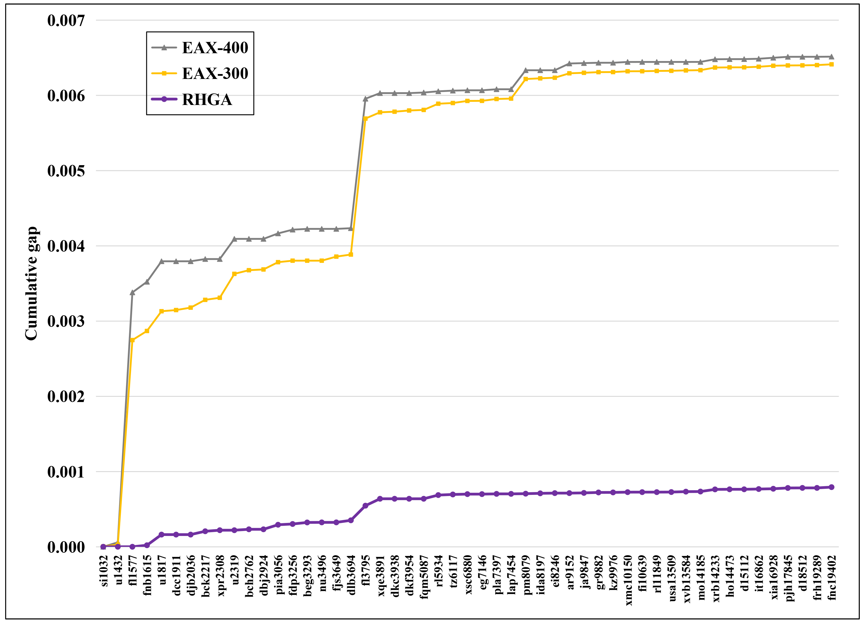
(a) Cumulative gap on 51 small but not easy instances.

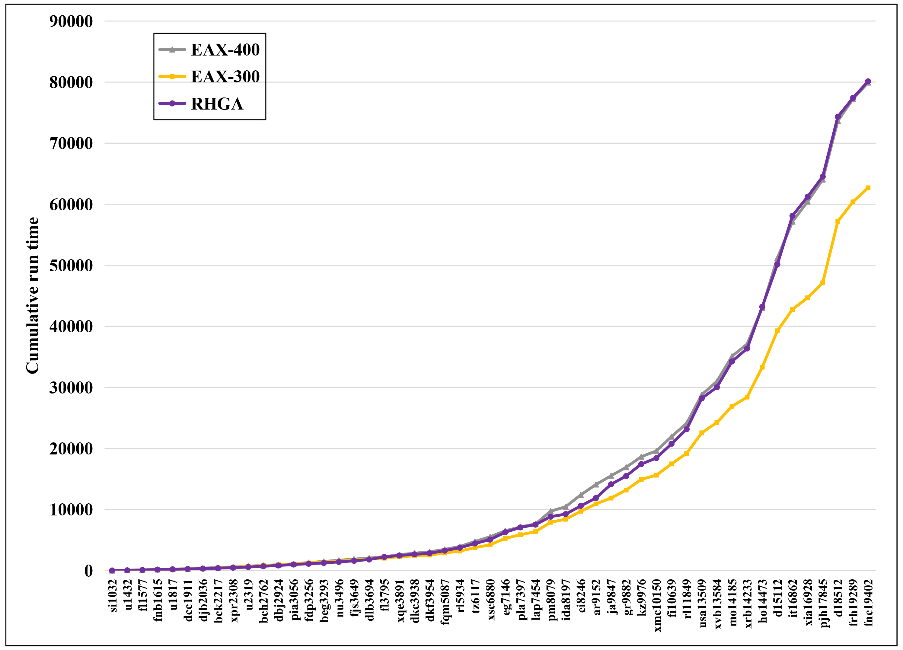
(b) Cumulative run time on 51 small but not easy instances.

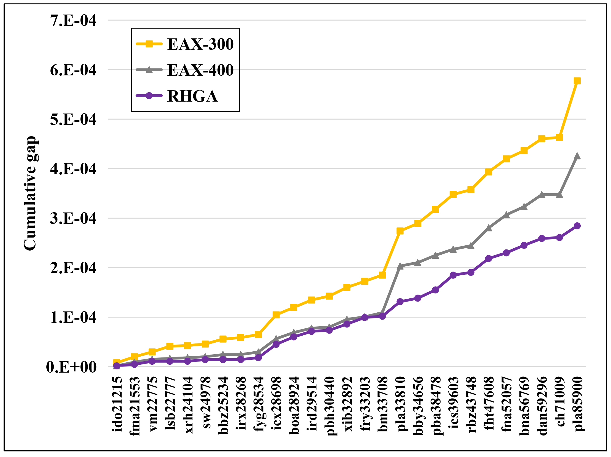
(c) Cumulative gap on 27 large instances.

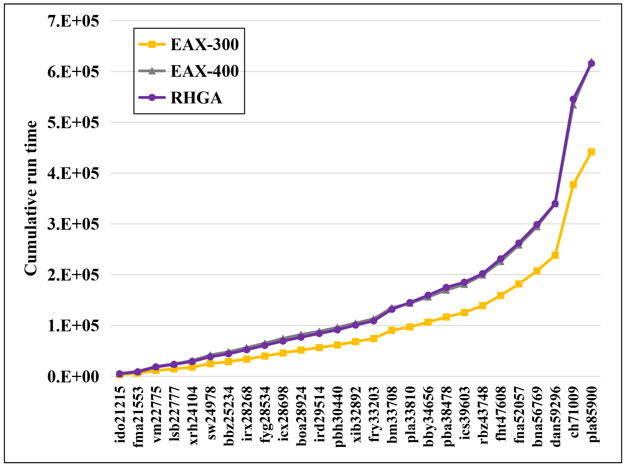
(d) Cumulative run time on large instances.

Figure 1: Comparison results of RHGA, EAX-300 and EAX-400 in solving the 51 small but not easy instances and 27 large instances.

5.1 Various Variants of the Algorithm

We first present various variant algorithms of RHGA and EAX-GA for comparison and analysis. The variant algorithms include the following:

• Alpha-EAX: A variant of EAX-300 using the $\alpha$-value (Eq. 1) to replace the distance metric used in the process of merging sub-tours in EAX-300 (see Step 5 in Section 2.2).

• FixQ-EAX: A variant of EAX-300 using the initial Q-value (Eq. 2) to replace the distance metric used in the process of merging sub-tours in EAX-300.

• Q-EAX: A variant of EAX-300 using the adaptive Q-value learned by the Q-learning method (Eq. 3) to replace the distance metric used in the process of merging sub-tours in EAX-300. The population size in Q-EAX is set to be 301. The extra individual is the special individual used to learn the Q-value and provide the adaptive Q-value for the algorithm. The special individual in Q-EAX can be improved by the Q-LKH local search and the genetic algorithm, but other individuals cannot be improved by crossing with the special individual (i.e., the special individual in Q-EAX can only be $p_{A}$, not $p_{B}$). In addition, the result of Q-EAX is the best individual in the population except for the special individual, and Q-EAX will not terminate if the special individual is the optimum solution (if known).

• Q-EAX+Special: A variant of Q-EAX that the output is the best individual in the population includes the special individual. Q-EAX+Special terminates when the special individual is the optimum solution. In a word, the difference between Q-EAX+Special and Q-EAX includes: 1) whether the special individual can be the output solution. 2) Whether the algorithm terminates when the special individual is the optimum solution.

• EAX-LKH: A variant of RHGA that combines EAX-GA with the LKH algorithm as RHGA does but with no reinforcement learning. The metrics in the EAX-GA and LKH local search are not changed.

• Alpha-EAX-LKH: A variant of EAX-LKH using the $\alpha$-value (Eq. 1) to replace the distance metric in EAX-GA.

• FixQ-EAX-LKH: A variant of EAX-LKH using the initial Q-value (Eq. 2) to replace the distance metric in EAX-GA and the $\alpha$-value metric in LKH.

• RHGA-$k$: A variant of RHGA that the number of the special individuals is $k$ (we tested $k=3,5,20,50$ in experiments). Each special individual $x_{i}$, $i\leq{k}$, can be improved by Q-LKH when: 1) it is just initialized, or it was improved by EAX-GA at the last generation. In this case, Q-LKH will try to improve $x_{i}$. 2) It has not been improved for $M_{gen}$ generations, and the algorithm randomly selects an individual $x_{r}$ ($x_{r}$ is not a special individual). If $x_{r}$ can be improved by Q-LKH and the improved tour is better than $x_{i}$, then replace $x_{i}$ with the improved tour. Moreover, when the best individual $x_{best}$ in the population besides the $k$ special individuals is better than the best special individual and $x_{best}$ has not been calculated by Q-LKH, Q-LKH will try to improve $x_{best}$. The improved tour will replace $x_{1}$ (do not replace $x_{1}$ if $x_{best}$ cannot be improved by Q-LKH).

The termination conditions of all the above algorithms are the same as in RHGA. Since the calculation time of RHGA is a little longer than EAX-300 and close to EAX-400 when solving the tested benchmarks, the calculation times of the variant algorithms, including Alpha-EAX, FixQ-EAX, Q-EAX, Q-EAX+Special, EAX-LKH, Alpha-EAX-LKH, FixQ-EAX-LKH, are also roughly between that of EAX-300 and EAX-400.

We further introduce three hybrid algorithms that combine EAX-GA with LKH in a straightforward manner:

• Min{EAX, LKH}: Given an input instance, this algorithm first uses EAX-GA and LKH to calculate the instance 10 times respectively, and then selects the one with the better average solution as the output.

• LKH+EAX: A hybrid algorithm that uses LKH to generate the initial population, and then runs EAX-GA starting from this population.

• EAX+LKH: A hybrid algorithm that first uses EAX-GA to calculate the input instance until the termination conditions of EAX-GA are reached (or the known optimum is obtained), then runs LKH with its initial solution equal to the best individual. The LKH algorithm in EAX+LKH terminates as EAX-GA does. That is, let $Gen$ be the number of iterations at which no improvement in the best solution is found by LKH over the recent $1500/N_{ch}$ iterations. If $Gen$ has been determined and the best solution does not improve over the last $G_{max}=Gen/10$ iterations, EAX+LKH terminates.

5.2 Analysis on the Combination Mechanism of RHGA

In order to demonstrate that our proposed combination mechanism is reasonable and effective, we first compare EAX-LKH with the hybrid algorithms Min{EAX, LKH}, LKH+EAX, and EAX+LKH, as well as the baselines EAX-300 and EAX-400 on all the 51 small but not easy instances in Figure 2(a). We also present the results without LKH+EAX in Figure 2(b) for a clearer comparison.

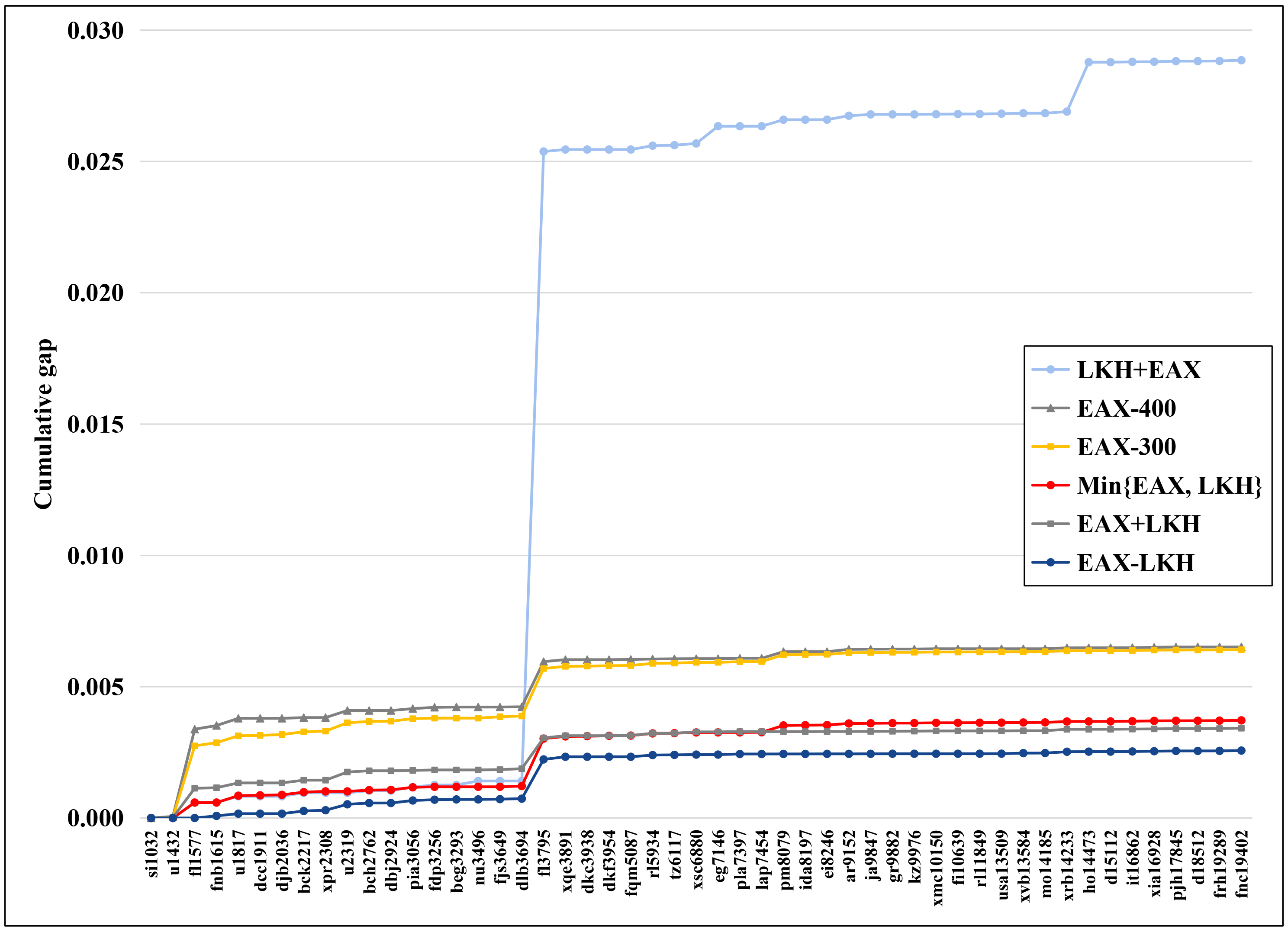
(a) Comparison results with LKH+EAX.

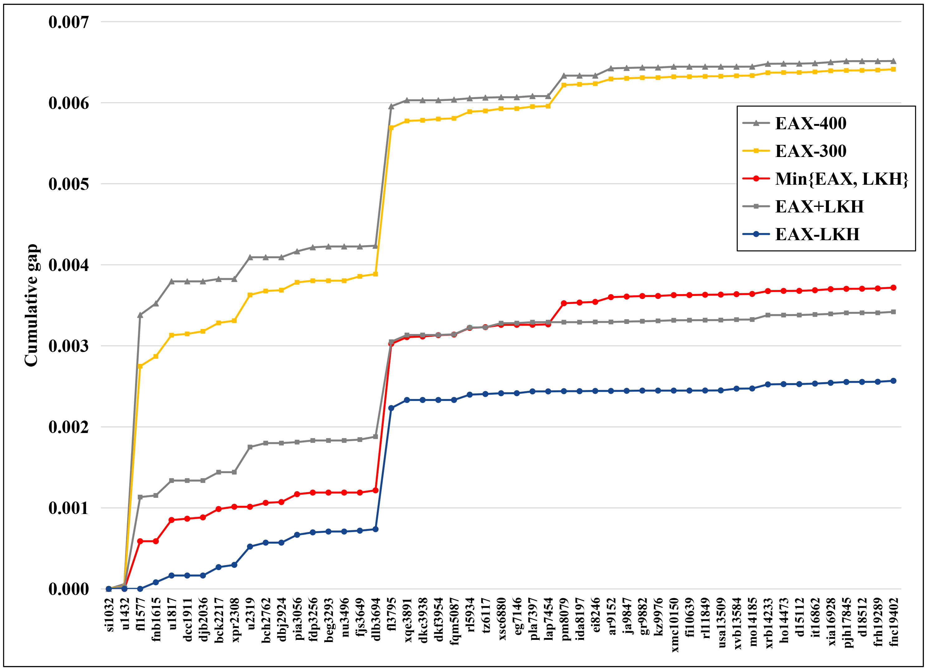
(b) Comparison results without LKH+EAX.

Figure 2: Analysis on the combination mechanism on 51 small but not easy instances.

As shown in Figure 2, LKH+EAX is much worse than EAX-300 and EAX-400. Note that the method to generate the initial population in EAX-GA is a simple greedy 2-opt local search [3]. Why does LKH+EAX use the effective LKH local search to replace the simple 2-opt results in much worse performance? The reason is that the initial population of LKH+EAX contains too many candidate edges provided by LKH. Thus the population diversity is broken and it is easy for the algorithm to get stuck in local optima. In this case, if LKH can provide good genes, i.e., the edges in the optimal solution are contained in the candidate edges, LKH+EAX can obtain better results than EAX-GA. Otherwise, its performance is poor. The results in Figure 2 can demonstrate this comment, as the performance of LKH+EAX mainly depends on LKH. For the instances that LKH works well (see detailed results of LKH in Tables 2, 3, and 4), such as u1432 and u2319, LKH+EAX shows better performance than EAX-300 and EAX-400. For the instances that LKH can not work well, such as fl3795, eg7146, and ho14472. LKH+EAX shows much worse performance than EAX-300 and EAX-400. This result can also demonstrate that our mechanism that only one special individual can be improved by LKH is reasonable.

Moreover, algorithms Min{EAX, LKH} and EAX+LKH can surely obtain results no worse than EAX-GA, because they can obtain at least the same solution as EAX-GA does. However, the straightforward combinations of EAX-GA and LKH can not make full use of their complementary, as the EAX-LKH algorithm with our combination mechanism shows much better performance than Min{EAX, LKH} and EAX+LKH. Note that Min{EAX, LKH} can be regarded as the hybrid solver proposed by Kerschke et al. [15] consists of EAX-GA and LKH with a perfect prediction model. Therefore, the combination mechanism in RHGA is much more effective than the straightforward hybrid mechanisms we designed for comparison and the hybrid mechanism proposed by Kerschke et al. [15], and can make better use of the complementary of EAX-GA and LKH.

5.3 Analysis on Different Metrics and the Special Individual

We then compare RHGA with the variant algorithms to evaluate the performance of different metrics in determining the candidate edges, and evaluate the effectiveness of the special individual in RHGA. Figure 3(a) compares the results of 10 different algorithms, including RHGA, Alpha-EAX, FixQ-EAX, Q-EAX, Q-EAX+Special, EAX-LKH, Alpha-EAX-LKH, FixQ-EAX-LKH, EAX-300, and EAX-400, on the same 51 instances in Figure 2. We also present the results without EAX-300 and EAX-400 in Figure 3(b) for a clearer comparison.

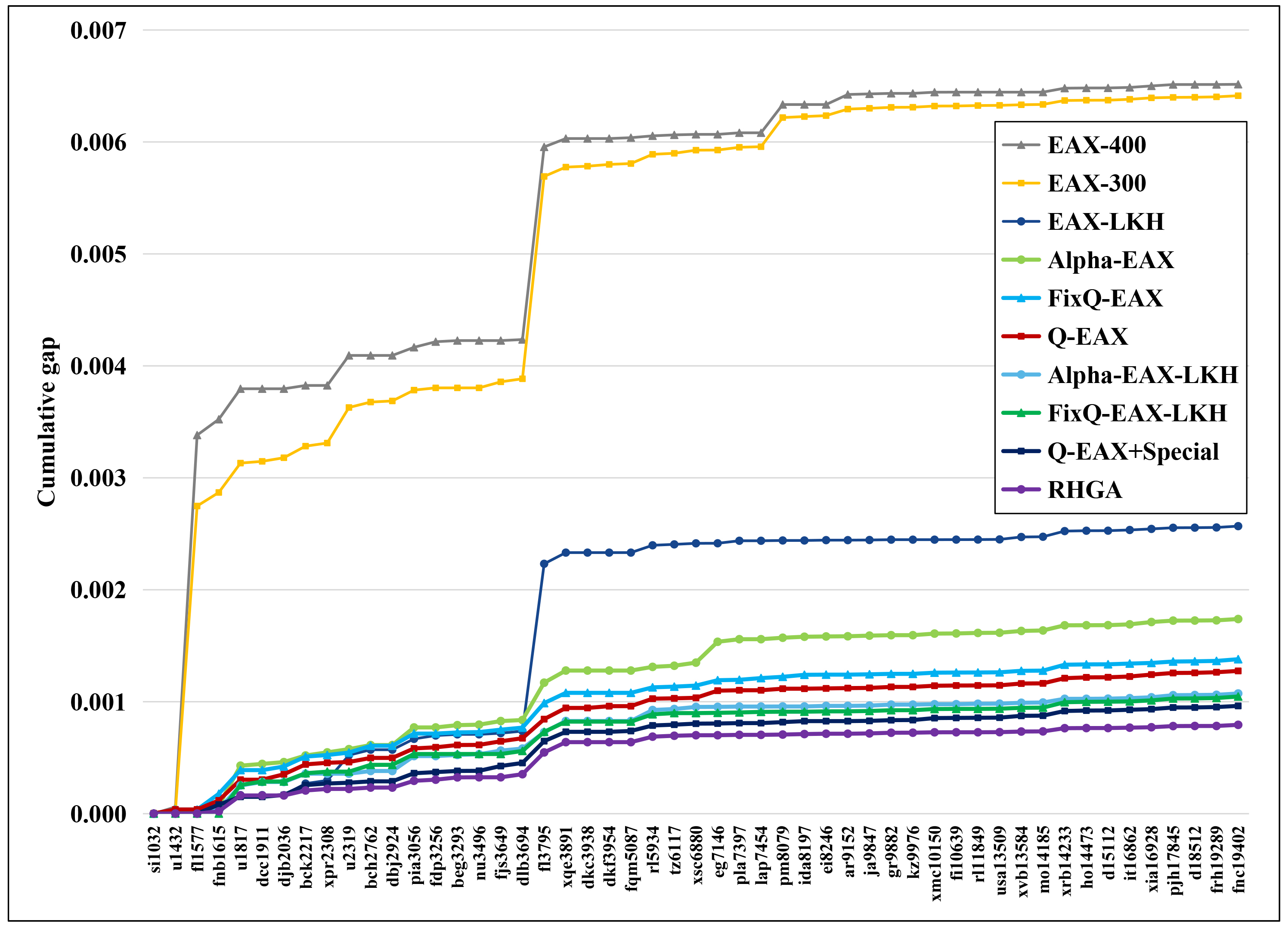
(a) Comparison results with EAX-300 and EAX-400.

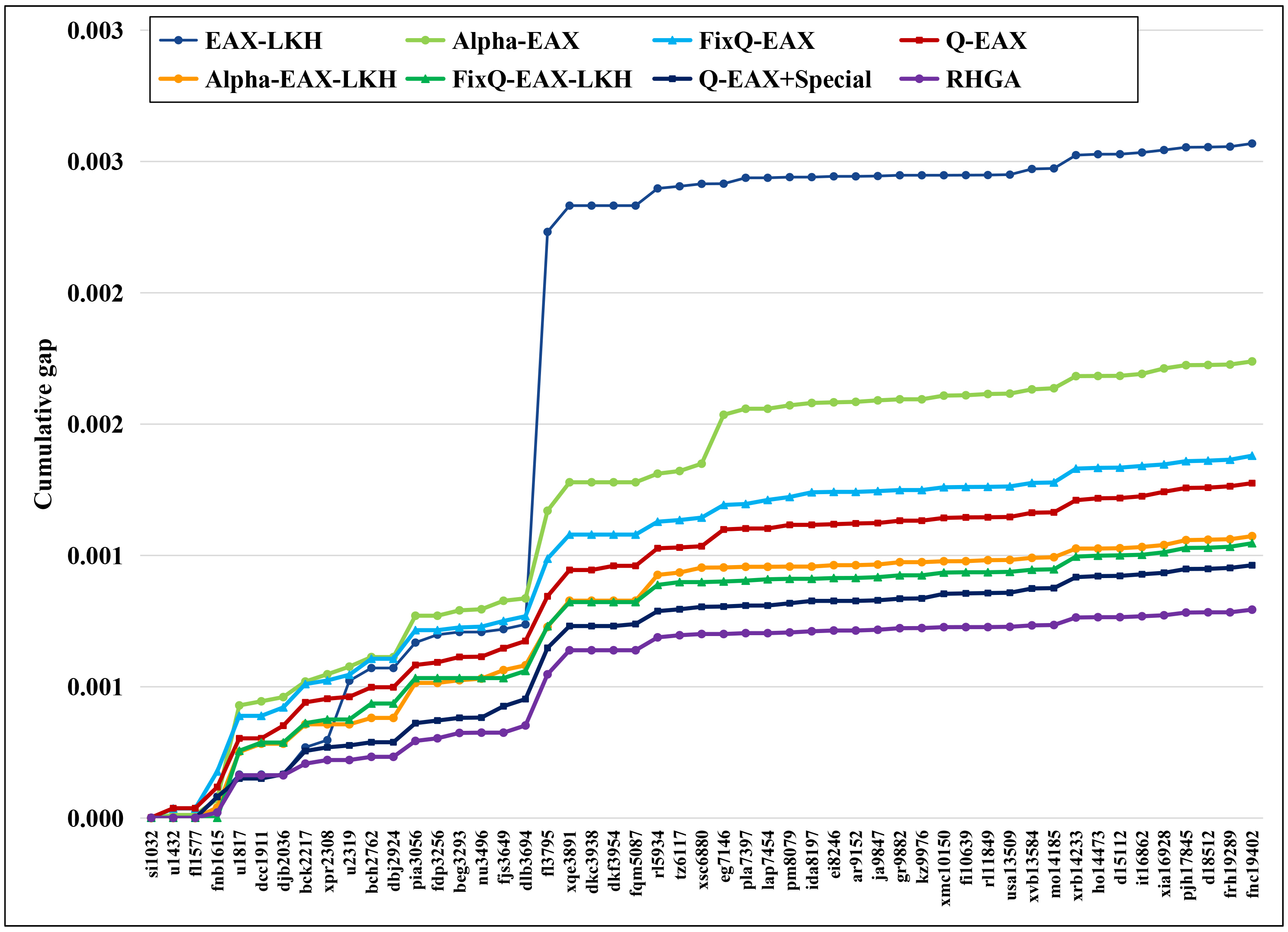
(b) Comparison results without EAX-300 and EAX-400.

Figure 3: Analysis on different metrics and the special individual on 51 small but not easy instances.

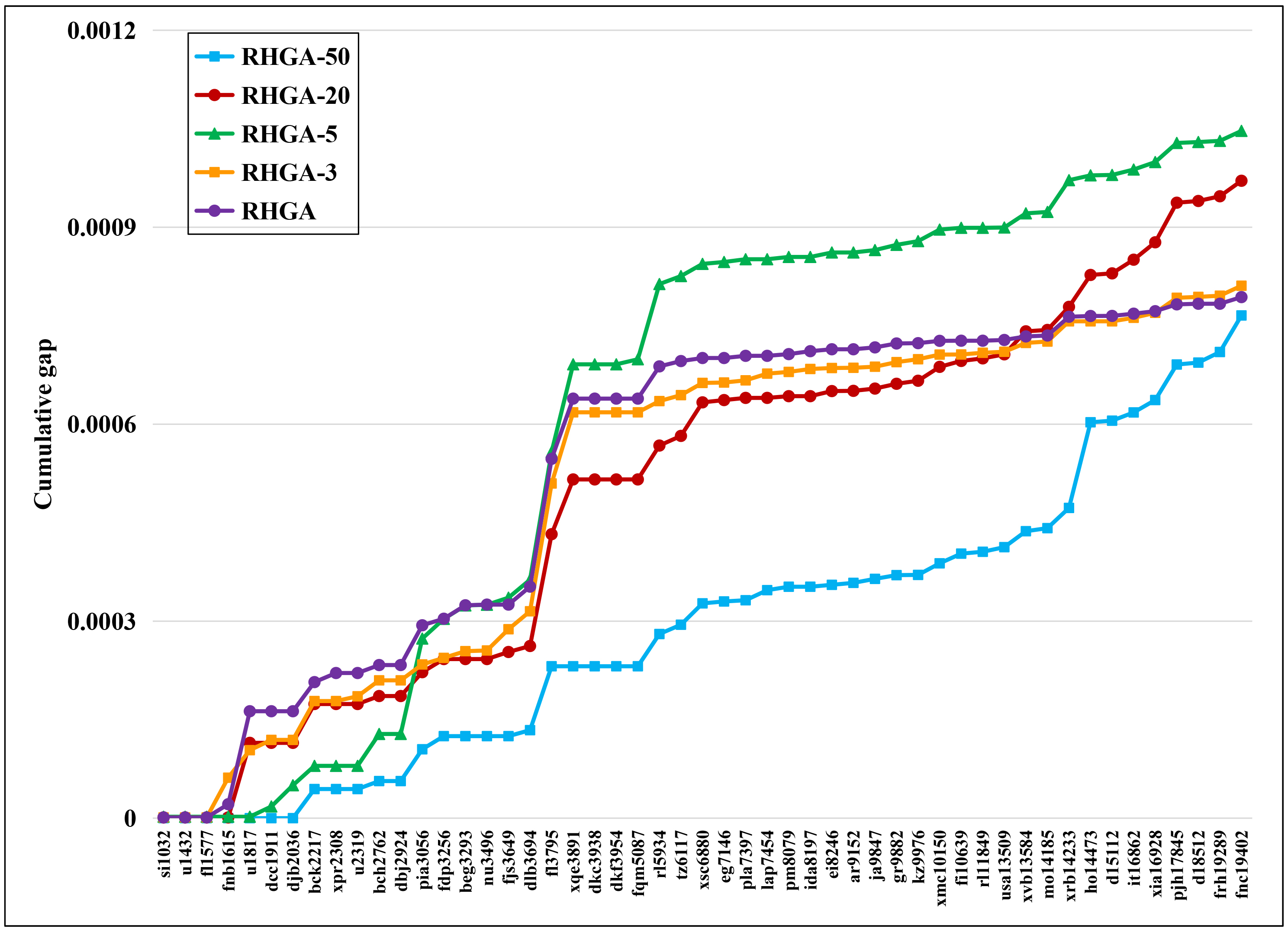
(a) Comparison on cumulative gap.

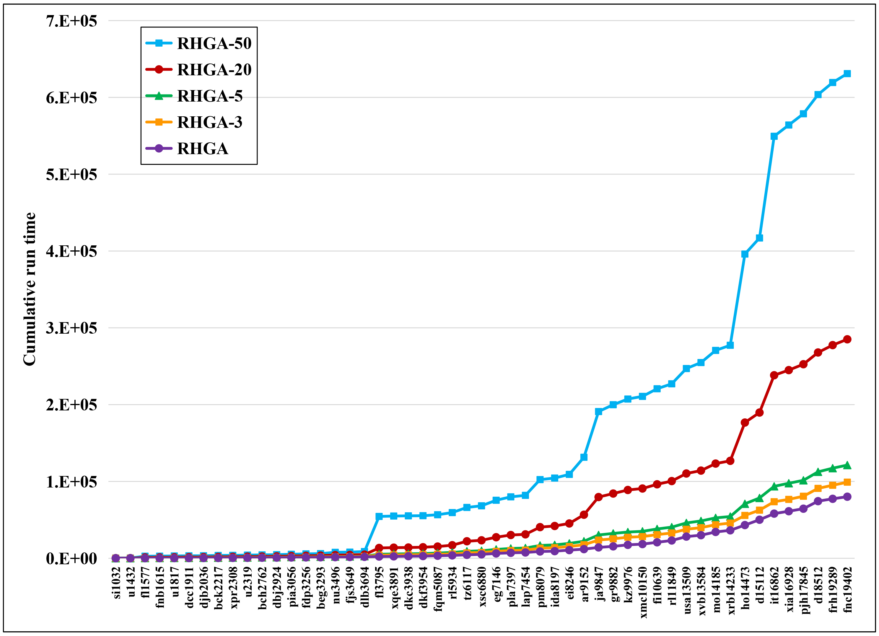
(b) Comparison on cumulative run time.

Figure 4: Comparison results of RHGA and RHGA-3/5/20/50 in solving the 51 small but not easy instances.

The results of EAX-LKH, Alpha-EAX-LKH, FixQ-EAX-LKH, and RHGA in Figure 3 indicate that, the order with decaying quality of the performance of different metrics is: adaptive Q-value (updated by reinforcement learning according to Eq. 3), initial Q-value (Eq. 2), $\alpha$-value and distance. The results of EAX-300, Alpha-EAX, FixQ-EAX, and Q-EAX can draw the same conclusion. As a result, the EAX-GA algorithm can be improved simply by replacing the distance metric with the $\alpha$-value or initial Q-value, and reinforcement learning can further improve the performance of the initial Q-value. Moreover, the combination of EAX-GA and LKH by our proposed mechanism is always effective, since EAX-LKH/Alpha-EAX-LKH/FixQ-EAX-LKH/RHGA outperforms EAX-300/Alpha-EAX/FixQ-EAX/Q-EAX significantly.

The results of Q-EAX, Q-EAX+Special, and RHGA in Figure 3 can further lead to the following comments. First, Q-EAX+Special outperforms Q-EAX, indicating that the special individual can provide better solutions than the other individuals. Second, RHGA outperforms Q-EAX+Special, indicating that the special individual can also improve the population by spreading its genes to other individuals. In summary, the benefits of the special individual are as follows: 1) it can provide the adaptive Q-value for the EAX-GA to improve the performance. 2) it can obtain good solutions since it can be improved by both Q-LKH and EAX-GA (when $x_{1}$ is parent $p_{A}$). 3) it can improve the population by providing its high-quality genes for other individuals (when $x_{1}$ is parent $p_{B}$).

5.4 Comparison with Multiple Special Individuals

We then compare RHGA with the RHGA-$k$ algorithms, including RHGA-3, RHGA-5, RHGA-20, and RHGA-50, on the same 51 instances in Figure 2, to analyze the influence of the number of special individuals on the performance. The comparison results are shown in Figure 4.

From the results we can observe that:

(1) RHGA and RHGA-3 show similar performance in solving the 51 instances. The algorithms with a larger number of special individuals show better performance in solving the instances with relatively small scales. For example, the RHGA-5 is good at solving the instances with less than 3,000 cities, and the RHGA-20 and RHGA-50 are good at solving the instances with less than 6,000 cities. However, neither of the three algorithms with a larger number of special individuals is good at solving the instances with larger than 14,000 cities, indicating that for solving relatively large and complex instances, an excessive proportion of special individuals in the population may reduce the algorithm performance.

(2) The calculation time of the RHGA-$k$ algorithm increases rapidly as $k$ increases. Specifically, the calculation time of RHGA-3/5/20/50 is about 24/51/256/687% more than that of RHGA.

In summary, setting multiple special individuals in the population is not reasonable and time-consuming. Thus it is suitable and effective to set only one special individual in the population, which can help the algorithm obtain a good performance without reducing the efficiency.

6 Conclusion

In this paper, we address the famous NP-hard traveling salesman problem and propose a reinforced hybrid genetic algorithm (RHGA) that combines reinforcement learning with two state-of-the-art heuristic algorithms, the EAX-GA genetic algorithm and the LKH local search heuristic, in a more interactive form. The EAX-GA and LKH are integrated with the help of a special and unique individual, which can be improved by both the genetic algorithm and the local search algorithm. In our proposed hybrid mechanism, the population provides diverse and high-quality initial solutions for the LKH local search algorithm, and the local search algorithm leads the population to converge to better results. In a word, the two state-of-the-art TSP heuristics, EAX-GA and LKH, can boost each other in our proposed hybrid mechanism. Moreover, the Q-learning algorithm is applied to learn an adaptive Q-value to replace the distance metric used in the process of merging sub-tours in EAX-GA and the $\alpha$-value used in LKH for determining the candidate cities. As a result, our reinforcement learning method can improve both the EAX-GA and the LKH algorithms by providing better candidate edges.

Extensive experimental results demonstrate that RHGA outperforms the powerful EAX-GA and LKH algorithms, as well as one of the state-of-the-art (deep) learning based algorithms, NeuroLKH, for solving the TSP. Further and extensive ablation studies are adopted to show the effectiveness of the proposed hybrid mechanism and the reinforcement learning method, and to demonstrate that the proposed hybrid mechanism can make full use of the complementary of EAX-GA and LKH, and the setting of only one special individual is reasonable and efficient.

In future work, the proposed mechanism of combining genetic algorithms with local search could be applied to solve various combinatorial optimization problems, and the method of combining reinforcement learning with the core process of heuristics would also be applied to improve other heuristic algorithms.

References

- [1] Elias B. Khalil, Hanjun Dai, Yuyu Zhang, Bistra Dilkina, and Le Song. Learning combinatorial optimization algorithms over graphs. In Annual Conference on Neural Information Processing Systems 2017, NIPS 2017, pages 6348–6358, 2017.
- [2] Keld Helsgaun. An effective implementation of the lin-kernighan traveling salesman heuristic. European Journal of Operational Research, 126(1):106–130, 2000.
- [3] Yuichi Nagata and Shigenobu Kobayashi. A powerful genetic algorithm using edge assembly crossover for the traveling salesman problem. INFORMS Journal on Computing, 25(2):346–363, 2013.
- [4] Shen Lin and Brian W. Kernighan. An effective heuristic algorithm for the traveling-salesman problem. Operations Research, 21(2):498–516, 1973.
- [5] Huai-Kuang Tsai, Jinn-Moon Yang, Yuan-Fang Tsai, and Cheng-Yan Kao. An evolutionary algorithm for large traveling salesman problems. IEEE Transactions on Systems, Man, and Cybernetics, Part B, 34(4):1718–1729, 2004.
- [6] Yuichi Nagata and Shigenobu Kobayashi. Edge assembly crossover: A high-power genetic algorithm for the travelling salesman problem. In The Seventh International Conference on Genetic Algorithms, ICGA 1997, pages 450–457, 1997.
- [7] Nico LJ Ulder, Emile HL Aarts, Hans-Jürgen Bandelt, Peter JM Van Laarhoven, and Erwin Pesch. Genetic local search algorithms for the traveling salesman problem. In International Conference on Parallel Problem Solving from Nature, PPSN 1990, volume 496, pages 109–116, 1990.
- [8] Bernd Freisleben and Peter Merz. New genetic local search operators for the traveling salesman problem. In Parallel Problem Solving from Nature - PPSN IV, International Conference on Evolutionary Computation. The Fourth International Conference on Parallel Problem Solving from Nature, PPSN 1996, volume 1141, pages 890–899, 1996.
- [9] Peter Merz and Bernd Freisleben. Genetic local search for the tsp: new results. In IEEE International Conference on Evolutionary Computation, ICEC 1997, pages 159–164, 1997.
- [10] Hung Dinh Nguyen, Ikuo Yoshihara, Kunihito Yamamori, and Moritoshi Yasunaga. Implementation of an effective hybrid GA for large-scale traveling salesman problems. IEEE Transactions on Systems, Man, and Cybernetics, Part B, 37(1):92–99, 2007.
- [11] L. Darrell Whitley, Doug Hains, and Adele E. Howe. A hybrid genetic algorithm for the traveling salesman problem using generalized partition crossover. In Parallel Problem Solving from Nature - PPSN XI, Eleventh International Conference, Part I, PPSN I 2010, volume 6238, pages 566–575, 2010.
- [12] Yong Wang. The hybrid genetic algorithm with two local optimization strategies for traveling salesman problem. Computers & Industrial Engineering, 70:124–133, 2014.
- [13] Mohammad Harun Rashid and Miguel A. Mosteiro. A greedy-genetic local-search heuristic for the traveling salesman problem. In 2017 IEEE International Symposium on Parallel and Distributed Processing with Applications and 2017 IEEE International Conference on Ubiquitous Computing and Communications, ISPA/IUCC 2017, pages 868–872, 2017.
- [14] Vladimir Ilin, Dragan Simic, Svetislav D. Simic, and Svetlana Simic. Hybrid genetic algorithms and tour construction and improvement algorithms used for optimizing the traveling salesman problem. In Fifteenth International Conference on Soft Computing Models in Industrial and Environmental Applications, SOCO 2020, volume 1268, pages 530–539, 2020.
- [15] Pascal Kerschke, Lars Kotthoff, Jakob Bossek, Holger H. Hoos, and Heike Trautmann. Leveraging TSP solver complementarity through machine learning. Evolutionary Computation, 26(4), 2018.
- [16] Richard S. Sutton and Andrew G. Barto. Reinforcement learning - an introduction. Adaptive computation and machine learning. MIT Press, 1998.
- [17] Yujiao Hu, Yuan Yao, and Wee Sun Lee. A reinforcement learning approach for optimizing multiple traveling salesman problems over graphs. Knowledge-Based Systems, 204:106244, 2020.
- [18] Ajani S. Oladayo and Rammohan Mallipeddi. Adaptive evolution strategy with ensemble of mutations for reinforcement learning. Knowledge-Based Systems, 245:108624, 2022.
- [19] Jiongzhi Zheng, Kun He, Jianrong Zhou, Yan Jin, and Chu-min Li. Combining reinforcement learning with lin-kernighan-helsgaun algorithm for the traveling salesman problem. In Thirty-Fifth AAAI Conference on Artificial Intelligence, AAAI 2021, pages 12445–12452, 2021.
- [20] Yoshua Bengio, Andrea Lodi, and Antoine Prouvost. Machine learning for combinatorial optimization: A methodological tour d’horizon. European Journal of Operational Research, 290(2):405–421, 2021.
- [21] Irwan Bello, Hieu Pham, Quoc V. Le, Mohammad Norouzi, and Samy Bengio. Neural combinatorial optimization with reinforcement learning. In Fitth International Conference on Learning Representations, Workshop Track Proceedings, ICLR (Workshop) 2017, 2017.
- [22] Oriol Vinyals, Meire Fortunato, and Navdeep Jaitly. Pointer networks. In Annual Conference on Neural Information Processing Systems 2015, NIPS 2015, pages 2692–2700, 2015.
- [23] Yong Liang Goh, Wee Sun Lee, Xavier Bresson, Thomas Laurent, and Nicholas Lim. Combining reinforcement learning and optimal transport for the traveling salesman problem. CoRR, abs/2203.00903, 2022.
- [24] Marco Cuturi. Sinkhorn distances: Lightspeed computation of optimal transport. In Annual Conference on Neural Information Processing Systems 2013., pages 2292–2300, 2013.
- [25] Patrick Emami and Sanjay Ranka. Learning permutations with sinkhorn policy gradient. CoRR, abs/1805.07010, 2018.
- [26] Fei Liu and Guangzhou Zeng. Study of genetic algorithm with reinforcement learning to solve the TSP. Expert Systems with Applications, 36(3):6995–7001, 2009.
- [27] Yuichi Nagata. New EAX crossover for large TSP instances. In Parallel Problem Solving from Nature - PPSN IX, Ninth International Conference, PPSN 2006, volume 4193, pages 372–381, 2006.
- [28] Paulo R. de O. da Costa, Jason Rhuggenaath, Yingqian Zhang, and Alp Akcay. Learning 2-opt heuristics for the traveling salesman problem via deep reinforcement learning. In The Twelfth Asian Conference on Machine Learning, ACML 2020, volume 129, pages 465–480, 2020.
- [29] Jingyan Sui, Shizhe Ding, Ruizhi Liu, Liming Xu, and Dongbo Bu. Learning 3-opt heuristics for traveling salesman problem via deep reinforcement learning. In The Thirteenth Asian Conference on Machine Learning, ACML 2021, volume 157, pages 1301–1316, 2021.
- [30] Jiuxia Zhao, Minjia Mao, Xi Zhao, and Jianhua Zou. A hybrid of deep reinforcement learning and local search for the vehicle routing problems. IEEE Transactions on Intelligent Transportation Systems, 22(11):7208–7218, 2021.
- [31] Liang Xin, Wen Song, Zhiguang Cao, and Jie Zhang. Neurolkh: Combining deep learning model with lin-kernighan-helsgaun heuristic for solving the traveling salesman problem. In Annual Conference on Neural Information Processing Systems 2021, NeurIPS 2021, pages 7472–7483, 2021.
- [32] Keiji Maekawa, Naoki Mori, Hisashi Tamaki, Hajime Kita, and Yoshikazu Nishikawa. A genetic solution for the traveling salesman problem by means of a thermodynamical selection rule. In IEEE International Conference on Evolutionary Computation, ICEC 1996, pages 529–534, 1996.
- [33] Shen Lin. Computer solutions of the traveling salesman problem. Bell System Technical Journal, 44(10):2245–2269, 1965.
- [34] Michael Held and Richard M. Karp. The traveling-salesman problem and minimum spanning trees. Operations Research, 18(6):1138–1162, 1970.
- [35] Keld Helsgaun. General k-opt submoves for the lin-kernighan TSP heuristic. Mathematical Programming Computation, 1(2-3):119–163, 2009.