KUNS-2885, YITP-21-75

Statistical analysis method for the worldvolume hybrid Monte Carlo algorithm

Masafumi Fukuma¹, Nobuyuki Matsumoto² and Yusuke Namekawa³

¹Department of Physics, Kyoto University, Kyoto 606-8502, Japan ²RIKEN/BNL Research center, Brookhaven National Laboratory, Upton, NY 11973, USA ³Yukawa Institute for Theoretical Physics, Kyoto University, Kyoto 606-8502, Japan

We discuss the statistical analysis method for the worldvolume hybrid Monte Carlo (WV-HMC) algorithm [arXiv:2012.08468], which was recently introduced to substantially reduce the computational cost of the tempered Lefschetz thimble method. In the WV-HMC algorithm, the configuration space is a continuous accumulation (worldvolume) of deformed integration surfaces, and sample averages are considered for various subregions in the worldvolume. We prove that, if a sample in the worldvolume is generated as a Markov chain, then the subsample in the subregion can also be regarded as a Markov chain. This ensures the application of the standard statistical techniques to the WV-HMC algorithm. We particularly investigate the autocorrelation times for the Markov chains in various subregions, and find that there is a linear relation between the probability to be in a subregion and the autocorrelation time for the corresponding subsample. We numerically confirm this scaling law for a chiral random matrix model.

1 Introduction

The numerical sign problem has prevented us from the first-principles analysis of various important systems, such as quantum chromodynamics (QCD) at finite density [1], quantum Monte Carlo calculations of quantum statistical systems [2], and the real-time dynamics of quantum fields.

Among various approaches to the sign problem, some utilize the complexification of dynamical variables. For example, in the complex Langevin method [3, 4, 5, 6], one considers the Langevin equation in the complexified configuration space. In the path optimization method [7, 8, 9, 10], with the aid of machine learning one looks for an optimized integration surface for which the average phase factor is maximal. In the Lefschetz thimble method [11, 12, 13, 14, 15, 16, 17, 18, 19, 20, 21, 22, 23], one deforms the integration surface according to the antiholomorphic gradient flow. The deformed surface asymptotes to a union of Lefschetz thimbles, each of which gives a constant value to the imaginary part of the action and thus is free from the sign problem. Although there can appear the ergodicity problem due to the existence of infinitely high potential barriers between thimbles, this ergodicity problem can be diminished by tempering the system with the flow time [19]. This tempered Lefschetz thimble method (TLTM) thus solves the sign and ergodicity problems simultaneously. Moreover, the computational cost of TLTM has recently been reduced significantly by developing the worldvolume tempered Lefschetz thimble method (WV-TLTM) [23], which we are going to review now.

Let ${\mathbb{R}}^{N}=\{x\}$ be the configuration space and $S(x)$ the action (allowed to be complex-valued). Our main interest is to numerically estimate the expectation values of observables $\mathcal{O}(x)$,

$$\langle\mathcal{O}\rangle\equiv\frac{\int_{{\mathbb{R}}^{N}}dx\,e^{-S(x)}\,\mathcal{O}(x)}{\int_{{\mathbb{R}}^{N}}dx\,e^{-S(x)}}.$$ (1.1)

Under the assumption that $e^{-S(z)}$ and $e^{-S(z)}\,\mathcal{O}(z)$ are entire functions of $z\in{\mathbb{C}}^{N}$, Cauchy’s theorem allows us to continuously deform the integration surface without changing the value of integral. By expressing the deformation as a flow $z_{t}(x)$ $(t\geq 0)$ with $z_{0}(x)=x$, the deformed integration surface at flow time $t$ can be written as $\Sigma_{t}=\{z_{t}(x)\,|\,x\in{\mathbb{R}}^{N}\}$, and thus we have the equality

$$\langle\mathcal{O}\rangle=\frac{\int_{\Sigma_{t}}dz_{t}\,e^{-S(z_{t})}\,\mathcal{O}(z_{t})}{\int_{\Sigma_{t}}dz_{t}\,e^{-S(z_{t})}}.$$ (1.2)

Since the numerator and the denominator are both independent of $t$, we can integrate each of them over an arbitrary interval $[T_{0},T_{1}]$ with an arbitrary function $W(t)$. This rewrites (1.2) to the integration over the worldvolume $\mathcal{R}\equiv\bigcup_{T_{0}\leq t\leq T_{1}}\Sigma_{t}$:

$$\langle\mathcal{O}\rangle=\frac{\int_{T_{0}}^{T_{1}}dt\,e^{-W(t)}\int_{\Sigma_{t}}dz_{t}\,e^{-S(z_{t})}\,\mathcal{O}(z_{t})}{\int_{T_{0}}^{T_{1}}dt\,e^{-W(t)}\int_{\Sigma_{t}}dz_{t}\,e^{-S(z_{t})}}=\frac{\int_{\mathcal{R}}Dz\,K(z)\,e^{-W(t(z))}\,e^{-S(z)}\,\mathcal{O}(z)}{\int_{\mathcal{R}}Dz\,K(z)\,e^{-W(t(z))}\,e^{-S(z)}},$$ (1.3)

where $Dz$ is the induced volume element on $\mathcal{R}$, and $K(z)$ is the Jacobian: $dt\,dz_{t}=K(z)\,Dz$. The weight factor $e^{-W(t)}$ is chosen so that the probability for a configuration to appear at time $t$ is (almost) independent of $t$. This setting is especially necessary when the whole range of $t$ is relevant to simulations, as in the WV-TLTM. We further rewrite (1.3) to the ratio of reweighted averages:

$$\langle\mathcal{O}\rangle=\frac{\int_{\mathcal{R}}Dz\,e^{-V(z)}\,A(z)\,\mathcal{O}(z)}{\int_{\mathcal{R}}Dz\,e^{-V(z)}\,A(z)}=\frac{\langle A(z)\,\mathcal{O}(z)\rangle_{\mathcal{R}}}{\langle A(z)\rangle_{\mathcal{R}}}.$$ (1.4)

Here, the reweighted average

$$\langle\mathcal{O}(z)\rangle_{\mathcal{R}}\equiv\frac{\int_{\mathcal{R}}Dz\,e^{-V(z)}\,\mathcal{O}(z)}{\int_{\mathcal{R}}Dz\,e^{-V(z)}}$$ (1.5)

is defined for the weight $e^{-V(z)}\equiv e^{-{\rm Re}\,S(z)-W(t(z))}$, and $A(z)$ is the reweighting factor

$$A(z)\equiv\frac{e^{-S(z)-W(t(z))}dt\,dz_{t}}{e^{-V(z)}Dz}=e^{-i\,{\rm Im}\,S(z)}K(z),$$ (1.6)

whose explicit form can be found in Ref. [23].

The reweighted average (1.5) is estimated by the average over a sample generated by the hybrid Monte Carlo (HMC) algorithm with the potential $V(z)$. We will generally call a HMC algorithm on an accumulation of integration surfaces the worldvolume hybrid Monte Carlo algorithm (the WV-HMC algorithm), which includes the WV-TLTM.

In the case of the WV-TLTM, the interval $[T_{0},T_{1}]$ should include the region with large $t$ so as to solve the sign problem, and at the same time include the region with small $t$ so as to reduce the ergodicity problem. However, the small-$t$ region may be contaminated by the sign problem, and the large-$t$ region by the ergodicity problem. Thus, in order to reduce the contributions from these potentially contaminated regions, it was proposed in Ref. [23] to estimate the observables from a subsample in a subregion with $[\tilde{T}_{0},\tilde{T}_{1}]$ ($\subset[T_{0},T_{1}]$) (see Fig. 1), where $\tilde{T}_{0}$ and $\tilde{T}_{1}$ are chosen such that the estimated values vary only slightly against the changes of $\tilde{T}_{0}$ and $\tilde{T}_{1}$.

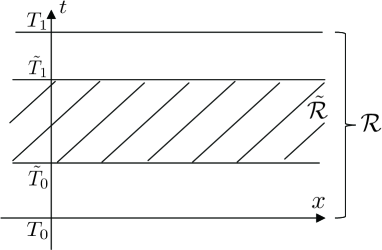
Figure 1: The worldvolume $\mathcal{R}$ and a subregion $\tilde{\mathcal{R}}$.

In Ref. [23] the standard error analysis was employed as if the subsample itself is generated as a Markov chain with ergodicity and detailed balance. However, this is not obvious and needs a justification. In this paper, we prove that, if consecutive configurations in the worldvolume are generated as a Markov chain with ergodicity and detailed balance, then the subset consisting of the configurations belonging to a subregion can also be regarded as a Markov chain with ergodicity and detailed balance intact. We particularly investigate the integrated autocorrelation times for the Markov chains in various subregions, and find that there is a linear relation between the probability to be in a subregion and the integrated autocorrelation time for the corresponding subsample. We numerically confirm this scaling law for a chiral random matrix model (the Stephanov model [24, 25]).

This paper is organized as follows. In section 2, we first prove that the subset consisting of the configurations in a subregion is a Markov chain. We then argue that there should be a linear relation between the probability to be in a subregion and the integrated autocorrelation time for the corresponding subsample. Section 3 demonstrates this scaling by explicit numerical calculations for the Stephanov model. Section 4 is devoted to conclusion and outlook. In appendix A we explain our Jackknife method for estimating the statistical errors of the integrated autocorrelation times.

2 Stochastic process in a subregion and the integrated autocorrelation time

Let $\mathcal{R}=\{z\}$ be the full configuration space (the worldvolume in the case of the WV-TLTM). Suppose that we are given a Markov chain $\{z_{k}\}$ $(k=0,1,2,\ldots)$ in $\mathcal{R}$ with the transition probability $P(z_{k+1}|z_{k})$ that satisfies ergodicity as well as the detailed balance condition with respect to the unique equilibrium distribution $p_{\rm eq}(z)$:

$$P(z^{\prime}|z)\,p_{\rm eq}(z)=P(z|z^{\prime})\,p_{\rm eq}(z^{\prime}).$$ (2.1)

Only in this section, we write $\int_{\mathcal{R}}dz\,p_{\rm eq}(z)\,\mathcal{O}(z)$ simply by $\langle\mathcal{O}\rangle$ (instead of $\langle\mathcal{O}\rangle_{\mathcal{R}}$).

2.1 Stochastic process in a subregion

We now look at a subregion $\tilde{\mathcal{R}}$ in $\mathcal{R}$, whose complement we denote by $\tilde{\mathcal{R}}^{c}\equiv\mathcal{R}\backslash\tilde{\mathcal{R}}$. Then, from the Markov chain $\{z_{k}\}$ $(k=0,1,2,\ldots)$ in $\mathcal{R}$, we can extract a subsequence $\{\tilde{z}_{\ell}\}$ $(\ell=0,1,2,\ldots)$ that consists of the configurations belonging to $\tilde{\mathcal{R}}$. We first notice that this sequence is a Markov chain with the following transition probability from $\tilde{z}\in\tilde{\mathcal{R}}$ to $\tilde{z}^{\prime}\in\tilde{\mathcal{R}}$:

$$\tilde{P}(\tilde{z}^{\prime}|\tilde{z})=P(\tilde{z}^{\prime}|\tilde{z}) +\int_{\tilde{\mathcal{R}}^{c}}dw\,P(\tilde{z}^{\prime}|w)P(w|\tilde{z})$$

$$+\int_{\tilde{\mathcal{R}}^{c}}dw_{2}\,dw_{1}\,P(\tilde{z}^{\prime}|w_{2})P(w_{2}|w_{1})P(w_{1}|\tilde{z})$$

$$+\cdots.$$ (2.2)

Since $P(z^{\prime}|z)$ is ergodic by assumption, and thus since a configuration which has left $\tilde{\mathcal{R}}$ will eventually reenter $\tilde{\mathcal{R}}$ at a finite number of steps, $\tilde{P}(\tilde{z}^{\prime}|\tilde{z})$ is ergodic and satisfies the probability conservation:

$$\int_{\tilde{\mathcal{R}}}d\tilde{z}^{\prime}\,\tilde{P}(\tilde{z}^{\prime}|\tilde{z})=1\quad(\forall\tilde{z}\in\tilde{\mathcal{R}}).$$ (2.3)

Furthermore, using the expression (2.2), one can easily show that $\tilde{P}(\tilde{z}^{\prime}|\tilde{z})$ satisfies the following equality:

$$\tilde{P}(\tilde{z}^{\prime}|\tilde{z})\,p_{\rm eq}(\tilde{z})=\tilde{P}(\tilde{z}|\tilde{z}^{\prime})\,p_{\rm eq}(\tilde{z}^{\prime})\quad(\tilde{z}^{\prime},\tilde{z}\in\tilde{\mathcal{R}}),$$ (2.4)

from which we find that the unique equilibrium distribution $\tilde{p}_{\rm eq}(\tilde{z})$ for $\tilde{P}(\tilde{z}^{\prime}|\tilde{z})$ is given by

$$\tilde{p}_{\rm eq}(\tilde{z})=\frac{p_{\rm eq}(\tilde{z})}{\int_{\tilde{\mathcal{R}}}d\tilde{z}^{\prime}\,p_{\rm eq}(\tilde{z}^{\prime})}.$$ (2.5)

We thus have proved that the estimation of the expectation value $\int_{\tilde{\mathcal{R}}}d\tilde{z}\,\tilde{p}_{\rm eq}(\tilde{z})\,\mathcal{O}(\tilde{z})$ with the subsample from a subregion $\tilde{\mathcal{R}}$ can be statistically analyzed as if it is a Markov chain.

2.2 Integrated autocorrelation time for a subchain

Let $\{z_{k}\}$ $(k=0,1,2,\ldots)$ again be a Markov chain in $\mathcal{R}$ with the transition probability $P(z^{\prime}|z)$. Denoting $\mathcal{O}(z_{k})$ by $\mathcal{O}_{k}$, we define the integrated autocorrelation time of $\mathcal{O}$ by

$$\tau_{\rm int}(\mathcal{O})\equiv 1+2\sum_{k=1}^{\infty}\frac{C_{k}(\mathcal{O})}{C_{0}(\mathcal{O})},$$ (2.6)

where $C_{k}(\mathcal{O})\equiv\langle\mathcal{O}_{0}\mathcal{O}_{k}\rangle_{c}\equiv\langle(\mathcal{O}_{0}-\langle\mathcal{O}\rangle)(\mathcal{O}_{k}-\langle\mathcal{O}\rangle)\rangle$ is the autocorrelation. Similarly, we define the integrated autocorrelation time for the subchain $\{\tilde{z}_{\ell}\}$ $(\ell=0,1,2,\ldots)$ in $\tilde{\mathcal{R}}$, and denote it by $\tilde{\tau}_{\rm int}(\mathcal{O})$. Note that $\tilde{\tau}_{\rm int}(\mathcal{O})$ is generically smaller than $\tau_{\rm int}(\mathcal{O})$, because one-step transition with $\tilde{P}$ can correspond to transitions of multiple steps with $P$.

The ratio $\tilde{\tau}_{\rm int}(\mathcal{O})/\tau_{\rm int}(\mathcal{O})$ can be evaluated as follows, when both the numerator and the denominator are not too small. We first write by $\epsilon$ and $\tilde{\epsilon}$, respectively, the average Monte Carlo times evolved in one-step transition with $P$ and $\tilde{P}$. We then note that $\tilde{\epsilon}$ can be written with $\epsilon$ by using the probability $p$ for a configuration in $\tilde{\mathcal{R}}$ to stay in $\tilde{\mathcal{R}}$ at the next step and the probability $q$ for a configuration in $\tilde{\mathcal{R}}^{c}$ to stay in $\tilde{\mathcal{R}}^{c}$ as well:

$$\tilde{\epsilon} =p\,\epsilon+(1-p)(1-q)\,2\epsilon+(1-p)q(1-q)\,3\epsilon+\cdots$$

$$=\frac{2-p-q}{1-q}\,\epsilon$$

$$\Bigl{(} =\frac{(1-p)+(1-q)}{1-q}\,\epsilon\geq\epsilon\Bigr{)}.$$ (2.7)

Furthermore, since autocorrelations should be the same at large Monte Carlo time scales, we have the equality

$$\tau_{\rm int}(\mathcal{O})\,\epsilon=\tilde{\tau}_{\rm int}(\mathcal{O})\,\tilde{\epsilon}.$$ (2.8)

Note that this renormalization-group-like argument holds only when $\tau_{\rm int}(\mathcal{O})$ and $\tilde{\tau}_{\rm int}(\mathcal{O})$ are not too small. Combining Eq. (2.7) and Eq. (2.8), we obtain the desired result:

$$\frac{\tilde{\tau}_{\rm int}(\mathcal{O})}{\tau_{\rm int}(\mathcal{O})}=\frac{\epsilon}{\tilde{\epsilon}}=\frac{1-q}{2-p-q}\leq 1.$$ (2.9)

2.3 Scaling law for the integrated autocorrelation times

We now apply the preceding arguments to the case where the configuration space is the worldvolume of the WV-TLTM. We argue that there must be a linear relation between the probability to be in a subregion $\tilde{\mathcal{R}}$ and the integrated autocorrelation time $\tilde{\tau}_{\rm int}$ for the corresponding subchain. This claim will be confirmed numerically in the next section.

To simplify discussions, we assume that the integrated autocorrelation time for the flow time $t$ [i.e., $\tau_{\rm int}(\mathcal{O})$ with $\mathcal{O}(z)=t(z)$] is sufficiently small, $\tau_{\rm int}(t)\simeq 1$. This can be easily realized, if necessary, by removing consecutive configurations from the chain at appropriate intervals. The smallness of $\tau_{\rm int}(t)$ means that the probability $p$ simply expresses the probability for a configuration to be in $\tilde{\mathcal{R}}$. We now recall that the distribution of $t$ is uniform in equilibrium for the WV-TLTM [see the discussion below Eq. (1.3)]. Thus, $p$ is given by

$$p=\frac{\tilde{T}_{1}-\tilde{T}_{0}}{T_{1}-T_{0}}.$$ (2.10)

A similar statement holds for the probability $q$ which now expresses the probability for a configuration to be in $\tilde{\mathcal{R}}^{c}$, and thus we obtain the relation $p+q=1$. Then, Eq. (2.7) leads to the relation $\tilde{\epsilon}=\epsilon/p$, and thus, combined with Eq. (2.10), we obtain the following scaling law for the integrated autocorrelation times:

$$p=\frac{\tilde{T}_{1}-\tilde{T}_{0}}{T_{1}-T_{0}}=\frac{\tilde{\tau}_{\rm int}(\mathcal{O})}{\tau_{\rm int}(\mathcal{O})}.$$ (2.11)

We now consider the numerical estimation of $\langle\mathcal{O}\rangle$ using a subsample belonging to the interval $[\tilde{T}_{0},\tilde{T}_{1}]$. Since Cauchy’s theorem ensures $\langle\mathcal{O}\rangle$ to be independent of the choice of $[\tilde{T}_{0},\tilde{T}_{1}]$, the estimate should not vary largely against the changes around an appropriately chosen pair $[\tilde{T}_{0},\tilde{T}_{1}]$. Furthermore, the statistical error $\delta\langle\mathcal{O}\rangle$ also hardly depends on the choice of $[\tilde{T}_{0},\tilde{T}_{1}]$. To see this, let us write the number of configurations in the interval $[\tilde{T}_{0},\tilde{T}_{1}]$ as $N_{\rm conf}(\tilde{T}_{0},\tilde{T}_{1})$. Since the distribution of $t$ is almost uniform, the ratio $N_{\rm conf}(\tilde{T}_{0},\tilde{T}_{1})/N_{\rm conf}(T_{0},T_{1})$ almost equals $p$, and thus we obtain the relation

$$\frac{N_{\rm conf}(\tilde{T}_{0},\tilde{T}_{1})}{N_{\rm conf}(T_{0},T_{1})}\simeq\frac{\tilde{\tau}_{\rm int}(\mathcal{O})}{\tau_{\rm int}(\mathcal{O})}.$$ (2.12)

This in turn means that the effective number of configurations in a subsample does not depend on the choice of the interval $[\tilde{T}_{0},\tilde{T}_{1}]$, because

$$N_{\rm conf}^{\rm eff}(\mathcal{O};\tilde{T}_{0},\tilde{T}_{1})\equiv\frac{N_{\rm conf}(\tilde{T}_{0},\tilde{T}_{1})}{\tilde{\tau}_{\rm int}(\mathcal{O})}\simeq\frac{N_{\rm conf}(T_{0},T_{1})}{\tau_{\rm int}(\mathcal{O})}\quad(\forall\,\tilde{T}_{0},\,\tilde{T}_{1}).$$ (2.13)

When $N_{\rm conf}$ is sufficiently large (as we always assume), the statistical error is given by the formula $\delta\langle\mathcal{O}\rangle=\sigma_{\mathcal{O}}/\sqrt{N_{\rm conf}^{\rm eff}(\mathcal{O};\tilde{T}_{0},\tilde{T}_{1})}$ with a constant $\sigma_{\mathcal{O}}$ ($=\sqrt{\langle\mathcal{O}^{2}\rangle_{c}}$). Since $N_{\rm conf}^{\rm eff}(\mathcal{O};\tilde{T}_{0},\tilde{T}_{1})$ is almost independent of the choice of $[\tilde{T}_{0},\tilde{T}_{1}]$, so is $\delta\langle\mathcal{O}\rangle$.

3 Numerical confirmation of the scaling law

We numerically confirm the scaling law (2.11) for the WV-TLTM [23] applied to a chiral random matrix model (the Stephanov model [24, 25]).

3.1 Setup

The partition function of the Stephanov model for $N_{f}$ quarks with equal mass $m$ is given by

$$Z_{n}^{N_{f}}=e^{n\mu^{2}}\int d^{2}X\,e^{-S(X,X^{\dagger})}\equiv e^{n\mu^{2}}\int d^{2}X\,e^{-n\,{\rm tr}\,X^{\dagger}X}\,{\det}^{N_{f}}(D+m),$$ (3.1)

where $X=(X_{ij}=x_{ij}+i\,y_{ij})$ is an $n\times n$ complex matrix. The $2n\times 2n$ matrix $D$ expresses the Dirac operator in the chiral representation,

$$D\equiv\left(\begin{array}[]{cc}0&i\,(X+C)\\ i\,(X^{\dagger}+C)&0\end{array}\right),$$ (3.4)

$$i\,C\equiv\left(\begin{array}[]{cc}(\mu+i\tau)\,1_{n/2}&0\\ 0&(\mu-i\tau)\,1_{n/2}\end{array}\right),$$ (3.7)

where $\mu$ and $\tau$ represent the chemical potential and the temperature, respectively. The chiral condensate and the number density are defined, respectively, by

$$\langle\bar{\psi}\psi\rangle \equiv\frac{1}{2n}\,\frac{\partial}{\partial m}\,\ln Z_{n}^{N_{f}},\quad\langle\psi^{\dagger}\psi\rangle\equiv\frac{1}{2n}\,\frac{\partial}{\partial\mu}\,\ln Z_{n}^{N_{f}}.$$ (3.8)

We will set the parameters to $N_{f}=1$, $n=2$, $\mu=0.6$, $\tau=0$, $m=0.004$.

We generate a sample $\{z_{j}\}$ $(j=1,\ldots,N_{\rm conf})$ with the HMC algorithm using the potential $V(z)$, and estimate the reweighted average $\langle\mathcal{O}(z)\rangle_{\mathcal{R}}$ [see Eq. (1.5)] by the sample average

$$\overline{\mathcal{O}}\equiv\frac{1}{N_{\rm conf}}\sum_{j=1}^{N_{\rm conf}}\mathcal{O}(z_{j}).$$ (3.9)

The estimator of the integrated autocorrelation time $\tau_{\rm int}(\mathcal{O})$ is given by

$$\overline{\tau}_{\rm int}(\mathcal{O};k_{\rm max})\equiv 1+2\sum_{k=1}^{k_{\rm max}}\frac{\overline{C}_{k}(\mathcal{O})}{\overline{C}_{0}(\mathcal{O})}.$$ (3.10)

Here, $\overline{C}_{k}(\mathcal{O})$ is an estimator of the autocorrelation $C_{k}(\mathcal{O})=\langle\mathcal{O}_{0}\mathcal{O}_{k}\rangle_{\mathcal{R},\,c}$, whose explicit form is given in appendix A. We have truncated the summation at $k_{\rm max}$ to avoid summing up statistical fluctuations around zero (see, e.g., Ref. [28]). The statistical error $\delta\overline{\tau}_{\rm int}(\mathcal{O};k_{\rm max})$ is estimated by a Jackknife method that is described in appendix A. Values of $k_{\rm max}$ and bin sizes used in the estimations of $\overline{\tau}_{\rm int}(\mathcal{O};k_{\rm max})$ are summarized in Table 1.

$\mathcal{O}$	$i$	0	1	2	3	4	5	6	7	8	9
$t$	$k_{\rm max}$	75	60	60	60	60	60	50	50	50	50
	bin size	140	140	140	140	140	120	120	100	100	100
${\rm Re}\,(\bar{\psi}\psi A)$	$k_{\rm max}$	900	250	250	250	250	300	300	300	400	500
	bin size	1100	800	900	500	900	500	600	500	500	400
${\rm Re}\,(\psi^{\dagger}\psi A)$	$k_{\rm max}$	500	500	500	500	500	500	500	500	500	500
	bin size	1000	1300	1200	1300	1100	1100	1100	1100	1100	1300
${\rm Re}\,A$	$k_{\rm max}$	500	500	500	500	500	500	500	500	500	500
	bin size	1000	1000	900	700	700	600	600	500	500	500
$\mathcal{O}$	$i$	10	11	12	13	14	15	16	17	18	19
$t$	$k_{\rm max}$	50	50	50	50	50	40	30	25	25	15
	bin size	100	100	100	100	120	80	100	120	100	100
${\rm Re}\,(\bar{\psi}\psi A)$	$k_{\rm max}$	500	400	500	500	300	250	400	250	400	300
	bin size	400	400	300	300	300	300	400	400	400	400
${\rm Re}\,(\psi^{\dagger}\psi A)$	$k_{\rm max}$	500	500	500	500	500	500	500	500	250	400
	bin size	1100	1100	1300	1300	1100	1100	1100	1100	1100	1100
${\rm Re}\,A$	$k_{\rm max}$	500	500	500	500	500	500	500	250	250	250
	bin size	500	400	500	400	400	400	400	500	400	500

Table 1: Values of $k_{\rm max}$ and bin sizes.

In the numerical simulation with the HMC, we set $T_{0}=0$ and $T_{1}=0.02$. The HMC updates are performed with the molecular dynamics time increment $\Delta s=0.001$ and the step number $n_{\rm HMC}=100$ with the average acceptance rate more than $0.99$. We employ 20 independent sets of configurations, each set consisting of $3\times 10^{6}$ configurations in $[T_{0},T_{1}]$. The observables are measured at every 6 iterations of the HMC algorithm, so that we have 20 independent samples of size $N_{\rm conf}=5\times 10^{5}$. We fix $\tilde{T}_{1}=T_{1}$ and vary $\tilde{T}_{0}$ as $\tilde{T}_{0}^{(i)}\equiv(i/20)T_{1}$ ($i=0,...,19$), for each of which an independent set of configurations is used.

3.2 Results

We now demonstrate the scaling law (2.11) from explicit numerical calculations. Recall that the argument for the scaling is based on the smallness of the integrated autocorrelation time of $t$ ($\tau_{\rm int}(t)\simeq 1$) and the uniformity of the distribution of $t$. Figure 2 shows that the condition $\tilde{\tau}_{\rm int}(t)\simeq 1$ is satisfied for all $p=(\tilde{T}_{1}-\tilde{T}_{0})/(T_{1}-T_{0})$.

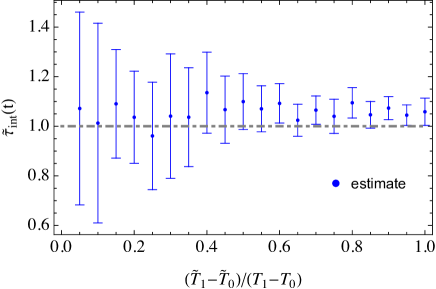
Figure 2: Results of $\tilde{\tau}_{\rm int}(t)$.

Figure 3 is the histogram of $p=(\tilde{T}_{1}-\tilde{T}_{0})/(T_{1}-T_{0})$, which is almost flat as required.

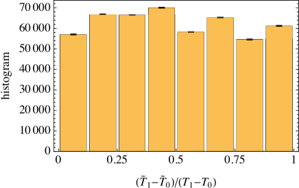
Figure 3: Histogram of $t$. The number of configurations in a bin is the average over 20 independent samples, each consisting of $N_{\rm conf}=5\times 10^{5}$. The function $W(t)$ is tuned such that the histogram becomes almost flat for these eight bins.

This is realized by tuning the functional form of $W(t)$ as in Ref. [23].

Figure 4 exhibits the scaling law (2.11) for three operators, $\mathcal{O}={\rm Re}\,(\bar{\psi}\psi A)$, $\mathcal{O}={\rm Re}\,(\psi^{\dagger}\psi A)$, and $\mathcal{O}={\rm Re}\,A$. We see that the scaling is satisfied for $\mathcal{O}={\rm Re}\,(\bar{\psi}\psi A)$ in the region $(\tilde{T}_{1}-\tilde{T}_{0})/(T_{1}-T_{0})\geq 0.35$, and for $\mathcal{O}={\rm Re}\,(\psi^{\dagger}\psi A)$ and $\mathcal{O}={\rm Re}\,A$ in the region $(\tilde{T}_{1}-\tilde{T}_{0})/(T_{1}-T_{0})\geq 0.20$. Deviations from the scaling at small $(\tilde{T}_{1}-\tilde{T}_{0})/(T_{1}-T_{0})$ should be due to $\tilde{\tau}_{\rm int}(\mathcal{O})=O(1)$ [see the comment below Eq. (2.8)].

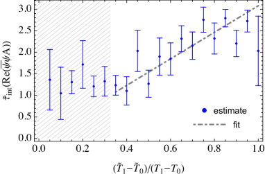
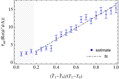
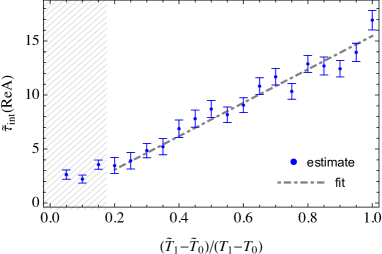
Figure 4: $\tilde{\tau}_{\rm int}(\mathcal{O})$ against $(\tilde{T}_{1}-\tilde{T}_{0})/(T_{1}-T_{0})$. Top left: $\mathcal{O}={\rm Re}\,(\bar{\psi}\psi A)$. Top right: $\mathcal{O}={\rm Re}\,(\psi^{\dagger}\psi A)$. Bottom: $\mathcal{O}={\rm Re}\,A$. Data points in the shaded region give $\tilde{\tau}_{\rm int}(\mathcal{O})=O(1)$ and thus are excluded from the linear fitting [see the comment below Eq. (2.8)].

We perform the $\chi^{2}$-fit to these data points with

$$\chi^{2}(\mathcal{O})\equiv\sum_{i=0}^{i_{\rm max}}\frac{[\tilde{\tau}^{(i)}_{\rm int}(\mathcal{O})-c\,(\tilde{T}_{1}-\tilde{T}_{0}^{(i)})/(T_{1}-T_{0})]^{2}}{[\delta\tilde{\tau}_{\rm int}^{(i)}(\mathcal{O})]^{2}},$$ (3.11)

where $\tilde{\tau}_{\rm int}^{(i)}(\mathcal{O})$ is the integrated autocorrelation time for the subsample with the interval $[\tilde{T}_{0},\tilde{T}_{1}]=[\tilde{T}_{0}^{(i)},T_{1}]$. The fit results are the following: For $\mathcal{O}={\rm Re}\,(\bar{\psi}\psi A)$ with $i_{\rm max}=13$, $c=3.1$ and $\chi^{2}/{\rm DOF}=1.0$. For $\mathcal{O}={\rm Re}\,(\psi^{\dagger}\psi A)$ with $i_{\rm max}=16$, $c=16.4$ and $\chi^{2}/{\rm DOF}=1.2$. For $\mathcal{O}={\rm Re}\,A$ with $i_{\rm max}=16$, $c=15.5$ and $\chi^{2}/{\rm DOF}=1.1$. These data support the scaling law (2.11).

We plot in Fig. 5 the values of $N_{\rm conf}^{\rm eff}(\mathcal{O};\tilde{T}_{0},\tilde{T}_{1})$ for various operators $\mathcal{O}$ [see Eq. (2.13)]. The statistical errors are estimated with the Jackknife method. We observe, as expected, that $N_{\rm conf}^{\rm eff}(\mathcal{O};\tilde{T}_{0},\tilde{T}_{1})$ takes almost the same values for each $\mathcal{O}$ in the range where we observe the scaling law.

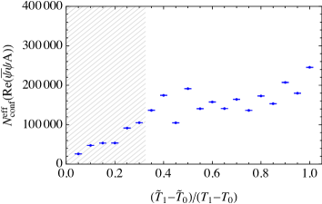
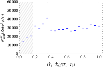
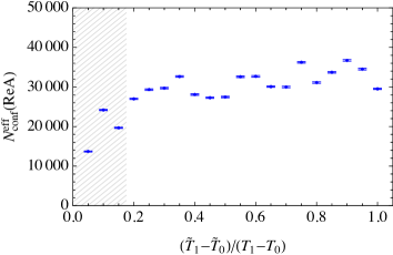
Figure 5: The values of $N_{\rm conf}^{\rm eff}(\mathcal{O};\tilde{T}_{0},\tilde{T}_{1})$ [see Eq. (2.13)]. Top left: $\mathcal{O}={\rm Re}\,(\bar{\psi}\psi A)$. Top right: $\mathcal{O}={\rm Re}\,(\psi^{\dagger}\psi A)$. Bottom: $\mathcal{O}={\rm Re}\,A$. The regions where the scaling law (2.11) is broken are shaded.

Finally, in Fig. 6 we plot the expectation values of the chiral condensate and the number density, together with their statistical errors.

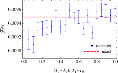
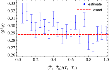
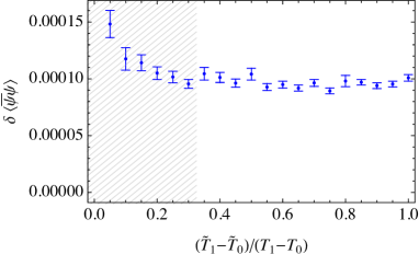
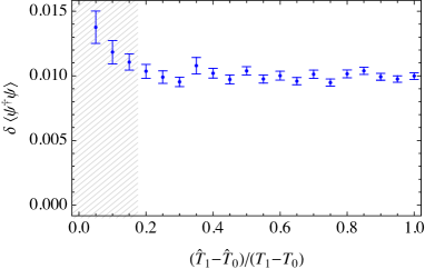
Figure 6: The estimate (top) and its statistical error (bottom) of the expectation value $\langle\mathcal{O}\rangle$ against $(\tilde{T}_{1}-\tilde{T}_{0})/(T_{1}-T_{0})$. Left: $\mathcal{O}=\bar{\psi}\psi$ (the chiral condensate). Right: $\mathcal{O}=\psi^{\dagger}\psi$ (the number density). The regions where the scaling law (2.11) is broken in the numerator and/or the denominator are shaded for the statistical errors.

The statistical errors are estimated with the Jackknife method with the bin sizes fixed to 500. We see that both the means and the statistical errors take almost constant values in a region where $(\tilde{T}_{1}-\tilde{T}_{0})/(T_{1}-T_{0})$ is not small. The deviation of the means should be attributed to the complex geometry at large flow times, which requires larger statistics and better control of systematic errors (such as those from numerical integrations of the flow equation and of the Hamilton equations accompanied by the projection from ${\mathbb{C}}^{N}$ to $\mathcal{R}$). The deviation of the statistical errors is due to the violation of the scaling law (2.11) for either of the numerator or the denominator (or both) in the ratio of the reweighted averages.

4 Summary and outlook

In this paper, we have established the statistical analysis method for the WV-HMC algorithm, whose major use is intended for the WV-TLTM [23]. We proved that, if consecutive configurations in the worldvolume are generated as a Markov chain with ergodicity and detailed balance, then the subset consisting of the configurations belonging to a subregion can also be regarded as a Markov chain with ergodicity and detailed balance intact. We particularly investigated the integrated autocorrelation times for the Markov chains in various subregions, and found that there is a linear relation between the probability to be in a subregion and the integrated autocorrelation time for the corresponding subsample. We numerically confirmed this scaling law for the Stephanov model.

Now with this statistical analysis method at hand, we can safely apply the WV-TLTM to large-scale simulations of the systems that have serious sign problems, such as finite density QCD, strongly correlated electron systems, frustrated spin systems, and the real-time dynamics of quantum fields. A study along this line is now in progress and will be reported elsewhere.

Appendix A Jackknife method for the integrated autocorrelation times

In this appendix, we give a Jackknife method to estimate the integrated autocorrelation times $\tau_{\rm int}(\mathcal{O})$.

Let $\{x_{j}\}$ $(j=1,\ldots,N_{\rm conf})$ be a set of consecutive configurations generated as a Markov chain. We estimate the expectation value $\langle\mathcal{O}\rangle$ by the sample average

$$\overline{\mathcal{O}}\equiv\frac{1}{N_{\rm conf}}\sum_{j=1}^{N_{\rm conf}}\mathcal{O}(x_{j}).$$ (A.1)

The estimator of the integrated autocorrelation time $\tau_{\rm int}(\mathcal{O})\equiv 1+2\sum_{k=1}^{\infty}C_{k}(\mathcal{O})/C_{0}(\mathcal{O})$ is given by

$$\bar{\tau}_{\rm int}(\mathcal{O};k_{\rm max})\equiv 1+2\sum_{k=1}^{k_{\rm max}}\frac{\overline{C}_{k}(\mathcal{O})}{\overline{C}_{0}(\mathcal{O})},$$ (A.2)

where $\overline{C}_{k}(\mathcal{O})$ is the estimator of the autocorrelation $C_{k}(\mathcal{O})\equiv\langle\mathcal{O}_{0}\,\mathcal{O}_{k}\rangle_{c}$. The summation is truncated at $k_{\rm max}$ to avoid summing up statistical fluctuations around zero (see, e.g., Refs. [27, 28]). The value of $k_{\rm max}$ should not be set very large compared to $\tau_{\rm int}(\mathcal{O})$, otherwise contributions from statistical fluctuations around zero may dominate the error. There has been known an explicit formula for the statistical error $\delta\tau_{\rm int}(\mathcal{O})$ when $1\ll k_{\rm max}\ll N_{\rm conf}$ (more precisely, as $N_{\rm conf}\to\infty$, $k_{\rm max}\to\infty$ and $k_{\rm max}/N_{\rm conf}\to 0$) [26] (see also Refs. [27, 28]), but this may not be applicable to the case when $\tau_{\rm int}(\mathcal{O})=O(1)$, for which the condition $k_{\rm max}\gg 1$ cannot be met. Therefore, in this paper we adopt the Jackknife method for the estimation of $\delta\tau_{\rm int}(\mathcal{O})$.

In order to apply a resampling method of Jackknife, we introduce a sample of multidimensional observables $\{X_{r}=(X_{r,k}^{\mathcal{O}\mathcal{O}},X_{r}^{\mathcal{O}})\}$ ($r=1,\ldots,N_{\rm conf}-k_{\rm max}$) with

$$X_{r,k}^{\mathcal{O}\mathcal{O}}\equiv\frac{1}{k_{\rm max}-k+1}\sum_{i=0}^{k_{\rm max}-k}\mathcal{O}(x_{r+i})\mathcal{O}(x_{r+k+i})\quad(k=0,\ldots,k_{\rm max}),$$ (A.3)

$$X_{r}^{\mathcal{O}}\equiv\frac{1}{k_{\rm max}+1}\sum_{i=0}^{k_{\rm max}}\mathcal{O}(x_{r+i}).$$ (A.4)

Since $\langle X_{r,k}^{\mathcal{O}\mathcal{O}}\rangle=\langle\mathcal{O}(x_{0})\,\mathcal{O}(x_{k})\rangle$ and $\langle X_{r}^{\mathcal{O}}\rangle=\langle\mathcal{O}(x)\rangle$, the autocorrelations $C_{k}(\mathcal{O})=\langle\mathcal{O}(x_{0})\mathcal{O}(x_{k})\rangle_{c}$ can be estimated by

$$\overline{C}^{(X)}_{k}(\mathcal{O})\equiv\frac{1}{N_{\rm conf}-k_{\rm max}}\sum_{r=1}^{N_{\rm conf}-k_{\rm max}}X_{r,k}^{\mathcal{O}\mathcal{O}}-\bigg{(}\frac{1}{N_{\rm conf}-k_{\rm max}}\sum_{r=1}^{N_{\rm conf}-k_{\rm max}}X_{r}^{\mathcal{O}}\bigg{)}^{2}.$$ (A.5)

Since $\tau_{\rm int}(\mathcal{O})$ is a function of $C_{k}(\mathcal{O})$, it can be estimated with $\overline{C}^{(X)}_{k}(\mathcal{O})$ as

$$\tau_{\rm int}(\mathcal{O})\approx 1+2\sum_{k=1}^{k_{\rm max}}\frac{\overline{C}^{(X)}_{k}(\mathcal{O})}{\overline{C}^{(X)}_{0}(\mathcal{O})}.$$ (A.6)

The statistical error $\delta\tau_{\rm int}(\mathcal{O})$ can then be estimated with the standard Jackknife method.

References

- [1] G. Aarts, Introductory lectures on lattice QCD at nonzero baryon number. J. Phys. Conf. Ser. 706, no. 2, 022004 (2016) [arXiv:1512.05145 [hep-lat]].
- [2] L. Pollet, Recent developments in Quantum Monte-Carlo simulations with applications for cold gases, Rep. Prog. Phys. 75, 094501 (2012) [arXiv:1206.0781 [cond-mat.quant-gas]].
- [3] G. Parisi, “On complex probabilities,” Phys. Lett. B 131, 393 (1983).
- [4] J.R. Klauder, “Coherent State Langevin Equations for Canonical Quantum Systems With Applications to the Quantized Hall Effect,” Phys. Rev. A 29, 2036 (1984).
- [5] G. Aarts, F. A. James, E. Seiler and I. O. Stamatescu, “Adaptive stepsize and instabilities in complex Langevin dynamics,” Phys. Lett. B 687, 154-159 (2010) [arXiv:0912.0617 [hep-lat]].
- [6] J. Nishimura and S. Shimasaki, “New Insights into the Problem with a Singular Drift Term in the Complex Langevin Method,” Phys. Rev. D 92, no.1, 011501 (2015) [arXiv:1504.08359 [hep-lat]].
- [7] Y. Mori, K. Kashiwa and A. Ohnishi, “Toward solving the sign problem with path optimization method,” Phys. Rev. D 96, no.11, 111501 (2017) [arXiv:1705.05605 [hep-lat]].
- [8] Y. Mori, K. Kashiwa and A. Ohnishi, “Application of a neural network to the sign problem via the path optimization method,” PTEP 2018, no.2, 023B04 (2018) [arXiv:1709.03208 [hep-lat]].
- [9] A. Alexandru, P. F. Bedaque, H. Lamm and S. Lawrence, “Finite-Density Monte Carlo Calculations on Sign-Optimized Manifolds,” Phys. Rev. D 97, no.9, 094510 (2018) [arXiv:1804.00697 [hep-lat]].
- [10] F. Bursa and M. Kroyter, “A simple approach towards the sign problem using path optimisation,” JHEP 12, 054 (2018) [arXiv:1805.04941 [hep-lat]].
- [11] E. Witten, “Analytic continuation of Chern-Simons theory,” AMS/IP Stud. Adv. Math. 50, 347-446 (2011) [arXiv:1001.2933 [hep-th]].
- [12] M. Cristoforetti, F. Di Renzo and L. Scorzato, “New approach to the sign problem in quantum field theories: High density QCD on a Lefschetz thimble,” Phys. Rev. D 86, 074506 (2012) [arXiv:1205.3996 [hep-lat]].
- [13] M. Cristoforetti, F. Di Renzo, A. Mukherjee and L. Scorzato, “Monte Carlo simulations on the Lefschetz thimble: Taming the sign problem,” Phys. Rev. D 88, no. 5, 051501(R) (2013) [arXiv:1303.7204 [hep-lat]].
- [14] H. Fujii, D. Honda, M. Kato, Y. Kikukawa, S. Komatsu and T. Sano, “Hybrid Monte Carlo on Lefschetz thimbles - A study of the residual sign problem,” JHEP 1310, 147 (2013) [arXiv:1309.4371 [hep-lat]].
- [15] H. Fujii, S. Kamata and Y. Kikukawa, “Lefschetz thimble structure in one-dimensional lattice Thirring model at finite density,” JHEP 11, 078 (2015) [erratum: JHEP 02, 036 (2016)] [arXiv:1509.08176 [hep-lat]].
- [16] H. Fujii, S. Kamata and Y. Kikukawa, “Monte Carlo study of Lefschetz thimble structure in one-dimensional Thirring model at finite density,” JHEP 12, 125 (2015) [erratum: JHEP 09, 172 (2016)] [arXiv:1509.09141 [hep-lat]].
- [17] A. Alexandru, G. Başar and P. Bedaque, “Monte Carlo algorithm for simulating fermions on Lefschetz thimbles,” Phys. Rev. D 93, no. 1, 014504 (2016) [arXiv:1510.03258 [hep-lat]].
- [18] A. Alexandru, G. Başar, P. F. Bedaque, G. W. Ridgway and N. C. Warrington, “Sign problem and Monte Carlo calculations beyond Lefschetz thimbles,” JHEP 1605, 053 (2016) [arXiv:1512.08764 [hep-lat]].
- [19] M. Fukuma and N. Umeda, “Parallel tempering algorithm for integration over Lefschetz thimbles,” PTEP 2017, no. 7, 073B01 (2017) [arXiv:1703.00861 [hep-lat]].
- [20] A. Alexandru, G. Başar, P. F. Bedaque and N. C. Warrington, “Tempered transitions between thimbles,” Phys. Rev. D 96, no. 3, 034513 (2017) [arXiv:1703.02414 [hep-lat]].
- [21] M. Fukuma, N. Matsumoto and N. Umeda, “Applying the tempered Lefschetz thimble method to the Hubbard model away from half filling,” Phys. Rev. D 100, no. 11, 114510 (2019) [arXiv:1906.04243 [cond-mat.str-el]].
- [22] M. Fukuma, N. Matsumoto and N. Umeda, “Implementation of the HMC algorithm on the tempered Lefschetz thimble method,” [arXiv:1912.13303 [hep-lat]].
- [23] M. Fukuma and N. Matsumoto, “Worldvolume approach to the tempered Lefschetz thimble method,” PTEP 2021, no.2, 023B08 (2021) [arXiv:2012.08468 [hep-lat]].
- [24] M. A. Stephanov, “Random matrix model of QCD at finite density and the nature of the quenched limit,” Phys. Rev. Lett. 76, 4472 (1996) [hep-lat/9604003].
- [25] M. A. Halasz, A. D. Jackson, R. E. Shrock, M. A. Stephanov and J. J. M. Verbaarschot, “On the phase diagram of QCD,” Phys. Rev. D 58, 096007 (1998) [hep-ph/9804290].
- [26] N. Madras and A. D. Sokal, “The pivot algorithm: A highly efficient Monte Carlo method for self-avoiding walk,” J. Stat. Phys. 50, 109 (1988).
- [27] U. Grenander and M. Rosenblatt, “Statistical Spectral Analysis of Time Series Arising from Stationary Stochastic Processes,” Ann. Math. Statist. 24 (4) 537 - 558 (1953).
- [28] M. B. Priestley, “Spectral analysis and time series,” Academic Press, London (1981).