Correlation scenarios and correlation stress testing

Abstract

We develop a general approach for stress testing correlations of financial asset portfolios. The correlation matrix of asset returns is specified in a parametric form, where correlations are represented as a function of risk factors, such as country and industry factors. A sparse factor structure linking assets and risk factors is built using Bayesian variable selection methods. Regular calibration yields a joint distribution of economically meaningful stress scenarios of the factors. As such, the method also lends itself as a reverse stress testing framework: using the Mahalanobis distance or highest density regions (HDR) on the joint risk factor distribution allows to infer worst-case correlation scenarios. We give examples of stress tests on a large portfolio of European and North American stocks.

Keywords: Correlation stress testing, reverse stress testing, factor selection, scenario selection, Bayesian variable selection, market risk management

JEL classification: G11, G32

1 Introduction

Correlation is one of the most important, if not the most important risk factor in finance, driving everything from naïve diversification to the effectiveness of hedges. It is well-established that correlations fluctuate over time and may be strongly affected by specific events (Karolyi and Stulz, 1996; Longin and Solnik, 2001; Ang and Bekaert, 2002; Wied et al., 2012; Pu and Zhao, 2012; Adams et al., 2017). Changes in correlation may lead to potentially unexpected or unquantified losses, see e.g. LTCM (Jorion, 2000), Amaranth Advisors (Chincarini, 2007), JPMorgan’s “London Whale” (Packham and Woebbeking, 2019). Regulators have since called for a better correlation risk management. However, a unified and generally accepted correlation risk management framework does not yet exist.

Building on the work of Packham and Woebbeking (2019), this article develops a universal framework for building realistic correlation scenarios, correlation stress testing and reverse stress testing. The novelty of this approach is the link between correlations and observable risk factors. “Classical” stress testing determines the impact on a financial position as a consequence of changes in risk factors, see e.g. (EBA, 2021). Here, we consider the impact on asset correlations of a risk factor scenario. With this framework, one can challenge diversification benefits based on economic scenarios. Likewise, one can assess the effectiveness and risks of hedges based on economic scenarios. In particular, correlation stress tests produce extreme, yet plausible correlation scenarios from economically relevant risk factors. Our method therefore addresses: first, the selection of appropriate correlation risk factors for a given portfolio; second, the parameterization of large correlation matrices and their mapping into risk measures; third, the identification of critical scenarios through reverse stress testing. The method is particularly relevant for supervisors who “are considering the ways in which stress tests can be integrated best into the regulatory framework” (Pliszka, 2021). Reverse stress testing complements other stress testing methods, such as stressed value-at-risk, introduced in the Basel 2.5 framework (BIS, 2011). Stressed VaR determines portfolio risk using the parameters of a time period considered as stressful. Reverse stress testing, on the other hand, determines the risk factor configuration that is both stressful and plausible for a given portfolio.

Contrary to extremely prudent scenarios where diversification effects are ignored, we are particularly interested in establishing a link between risk factors and assessing the plausibility of scenarios. It is this link that enables reverse stress testing, i.e., the identification of critical risk factor scenarios, which, from the point of view of a practitioner, may see as the most valuable aspect of stress testing.

A widespread method in financial risk management and in asset management is to capture correlations through factor models, see e.g. (McNeil et al., 2005, Section 3.4). A common choice for the factors are industries and geographic regions. In this article, correlations are modelled by linking each asset to a subset out of the set of factors. Asset correlations are specified in a functional form, where the correlation between any two assets is determined by the shared, resp. unshared links. The degree by which shared or unshared links affect correlations is obtained by calibrating “weight” parameters to empirical correlations. Scenarios are generated by varying these parameters.

Given the history of calibrated parameters, the method lends itself to reverse stress testing as it is capable of identifying the factor structure of worst case scenarios. More specifically, given the mapping of correlation risk factors to a risk measure, one can find the global maximum of the risk measure and infer the corresponding risk factor scenario. As each parameter represents an economically relevant correlation risk factor, it is therefore possible to identify critical portfolio structures (“smoking guns”) that might require particular attention from a risk management perspective.

Plausibility, or lag thereof, is a common problem for scenarios that are generated through reverse stress testing. This article addresses plausibility by assigning a joint probability distribution to the correlation parameters, which in turn allows to quantify the plausibility of correlation scenarios. In this article, the constraint is specified via the Mahalanobis distance and highest density regions (HDR), both of which can be thought of generalising the concept of a quantile to a multivariate setting, as will be explained below.

Assigning the appropriate correlation risk factors to an asset is a delicate exercise: ignoring relevant risk factors might lead to undetected correlation risk, while selecting an excessive amount of risk factors potentially renders the economic interpretation meaningless, as the impact of specific risk drivers becomes indistinguishable across assets. A good factor selection mechanism should therefore focus on a sparse selection of relevant factors for each asset. In addition, since typically some persistent information about the relationships between assets and factors is available (such as the country of the headquarter and the main industry), the factor selection method should offer the ability to incorporate prior knowledge. Bayesian variable selection methods support both of these requirements by allowing to specify prior information as well a giving control over the number of factors selected.

The framework developed here can be implemented for any financial application that bears correlation risk, such as asset allocation or hedging. As an example, we apply the factor-model approach to a large and well-diversified equity portfolio. For this particular portfolio, geographic regions and industries serve as correlation risk factors.

A further application where correlation scenario and stress testing can reveal inherent risks is the practice of so-called “portfolio margining” in initial margin calculations of clearing houses. Here, netting of offsetting positions reduces the margin requirement. However, if positions hedging each other are not perfect substitutes, but only highly correlated, then significant de-correlation could lead to substantial margin calls, thereby increasing counterparty risk at a systematic level.

The literature on the role of correlation and dependence in finance is vast, but interestingly the literature on establishing correlation stress tests is comparably scarce. It is well established that correlations are not constant over time and may be strongly affected by specific events (Longin and Solnik, 2001; Wied et al., 2012; Pu and Zhao, 2012). Adams et al. (2017) observe that correlations vary over time and, in addition, experience level shifts and structural breaks that occur in response to economic or financial shocks. The regime switching behaviour of financial asset correlations, especially in times of crisis, is confirmed and at the heart of several studies, including Sandoval Jr. and Franca (2012); Buccheri et al. (2013); Papenbrock and Schwendner (2015). Krishnan et al. (2009) and Mueller et al. (2017) provide empirical evidence that investors demand a correlation risk premium, which is related to the uncertainty about future correlation changes. Buraschi et al. (2010) develop a framework for inter-temporal portfolio choice that includes hedging components against correlation risk. Tumminello et al. (2010); Keskin et al. (2011) analyse the topology of correlation matrices as networks or hierarchical trees, providing insights on the structure, taxonomy and hierarchy of financial asset correlations. This last strand of the literature is probably closest to our framework in the sense that it provides an interpretation of the factors driving correlation changes.

Packham and Woebbeking (2019) introduce a correlation stress testing methodology tailored to the case of the so-called “London Whale”, a USD 6.2 billion loss on a credit derivatives portfolio at JPMorgan. The loss was partly due to the de-correlation of positions that were supposed to act as hedges for each other. Correlation stress testing would have revealed this risk early on and might therefore have led to a more prudent assessment and de-leveraging of the position. The factors in the “London Whale” case were tailored to match characteristics of the credit derivatives, such as their maturity, credit quality (investment grade versus high yield) and geographic origin (CDX in the US, iTraxx in Europe).

The prominent role of correlation in financial portfolios has led regulatory agencies to call for risk model stress tests that account for “significant shifts in correlations” (BCBS, 2006, p. 207 ff.). However, there is little literature on parametric correlation modelling, an exception being parametric functions for correlation and volatility in interest rate modelling (e.g. LIBOR market model), see Rebonato (2002); Brigo (2002); Schoenmakers and Coffey (2003). Another strand of the literature on correlation stress testing deals with the question of ensuring positive semi-definiteness of the matrix, see Higham (2002); Qi and Sun (2010); Ng et al. (2014).

The selection of plausible scenarios poses a challenge in the development of stress testing methods in general. The use of historical or hypothetical scenarios is problematic, as the probability and thus the plausibility of a scenario is unknown and relevant scenarios might be neglected. In an extensive study, Alexander and Sheedy (2008) compare various well-known models in their ability to conduct meaningful stress tests. Glasserman et al. (2015) develop an empirical likelihood approach for the selection of stress scenarios, with a focus on reverse stress testing. Kopeliovich et al. (2015) present a reverse stress testing method to determine scenarios that lead to a specified loss level. Breuer et al. (2009) and Flood and Korenko (2015) use the Mahalanobis distances to select scenarios from a multivariate distribution of risk factors.

Breuer and Csiszár (2013) extend these approaches and consider various application scenarios, amongst them stressed default correlations, which refer to the correlations of Bernoulli variables denoting the default or survival of loans or obligors. Studer (1999) considers correlation breakdowns by identifying the worst-case correlation scenario in a constrained region of P&L scenarios. However, solving the problem turns out to be computationally intractable. Also, the likelihood or plausibility of such a correlation scenario is not known. The difference in our setting is that we model correlation itself in a parametric way and – imposing a risk factor distribution calibrated from historical data – find the risk-factor scenario that produces the worst loss within a given plausibility region.

In summary, we contribute to the literature by proposing a flexible correlation stress testing framework that is capable of adapting to different requirements and settings. A central feature of our method is the Bayesian selection of correlation risk factors. Choosing the “right” factors is a timely and relevant exercise, especially from a regulatory perspective. Furthermore, we explore how reverse stress testing can help to construct and understand extreme yet plausible risk factor scenarios. This article tests the method on a large equity portfolio; however, the method would easily adopt to any other financial portfolio.

The article is structured as follows: Section 2 lays out the factor model for correlation stress testing. Section 3 introduces the Bayesian correlation factor selection mechanism. Section 4 applies the stress testing framework to a large stock portfolio; and Section 5 concludes.

2 Correlation stress testing methodology

This section presents the correlation stress testing framework. First, we define a factor model structure on correlations, which establishes a correlation matrix under stress. Second, we infer the impact of the stressed correlations by calculating value-at-risk with the modified correlation matrix. Finally, by imposing a probability distribution on the factors driving correlation, we determine plausible worst-case correlation stress scenarios. The last step is commonly known as reverse stress testing.

2.1 Factor model

An economically meaningful correlation stress testing framework requires linking correlations with risk factors, such as economic variables or financial market indicators. In the context of portfolio allocation or risk management, the factors could represent industries and countries. While Packham and Woebbeking (2019) applied correlation stress testing in a very specific context, this article aims to develop a generic and flexible correlation stress testing framework, intended to work in different contexts and for different applications.

Consider a portfolio of $p$ assets and assume that there are $d$ risk factors. Each asset is associated with a number of these risk factors. We will introduce details on how factors are assigned in Section 3; it should be noted, however, that for a stress test to be meaningful, the number of factors associated with an asset needs to be sufficiently small.

The association of asset $i\in\{1,\ldots,p\}$ with factor $k\in\{1,\ldots,d\}$ is denoted by the indicator variable $\mathbf{1}_{\{k,i\}}$. The correlation of asset returns $i$ and $j$ is modelled as

$$c_{ij}=\text{tanh}\Big{(}\eta+\underbrace{\sum_{k=1}^{d}\lambda_{k}|\mathbf{1}_{\{k,i\}}-\mathbf{1}_{\{k,j\}}|}_{\text{``inter''-correlations}}+\underbrace{\sum_{k=1}^{d}\nu_{k}\mathbf{1}_{\{k,i\}}\mathbf{1}_{\{k,j\}}}_{\text{``intra''-correlations}}\Big{)},$$ (1)

with coefficients $\eta,\lambda_{1},\ldots,\lambda_{d},\nu_{1},\ldots,\nu_{d}\in{\mathbb{R}}$ and $\text{tanh}:{\mathbb{R}}\mapsto[-1,1]$ the tangens hyperbolicus. Aside from conveniently mapping to $[-1,1]$ and being monotone increasing, the main motivation for choosing the function tanh is its use in inferential statistics on sample correlation coefficients. The following summation formula serves as useful a approximation for the interpretation of individual coefficients, especially if the coefficients are close to zero:

$$\tanh(x+y)=\frac{\tanh x+\tanh y}{1+\tanh x\tanh y}\approx\tanh x+\tanh y.$$ (2)

The constant $\eta$ can be thought of as a “base” correlation. The coefficients $\lambda_{1},\ldots,\lambda_{d}$ model “inter-factor” correlations: the higher $\lambda_{k}$, the higher the correlation impact if exactly one of the two assets is associated with the $k$-th factor (in which case $|\mathbf{1}_{\{k,i\}}-\mathbf{1}_{\{k,j\}}|=1$). Similarly, $\nu_{1},\ldots,\nu_{d}$ express “intra-factor” correlation: the higher $\nu_{k}$, the higher the correlation between assets jointly exposed to factor $k$ (since in this case $\mathbf{1}_{\{k,i\}}\mathbf{1}_{\{k,j\}}=1$). The concept of “inter”- and “intra”-correlations is found in the context of credit risk in e.g. (Düllmann et al., 2008).

Given a sample correlation matrix at one point in time, the coefficients $\eta,\lambda_{1},\ldots,\lambda_{d},\nu_{1},\ldots,\nu_{d}$ can be determined e.g. by ordinary least squares on $\text{arctanh}(c_{ij})$, the inverse of tanh. Simple correlation scenarios such as “the correlation between assets exposed to factor $k$ and assets not exposed to factor $k$ increases” is then implemented by increasing $\lambda_{k}$. Likewise, a scenario such as “the correlation of firms exposed to factor $k$ increases” is implemented by increasing $\nu_{k}$. With time series of historical data, the coefficients can be calibrated on a regular basis, from which resonable scenarios can be determined.

The matrix defined by Equation (1) is not guaranteed to be positive semidefinite and thus may need to be further transformed to yield a valid correlation matrix. Converting a non-positive-semidefinite matrix $\tilde{C}\in\mathbb{R}^{n\times n}$ into a positive-semidefinite matrix can be approached as a matrix nearness problem, with nearness expressed by a suitable norm, such as the Frobenius norm (sum of absolute difference of all matrix entries). Higham (2002) provides an algorithm that finds the correlation matrix satisfying $\min\{||\tilde{C}-C||:C\text{ is a correlation matrix}\}$ by exploiting the spectral properties of $\tilde{C}$. It may also be possible that a correlation matrix fails to be positive semidefinite due to computational precision, in which case the eigenvalues of the matrix are just slightly below zero. In this case it can be sufficient to transform the matrix as $C=(1-\epsilon)\tilde{C}+\epsilon I$, where $I$ is the identity matrix and $\epsilon$ is a small constant.

2.2 Stress testing

With a portfolio’s value being just the sum the constituents’ values, a ceteris paribus shift in correlation has no instantaneous effect on the value. Therefore, to reveal the impact of a correlation stress test requires calculating portfolio risk measures. In the simplest setting, portfolio risk is measured by value-at-risk (VaR) in a variance-covariance approach, i.e.,

$$\text{VaR}_{\alpha}=-{\rm N}_{1-\alpha}\cdot V_{0}\cdot\left(\mathbf{w}^{\intercal}\,\boldsymbol{\Sigma}\,\mathbf{w}\right)^{1/2},$$ (3)

where ${\rm N}_{1-\alpha}$ denotes the $(1-\alpha)$-quantile of the standard normal distribution, $V_{0}$ denotes the current position value, $\mathbf{w}$ is the vector of portfolio weights and $\boldsymbol{\Sigma}$ denotes the covariance matrix of the portfolio returns. In this setting we assume that the expected return is zero, which is a common and reasonable assumption for short time horizons.

The normal distribution assumption can easily be generalised, e.g. to a Student $t$-distribution. The $t$-VaR is discussed in Packham and Woebbeking (2019), together with the possibility to jointly apply correlation and volatility stress scenarios. In fact, any model or method that takes a correlation matrix as an input is suitable for the correlation stress testing approach.

2.3 Reverse stress testing

When stress testing, aside from understanding the impact of given scenarios, one is also interested in the opposite question: What is the worst scenario amongst all scenarios that occur within some pre-given range? In a univariate setting, one would select a quantile of the risk factor distribution – this is the principal idea underlying value-at-risk. Different extensions of quantiles to a multivariate setting exist, for example the Mahalanobis distance (Mahalanobis, 1936), highest density regions (HDR) (Hyndman, 1996) or concepts based on norms, see e.g. (Serfling, 2002).

The Mahalanobis distance of a vector $\mathbf{X}\in{\mathbb{R}}^{n}$ with expectation $\mathbf{\mu}\in{\mathbb{R}}^{n}$ and covariance $\boldsymbol{\Sigma}\in{\mathbb{R}}^{n}\times{\mathbb{R}}^{n}n$ is defined as $D(\mathbf{x},\mathbf{\mu},\boldsymbol{\Sigma})=(\mathbf{x}-\mathbf{\mu})^{\intercal}\boldsymbol{\Sigma}^{-1}(\mathbf{x}-\mathbf{\mu})$, see e.g. (Mahalanobis, 1936; Kent et al., 1979; McNeil et al., 2005). The Mahalanobis distance is an appropriate measure for reverse stress testing if the underlying distribution is elliptic or at least symmetric. Moreover, if $\mathbf{X}$ is normally distributed, then $D^{2}(\mathbf{X})\sim\chi^{2}(n)$, where $n$ is the length of $\mathbf{X}$, which greatly simplifies identifying if scenarios lie within a range specified by a probability.

The highest-density region (HDR) (Hyndman, 1996) generalises the idea of the Mahalanobis distance to arbitrary probability distributions. It is defined as the region with probability $1-\alpha$ that has the smallest possible volume in the sample space; equivalently, every point inside the region should have probability density at least as large as every point outside of the region. Formally, if $f(\mathbf{x})$ is the density of $\mathbf{X}$, then the $(1-q)$–HDR is the subset $R(f_{q})$ of the sample space such that $R(f_{q})=\{x:f(x)\geq f_{q}\}$, where $f_{q}$ is the largest constant such that ${\bf P}(\mathbf{X}\in R(f_{q}))\geq 1-q$.

A straightforward way to calculate the HDR is via Monte Carlo simulation, see Hyndman (1996). Note that ${\bf P}(f(\mathbf{X})\geq f_{q})=1-q$; in other words, $f_{q}$ is the $q$-quantile of $f(\mathbf{X})$. Given an iid sample of observations, $f_{q}$ can be estimated from the sample, and all samples in the HDR are easily identified by having a density value greater than $f_{q}$. If the sample size is large enough, then a reduction of the estimator’s variance is achieved by a variant of Latin Hypercube Sampling (LHS) targeted at dependent random vectors (Packham and Schmidt, 2010).

In order to allow for skewness and more variation in tail heaviness than a normal distribution, we calibrate the time series of coefficients $\boldsymbol{\beta}=(\eta,\lambda_{1},\ldots,\lambda_{d},\eta_{1},\ldots,\eta_{d})^{\intercal}$ to a multivariate normal inverse Gaussian (NIG) distribution (see Appendix A) and infer reverse stress test scenarios as the worst scenarios within the HDR at a given level $\alpha$, i.e.,

$$\boldsymbol{\beta}^{\ast}=\operatornamewithlimits{argmax}_{\{\boldsymbol{\beta}\in R(f_{q})\}}\text{VaR}_{\alpha}(\boldsymbol{\beta}),$$ (4)

where $\text{VaR}_{\alpha}$ is given by Equation (3) with correlation matrix imposed by $\boldsymbol{\beta}$. From Equation (3), it is obvious that maximising $\text{VaR}_{\alpha}$ does not depend on $\alpha$ and is equivalent to maximising the variance. A trivial consequence is that $\boldsymbol{\beta}^{\ast}$ also maximises expected shortfall $\displaystyle\text{ES}_{\alpha}=\frac{1}{1-\alpha}\int_{\alpha}^{1}\text{VaR}_{u}\,{\rm d}u$.

3 Factor selection

As mentioned in the introduction, Packham and Woebbeking (2019) demonstrate the correlation stress testing methodology tailored to the case of the so-called “London Whale”, where the factors were manually chosen to match characteristics of the underlying credit derivatives portfolio, such as their maturity, credit quality (investment grade versus high yield) and geographic origin (CDX in the US, iTraxx in Europe).

In general, the choice of factors will depend on the type of correlation stress test to be conducted, and the assignment of relevant factors to assets may not be as straightforward as in the “London Whale” case. In a standard credit risk or asset allocation setting, one could choose industries and geographic locations as factors. While it is straightforward to assign one industry and one geographic location to a company, this may fail capture the dependence on further relevant industries and geographic locations of internationally operating firms.

We employ Bayesian variable selection (BVS) methods using both the prior knowledge of the main industry and headquarter location of a firm and allowing to select further factors, while controlling the expected number of factors. This gives a stable assignment of factors to assets to be used in (1).

To this end we impose a linear factor structure on asset returns. In a (linear) factor model (see e.g. Chapter 6 of (McNeil et al., 2015)), the return vector of $p$ firms, $\bm{r}=(r_{1},\ldots,r_{p})^{T}$, is represented as

$$r_{i}=\alpha_{i}+\beta_{i1}x_{1}+\beta_{i2}x_{2}+\cdots+\beta_{id}x_{d}+\varepsilon_{i},\qquad i=1,\ldots,p,$$

where $x_{1},\ldots,x_{d}$ are the common factors, $\beta_{i1},\beta_{i2},\ldots,\beta_{id}$ are the factor loadings and $\bm{\varepsilon}=(\varepsilon_{1},\ldots,\varepsilon_{p})^{T}$ are the idiosyncratic error terms, assumed to be uncorrelated and with mean $0$. Contrary to an OLS estimator, which typically assigns non-zero factor loadings to all factors, methods such as Lasso (e.g. Hastie et al. (2009)) select a (small) subset of factors by assigning both zero and non-zero factor loadings. If identical priors for all factors are used, then Lasso could be employed instead of a BVS method (see (Fahrmeir et al., 2013, Section 4.4.2) for the connection of Lasso and BVS). However, given that prior knowledge about some factors (e.g. the company VW is an automotive company headquartered in Germany) is available, a BVS method with non-identical priors is preferred.

Below we outline Bayesian model selection, the method used in this article. A further popular BVS method, BVS with spike and slab priors, is developed in (George and McCulloch, 1997).

For every firm $i$, we estimate the posterior inclusion probability (PIP) of each factor $k$ and set $\mathbf{1}_{k,i}=1$ if the PIP is greater than $1/2$. This is the so-called median probability model. Barbieri and Berger (2004) show that the median probability model is often optimal in terms of prediction. In our example, prior is initially set to force inclusion of a firm’s headquarter’s country and its primary industry, all other prior inclusion probabilities are set to include six factors on average. As the PIP’s are recalibrated periodically, the current PIP’s are chosen as the new prior inclusion probabilities. This provides a greater stability of the parameters over time.

3.1 Bayesian linear model

We consider the linear model

$$\bm{y}=\bm{X}\bm{\beta}+\bm{\varepsilon}.$$

In the Bayesian setting – see Section 3.5 (Fahrmeir et al., 2013) – we assume that

$$\bm{y}|\bm{\beta},\sigma^{2}\sim{\rm N}(\bm{X}\bm{\beta},\sigma^{2}\bm{I}),$$

with $\bm{\beta}$ and $\sigma^{2}$ stochastic.

A conjugate prior, i.e., where the prior and the posterior distributions are from the same distribution family, is

$$\bm{\beta}|\sigma^{2} \sim{\rm N}(\bm{m},\sigma^{2}\bm{M})$$

$$\sigma^{2} \sim\text{IG}(a,b),$$

where $\text{IG}(a,b)$ denotes the inverse gamma distribution with parameters $a,b$. An equivalent formulation is that the pair $(\bm{\beta},\sigma^{2})$ follows an normal inverse gamma distribution

$$(\bm{\beta},\sigma^{2})\sim\text{N-}\Gamma^{-1}(\bm{m},\bm{M},a,b).$$

The posterior distribution is given as (see e.g. Fahrmeir et al. (2013))

$$(\bm{\beta},\sigma^{2})|\bm{y} \sim\text{N-}\Gamma^{-1}(\tilde{\bm{m}},\tilde{\bm{M}},\tilde{a},\tilde{b}),$$

where

$$\tilde{\bm{M}} =\left(\bm{X}^{\prime}\bm{X}+\bm{M}^{-1}\right)^{-1}$$

$$\tilde{\bm{m}} =\tilde{\bm{M}}\left(\bm{M}^{-1}\bm{m}+\bm{X}^{\prime}\bm{y}\right)$$

$$\tilde{a} =a+\frac{n}{2}$$

$$\tilde{b} =b+\frac{1}{2}\left(\bm{y}^{\prime}\bm{y}+\bm{m}^{\prime}\bm{M}^{-1}\bm{m}-\tilde{\bm{m}}^{\prime}\tilde{\bm{M}}^{-1}\tilde{\bm{m}}\right).$$

3.2 Bayesian model comparison and selection

This method for variable selection considers candidate models $M_{i}$, $i=1,\ldots,m$. In the linear setting, each model $M_{i}$ includes a specific set of independent variables and excludes the other variables. For the posterior model probability we have

$$p(M_{i}|\bm{y})\propto p(\bm{y}|M_{i})p(M_{i}),$$

with $p(\bm{y}|M_{i})$ the so-called marginal likelihood. Define indicator variables $\gamma_{1},\ldots,\gamma_{d}$, with $\gamma_{k}=\mathbf{1}_{\{\beta_{k}\not=0\}}$,i.e., if $\gamma_{k}=1$, then the $x_{k}$ is included in the model. A prior model is then

$$p(M_{i})=\prod_{k=1}^{d}w_{k}^{\gamma_{k}}(1-w_{k})^{1-\gamma_{k}},$$

where $w_{k}\in[0,1]$, $k=1,\ldots,d$. If $w_{k}=1/2$, then $p(M_{i}|\bm{y})\propto p(\bm{y}|M_{i})$.

In our setting we set $w_{k}=1$ initially for the industry and location that is hard-coded for a firm (this data is available on Bloomberg). All other weights $w_{k}$ are set to $\theta={\mathbb{E}}[S]/d$, where $S$ is the (unknown) model size. Under the assumption that $S$ follows a binomial distribution $B(d,\theta)$, ${\mathbb{E}}(S)=\theta\cdot d$, so $\theta$ is chosen to attain a target expected model size.

The marginal likelihood can be calculated from the poster density for model $M_{i}$,

$$p(\bm{\beta},\sigma^{2}|\bm{y},M_{i})=\frac{p(\bm{y}|\bm{\beta},\sigma^{2},M_{i})p(\bm{\beta},\sigma^{2}|M_{i})}{p(\bm{y}|M_{i})},$$

by re-arranging to

$$p(\bm{y}|M_{i})=\frac{p(\bm{y}|\bm{\beta},\sigma^{2},M_{i})p(\bm{\beta},\sigma^{2}|M_{i})}{p(\bm{\beta},\sigma^{2}|\bm{y},M_{i})}.$$

This can be calculated analytically or by Markov Chain Monte Carlo methods (MCMC) if the number of models, $2^{d}$, is large. The posterior probability of $\gamma_{k}$ across all models is given by the posterior inclusion probability (PIP),

$${\bf P}(\gamma_{k}=1|\bm{y})=\sum_{\beta_{k}\in M_{i},i=1,\ldots,2^{d}}{\bf P}(M_{i}|\bm{y}).$$ (5)

If MCMC is used (as in our case), then PIP’s are estimated as the frequency of visited models including the covariate relative to the total number of visited models.

4 Application to stock market data

In this section, we use historical data to demonstrate the outcome of correlation stress testing on a typical stock portfolio. After introducing the data, we first look at the factor selection and resulting parameterisation, and then at the stress testing results.

4.1 Data

The methods developed in this article apply to any portfolio of risky assets. As a showcase, we download daily equity data from Refinitiv Eikon for the period of 1999 to 2021. The data set includes 505 constituents from the S&P 500 and 30 constituents from the German DAX index. An equally weighted portfolio of these assets will build the baseline.

Given a portfolio of risky assets, it is necessary to select a universe of relevant correlation risk factors, which will be the basis for the Bayesian factor selection. We choose to stress country and industry factors and, hence, download historical equity index data from Refinitiv Eikon that represents these factors (see Table 1). More specifically, from the MSCI All Country World Index family (ACWI) we download 8 regional indices, including 4 mature market (MM) and 4 emerging market (EM) indices. Industry factors are represented by 11 MSCI Global Industry Classification Standard (GICS) sector indices.

Table 1: MSCI indices that are used as correlation risk factors.

RIC Name Description .dMINA00000PUS MM-Americas North America price index .dMIEU00000PUS MM-Europe Europe price ondex .dMIPC00000PUS MM-Pacific Pacific price index .dMILA00000PUS EM-Americas Emerging markets Latin America price index .dMIEE00000PUS EM-EMEA Emerging markets EMEA price index .dMIMS00000PUS EM-Asia Emerging markets Asia price index .dMIWD0EN00PUS Energy ACWI energy sector price index .dMIWD0MT00PUS Materials ACWI materials sector price index .dMIWD0IN00PUS Industrials ACWI industrials sector price index .dMIWD0CD00PUS ConsDiscr ACWI consumer discretionary sector price index… .dMIWD0CS00PUS ConsStaples ACWI consumer staples sector price index .dMIWD0HC00PUS Healthcare ACWI health care sector price index .dMIWD0FN00PUS Financials ACWI financials sector price index .dMIWD0IT00NUS InfoTech ACWI information technology sector price index .dMIWD0TC00PUS Comm ACWI communications services sector price inde… .dMIWD0UT00PUS Utilities ACWI utilities sector price index .dMIWD0RE00PUS RealEstate ACWI real estate sector price index

4.2 Factor selection and fit

Using the Bayesian factor selection procedure from Section 3, correlation risk factors are assigned to each asset in the portfolio. Knowledge of a company’s primary country and industry is used by setting their initial prior probabilities to one, which ensures they are included as risk factors. These are the country where the company is headquartered and its primary industry as provided by Refinitiv Eikon.

Factors are re-selected at a quarterly frequency. For every firm $i$ we estimate the posterior inclusion probability (PIP) of each factor $k$ and set $\mathbf{1}_{k,i}=1$ if the PIP is greater than $1/2$ (cf. Section 3.2). Every quarter, the previous parameter inclusion probabilities enter as prior probabilities. This modelling choice supports a robust allocation of factors, yet leaves enough flexibility to add or remove factors if the evidence at the time of selection is strong enough. This caters to the fact that most companies have a relatively rigid business model, but evolve through time and tend to occasionally enter or exit different markets and sectors.

Figure 1 shows the factor allocation for four exemplary assets. As factors are re-calibrated on a quarterly basis, the plots show how often a factor has been included. Of the 88 quarters in the sample, SAP SE (SAPG.DE) – a German IT company – has both MM-Europe and InfoTech always included. Both factors are also the initial prior. In contrast, the BVS consistently selected InfoTech and MM-Europe as additional correlation risk factors for Amazon Inc. (AMZN.O). This is a very reasonable result as Amazon is not only a large US online retailer, but also the world’s largest provider of computing services (AWS) with a very strong presence in Europe. Looking at the extremes, PPG Industries Inc. (PPG) provides materials to a broad range of companies worldwide, thereby exposing itself to the highest number of correlation risk factors in our sample.

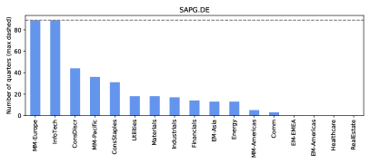
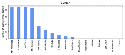
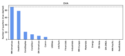
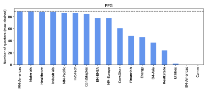
Figure 1: Correlation factor allocation. Factors are re-calibrated on a quarterly basis; the plots show how often a factor has been included. Top left: SAP is a German IT company. Top right: Amazon is a US based online retailer; however, it is also the world’s largest provider of computing services (AWS) with a strong presence in Europe. Bottom: lowest (left) and highest (right) factor allocation.

The parameters $\eta$, $\lambda_{1},...,\lambda_{d}$ and $\nu_{1}...,\nu_{d}$ are easily determined by standard regression techniques such as OLS on the transformed correlations $\text{tanh}^{-1}(c_{ij})$. The fit is computationally efficient and hence, allows the processing of very large and complex portfolios. With parameters calibrated on a regular basis, the parameter history can be used to better understand correlation dynamics and to put a plausibility constraint on correlation scenarios. Here, parameters are calibrated daily from the $250$ log-returns preceding day $t$. As outlined in Section 2.1, we test for positive-semidefiniteness and, if necessary, use the search algorithm in Higham (2002) to find the nearest correlation matrix that tests positive definite.

The heatmaps in Figure 2 show empirical correlations over 250 trading days (left) as well as the corresponding fitted correlation matrices (right), where a brighter colour indicates a higher correlation. The model is capable of capturing a number of correlation structures that are visible as shaded areas or stripes in all heatmaps. The top rows and left most columns show correlations between German DAX assets and US S&P 500 assets. Naturally, cross-country correlations are structurally lower than within country correlations.

Owing to the COVID-19 outbreak, New York City – one of the world’s largest financial centres – started to lock down on Friday, 13 March 2020. The following days saw some of the largest market drops in history. As is symptomatic for falling markets, correlations spiked during the downturn. The heatmaps, being depicted on an identical color scale, show this by jumping from a dark purple (top) to a bright orange (bottom). We will later show that this constituted, at least partially, the worst-case scenario of the portfolio. In other words, diversification benefits diminished at times where they would have been needed most.

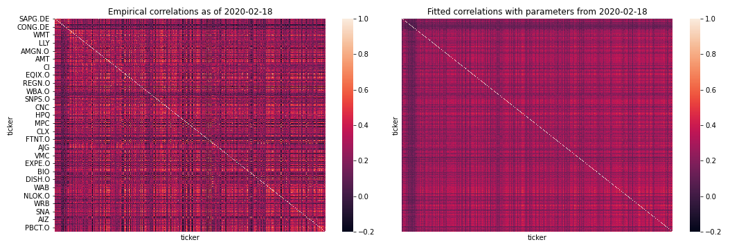
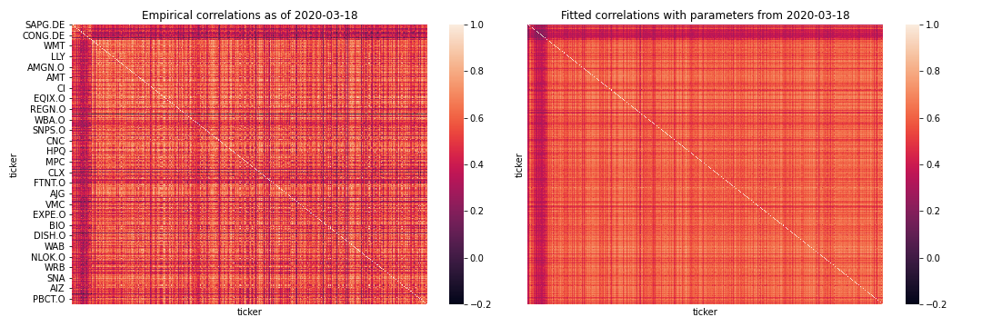
Figure 2: Heatmaps of empirical (left) and fitted (right) correlations. The spike in correlations between 18 Feb (top) and 18 Mar 2020 (bottom) was caused by markets reacting to the COVID-19 crisis. Empirical correlations are calculated on a window of 250 trading days.

The time series of fitted correlation parameters in Figure 3 shows correlation dynamics over time. One can clearly see the spikes in correlation during the financial crisis, the government debt crisis and most recently the COVID-19 pandemic. The correlation dynamics within the financial sector during 2008 are particularly interesting. The factor load on financials is almost entirely consumed by global factors as soon as the crisis spills over into the whole economy. To this end, recall the summation formula in (2), which approximates correlations in our model by sums of individual correlation risk factor loads. It is therefore natural that the (financial) sector specific correlation structure was temporarily subsumed by the more common Americas factors. For the 250 trading days leading up to the default of Lehman Brothers, the average correlation among all assets was 0.32 while the correlation within the financial sector was 0.40. The model would therefore add sector specific correlation through the corresponding “intra_Financials” factor load, which at the time was roughly 0.1. During the following 250 trading days, i.e. during the financial crisis, the average correlation increased to a level of 0.50 overall and 0.51 for financials, which explains the increase in “Americas” and decrease in “Financials” factor loads.

Figure 4 presents box-plots of coefficients of correlations between factors (left) and within factors (right). Unsurprisingly, the factor representing correlations within North America (“intra_MM-Americas”) captures the majority of the correlation dynamics in our portfolio, followed by the factor capturing correlations between North America and other countries. This shows that the method adapts well to the underlying portfolio, which comprises only US and German assets.

In general, intra-correlations are higher than inter-correlations. This is not surprising as correlations are higher for similar assets, such as assets within the same country or industry.

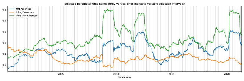
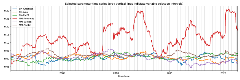
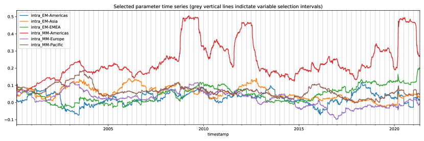
Figure 3: Top: fitted parameters for risk factors with high loads. Bottom left: fitted “inter” parameters for regional risk factors (“$\lambda_{k}$”). Bottom right: fitted “intra” parameters for regional risk factors (“$\nu_{k}$”). Grey vertical lines indicate factor selection intervals.

4.3 Stress test results

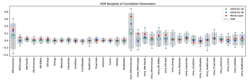
Figure 4: Reverse stress test, i.e., worst-case scenario within the $95\%$ highest density region as of 2020-02-18. Triangles indicate stress scenarios from Monte Carlo and historical simulation. The stress scenario was partially realized by 2020-03-18. Stars indicate correlation parameters for specific dates. The large shift in correlations around that time is owed to the COVID-19 crisis.

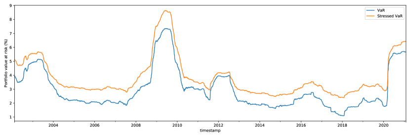
Figure 5: One day 99% VaR and stressed VaR. The stressed war uses the reverse stress scenario of 2021-05-04. The difference between both VaRs diminishes occasionally, indicating that the stress scenario has been realized.

A shift in correlation has, ceteris paribus, no instantaneous effect on a portfolio’s value, therefore, to reveal the impact of a correlation stress test requires calculating portfolio risk measures. Value-at-risk (VaR) in a variance-covariance approach has been proposed in Section 2 as a straightforward portfolio risk measure.

In order to impose a plausibility constraint on the correlation stress scenario we fit the correlation parameters to a multivariate normal-inverse Gaussian (NIG) distribution (cf. Section 2.3). The (multivariate) NIG distribution belongs to the family of normal-mean-variance mixtures, which generalise the (multivariate) normal distribution. It allows for skewness in the margins as well as a higher variation in tail behaviour compared to the normal distribution, while still being a light-tailed distribution, which is appropriate for the correlation parameters. For reasons of computation time, the NIG distribution is calibrated using every 10^th observation from the parameter data set, ie., 552 samples over time. Calibration is done using the expectation-maximization (EM) algorithm described in McNeil et al. (2005, Chapter 3), which goes back to Dempster et al. (1977). We use a Kolmogorov–Smirnov test to assess the quality of the calibration. The null hypothesis of the test is not rejected for 19 out of 34 marginal distributions at the 5% level, despite being fit to 34-dimensional data. The boxplots in Figure 4 show the range (whiskers) and inter quartile range (box) of the correlation parameters from the NIG distribution. The highest density region that is relevant for the stress test is represented by a grey area.

Figure 4 shows the worst correlation stress scenario at the 95% level. Two approaches are used to determine the stress scenario. First, historical simulation, where each empirically observed set of correlation parameters is associated with a portfolio risk metric (here VaR). The parameter constellation that yields the highest risk within the 95% quantile is indicated by a right pointing triangle. Second, Monte Carlo simulation, where we sample from the continuous parameter distribution. The sample space is then restricted to all scenarios that fulfil $f(x)\geq f_{0.05}$ (cf. Section 2.3). Within that restricted sample, the parameter constellation that produces the highest risk is indicated by a left pointing triangle.

Both, historical simulation and Monte Carlo simulation yield similar scenarios. However, the Monte Carlo scenario is more extreme, as it reaches a broader range of potential parameter constellations. In any case, the worst scenario for the test portfolio is always an increase in correlations. This result is intuitive as the portfolio at hand only benefits from naïve diversification. A hedged portfolio, on the other hand, would likely suffer under decorrelation scenarios.

Stars in Figure 4 represent correlation parameters for specific dates. One can see that on 2020-02-18 most parameters were close to the center of their distribution. One month later, on 2020-03-18, the worst case has been partially realized, as indicated by the stars shifting closer to the triangles. The parameter constellation of the correlation stress scenario itself remains unchanged because it depends primarily on the portfolio weights and the correlation risk factors associated with the portfolio constituents. This consistency of the worst case scenario is a welcome result, from a risk management perspective, as it shows that the method is capable of providing stable guidance on the risks of a specific portfolio.

Figure 5 shows the 1-day $\text{VaR}_{99\%}$ with and without stressed correlations. All VaR’s are calculated using Equation (3). Stressed VaR uses the correlation matrix from the $95\%$-stress scenario of 2021-05-04, the last day in the data. As stressed VaR measures the impact of a plausible correlation stress scenario on historical data, the difference between stressed VaR and unstressed VaR gives insights into the severity of this scenario in the recent history. Loosely speaking, the difference in VaR’s can be attributed to correlation risk. The distance between both VaRs is highest during “normal” markets (i.e., when VaR is comparably low), where it often exceeds 50% of the unstressed VaR. This is a significant value, given that the stressed portfolio is equally weighted and, thus, only benefits from naïve diversification. A portfolio that benefits from greater diversification, e.g. because it is “optimally-weighted” or hedged to minimize risks, would presumable react more sensitive to correlation changes.

During distress periods, the distance between VaR and stressed VaR diminishes, indicating that the stress scenario is at least partially realized. This can be observed during the 2008 financial crisis, the subsequent government debt crisis and most recently during the 2020 COVID-19 crisis.

5 Conclusion

Correlation, as the driver of diversification, has been extensively studied in the finance literature. For example, multivariate time series models such as DCC-GARCH capture the time variation of correlation. The more recent literature uses hierarchical clustering methods to infer dependence networks from correlation data, which allows to determine economic linkages between assets. However, other than that the literature on linking economic risk factors and correlations is scarce. Likewise, stress testing of correlations by translating an economic scenario into a change of correlations, is largely an unexplored field.

We develop a flexible correlation stress testing framework that links risk factors with asset correlations. The process consists of three steps:

First, the correlation matrix of asset returns is specified as a parametric function of risk factors, involving both “intra”- and “inter”-correlations amongst the risk factors. “Intra”-correlations are correlation contributions where assets share a risk factor, and “inter”-correlations are correlation contributions where assets do not share a risk factor. The functional form is calibrated to market data in two steps: Identifying an assets’ relevant risk factors is achieved using Bayesian variable selection, which allows to specify prior information (such as the country of the firm’s headquarter) as well as control the number of factors selected. The risk factor loadings are calibrated from an empirical correlation matrix.

Second, scenarios, in particular stress scenarios, are applied by adjusting the risk factor loadings. The impact from the correlation stress scenario is determined as the change to a risk measure such as value-at-risk, expected shortfall or any other measure that employs a correlation matrix.

Third, with correlation factor loadings calibrated on a regular basis, the parameter history can be used to better understand correlation dynamics and to put a plausibility constraint on correlation scenarios. In particular, reverse stress tests can be conducted, identifying critical risk factor scenarios for the portfolio at hand. The idea is to fit the risk factors loadings to a probability distribution and define plausible scenarios as those that lie within a given confidence level. In a multivariate setting, the range of plausible scenarios can be identified as those that lie within a certain Mahalanobis distance or highest density regions (HDR) of the average scenario. In this sense, the Mahalanobis distance and HDR can be thought of as multivariate generalisations of quantiles. The scenario with the highest risk (value-at-risk) within the confidence level represents the outcome of the reverse stress test: it is both extreme and plausible. Being able to identify the relevant risk factors of the scenario provides valuable information for portfolio managers and risk managers in order to understand the correlation risk drivers of their portfolio.

In an extensive empirical example, we calculate the stressed value-at-risk over time and identify worst-case stress scenarios. We find that these scenarios are extreme enough to pose a relevant threat from a risk management perspective, yet are common enough to be realized on several occasions in our data history.

The framework developed in this paper can be employed by any stakeholder wishing to identify the economic risk of adverse correlation changes. The method is particularly relevant to regulators, for example when approving banks’ capital models that contain factor models. Future directions of research may lead to extensions involving other kinds of risk factors, such as macroeconomic factors or latent factors (e.g. principal components).

Appendix A Normal-inverse Gaussian (NIG) distribution

The NIG distribution arises as a special case of so-called normal-mean-variance mixtures (NMVM), and more specifically as a special case of the family of Generalized Hyperbolic (GH) distributions. NMVM combine a number of useful properties, amongst them their flexibility in modelling skewness and heavy tails as well as their tractability, both for numerical calculations and simulation purposes. We refer to Section 3.2.2 of (McNeil et al., 2005) for more details.

Definition 1.

The random vector $\mathbf{X}$ is said to have a (multivariate) normal mean-variance mixture distribution if

$$\mathbf{X}\stackrel{{\scriptstyle\mathcal{L}}}{{=}}\mathbf{m}(W)+\sqrt{W}A\mathbf{Z},$$

where

1. $\mathbf{Z}\sim{\rm N}_{k}(\mathbf{0},I_{k})$;

2. $W\geq 0$ is a non-negative, scalar-valued random variable independent of $\mathbf{Z}$;

3. $A\in{\mathbb{R}}^{d\times k}$ is a matrix;

4. $\mathbf{m}:[0,\infty)\rightarrow{\mathbb{R}}^{d}$ is a measurable function.

We have

$$\mathbf{X}|W=w\sim{\rm N}_{d}(\mathbf{m}(w),w\Sigma),$$

where $\Sigma=AA^{\prime}$. A possible concrete specification of $\mathbf{m}(W)$ is

$$\mathbf{m}(W)=\mathbf{\mu}+W\mathbf{\gamma},$$ (6)

where $\mathbf{\mu}$ and $\mathbf{\gamma}$ are vectors in ${\mathbb{R}}^{d}$. If $\mathbf{\gamma}=0$, then the distribution is a NVM.

A special case are the generalized hyperbolic (GH) distributions, which are NMVM’s with mean specification (6) and mixing distribution $W\sim N^{-}(\lambda,\chi,\psi)$, a generalised inverse Gaussian (GIG) distribution. We write $\mathbf{X}\sim\text{GH}_{d}(\lambda,\chi,\psi,\mathbf{\mu},\Sigma,\mathbf{\gamma})$. The specification is not unique in the sense that scaled versions of the parameters describe the same distribution.

The NIG distribution arises as the special case where $\lambda=-1/2$. An extensive treatment of the NIG distribution is found in (Barndorff-Nielsen, 1997). Amongst other useful properties, closed formulas for the moment-generating function exist, so all moments are easily calculated; linear combinations of NIG variables are again NIG-distributed; the NIG distribution features infinite divisibility, giving rise to the NIG Lévy process, which may be represented as a Brownian motion with a random time change.

References

- Adams et al. (2017) Adams, Z., R. Füss, and T. Glück. Are correlations constant? Empirical and theoretical results on popular correlation models in finance. Journal of Banking & Finance, 84:9–24, 2017.
- Alexander and Sheedy (2008) Alexander, C. and E. Sheedy. Developing a stress testing framework based on market risk models. Journal of Banking & Finance, 32(10):2220–2236, 2008.
- Ang and Bekaert (2002) Ang, A. and G. Bekaert. International asset allocation with regime shifts. Review of Financial Studies, 15(4):1137–1187, 2002.
- Barbieri and Berger (2004) Barbieri, M. M. and J. O. Berger. Optimal predictive model selection. The Annals of Statistics, 32(3):870–897, 2004.
- Barndorff-Nielsen (1997) Barndorff-Nielsen, O. E. Normal inverse Gaussian distributions and stochastic volatility modelling. Scandinavian Journal of statistics, 24(1):1–13, 1997.
- BCBS (2006) BCBS. International convergence of capital measurement and capital standards. Technical report, Basel Committee on Banking Supervision, 2006.
- BIS (2011) BIS. Revisions to the Basel II market risk framework. Basel Committee on Banking Supervision, Bank for International Settlements, February 2011.