Combining White Light and UV Lyman-$\alpha$ Coronagraphic Images to
determine the Solar Wind Speed: the Quick Inversion Method

Abstract

Context. The availability of multi-channel coronagraphic images in different wavelength intervals acquired from the space will provide a new view of the solar corona, allowing to investigate the 2D distribution and time evolution of many plasma physical parameters, such as plasma density, temperature, and outflow speed.

Aims. This work focuses on the combination of White Light (WL) and UV (Ly$\alpha$) coronagraphic images to demonstrate the capability to measure the solar wind speed in the inner corona directly with the ratio between these two images (a technique called ”quick inversion method”), thus avoiding to account for the line-of-sight (LOS) integration effects in the inversion of data.

Methods. After a derivation of the theoretical basis and illustration of the main hypotheses in the ”quick inversion method”, the data inversion technique is tested first with 1D radial analytic profiles, and then with 3D numerical MHD simulations, in order to show the effects of variabilities related with different phases of solar activity cycle and complex LOS distribution of plasma parameters. The same technique is also applied to average WL and UV images obtained from real data acquired by SOHO UVCS and LASCO instruments around the minimum and maximum of the solar activity cycle.

Results. Comparisons between input and output velocities show overall a good agreement, demonstrating that this method that allows to infer the solar wind speed with WL-UV image ratio can be complementary to more complex techniques requiring the full LOS integration. The analysis described here also allowed us to quantify the possible errors in the outflow speed, and to identify the coronal regions where the ”quick inversion method” performs at the best. The ”quick inversion” applied to real UVCS and LASCO data allowed also to reconstruct the typical bimodal distribution of fast and slow wind at solar minimum, and to derive a more complex picture around solar maximum.

Conclusions. The application of the technique shown here will be very important for the future analyses of data acquired with multi-channel WL and UV (Ly$\alpha$) coronagraphs, such as Metis on-board Solar Orbiter, LST on-board ASO-S, and any other future WL and UV Ly$\alpha$ multi-channel coronagraph.

1 Introduction

Near the Sun, where the main acceleration of solar wind from sub- to super-sonic and super-Alfvénic flows occur (below $\sim 15-30$ R_⊙, see e.g. Goelzer et al., 2014), measurements of the expansion speed of solar wind have been possible so far only with remote sensing data. The obvious reason for this limitation is that, due to the extreme local conditions, there were no instruments capable to explore in situ this region. Most recently, thanks to the launch of the Parker Solar Probe mission (Fox et al., 2016), it became possible to explore for the first time with in situ instruments regions much closer to the Sun (down to $\sim 10$ R_⊙), but the exploration of the inner regions still requires the analysis of remote sensing data. Currently available coronagraphic data have already proven their potential, but also their limits. In particular, classical space-based coronagraph, such as the instrument on-board the Solar Maximum Mission (MacQueen et al., 1980), LASCO on-board SOHO (Brueckner et al., 1995), COR on-board STEREO (Howard et al., 2008), were limited so far to the acquisition of broad-band images in the White Light (WL). This emission, being mostly due to Thomson scattering of photospheric light from coronal electrons, is very useful to observe large-scale coronal features, but provides local information only on the plasma column density along the line-of-sight (LOS), and no local information on other plasma parameters (temperatures of different plasma species, elemental abundances, etc.).

Fortunately, this situation will change in the near future with the new generation of multi-waveband coronagraphs, whose data will provide a new view of the solar corona, and in particular of the inner regions where the main solar wind acceleration and coronal heating processes occur. In particular, the Metis coronagraph (Antonucci et al., 2020) on-board ESA Solar Orbiter mission is now providing the first ever simultaneous observations of the corona in two different spectral bands: broad-band (580-640 nm) in the WL, and narrow-band UV emission from the neutral H atoms (121.6 nm Ly$\alpha$ line), with a FOV going from 1.7 to 3.6 R_⊙ at closest approach (0.28 AU) to the Sun. Similar data will also be acquired in the near future by another coronagraph, the LST instrument (Li et al., 2019) on-board the forthcoming Chinese ASO-S mission. The great advantages for solar wind diagnostic in the combination of UV Ly$\alpha$ and WL $pB$ coronal images was first discussed by Withbroe et al. (1982) who proposed to measure the expansion speed of the neutral H atoms with the so-called Doppler dimming technique. The measurement is based on well known fact that the coronal Ly$\alpha$ emission is almost entirely due to the resonant scattering of chromospheric Ly$\alpha$ emission (Gabriel, 1971). As a consequence, a relative motion of coronal H atoms with respect to the chromosphere leads to a Doppler shift of the exciting Ly$\alpha$ profile with respect to the atomic absorption profile, reducing the efficiency of radiative excitation, and then the observed Ly$\alpha$ emission (see Vial & Chane-Yook, 2016, for a more recent review). This method is suitable for coronal features such as streamers, plumes, and coronal holes, where (thanks to the low plasma densities) the collisional Ly$\alpha$ component is negligible, which is not necessarily true for the emission associated with erupting prominences and the cores of Coronal Mass Ejections where the Ly$\alpha$ collisional component can be significant or event dominant, as demonstrated by more recent data analysis (Susino et al., 2018) and numerical MHD simulations (Bemporad et al., 2018).

The Doppler dimming technique has been successfully applied to measure the solar wind speed in the inner corona with the analysis of spectro-coronagraphic observations acquired by the UVCS instrument (Kohl et al., 1995) on-board SOHO (see Kohl et al., 2006, for a review of the main UVCS results). This kind of measurements also increases the complementarity between in situ and remote sensing data, allowing to relate plasma physical parameters measured locally with their global large-scale distribution. Nevertheless, the application of the Doppler dimming technique usually requires not only the integrated intensity of some selected spectral lines (in particular the 121.6 nm H i Ly$\alpha$ line, and the 103.2–103.8 nm O vi doublet lines), but also information on the shape of coronal profiles. Unfortunately, this information will not be provided by a coronagraph like Metis, which is not equipped with a spectroscopic channel like UVCS. Nevertheless, reliable solar wind speed measurements can be derived with Doppler dimming technique even just from the Ly$\alpha$ integrated intensity, once a corresponding WL coronagraphic image is provided. This was more recently demonstrated in Bemporad (2017), who derived 2D maps of the solar wind speed using the so-called synoptic UVCS observations (Strachan et al., 1997; Panasyuk et al., 1998) to build 2D coronagraphic Ly$\alpha$ intensity images, and then coupling these images with WL coronagraphic observations. The same images were thus used by Dolei et al. (2018) and Dolei et al. (2019) to characterize and constrain the main uncertainties in the Doppler dimming technique applied to 2D intensity images, missing the spectroscopic information.

Nevertheless, the methods applied first by Bemporad (2017), and then by Dolei et al. (2018) and Dolei et al. (2019) to the same reconstructed images were intrinsically different, as it is explained in more details below. In summary, the method applied by Bemporad (2017) (hereafter called ”quick inversion method”) was based on the analysis of the image resulting from the direct ratio between the UV and WL images, while the method applied by Dolei et al. (2018) and Dolei et al. (2019) (hereafter called ”full inversion method”) was based on a more complete analysis taking into account LOS integration effects. The aim of this paper is to review the two methods, and in particular to derive explicit expressions useful to apply the ”quick inversion method” to future observations of the corona both in the WL and UV Ly$\alpha$ bands. In particular, after a short review of the two methods (§ 2), the approximate expressions to be used are discussed in details (§ 3) both for the UV Ly$\alpha$ (§ 3.1) and the WL $pB$ (§ 3.2) images, deriving an explicit expression to measure the outflow speed and its associated uncertainty (§ 3.3). The method is finally tested with 1D synthetic emission profiles (§ 4.1), 2D synthetic images based on 3D MHD simulations (§ 4.2), and 2D images based on real observations (§ 4.3). The results, advantages and limits of the method are finally summarized and discussed (§ 5).

2 The full and quick inversion methods

2.1 Full inversion

The Doppler dimming/pumping technique has been applied in the past mostly to measure the expansion speed of heavy ions, and in particular of O⁵⁺ ions in coronal holes and coronal streamers (see reviews by Cranmer, 2002; Abbo et al., 2016, and references therein), by exploiting the fact that the ratio between O vi $\lambda\lambda$ 1031.9-1037.6 lines is mostly dependent on the ion outflow speed (Noci et al., 1987), that can be measured once the plasma electron temperature $T_{e}$ and density $n_{e}$ (plus other parameters) are known (see Zangrilli et al., 2002, for a detailed description of the method). Nevertheless, the expansion speed of heavy ions $V_{ion}$ is not representative of the solar wind bulk speed $V_{sw}$, because these ions undergo a preferential heating and acceleration, that was one of the major discoveries by UVCS experiment (see review by Kohl et al., 2006). On the other hand, the speed of the expanding protons $V_{p}$ can be measured almost directly by applying the Doppler dimming technique to the H i Ly$\alpha$ line intensity, under the assumption that protons and neutral H atoms are still coupled (hence $V_{p}\simeq V_{H}$), which is true only in the inner corona typically below $\sim 10$ R_⊙ (Withbroe et al., 1982). A decoupling in the direction perpendicular to the flow may occurr even at lower altitudes (see discussion by Allen et al., 1998), thus possibly affecting the reliability of proton kinetic temperature measurements form Ly$\alpha$ line profile (e.g. Labrosse et al., 2006).

Because coronal plasma are usually optically thin (see review by Bradshaw & Raymond, 2013), the derivation of proton speed $V_{p}$ on the plane-of-sky (POS) with the Doppler dimming of Ly$\alpha$ intensity usually requires a very complex inversion procedure, taking into account not only the (unknown) distributions along the line-of-sight (LOS) of $T_{e}$, $n_{e}$, $T_{p//}$ and $T_{p\perp}$ (i.e. temperatures parallel and perpendicular to the magnetic fieldlines), but also the LOS distribution of $V_{p}$ itself. This problem is usually solved by estimating the POS values of $T_{e}$, $n_{e}$ and $T_{p\perp}$, by assuming a spherical geometry for the LOS distributions of these parameters, by starting from a level of temperature anisotropy, and also by assuming the mass flux conservation in magnetic fluxtubes, hence an analytical (e.g. Banaszkiewicz et al., 1998) or an empirical (e.g. Vásquez et al., 2003) model for the LOS distribution of magnetic fieldlines. An iteration over the space of the free parameters (e.g. the POS speed and the anisotropy level) is then performed, until the best match between the synthetic and the observed Ly$\alpha$ intensities is obtained (see Zangrilli et al., 2002, for details). A slightly simplified version of this technique was applied by Spadaro et al. (2007) and more recently by Dolei et al. (2018) and Dolei et al. (2019), where (considering that in particular in coronal streamers the super-radial expansion of solar wind hence of magnetic fluxtubes is not very important), the assumption of a LOS distribution of magnetic fluxtubes was replaced by the assumption that the radial POS distribution of outflow speed equals the distribution along the LOS (which corresponds to assume spherical symmetry also for the velocity distribution along the LOS).

2.2 Quick inversion

The above methods have been applied by many authors to measure $V_{p}$ from the Doppler dimming of Ly$\alpha$ intensity (see Introduction and Figure 1 by Bemporad, 2017, for a quick review). Nevertheless, the significant number of needed assumptions on the LOS distributions of plasma parameters, results in significant uncertainties in the derived values for $V_{p}$. Recently, Cranmer (2020) re-analysed a large set of Ly$\alpha$ line profile measurements acquired by UVCS in 1996-1997 in a polar coronal hole to constrain (with forward modeling based on Monte Carlo method to build a posterior probability distributions) the set of plasma parameters that give the best match with the UVCS data. Surprisingly, this complete re-analysis of data previously analysed by Cranmer et al. (1999) shows that between 1.5 and 4 R_⊙ the electron temperature $T_{e}$, the proton temperature $T_{p}$, and the temperature anisotropy $T_{p\perp}/T_{p//}$ do not show substantial radial dependences, changing only by $\sim 20\%$, $\sim 84\%$, and $\sim 25\%$ respectively, hence always less than a factor $\sim 2$. The other plasma parameters are changing much more significantly over the same altitude interval: the proton outflow speed $V_{p}$ increases by a factor $\sim 4$, and more importantly the electron density $n_{e}$ decreases by almost two orders of magnitude. Moreover, coronal protons have a very little temperature anisotropy, on the order of $T_{p\perp}/T_{p//}\sim 1.06$ (see Cranmer, 2020). The same conclusions are expected to be valid also in coronal streamers, from where the slow solar wind is blowing (see Kohl et al., 2006, and references therein), and where the level of proton anisotropy is expected to be negligible everywhere except in the streamer edges and coronal hole boundaries (Frazin et al., 2003; Susino et al., 2008).

The above lines of reasoning show that, considering the LOS contribution to the coronal Ly$\alpha$ intensity, there is only one plasma physical parameter dramatically changing (i.e. by orders of magnitude) with the radial distance from the Sun: the plasma density. For this reason, over the past decades some authors used approximate expressions for the Ly$\alpha$ intensity that are considering only the LOS variations of $n_{e}$, and by assuming that no significant LOS variations of all other plasma parameters occur. Similar approximate expressions have been used for instance to measure the electron density at the base of coronal streamers (Ko et al., 2002) by assuming negligible outflows (hence neglecting Doppler dimming), but also to measure the electron temperature in Coronal Mass Ejections - CMEs (Susino & Bemporad, 2016; Ying et al., 2020), by measuring their expansion speed from coronagraphic images to constrain the Ly$\alpha$ Doppler dimming.

An approximate expression for the Ly$\alpha$ line can be derived starting from the important consideration that in the solar corona the Ly$\alpha$ emission is dominated by resonant scattering of chromospheric Ly$\alpha$ emission (Gabriel, 1971). Hence, as it was originally proposed by Kohl & Withbroe (1982), the coronal Ly$\alpha$ line can be used to measure the solar wind outflow speed directly from the ratio between its intensity and the intensity of the electron-scattered WL continuum. For this purpose, it is necessary to approximate the Ly$\alpha$ resonant scattering component $I_{res}$ as

$$I_{res}=\mathrm{const}\,\,\langle R(T_{e})\rangle\,\langle D(V_{sw})\rangle\int\limits_{LOS}n_{e}\,dz$$ (1)

where $R(T_{e})$ is the H ionization fraction (dependent on the electron temperature $T_{e}$), $V_{sw}$ is the radial component of the wind speed, $D$ is the Doppler dimming term ($0\leq D\leq 1$, with $D=1$ for $V_{sw}=0$, and $D\longrightarrow 0$ for $V_{sw}\longrightarrow\infty$), and the symbol $\langle...\rangle$ indicates the average value along the LOS across the emitting plasma; an explicit form of $D$ will be derived below.

The intensity of the polarized brightness of WL $pB$ can also be approximated as

$$I_{pB}=\mathrm{const}\int\limits_{LOS}n_{e}\,dz,$$ (2)

therefore, the ratio between the two measured quantities is almost independent on $n_{e}$, and corresponds to

$$\frac{I_{res}}{I_{pB}}=\mathrm{const}\,\,\langle R(T_{e})\rangle\,\langle D(V_{sw})\rangle.$$ (3)

The above expression implies that, given an estimate of $T_{e}$, the $I_{res}/I_{pB}$ intensity ratio can be used to measure directly $D(V_{sw})$, hence to estimate $V_{sw}$. The same technique was more recently described again by Kohl et al. (2006) and successfully applied by Bemporad (2017).

This method is relatively simple, because does not require performing iterations along the LOS based on geometrical assumptions of the unknown LOS distributions of many plasma physical parameters, as previously discussed; for this reason, it is called ”quick inversion method”. In the next section we derive the explicit expression for the Ly$\alpha$ approximate intensity used by this method.

3 Approximate expressions

3.1 Approximate Ly$\alpha$ expression

A complete review of EUV line formation processes in the solar corona was recently given by Del Zanna & Mason (2018). Here, we derive the Ly$\alpha$ intensity approximate form starting from the expression (given by Noci & Maccari, 1999, Eq. 9) for the line emissivity $j(P,\mathbf{n})$ of a radiatively excited line emitted from a scattering atom located at the coronal point $P$, after integration over the (Maxwellian) velocity distribution, which is given by

$$j(P,\mathbf{n})=h\nu_{0}\,n_{H}\frac{B_{12}}{4\pi}\!\int\limits_{\Omega}\!\!p(\phi)d\omega^{\prime}\!\!\!\int\limits_{-\infty}^{+\infty}\!\!I(\nu^{\prime}[V_{p},\nu_{0}],\mathbf{n^{\prime}})g_{p}(V_{p})dV_{p}$$ (4)

where $n_{H}$ is the number density of the absorbing H atoms, $B_{12}$ is the Einstein coefficient relative to the considered transition at frequency $\nu_{0}$, $\nu^{\prime}=\nu_{0}(1+\mathbf{n^{\prime}}\cdot\mathbf{v}/c)$ is the frequency of the absorbed photon for an observer at rest with the scattering atom moving with velocity $\mathbf{v}$ with respect to the emitting source (the Sun), $p(\phi)$ is a geometrical factor representing the probability for the photon coming from the direction $\mathbf{n^{\prime}}$ to be absorbed and re-emitted through the angle $\phi$, $\mathbf{n}$ is the LOS direction, $\Omega$ is the solid angle subtended by the solar disk at scattering point $P$, and $V_{p}=\mathbf{v}\cdot\mathbf{n^{\prime}}$ is the velocity of scattering atom projected in the direction of the incoming photon $\mathbf{n^{\prime}}$ and having normalized Maxwellian distribution $g_{p}$. The line emissivity at point $P$ needs to be integrated along the LOS coordinate $z$ to get the observed resonant scattered intensity $I_{res}$ which is given by

$$I_{res}=\int\limits_{-\infty}^{+\infty}j(P,\mathbf{n})dz$$ (5)

The above line emissivity $j$ can be integrated analytically by making a few assumptions described below. First, we assume that the excitation profile has a Gaussian shape, and thus is given by (see Noci & Maccari, 1999, Eq. 10)

$$I(\nu^{\prime}[V_{p},\nu_{0}],\mathbf{n^{\prime}})=\frac{I_{0}}{\sqrt{\pi}\sigma_{\nu}}\,\exp\left[-\frac{(\nu^{\prime}-\nu_{0})^{2}}{\sigma_{\nu}^{2}}\right]$$ (6)

and considering that $\nu^{\prime}=\nu_{0}(1-V_{p}/c)$ the above profile can be rewritten as

$$I(V_{p}) = \frac{I_{0}\,\lambda_{0}}{\sqrt{\pi}(c\,\sigma_{\nu}/\nu_{0})}\,\exp\left[-\frac{V_{p}^{2}}{(c\,\sigma_{\nu}/\nu_{0})^{2}}\right]=$$

$$= \frac{I_{0}\,\lambda_{0}}{\sqrt{\pi}s_{disk}}\,\exp\left[-\frac{V_{p}^{2}}{s_{disk}^{2}}\right]$$

where $s_{disk}=\sigma_{\nu}\,c/\nu_{0}$ [km s^-1] is $1/e$ half-width of the disk exciting profile with total intensity $I_{0}$. On the other hand, by assuming that the scattering atoms are moving radially with the bulk solar wind velocity $V_{0}$ (using the same notation as Noci & Maccari, 1999), the normalized atomic absorption profile $g_{p}(V_{p})$ can be written as

$$g_{p}(V_{p})=\frac{1}{\sqrt{\pi}s_{cor}}\,\exp\left[-\frac{(V_{p}-V_{0})^{2}}{s_{cor}^{2}}\right]$$ (8)

where $s_{cor}=\sqrt{2\,k_{B}T_{k}/m_{H}+\xi^{2}}$ [km s^-1] is the $1/e$ half-width of the absorption profile, that includes the thermal ($2\,k_{B}T_{k}/m_{H}$) and non-thermal ($\xi^{2}$) line broadening, $T_{k}$ is the kinetic temperature of the scattering ions. Note that Eq. 8 is valid in the assumption of an isotropic temperature distribution. By replacing the above expressions for $I(V_{p})$ and $g_{p}(V_{p})$ the convolution integral in Eq. 4 becomes:

$$I_{0}\lambda_{0}\int\limits_{-\infty}^{+\infty}\frac{1}{\sqrt{\pi}s_{disk}}e^{-V_{p}^{2}/s_{disk}^{2}}\frac{1}{\sqrt{\pi}s_{cor}}e^{-(V_{p}-V_{0})^{2}/s_{cor}^{2}}\,dV_{p}.$$ (9)

The above expression can be integrated analytically: as it is well-known (e.g. Bromiley, 2014) the product between two normalized Gaussian functions $g(V)$ with peak values at $V_{1}$ and $V_{2}$ and $1/e$ half-widths $s_{1}$ and $s_{2}$ is a normalized Gaussian function with mean $V_{12}=(V_{1}s_{2}^{2}+V_{2}s_{1}^{2})/(s_{1}^{2}+s_{2}^{2})$, variance $s_{12}=\sqrt{s_{1}^{2}s_{2}^{2}/(s_{1}^{2}+s_{2}^{2})}$, and multiplied by the constant

$$G_{12}=\frac{1}{\sqrt{\pi}\sqrt{s_{1}^{2}+s_{2}^{2}}}\exp{\left[-\frac{(V_{1}-V_{2})^{2}}{(s_{1}^{2}+s_{2}^{2})}\right]}$$ (10)

where in our case $V_{1}=0$ and $V_{2}=V_{0}$. Hence, the integration of Eq. 9 gives

$$\int\limits_{-\infty}^{\infty}\!\!I(\nu^{\prime}[V_{p},\nu_{0}],\mathbf{n^{\prime}})g_{p}(V_{p})dV_{p}=\frac{I_{0}\lambda_{0}\,\exp\left[-\frac{V_{0}^{2}}{(s_{disk}^{2}+s_{cor}^{2})}\right]}{\sqrt{\pi}\sqrt{s_{disk}^{2}+s_{cor}^{2}}}.$$ (11)

The expression given in Eq. 4 can be further simplified by considering that for the Ly$\alpha$ line (Noci et al., 1987)

$$p(\phi)=\frac{1}{4\pi}\frac{11+3\cos^{2}\phi}{12}\simeq\frac{1}{4\pi}$$ (12)

because the bulk of the Ly$\alpha$ emission is coming from the plasma located near the POS ($\cos\phi\simeq 0$) and the integration over the solid angle $d\omega^{\prime}$ can be factorized and simplified into

$$\int\limits_{\Omega}\!\!p(\phi)d\omega^{\prime}\simeq\frac{1}{4\pi}\Omega_{\odot}(\rho)=\frac{1}{4}h(\rho)$$ (13)

where $\Omega_{\odot}(\rho)$ is the solid angle subtended by the solar disk at scattering distance $\rho$ on the POS, and the function $h(\rho)$ is given by $h(\rho)=2\left(1-\sqrt{1-R_{\odot}^{2}/\rho^{2}}\right)$ (see e.g. Ko et al., 2002). Moreover, the number density of neutral H atoms can be rewritten as

$$n_{H}\equiv\frac{n_{H}}{n_{p}}\frac{n_{p}}{n_{e}}\,n_{e}=R_{H}(T_{e})\frac{n_{p}}{n_{e}}\,n_{e}\simeq R_{H}(T_{e})\,0.83\,n_{e}$$ (14)

where $R_{H}(T_{e})$ is the neutral Hydrogen ionization fraction, and $n_{p}/n_{e}=n_{H}/(n_{H}+2n_{He})\equiv 1/(1+2n_{He}/n_{H})\simeq 0.83$ having assumed (e.g. Del Zanna & Mason, 2018) that the considered plasma is made of a combination of 90% of Hydrogen and 10% of Helium ($n_{He}/n_{H}\simeq 0.1$).

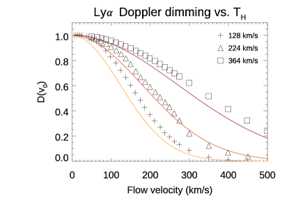
Figure 1: Comparison between the Ly$\alpha$ Doppler dimming factors as provided by Kohl et al. (1997) (Fig. 1, same symbols) and those obtained with the analytic formula given here in Eq. 17 (solid lines).

In summary, by replacing Eqs. 11, 13, and 14 into Eq. 4 it turns out that

$$j(\rho)=0.83\frac{h\,\nu_{0}B_{12}}{16\pi\sqrt{\pi}}R_{H}\left[T_{e}(\rho)\right]n_{e}(\rho)h(\rho)\times$$ (15)

$$\times\frac{I_{0}\lambda_{0}}{\sqrt{s_{disk}^{2}+s_{cor}^{2}}}\exp\left[-\frac{V_{0}^{2}}{(s_{disk}^{2}+s_{cor}^{2})}\right]$$

that can be also rewritten by replacing the observed $1/e$ half-widths of the excitation ($\sigma_{disk}(\lambda)$) and absorption ($\sigma_{cor}(\lambda)$) profiles (both assumed to be Gaussian) as

$$j(\rho)=0.83\frac{h\,\lambda_{0}B_{12}}{16\pi\sqrt{\pi}}R_{H}\left[T_{e}(\rho)\right]n_{e}(\rho)h(\rho)\times$$ (16)

$$\times\frac{I_{0}}{\sqrt{\sigma_{disk}^{2}+\sigma_{cor}^{2}}}\exp\left[-\frac{V_{0}^{2}}{(\sigma_{disk}^{2}+\sigma_{cor}^{2})c^{2}/\lambda_{0}^{2}}\right]$$

and finally, the above expression needs to be integrated along the LOS coordinate $z=\sqrt{r^{2}-\rho^{2}}$ to get the total intensity.

Moreover, the above equation provides a useful analytic expression for the Doppler dimming coefficient $D(V_{0})$ which is given by

$$D(V_{0})=\exp\left[-\frac{V_{0}^{2}}{(\sigma_{disk}^{2}+\sigma_{cor}^{2})c^{2}/\lambda_{0}^{2}}\right].$$ (17)

This is a general expression (under all the above assumptions) that holds for any coronal spectral line radiatively excited by the disk emission in the same line. A comparison between values for $D(V_{0})$ given by the above analytic expression (by assuming $1/e$ half-width of the Ly$\alpha$ chromospheric profile $\sigma_{disk}=0.34$ Å) and those given by Kohl et al. (1997) is provided in Fig. 1, showing a nice agreement between the different curves for different kinetic temperatures $T_{k}$ within $\sim 20-30$ km s^-1. This functional form of Doppler dimming coefficient was the same already used for instance by Cranmer et al. (1999) (Eq. 17) to measure the solar wind speed in polar coronal holes. Also note that, because both the excitation and absorption profiles were assumed to be Gaussian hence symmetric, the above expression for the Doppler dimming coefficient holds both for plasma escaping from the Sun ($V_{0}=V_{sw}>0$), and for plasma moving towards the Sun, as it may happen to down-flowing plasma blobs (e.g. Wang et al., 1999), but also for the cometary emission by considering the radial component ($V_{0}=V_{r;com}\gtrless 0$) of the comet velocity, an effect called ”Swings effect” (Swings, 1941).

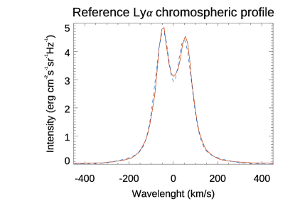
Figure 2: Reference Ly$\alpha$ chromospheric profile from Gunár et al. (2020) (solid line) and three-Gaussian fitting (dashed line).

As discussed above, in the approximate expression considered here, it will be assumed that all the main plasma physical parameters are not changing significantly along the LOS in the emitting plasma column, with the only exception to the electron density $n_{e}$, so that the total scattered intensity $I_{res}(\rho)$ at the projected distance $\rho$ from the Sun is given by

$$I_{res}(\rho)=0.83\frac{h\,\lambda_{0}B_{12}I_{0}}{16\pi\sqrt{\pi}}\,\frac{R_{H}\left[T_{e}(\rho)\right]\,h(\rho)}{\sqrt{\sigma_{disk}^{2}+\sigma^{2}_{cor}(\rho)}}D[V_{0}(\rho)]\times$$ (18)

$$\times\int\limits_{-\infty}^{+\infty}n_{e}(z)dz=H_{res}\,K_{res}(\rho)\,D[V_{0}(\rho)]\,\int\limits_{-\infty}^{+\infty}\,n_{e}(z)\,dz$$

where in the above expression all the varying quantities are written as a function of $\rho$.

It is important to notice that, as any approximation, the above expression has some limits. In particular, the assumption that the integration over the solid angle subtended by the solar disk can be simply factorized as expressed by Eq. 13 (usually referred as ”point source” approximation) fails for regions in the inner corona where different values of this solid angle in the integration along the LOS need to be taken into account. The assumption that the same value of solid angle $\Omega_{\odot}(\rho)$ applies also for plasma emitting out from the POS leads to an overestimate of the emission from these coronal regions. A correction for the errors introduced by this approximation will be discussed later.

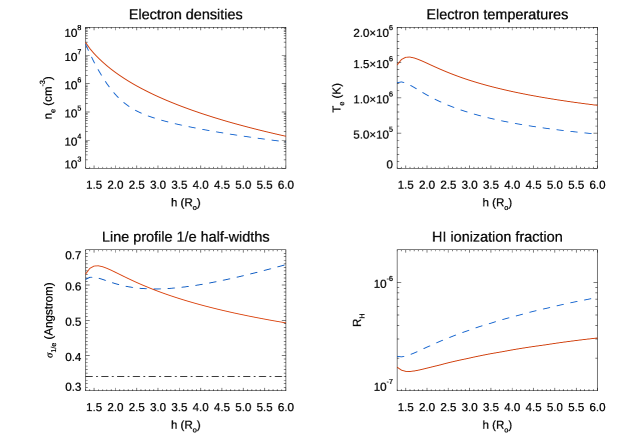
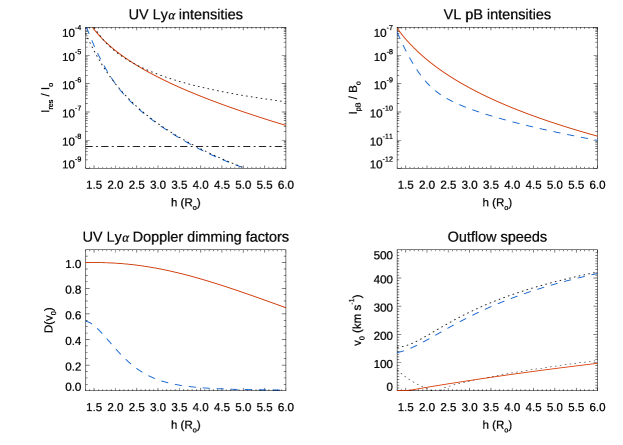
Figure 3: Radial profiles of different input and output parameters in coronal streamer (solid red lines) and coronal hole (dashed blue lines), in particular (from top left to bottom right): electron densities, electron temperatures, Ly$\alpha$ line profile widths (the dash-dotted line shows the chromospheric line widths), H i ionization fractions, $I_{res}$ Ly$\alpha$ intensities (normalized with respect to the disk intensity $I_{0}$, the dash-dotted line shows the interplanetary Ly$\alpha$ intensity, while dotted lines show typical Ly$\alpha$ intensity profiles as observed by SOHO UVCS at solar minimum), $I_{pB}$ intensities (normalized with respect to the mean solar brightness $\bar{B}_{\odot}$), $I_{res}$ Ly$\alpha$ Doppler dimming factors, and input and output (dotted lines) outflow speed ($V_{0}$) profiles.

In the analysis described above it was also assumed (as done by many previous authors) that the Ly$\alpha$ chromospheric profile can be well approximated by a single Gaussian profile. Nevertheless, as it is well-known, the Ly$\alpha$ chromospheric emission is characterized by a reversed shape around the line centre due to the absorption from H in the upper chromosphere and transition region; a reference Ly$\alpha$ disk profile was recently provided by Gunár et al. (2020). As it was shown for instance by Auchère (2005), this profile can be well approximated by the superposition of three Gaussian profiles, that can be replaced in the expression for the excitation profile (Eq. 3.1), hence in the convolution integral (Eq. 9). More recently, a reference full-disk Ly$\alpha$ chromospheric profile was published by Gunár et al. (2020); starting from the profile provided by these authors, the single Gaussian profile can be replaced by

$$I(V_{p})=\frac{\lambda_{0}}{\sqrt{\pi}}\,\left[i_{0}e^{-\frac{V_{p}^{2}}{s_{disk0}^{2}}}+i_{1}e^{-\frac{V_{p}^{2}}{s_{disk1}^{2}}}+i_{2}e^{-\frac{(V_{p}-V_{2})^{2}}{s_{disk2}^{2}}}\right]$$ (19)

having assumed that only one of the three Gaussian profiles is shifted with respect to the reference central wavelength $\lambda_{0}$. In particular, the fitting curve (shown in Fig. 2) corresponds to $i_{0}=5.712$, $i_{1}=0.930$, and $i_{2}=-3.085$ erg cm^-2s^-1sr^-1Hz^-1, $s_{disk0}=68.67$, $s_{disk1}=193.52$, $s_{disk2}=46.11$ km s^-1, and $V_{2}=0.914$ km s^-1. By replacing the above expression for the exciting profile $I(V_{p})$ into the convolution integral (Eq. 9) it is possible to derive a more refined expression for the Doppler dimming coefficient $D[V_{0}(\rho)]$, that will result in the sum of three exponential terms similar to the single one given in Eq. 17, whith the only disadvantage that it is not possible any more to derive an explicit solution for the plasma flow velocity $V_{0}$.

3.2 Approximate pB expression

The derivation of an approximate expression for the WL polarized brightness ($pB$) is more straightforward, because this quantity depends only on the integration along the LOS of $n_{e}$ multiplied by some geometrical functions depending only on the heliocentric distance $r$. In particular, by assuming that in the available $pB$ image the F-corona emission due to scattering by interplanetary dust has been entirely removed, hence the K-corona emission has been isolated, the $I_{pB}(\rho)$ intensity observed at the projected distance $\rho$ on the POS is given by (van de Hulst, 1950)

$$I_{pB}(\rho)=\frac{\pi}{2}\,\sigma_{T}\,\bar{B}_{\odot}\,\int\limits_{-\infty}^{+\infty}\,n_{e}(z)\,\left[\frac{(1-u)A(r)+uB(r)}{1-u/3}\right]\,\frac{\rho^{2}}{r^{2}}\,dz$$ (20)

where $z=\sqrt{r^{2}-\rho^{2}}$, $u=0.63$ is the limb darkening coefficient in the visible wavelength of interest, $\bar{B}_{\odot}$ is the mean solar brightness in the considered wavelength band, and the expressions for functions $A(r)$ and $B(r)$ are given by Billings (1966). In order to apply the quick inversion method described in the previous section, it is necessary to assume that the above expression can be simplified into

$$I_{pB}(\rho)=\frac{\pi}{2}\,\sigma_{T}\,\bar{B}_{\odot}\,K_{pB}(\rho)\int\limits_{-\infty}^{+\infty}\,n_{e}(z)\,dz$$ (21)

where $K_{pB}(\rho)=[(1-u)A(\rho)+uB(\rho)]/(1-u/3)$. Defining the constant quantity $H_{pB}=\pi/2\,\sigma_{T}\,\bar{B}_{\odot}$, the polarized brightness will be conveniently approximated by

$$I_{pB}(\rho)=H_{pB}\,K_{pB}(\rho)\int\limits_{-\infty}^{+\infty}\,n_{e}(z)\,dz.$$ (22)

an expression that will be used in the next Section to derive an explicit expression for the outflow speed $V_{0}$.

Similar to Ly$\alpha$, also the above approximate expression for $pB$ may lead to wrong estimates of the expected intensity. In particular, as it is possible to verify numerically by assuming well-established electron density radial profiles $n_{e}(r)$ from the literature for coronal streamers (Gibson et al., 1999) and coronal holes (Cranmer et al., 1999), this approximated expression for $pB$ provides in general an overestimate by a factor of $1.2-1.6$. This may lead to wrong estimates of the outflow velocity $V_{0}$; corrections for these errors will be discussed later.

3.3 Outflow velocity measurement

Finally, Eqs. 18 and 22 can be combined into

$$\frac{I_{res}(\rho)}{I_{pB}(\rho)}=\frac{H_{res}}{H_{pB}}\frac{K_{res}(\rho)}{K_{pB}(\rho)}D[V_{0}(\rho)]$$ (23)

and, by using Eq. 17, it is possible to derive an explicit form for the velocity $V_{0}$ given by

$$V_{0}(\rho)=\sqrt{\left[s_{disk}^{2}+s_{cor}^{2}(\rho)\right]\ln\left[\frac{H_{res}K_{res}(\rho)I_{pB}(\rho)}{H_{pB}K_{pB}(\rho)I_{res}(\rho)}\right]}$$ (24)

where $s_{disk}=\sigma_{disk}\,c/\lambda_{0}$ and $s_{cor}=\sigma_{cor}\,c/\lambda_{0}$. The above expression can be used to measure the POS radial velocity of plasma pixel-by-pixel from the ratio between the $I_{res}$ and $I_{pB}$ intensity images, but only for regions where

$$\frac{I_{pB}}{H_{pB}K_{pB}}\geq\frac{I_{res}}{H_{res}K_{res}}$$ (25)

that, by looking at Eq. 23, simply corresponds to the condition that $D[V_{0}(\rho)]\leq 1$ as expected.

The advantage of the derived explicit expression (Eq. 24) for the outflow speed $V_{0}$ is also that this can be differentiated to estimate the dependence of the relative uncertainty $\Delta V_{0}/V_{0}$ on the relative uncertainties on the other quantities. It turns out that

$$\frac{\Delta V_{0}}{V_{0}}=\frac{s_{disk}\Delta s_{disk}+s_{cor}\Delta s_{cor}}{s_{disk}^{2}+s_{cor}^{2}}+\frac{\frac{\Delta I_{0}}{I_{0}}+\frac{\Delta R_{H}}{R_{H}}+\frac{\Delta I_{pB}}{I_{pB}}+\frac{\Delta I_{res}}{I_{res}}}{2\ln\left[\frac{H_{res}K_{res}I_{pB}}{H_{pB}K_{pB}I_{res}}\right]}.$$ (26)

Considering that, by assuming for instance $\Delta s_{disk}/s_{disk}\simeq\Delta s_{cor}/s_{cor}$ the first therm simply reduces to $\Delta s_{cor}/s_{cor}$, the above expression shows that the dependence of $\Delta V_{0}/V_{0}$ on the relative uncertainties on the other quantities is not linear, because each one of these uncertainties is divided by a factor that could be larger or smaller than unit depending on the considered heliocentric distance and coronal feature. The above equation shows that the main uncertainties on $V_{0}$ are not only related with those on the widths of coronal ($\sigma_{cor}$) and disk ($\sigma_{disk}$) line profiles, and on the uncertainties on the measured WL ($I_{pB}$) and UV ($I_{res}$) intensities, but also on the values of UV parameters $H_{res}$ and $K_{res}$, while the corresponding WL parameters $H_{pB}$ and $K_{pB}$ are well know. As given in Eq. 18, the former are related with the uncertainties on the knowledge of the disk intensity $\Delta I_{0}/I_{0}$ seen by the scattering atoms, and the Hydrogen ionization fraction $\Delta R_{H}/R_{H}$, dependent on the electron temperature $T_{e}(\rho)$ (see also Dolei et al., 2018, Fig. 11 and related discussion).

Some additional considerations about the described method are also important. First, even if the estimate of the ratio between the $I_{res}$ and $I_{pB}$ intensities requires converting the WL intensity from the usual relative units [$1/\bar{B}_{\odot}$] to the absolute units [phot cm^-2s^-1sr^-1], the constant $H_{pB}$ in the above equations also contains the quantity $\bar{B}_{\odot}$, and in the end the measurement of $V_{0}$ turns out to be independent on the value of $\bar{B}_{\odot}$. Second, all the above expressions assume to employ the observed polarized brightness $I_{pB}$, but in principle also the total brightness $I_{tB}$ can be used, as far as a good correction for the additional emission due to the F-corona is implemented. Third, it is also very important to point out that at larger distances from the Sun (typically above $\sim 4$ R_⊙ in polar coronal holes and above $\sim 10$ R_⊙ in coronal streamers) the Ly$\alpha$ emission is dominated by the interplanetary emission, and a reliable measurement of the outflow speed will be more difficult. Moreover, this background emission is not uniformly distributed around the sky, and is also changing with the solar rotation (see e.g. Bertaux et al., 2000, Fig. 1) and with the solar activity cycle, as clearly shown by measurements acquired with the SOHO SWAN instrument (see e.g. QuéMerais et al., 2006, Fig. 4).

4 Testing the quick inversion method

4.1 Test with 1D radial profiles

The first test on the inversion method was performed by assuming from the literature analytic 1D radial profiles for different plasma parameters inside a typical coronal streamer and coronal hole at the minimum of solar activity cycle. In particular, for this work the $n_{e}$ profiles were assumed from Gibson et al. (1999) and Cranmer et al. (1999) respectively for coronal streamer and coronal hole, the $T_{e}$ profiles from Vásquez et al. (2003) for both coronal streamer and coronal hole, the $V_{0}$ profile from Cranmer et al. (1999) for coronal hole, the $\xi$ profile from Cranmer (2020) for coronal hole (no turbulent velocity was assumed for coronal streamer). For the outflow speed in coronal streamer the following analytic expression was used

$$V_{0}(\rho)=\frac{74.3\,\rho-113.4}{0.135\,\rho+2.61}\,\,\,\mathrm{[km/s]}$$ (27)

(with $\rho$ expressed in R_⊙) that was derived from a fitting of measurements given by Strachan et al. (2002) and Noci & Gavryuseva (2007), and is valid only for $\rho>1.53$ R_⊙. Moreover, it assumed not only temperature isotropy, but also thermodynamic equilibrium so that $T_{e}=T_{k}$. All these radial profiles are shown in Fig. 3. Other constant quantities that have been assumed are the Ly$\alpha$ disk intensity ($I_{0}=5\times 10^{15}$ phot cm^-2s^-1sr^-1), and the $1/e$ half-width of the Ly$\alpha$ chromospheric profile ($\sigma_{disk}=0.34$ Å).

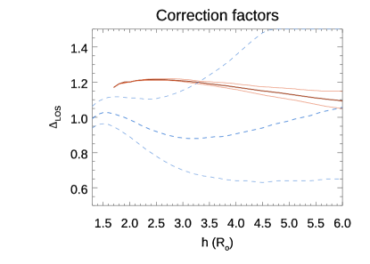
Figure 4: Radial profiles of correction factors $\Delta_{LOS}$ as derived for coronal streamer (solid red lines) and coronal hole (dashed blue lines). For each profile the upper/lower curves show the values of $\Delta_{LOS}$ parameter resulting by introducing a $\pm 5$% error on the measured velocities.

Starting from these input quantities, both the $I_{res}$ Ly$\alpha$ and $I_{pB}$ intensities have been synthesized at different altitudes $\rho$ and over $\pm 10$ R_⊙ along the LOS at each altitude, and then integrated along the LOS; the resulting output radial profiles of $I_{res}$ Ly$\alpha$ are in very good agreement with measurements acquired by the SOHO UVCS instrument (Giordano, 2011), as shown in Fig. 3 (middle left panel). In the integration along the LOS the analytic radial profiles for different plasma parameters have been used to derive at each altitude their LOS distribution, hence compute the $I_{res}$ emissivity and $I_{pB}$ intensity emitted along the LOS for the integration. In particular, the electron temperatures have been used to determine the fraction of neutral H atoms based on the ionization equilibrium curve provided by the CHIANTI spectral code (Dere et al., 2019). Then, the $I_{res}$ Ly$\alpha$ and $I_{pB}$ intensities (Fig. 3, middle panels) have been analysed by using the ”quick inversion” technique described in the previous Section, to measure the outflow speed (Eq. 24) and simulate the inversion of real data. Finally, a direct comparison between the input and the output outflow speed profiles allows testing and quantifying the accuracy of the inversion method. Nevertheless, the use of approximate Ly$\alpha$ and $pB$ expressions provided respectively in Eq. 18 and Eq. 22 inevitably introduces errors in the determination of the outflow speed $V_{0}$. Fortunately, because both approximate expressions are expected to overestimate the resulting intensity in the two spectral ranges, but the ”quick inversion” method estimates the outflow speed from the ratio between the two (Eq. 24), these two errors tend to cancel out.

Hence, to optimize the velocity measurements we introduce here a correction factor $\Delta_{LOS}$, multiplying in Eq. 24 the ratio between $I_{pB}$ and $I_{res}$ values by this factor. Then, by iterating over $\Delta_{LOS}$ values in the range between $0.5-2.0$, we measured at any altitude the value of this correction factor making the outflow velocities measured with the ”quick inversion” method coincident with the assumed input values, both for coronal streamer and coronal hole cases. This allowed us to estimate at any altitude the needed correction for the ratio between $I_{pB}$ and $I_{res}$. Values of $\Delta_{LOS}$ derived with this analysis are shown in Fig. 4, together with the corrections needed by assuming an uncertainty by $\pm 5$% on the outflow speed. Results show first of all that the uncertainties in coronal holes (dashed blue lines) are expected to be smaller with respect to coronal streamers (solid red lines), because a larger interval of possible $\Delta_{LOS}$ values allow measuring in output the same input velocities with an uncertainty below 5%. Moreover, a constant value $\Delta_{LOS}\simeq 1.2$ provides the best compromise both for coronal streamers at lower altitudes and coronal holes at higher altitudes. Hence, because our purpose is to provide a general method applicable to any coronagraphic image and any coronal structure, in what follows we will assume this value as the best compromise.

Finally, the outflow velocities $V_{0}$ resulting by applying Eq. 24 with a constant correction factor $\Delta_{LOS}=1.2$ are given in the bottom right panel of Fig. 3 (dotted red and blue lines) and compared with input velocities for a coronal streamer (solid red line) and a coronal hole (dashed blue line) Results from this simple 1D analysis show that in general the speeds measured with the ”quick inversion method” will reproduce the input velocity profiles with very small errors (less than $\sim 20$ km s^-1), both in coronal streamers and coronal holes. More in details, larger discrepancies could result only in the inner regions of coronal streamers below $\sim 2$ R_⊙, where the resulting speeds could be overestimated. The possible reason for these discrepancies will be discussed later on.

4.2 Test with 3D MHD simulations

In order to test also the effects of LOS integration once the hypothesis of cylindrical symmetry is removed, in this work a second test was performed based on 3D numerical MHD simulations. In particular, the 3D datacubes with all the main plasma physical parameters in the inner corona are freely distributed by the Predictive Science Group. These reconstructions start from the photospheric magnetic field measurements acquired by the HMI instrument on-board the SDO mission (Scherrer et al., 2012) and are based on the well-established Magnetohydrodynamic Algorithm outside a Sphere (MAS) model (see e.g. Mikić et al., 1999; Linker et al., 1999). The 3D datacubes were selected, downloaded, and managed by using the FORWARD data package freely distributed with SolarSoftware (Gibson et al., 2016), that also allows to create synthetic images in many different wavebands simulating the view from the Sun-Earth line for a specific date. This datapackage, thanks to a collaboration during a dedicated ”ISSI International Team”, was upgraded in order to include also the computation of the Ly$\alpha$ coronal emission, based on the method originally developed by Fineschi et al. (1993) to measure the coronal magnetic fields by taking advantage of the modification induced in the linear polarization of this emission line by the Hanle effect (Bommier & Sahal-Brechot, 1982). In particular, the synthetic Ly$\alpha$ intensity is calculated with the same Equations given in Sections 2.1 and 2.2 of Khan et al. (2011), by performing the full integration over the solid angle of the solar disk and along the LOS, and by approximating the wavelength integration with the same expression given here by the convolution of two Gaussian profiles (Eq. 11).

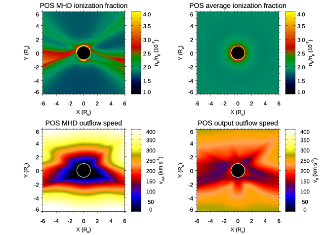
Figure 5: From top to bottom, and from left to right: synthetic WL (pB) and UV (Ly$\alpha$) images, the POS temperature distribution and the resulting averaged profile, the corresponding POS distribution of neutral H atoms and the resulting averaged distribution, and input and output outflow speeds on the POS. These panels refer to the simulation performed close to the minimum of solar activity cycle.

For this work, we selected two specific dates corresponding to the times when two different Total Solar Eclipses occurred on Earth (in order to have also possible comparisons on the appearance of the real inner solar corona in the WL images acquired from the ground). In particular, the selected dates correspond to the eclipses that occurred on 2017 August 21 (17:33 UT) near the minimum of solar activity cycle, and on 2012 November 13 (22:13 UT) near the maximum of solar activity cycle. This allows to test the inversion method in two different conditions, when the 3D structure of the solar corona is closer (near minimum) or farther (near maximum) from the cylindrical symmetry. For each one of these two dates, the synthetic WL ($pB$) and UV (Ly$\alpha$) images were built taking into account the LOS integration. Then, in order to perform the data analysis, and to take into account that the inversion of the real data will be performed without a clear knowledge of different temperatures in the real corona, the plasma temperatures in the model were extracted on the POS and averaged over all latitudes, in order to employ only the same radial temperature profile at all latitudes. This 2D average temperature maps were thus used to reconstruct (based on the usual assumption of ionization equilibrium) the 2D distribution of neutral H atoms on the POS. Finally, the ”quick inversion method” was applied pixel-by-pixel to the synthetic images to determine the 2D distribution of outflow speed on the POS, and the results were compared with the real plasma velocities extracted from the model on the POS. For this 3D test a correction factor $\Delta_{LOS}=1.2$ as derived above was used in the analysis.

Results are shown in Fig. 5 and Fig. 6 for the solar minimum and solar maximum conditions, respectively. The UV Ly$\alpha$ intensities were computed by assuming a chromospheric intensity $I_{0}=5.24\cdot 10^{15}$ phot cm^-2s^-1sr^-1. The same $I_{0}$ intensity was assumed here for both cases independently on the phase of the solar activity cycle, because by using exactly the same value also for the data inversion, this makes the results independent on the value of $I_{0}$. Bottom panels of Fig. 5 and Fig. 6 show a direct comparison between the 2D distribution of POS outflow speed in the MHD model (left) and the output POS speed as derived with the ”quick inversion method”. Obviously, the plasma physical parameters in the MHD numerical models have for each pixel in the 2D synthetic UV and WL images a 3D distribution along the LOS which is in general unknown. In particular, the MHD model has different LOS velocities that are not shown in the bottom left panels of Fig. 5 and Fig. 6. The inversion method is expected to be affected by this LOS integration effects as much as the real 3D distribution of coronal plasma parameters departs from a cylindrical symmetric distribution.

In general, Fig. 5 and Fig. 6 show that the output maps of outflow speeds allows to identify the 2D distribution of coronal regions characterized by fast and slow wind streams. This is more evident for the solar minimum condition (Fig. 5), where the clear fast/slow wind dichotomy is well reproduced around polar/equatorial regions, respectively. The situation becomes more complex for the solar maximum condition (Fig. 6), where in any case the morphological distribution of different wind streams is reproduced. On the other hand, the main problems are related with the absolute values resulting from the analysis. The measured velocities appear to be slightly underestimated in the outer corona, and also overestimated in the inner corona typically below $\sim 2$ R_⊙ (see also reference values in the bottom right panel of Fig. 3). A more quantitative comparison is shown by different panels of Fig. 7, showing that at solar minimum (left column) the velocities are slightly underestimated at 5.0 R_⊙ (bottom left panel) and overestimated at 2.5 R_⊙ (top left panel), while at solar maximum (right column) the velocities are in quite good agreement at 5.0 R_⊙ (bottom right panel) and significantly overestimated at 2.5 R_⊙ (top right panel). The possible reason for these discrepancies will be discussed later on.

4.3 Test with real observations

A further and last test of the ”quick inversion method” described here was performed based on real data acquired by the LASCO (Brueckner et al., 1995) and UVCS (Kohl et al., 1995) instruments on-board SOHO. Again, two different time periods were selected, to test the data analysis during two different phases of the solar activity cycle. In particular, the daily LASCO-C2 $pB$ images were downloaded according to the most recent version of instrument radiometric calibration (see e.g. Lamy et al., 2020) to avoid possible residual stray light in LASCO $pB$ images that could be responsible for an overestimate of $I_{pB}$, and finally for an overestimate of the outflow speed according to Eq. 24. For the test described here we focused over the time periods corresponding to Carrington Rotations 1910 (from 1996 June 1, 11:58 UT to June 28, 16:43 UT, hence at the minimum of solar activity cycle), and 1963 (from 2000 May 17, 02:55 UT to June 13, 07:51 UT, hence at the maximum of solar activity cycle). The resulting average WL $pB$ images are shown in the left panels of Fig. 8.

For the same time intervals, the averaged Ly$\alpha$ coronal intensity maps were built by collecting all together the spectroscopic observations acquired by the UVCS instrument at different latitudes and altitudes, and then by interpolating and extrapolating the Ly$\alpha$ intensities with power law fitting to fill the data gaps; a similar method was also applied by Bemporad (2017) to analyze one full solar rotation period with the UVCS Ly$\alpha$ acquired with the so-called synoptic observations (see e.g. Giordano & Mancuso, 2008). In the analysis presented here the Ly$\alpha$ intensities were extrapolated in the range between 1.5 and 4.0 R_⊙; resulting average UV Ly$\alpha$ images are shown in the middle panels of Fig. 8. Because on the other hand the LASCO $pB$ images are going from 2.1 to 6.0 R_⊙, the combined analysis with the ”quick inversion method” provides solar wind velocity maps in the range between 2.1 and 4.0 R_⊙, as shown in the right panels of Fig. 7.

In particular, the ”quick inversion method” has been applied here by assuming chromospheric Ly$\alpha$ intensities of $I_{0}=5.66\cdot 10^{15}$ and $I_{0}=8.24\cdot 10^{15}$ phot cm^-2s^-1sr^-1 as measured by the SOLSTICE satellite (Rottman et al., 2001) during CR1910 and CR1963, respectively, and in agreement with most recent data re-calibration (Machol et al., 2019). Coronal electron temperature radial profile has been assumed at all latitudes equal to an average between the profiles given by Cranmer et al. (1999) and Gibson et al. (1999) for the polar and equatorial regions, respectively. The resulting 2D electron temperature map has been converted into a neutral Hydrogen map by assuming again ionization equilibrium from CHIANTI. An interplanetary Ly$\alpha$ intensity by $I_{interp}=3.0\cdot 10^{7}$ phot cm^-2s^-1sr^-1 as provided by Kohl et al. (1997) has been subtracted from both the reconstructed coronal Ly$\alpha$ images. Again, the results for the outflow speed have been optimized by assuming a correction factor $\Delta_{LOS}=1.2$ as previously derived.

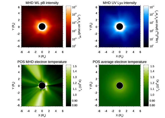
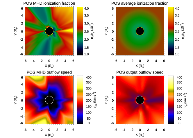
Figure 6: Same as for Fig. 5, regarding the simulation performed close to the maximum of solar activity cycle.

The outflow speed maps from application of the ”quick inversion method” are shown in the right panels of Fig. 8 for Carrington Rotations 1910 (top) and 1963 (bottom). The plots show that in both cases it was possible to derive the 2D distribution of POS outflow velocities, and the resulting maps shows very well the locations of higher and lower velocities in nearby solar wind streams. In particular, while the outflow speed map for the minimum of solar activity cycle (top right panel) clearly shows the classical bi-modality of solar wind (with fast/slow wind streams limited at the polar/equatorial regions), the map around the maximum of solar activity cycle (bottom right panel) shows faster/slower streams located at all latitudes, as expected. Moreover, the very high velocities observed during solar minimum around the polar regions are never reached at any latitude around solar maximum: this result is also confirmed by most recent solar wind speed measurements provided in different phases of the solar activity cycle and obtained in the extended corona with Fourier filtering applied to LASCO-C3 images (Cho et al., 2018), and much farther from the Sun with radio scintillation measurements (Sokół et al., 2013). In any case, we expect that these measurements will be partially affected by errors similar to those that have been found from the analysis of synthetic images and described before (end of Section 4.2). In the near future we plan to apply this method to re-analyze all the UVCS observations and provide to the community a catalogue of 2D solar wind speed maps for many different Carrington rotations between 1996 and 2002.

Figure 7: Polar plots of the POS outflow speeds as provided in input from the model (solid lines) and as resulting in output from the ”quick inversion method” (dashed lines), for the solar minimum (left column) and solar maximum (right column) conditions. The plots show the polar distributions at constant heliocentric distances of 2.5 R_⊙ (top row) and 5.0 R_⊙ (bottom row).

5 Discussion & conclusions

In this work the possible application of an inversion technique was described and tested with analytic profiles, numerical MHD simulations, and real observations. It is also important to notice that the direct ratio technique (called ”quick inversion method”) not only will provide with a few steps reliable determination of the plasma outflow speeds in the corona, but will also have many advantages with respect to the classical ”full inversion method”, that are listed here.

• Possible uncertainties related with the derivation of coronal electron densities are entirely avoided, because the velocities are derived directly from the intensity ratio in the two spectral bands.

• Possible smaller scale inhomogeneities in the outflow speed in the radial direction are detectable down to the projected pixel size, because the velocity in each pixel is independent of the nearby pixels, while the full LOS integration method is based on power law density profiles derived with geometrical assumptions, and a similar assumption is made also in the outflow speed profiles, thus significantly smoothing the possible pixel-by-pixel speed inhomogeneities.

• Images acquired during the transit of small (e.g. blobs, jets, etc.) or large (Coronal Mass Ejections, shocks, etc.) scale impulsive and transient events can be analysed as well with the direct ratio technique, because the method derives a measure of the outflow speed pixel by pixel independently, which is not true for the full inversion method which is based on power law fitting of the density profile and assumptions about the LOS integration that are not applicable to localized plasma features.

• The projected radial extension of the instrument field of view in coronagraphic images is used entirely from the inner to the outer edges of the images, while the method performing the full integration along the LOS requires assuming for a given thickness along the LOS the velocities measured on the POS, and this assumption cannot be made for pixels located closer to the outer edge of the images.

• Possible residual instrumental artefacts not removed by the absolute radiometric calibrations tend to cancel out in the direct intensity ratio, as far as the pattern of these artefacts (e.g. stray light, residual vignetting, etc.) are similar in the two channels; this is something that one may expect for the Metis instrument (Liberatore et al., 2021), considering that a significant amount of the optical path is shared for the two channels, while the same is not necessarily true for other instruments.

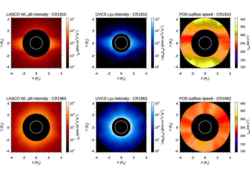
Figure 8: The average LASCO WL $pB$ (left panels) and UV Ly$\alpha$ (middle panels) images obtained for Carrington Rotations 1910 (top row) and 1963 (bottom row), and the corresponding distribution of POS speeds as derived with the ”quick inversion method” (right panels).

Nevertheless, the analysis described here also shows that the ”quick inversion method” has also significant limitations. In particular, even if the method is able to reproduce the 2D distribution of higher and lower velocities on the POS, the absolute values are expected to be slightly underestimated in the outer corona (above $\sim 2$ R_⊙) and significantly overestimated in the inner corona (below $\sim 2$ R_⊙). The sources of these two different uncertainties are totally different and are briefly discussed here. In the outer corona, as the solar wind velocities increasing with altitude approaches the value of about $\sim 300$ km s^-1, the Doppler dimming technique with Ly$\alpha$ line starts to be insensitive to higher velocities. The reason is that above this velocity the values of the Doppler dimming coefficients (Fig. 1) asymptotically goes to zero, making the measurement more and more uncertain. This is particularly true in coronal holes (see Doppler dimming values in the bottom left panel of Fig. 3), but also velocities measured in coronal streamers are affected at higher altitudes (bottom left panel of Fig. 7). It is important to notice that this limit will affect the wind speed measurements obtained both with the ”quick inversion” and the ”full inversion” methods, because this limitation is intrinsically related with the variations of Doppler dimming coefficient as a function of the outflow speed.

On the other hand, the uncertainties in the velocity determinations in the inner corona are mainly due to the approximations performed in the ”quick inversion method”, and related to the LOS integration that is neglected by the method. In particular, for the ”quick inversion” it was assumed that the integration over the solid angle subtending the solar disk can be simply factorized as expressed by eq. 13, usually referred as ”point source” approximation. Obviously, this approximation fails for regions in the inner corona, where different values of this solid angle in the integration along the LOS need to be taken into account. This source of error is peculiar of the ”quick inversion” and is not present in the ”full inversion” method. Hence, this leads us to conclude that while the method is applicable for instance to Metis data (considering that the instrument FOV will never observe the inner corona below 1.7 R_⊙), care must be taken by applying this method also to future images that will be acquired by the LST instrument, whose FOV will extend down to the solar limb. A possible modification of the ”quick inversion method” to remove this source of errors will be considered in a future work. Please also notice that this effect likely led to an overestimate of the solar wind velocities in the inner corona as published by Bemporad (2017). Despite these source of uncertainties, the ”quick method” described here could be used in principle also to discriminate from real data analysis between different models for the solar wind acceleration. To demonstrate this capability will need to create synthetic data starting from different numerical models (with different physical treatments of the solar wind), and then to invert these data with the method described here to compare finally different results. This interesting analysis goes beyond the purposes of the present work, and will be considered as a future development.

Before concluding, it is also interesting to point out that, when large or small scale parcels of plasma propagating through the corona (e.g. blobs, jets, CMEs, etc.) will be detected, the explicit expression for the outflow speed (Eq. 24) provided here can be reversed to measure the evolution of plasma temperatures. In fact, if we assume that by tracking the plasma feature (propagating inward or outward the corona) in coronagraphic images it is possible to measure (on the POS) the radial velocity profile $V_{0}(\rho)$ as a function of distance $\rho$ (or as a function of time), this also provides the evolution of the H ionization fraction which is given by

$$R_{H}[T_{e}(\rho)]=\frac{H_{res}}{H_{pB}}\frac{I_{res}(\rho)}{I_{pB}(\rho)}\frac{K_{pB}(\rho)}{h(\rho)}\frac{\sqrt{\sigma_{disk}^{2}+\sigma_{cor}^{2}(\rho)}}{\exp\left[-\frac{V_{0}^{2}(\rho)}{(\sigma_{disk}^{2}+\sigma_{cor}^{2}(\rho))c^{2}/\lambda_{0}^{2}}\right]}.$$ (28)

The application of the above expression requires first of all to measure the excess brightnesses of moving plasma features both in WL and UV (in order to remove contamination from the emitting plasma aligned with the external corona along the LOS); moreover, it is also necessary to make some assumptions on the evolution of quantity $\sigma_{cor}(\rho)=\lambda_{0}/c\sqrt{2k_{B}T_{k}(\rho)/m+\xi^{2}(\rho)}$. Once with the above expression the $R_{H}[T_{e}(\rho)]$ curve is measured, this can be reversed to measure the $T_{e}(\rho)$ curve, considering that for $T_{e}$ between $10^{6}$ and $10^{8}$K the ionization equilibrium curve provided by the CHIANTI spectral code (Dere et al., 2019) can be fit to about 10% accuracy by

$$T_{e}\simeq 0.59\cdot 10^{6}\,\,R_{H}^{-0.9407}$$ (29)

as recently provided by Cranmer (2020) (Eq. 7). Hence, the ”quick inversion method” described here has the advantage to be applicable in theory also to investigate the thermodynamic evolution of plasma erupting from the Sun at any spatial scale from large- to small-scale eruptions. The method can be applied under the hypotheses that 1) ionization equilibrium is still present, and 2) that the observed Ly$\alpha$ emission is entirely due to radiative excitation alone. These two hypotheses are not necessarily verified in the whole volume of CMEs (see discussions by Susino et al., 2018; Bemporad et al., 2018; Pagano et al., 2020), but could be verified for small-scale less energetic phenomena such as propagating plasma blobs or density inhomogeneities. This possible application of the ”quick inversion method” will be tested with MHD numerical simulations and real observations in future works.