Signed Barcodes for Multi-Parameter Persistence via Rank Decompositions and Rank-Exact Resolutions

Abstract.

In this paper we introduce the signed barcode, a new visual representation of the global structure of the rank invariant of a multi-parameter persistence module or, more generally, of a poset representation. Like its unsigned counterpart in one-parameter persistence, the signed barcode encodes the rank invariant as a ${\mathbb{Z}}$-linear combination of rank invariants of indicator modules supported on segments in the poset. It can also be enriched to encode the generalized rank invariant as a ${\mathbb{Z}}$-linear combination of generalized rank invariants in fixed classes of interval modules. In the paper we develop the theory behind these rank invariant decompositions, showing under what conditions they exist and are unique—so the signed barcode is canonically defined. We also connect them to the line of work on generalized persistence diagrams via Möbius inversions, deriving explicit formulas to compute a rank decomposition and its associated signed barcode. Finally, we show that, similarly to its unsigned counterpart, the signed barcode has its roots in algebra, coming from a projective resolution of the module in some exact category. To complete the picture, we show some experimental results that illustrate the contribution of the signed barcode in the exploration of multi-parameter persistence modules.

1. Introduction

1.1. Context and motivation

One of the central questions in the development of multi-parameter persistence theory is to find a proper generalization of the concept of persistence barcode, which plays a key part in the one-parameter instance of the theory. Given a one-parameter persistence module, i.e. a functor $M$ from some subposet $P\subseteq{\mathbb{R}}$ to the vector spaces over a fixed field $\mathbf{k}$, the (persistence) barcode $\textnormal{Dgm}\,M$ is a multi-set of intervals in $P$ that fully characterizes the module $M$. Its role in applications is motivated by the following properties:

1. $\textnormal{Dgm}\,M$ provides a compact encoding of the so-called rank invariant $\operatorname{Rk}M$, a complete invariant that captures the ranks of the internal morphisms of $M$, more precisely:

   (1.1) $$\operatorname{Rk}M(s,t)=\operatorname{rank}\left[M(s)\to M(t)\right]\quad\mbox{for every}\ s\leq t\in P.$$

   The encoding decomposes $\operatorname{Rk}M$ as a ${\mathbb{Z}}$-linear combination of rank invariants of interval modules, i.e. indicator modules supported on intervals:

   (1.2) $$\operatorname{Rk}M=\sum_{{I}\in\textnormal{Dgm}\,M}\operatorname{Rk}\mathbf{k}_{I}=\operatorname{Rk}\left(\bigoplus_{{I}\in\textnormal{Dgm}\,M}\mathbf{k}_{I}\right),$$

   where each interval ${I}\in\textnormal{Dgm}\,M$ is considered with multiplicity in the sums, and where $\mathbf{k}_{I}$ denotes the interval module supported on ${I}$. Note that the coefficients in the ${\mathbb{Z}}$-linear combination are all positive.

2. The encoding in (1.2) is unique, i.e. there is no other way to decompose $\operatorname{Rk}M$ as a ${\mathbb{Z}}$-linear combination, with positive coefficients, of rank invariants of interval modules. The family of such ranks therefore plays the role of a ‘basis’ for the space of rank invariants of one-parameter persistence modules.

   

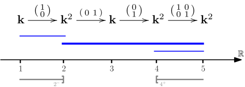
   Figure 1. A one-parameter persistence module $M$ (top) indexed over $\{1,2,3,4,5\}\subset{\mathbb{R}}$, and its barcode (in blue). The corresponding rank decomposition is $\operatorname{Rk}M=\operatorname{Rk}\mathbf{k}_{\llbracket 1,2\rrbracket}+\operatorname{Rk}\mathbf{k}_{\llbracket 2,5\rrbracket}+\operatorname{Rk}\mathbf{k}_{\llbracket 4,5\rrbracket}$. For instance, the rank $\operatorname{Rk}M(2,4)=1$ is given by the one bar (thickened) that connects the down-set $2^{-}$ to the up-set $4^{+}$.

3. Since the real line is totally ordered, all intervals in $\textnormal{Dgm}\,M$ are segments—possibly closed, open, or half-open. $\textnormal{Dgm}\,M$ can then be represented graphically as an actual barcode, whose bars are in bijective correspondence with the elements of $\textnormal{Dgm}\,M$—see Figure 1 for an illustration. This barcode reveals the global structure of the rank invariant $\operatorname{Rk}M$, and provides an interpretation for it, whereby each bar corresponds to the lifespan of some ‘persistent feature’. In particular, for any $s\leq t\in P$, the rank $\operatorname{Rk}M(s,t)$ is given by the number of bars that connect the down-set $s^{-}=\{u\in P\mid u\leq s\}$ to the up-set $t^{+}=\{u\in P\mid u\geq t\}$, i.e. the number of ‘features’ that persist between indices $s$ and $t$. Thus, $\textnormal{Dgm}\,M$ provides a visual tool for data exploration via the construction of one-parameter persistence modules.

4. Underlying (1.2) is a direct-sum decomposition of the module $M$ itself [15], more precisely:

   (1.3) $$M\simeq\bigoplus_{{I}\in\textnormal{Dgm}\,M}\mathbf{k}_{I}.$$

   This decomposition is also unique, as interval modules are indecomposable with local endomorphism ring. It grounds the rank decomposition (1.2) and its interpretation in algebra, whereby each ‘persistent feature’ corresponds to an actual summand of the module $M$. It also shows that $\textnormal{Dgm}\,M$ and $\operatorname{Rk}M$ are complete invariants of $M$.

5. When the poset $P$ is finite (or locally finite), say $P=\llbracket 1,n\rrbracket$, the barcode $\textnormal{Dgm}\,M$ is easily obtained from $\operatorname{Rk}M$ via the following inclusion-exclusion formula, where $\operatorname{mult}_{I}\textnormal{Dgm}\,M$ denotes the multiplicity of interval ${I}$ in the multi-set $\textnormal{Dgm}\,M$, and where by convention $\operatorname{Rk}M(0,j)=\operatorname{Rk}M(i,n+1)=0$ for all $1\leq i,j\leq n$:

   (1.4) $$\operatorname{mult}_{\llbracket i,j\rrbracket}\textnormal{Dgm}\,M=\operatorname{Rk}M(i,j)-\operatorname{Rk}M(i-1,j)-\operatorname{Rk}M(i,j+1)+\operatorname{Rk}M(i-1,j+1).$$

   In practice, when the module $M$ originates from some simplicial filtration, the persistence algorithm [18, 33] is able to compute $\textnormal{Dgm}\,M$ directly, without computing $M$ itself nor its rank invariant first.

6. Finally, the space of barcodes is naturally equipped with an optimal transportation metric, called the bottleneck distance, which makes it the isometric image of the space of one-parameter persistence modules equipped with its universal interleaving distance [12, 24]. A practical consequence of this isometry is that barcodes are stable with respect to perturbations of their originating data, and can therefore be used as compact descriptors for these data. In particular, vectorizations and kernels can be applied to turn these descriptors into stable feature vectors, to be plugged into machine learning pipelines.

This list of properties serves as a baseline to assess the relevance of any new invariant in the context of topological data analysis.

Unfortunately, some major difficulties arise when trying to generalize the concept of barcode to multi-parameter persistence modules—i.e. functors $M$ from ${\mathbb{R}}^{d}$ (viewed as a product of $d$ copies of the real line, equipped with the product order) to the vector spaces over $\mathbf{k}$. Foremost, while a direct-sum decomposition of $M$ into indecomposables still exists and is essentially unique [6], the summands may no longer be interval modules as in (1.3), where intervals in ${\mathbb{R}}^{d}$ are defined to be connected convex subsets in the product order.

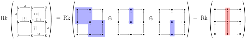
Figure 2. The indecomposable module $M$ on the left-hand side does not have the same rank invariant as any direct sum of interval modules on the $3\times 3$ grid. However, $\operatorname{Rk}M$ is equal to the difference between the rank invariants of two direct sums of interval modules, as shown on the right-hand side. Blue is for intervals counted positively in the decomposition, while red is for intervals counted negatively.

For instance, the module on the left-hand side of Figure 2 is indecomposable yet not an interval module nor even an indicator module—its pointwise dimension is not everywhere $\leq 1$. One may then ask whether rank decompositions such as (1.2) exist nonetheless. This is a reasonable question since the rank invariant is known to be incomplete on multi-parameter persistence modules. The answer turns out to be negative though: still in Figure 2, the module $M$ on the left-hand side does not have the same rank invariant as any direct sum of interval modules, therefore it cannot decompose as in (1.2). Nevertheless, $\operatorname{Rk}M$ can be expressed as the difference between the rank invariants of two direct sums of interval modules, as illustrated in the figure. In other words, $\operatorname{Rk}M$ decomposes as a ${\mathbb{Z}}$-linear combination of rank invariants of interval modules, with possibly negative coefficients. This suggests that the proper generalization of the rank decomposition (1.2) to multi-parameter persistence should be a signed rank decomposition, which will be our main object of study.

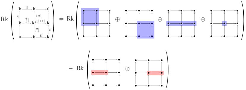
Figure 3. Minimal rank decomposition of the rank invariant of the module $M$ from Figure 2 over the collection of rectangles in the $3\times 3$ grid. Blue is for rectangles in $\mathcal{R}$, while red is for rectangles in $\mathcal{S}$.

Figure 3 shows another possible signed rank decomposition for the module $M$ of Figure 2, illustrating the fact that such decompositions may not always be unique. Uniqueness is important in the context of topological data analysis, where users ultimately want a reliable interpretation of the structure of the persistence module—or its rank invariant—from its decomposition. For this, the choice of the collection of intervals over which to decompose the rank invariant is paramount: the smaller the collection, the bigger chances decompositions have to be unique, but at the same time the smaller chances they have to exist. Meanwhile, the simpler the shapes in the collection of intervals, the more straightforward the interpretation of the decomposition. For instance, the module $M$ of Figure 2 admits essentially one rank decomposition involving only rectangles, shown in Figure 3. Uniqueness in this case mainly comes from the known fact that the rank invariant is complete on direct sums of rectangle modules, i.e. interval modules supported on rectangles [7, 20]. Finding the right conditions under which signed rank decompositions involving rectangles (or some richer but fixed class of shapes) are uniquely defined will be our first main objective.

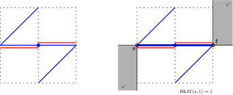
Figure 4. Left: the signed barcode corresponding to the rank decomposition of Figure 3. Each bar is the diagonal with positive slope of one of the rectangles involved in the decomposition, with the same color code (blue for positive sign, red for negative sign). Right: computing $\operatorname{Rk}M(s,t)$ for a pair of indices $s\leq t$ (the thick bar is the only one connecting the down-set $s^{-}$ to the up-set $t^{+}$).

Rectangles are a particularly interesting type of shapes for us because they are the simplest intervals in ${\mathbb{R}}^{d}$, entirely determined by their upper bound and lower bound. They allow for an alternative representation of the signed rank decomposition as a signed barcode, where each bar is the diagonal (with positive slope) of a particular rectangle in the decomposition, with the same sign—see Figure 4 (left) for an illustration. The signed barcode encodes visually the global structure of the rank invariant, and it gives access to the same information as the signed rank decomposition. For instance, the rank $\operatorname{Rk}M(s,t)$ between a pair of indices $s\leq t$ is given by the number of positive bars that connect the down-set $s^{-}=\{u\in P\mid u\leq s\}$ to the up-set $t^{+}=\{u\in P\mid u\geq t\}$, minus the number of negative bars that connect $s^{-}$ to $t^{+}$—see Figure 4 (right). This is exactly the same thing as with barcodes in the one-parameter case, except the contribution of each bar to the rank is now signed. Understanding how the signed barcodes can be leveraged in applications, and potentially extended to larger classes of shapes than rectangles, will be our second main objective.

Our third main objective will be to ground the signed decompositions in algebra, like their unsigned counterparts in one-parameter persistence. Since the rank invariant is no longer complete, and direct-sum decompositions of the modules may not contain only interval summands, it sounds unreasonable to try to connect the two together. However, the fact that rank decompositions may now contain negative terms gives us a hint that they might be connected to certain kinds of resolutions of the modules.

1.2. Our setting

We work more generally over a partially ordered set $P$, considered as a category in the obvious way, and we let $\mathbf{k}$ be an arbitrary but fixed field. Closed rectangles in ${\mathbb{R}}^{d}$ now become closed segments in $P$, defined by $\langle s,t\rangle=\{u\in P\mid s\leq u\leq t\}$. Intervals in $P$ are defined as non-empty subsets ${I}$ that are both convex and connected in the partial order:

• if $s\leq u\leq t$ and $s,t\in{I}$, then $u\in{I}$;

• if $s,t\in{I}$, then there are $u_{0},\ldots,u_{n+1}\in{I}$ such that $u_{i}$ and $u_{i+1}$ are comparable for all $0\leq i\leq n$ and $u_{0}=s$ and $u_{n+1}=t$.

Denote by $\operatorname{Rep}P$ the functor category consisting of all functors $M\colon P\to\mathrm{Vec}_{\mathbf{k}}$ where $\mathrm{Vec}_{\mathbf{k}}$ is the category of vector spaces over $\mathbf{k}$. We shall refer to such a functor $M$ either as a representation of $P$ or as a persistence module over $P$, without distinction. Let $\operatorname{rep}P$ be the subcategory of pointwise finite-dimensional (pfd) representations, i.e. functors taking their values in the finite-dimensional vector spaces over $\mathbf{k}$. Denoting by

$$\{{\leq}_{P}\}=\{(a,b)\in P\times P\mid a\leq b\}$$

the set of pairs defining the partial order in $P$, we see the rank invariant (1.1) as a map $\{{\leq}_{P}\}\to{\mathbb{N}}$ (in the literature, the rank invariant is sometimes defined as a map on $P\times P$ that vanishes outside $\{{\leq}_{P}\}$; such a map clearly holds the same information as our rank invariant).

Since the usual rank invariant is incomplete, even on the subcategory of interval-decomposable modules (i.e. modules isomorphic to direct sums of interval modules), we will consider a generalization of the rank invariant that probes the existence of ‘features’ in the module across arbitrary intervals ${I}\subseteq P$, not just across closed segments. This generalization is known to be complete on interval-decomposable modules—see [20] or our Proposition 2.10:

Definition 1.1.

Let $M\in\operatorname{Rep}P$. Given an interval ${I}\subseteq P$, the generalized rank of $M$ over ${I}$, denoted by $\operatorname{Rk}_{I}M$, is defined by:

$$\operatorname{Rk}_{I}M=\operatorname{rank}\left[\varprojlim M|_{I}\to\varinjlim M|_{I}\right].$$

Given a collection $\mathcal{I}$ of intervals, the generalized rank invariant of $M$ over $\mathcal{I}$ is the map $\operatorname{Rk}_{\mathcal{I}}M\colon\mathcal{I}\to{\mathbb{N}}\cup\{\infty\}$ defined by $\operatorname{Rk}_{\mathcal{I}}M({I})=\operatorname{Rk}_{I}M$.

Note that the morphism $\varprojlim M|_{I}\to\varinjlim M|_{I}$ in the above definition is well-defined because intervals are both convex and connected. In this paper we are only interested in generalized rank invariants that are finite, i.e. that take only finite values. We write $\operatorname{rep}_{\mathcal{I}}P$ for the subcategory of representations that have a finite generalized rank invariant over $\mathcal{I}$.

Remark 1.2.

If $M\in\operatorname{rep}P$ then $\operatorname{rank}\left[\varprojlim M|_{I}\to\varinjlim M|_{I}\right]$ is finite for any interval ${I}$, because the morphism factors through the internal spaces of $M|_{I}$, which are finite-dimensional. Thus, we always have $\operatorname{rep}P\subseteq\operatorname{rep}_{\mathcal{I}}P$, and the inclusion is an equality precisely when $\mathcal{I}$ contains all singletons.

Remark 1.3.

To see that Definition 1.1 generalizes the standard rank invariant, observe that when ${I}$ is a closed segment $\langle i,j\rangle=\{u\in P\mid i\leq u\leq j\}$, we have $\operatorname{Rk}_{I}M=\operatorname{rank}\left[M(i)\to M(j)\right]$. Hence, taking $\mathcal{I}=\{\langle i,j\rangle\mid i\leq j\in P\}\simeq\{{\leq}_{P}\}$ in the above definition gives $\operatorname{Rk}_{\mathcal{I}}M=\operatorname{Rk}M$, the usual rank invariant of $M$.

Our most general setting considers signed rank decompositions of arbitrary maps $\mathcal{I}\to{\mathbb{Z}}$, not just of finite generalized rank invariants. This way, our existence and uniqueness results may find applications beyond multi-parameter persistence and poset representations. From now on, we merely talk about rank decompositions, making implicit the fact that they are signed—which is obvious from the context.

Definition 1.4.

Given a collection $\mathcal{I}$ of intervals in $P$, and a function $r\colon\mathcal{I}\to\mathbb{Z}$, a (signed) rank decomposition of $r$ over $\mathcal{I}$ is given by the following kind of identity:

$$r=\operatorname{Rk}_{\mathcal{I}}\mathbf{k}_{\mathcal{R}}-\operatorname{Rk}_{\mathcal{I}}\mathbf{k}_{\mathcal{S}},$$

where $\mathcal{R}$ and $\mathcal{S}$ are multi-sets of elements taken from $\mathcal{I}$ such that $\mathbf{k}_{\mathcal{R}}$ and $\mathbf{k}_{\mathcal{S}}$ lie in $\operatorname{rep}_{\mathcal{I}}P$, and where by definition $\mathbf{k}_{\mathcal{R}}=\bigoplus_{{R}\in\mathcal{R}}\mathbf{k}_{R}$ and $\mathbf{k}_{\mathcal{S}}=\bigoplus_{{S}\in\mathcal{S}}\mathbf{k}_{S}$ (note that elements ${R}\in\mathcal{R}$ and ${S}\in\mathcal{S}$ are considered with multiplicity in the direct sums). By extension, we call the pair $(\mathcal{R},\mathcal{S})$ itself a rank decomposition of $r$ over $\mathcal{I}$. It is a minimal rank decomposition if $\mathcal{R}$ and $\mathcal{S}$ are disjoint as multi-sets.

Note that $\operatorname{Rk}_{\mathcal{I}}\mathbf{k}_{R}({I})=\mathds{1}_{{R}\supseteq{I}}$ for any ${I}\in\mathcal{I}$ and ${R}\in\mathcal{R}$ (Proposition 2.1), so $\operatorname{Rk}_{\mathcal{I}}\mathbf{k}_{\mathcal{R}}({I})=\operatorname{Rk}_{I}\mathbf{k}_{\mathcal{R}}$ actually counts the number of elements in $\mathcal{R}$ that span the interval ${I}$. This number is required to be finite for every ${I}\in\mathcal{I}$ in the definition, so that $\mathbf{k}_{\mathcal{R}}\in\operatorname{rep}_{\mathcal{I}}P$; by Remark 1.2, a sufficient condition for this is that $\mathbf{k}_{\mathcal{R}}\in\operatorname{rep}P$, which means that $\mathcal{R}$ is pointwise finite, i.e. that only finitely many elements of $\mathcal{R}$ cover any given index in $P$; it is also a necessary condition when $\mathcal{I}$ contains all the singletons in $P$.

An important consequence of having $\operatorname{Rk}_{\mathcal{I}}\mathbf{k}_{R}({I})=\mathds{1}_{{R}\supseteq{I}}$ is that adding the same number of copies of an interval ${I}\in\mathcal{I}$ to both $\mathcal{R}$ and $\mathcal{S}$ does not change the difference $\operatorname{Rk}_{\mathcal{I}}\mathbf{k}_{\mathcal{R}}-\operatorname{Rk}_{\mathcal{I}}\mathbf{k}_{\mathcal{S}}$, so rank decompositions cannot be unique. This motivates the introduction of minimal rank decompositions, which further require the multi-sets $\mathcal{R},\mathcal{S}$ to be disjoint, and thus can be proven to be unique.

Let us emphasize the importance of asking the intervals involved in the rank decompositions of $r\colon\mathcal{I}\to{\mathbb{Z}}$ to be taken from $\mathcal{I}$, and not from outside of $\mathcal{I}$, in Definition 1.4. This condition is to ensure the uniqueness and interpretability of the minimal rank decomposition of $r$. For instance, Figures 2 and 3 show two different minimal decompositions of the usual rank invariant of the same module $M$, but only the one from Figure 3 is valid as per Definition 1.4. The other one involves an interval ${I}$ that is not a rectangle in the $3\times 3$ grid, while $\operatorname{Rk}M$ is a ${\mathbb{Z}}$-valued map defined only on the rectangles (see Remark 1.3); it leads to the wrong interpretation that some ‘persistent feature’ spans the entire non-rectangle interval ${I}$, whereas no such feature exists in the module $M$, whose generalized rank over ${I}$ is zero. See Section 8 for further discussion on this topic.

1.3. Our contributions

Our results are best viewed in light of the properties (a)-(f) of one-parameter persistence barcodes listed in Section 1.1. Each individual property turns out to be satisfied either fully or in part by our more general minimal rank decompositions in the multi-parameter setting.

In Section 2 we study the existence and uniqueness of minimal rank decompositions. We show in Theorem 2.11 and Corollary 2.12 that a minimal rank decomposition $(\mathcal{R},\mathcal{S})$ of a given map $r:\mathcal{I}\to{\mathbb{Z}}$ exists as soon as rank decompositions of $r$ themselves exist, that it is always unique, and that it satisfies the following universality property justifying its name: for any other rank decomposition $(\mathcal{R}^{\prime},\mathcal{S}^{\prime})$ of $r$ over $\mathcal{I}$, we have $\mathcal{R}^{\prime}\supseteq\mathcal{R}$, $\mathcal{S}^{\prime}\supseteq\mathcal{S}$, and $\mathcal{R}^{\prime}\setminus\mathcal{R}=\mathcal{S}^{\prime}\setminus\mathcal{S}$. To complete the picture, in Corollary 2.6 we prove the existence of rank decompositions in the first place, under the mild condition that the collection $\mathcal{I}$ of intervals under consideration is locally finite, and that the maps $r:\mathcal{I}\to{\mathbb{Z}}$ considered have locally finite support—see Section 2 for proper definitions. Our proof emphasizes the role played by the family of generalized rank invariants $(\operatorname{Rk}_{\mathcal{I}}\mathbf{k}_{I})_{{I}\in\mathcal{I}}$, which acts as a generalized basis (Theorem 2.5). These results imply that the minimal rank decompositions satisfy properties (a) and (b) from Section 1.1.

In Section 3 we focus on the computation of the coefficients in the minimal rank decompositions. For this purpose we connect minimal rank decompositions to the so-called generalized persistence diagrams [28], and we derive an explicit inclusion-exclusion formula (Corollary 3.5) that corresponds to taking the Möbius inverse of the generalized rank invariant (Proposition 3.3). This satisfies property (e) from Section 1.1.

In Section 4 we ground the rank decompositions in algebra, by showing how they derive from projective resolutions in a certain exact category, thus satisfying property (d) from Section 1.1. More precisely, we define an exact structure on the category of pfd representations of $P$ by considering exact sequences that preserve ranks. Such exact sequences are called rank-exact, and the corresponding exact structure is called the rank-exact structure. Then, we show how the interval-decomposable representations $\mathbf{k}_{\mathcal{R}}$ and $\mathbf{k}_{\mathcal{S}}$ involved in the rank decompositions are connected to each other via short rank-exact sequences (Theorem 4.10). This formulation allows us to derive existence results for rank decompositions of finitely presented representations of posets that may not be locally finite (Theorem 4.16).

In Section 5 we reformulate our results in the specific context of multi-parameter persistence. We thus obtain existence and uniqueness results for minimal rank decompositions of finitely presented persistence modules over ${\mathbb{R}}^{d}$, and of pfd persistence modules over finite grids. In the latter case, we also derive an explicit inclusion-exclusion formula to compute the coefficients in the minimal rank decompositions. This formula matches with (1.4) in the one-parameter case, and with the formula derived in [7] for the usual rank invariant in the 2-parameter case. Finally, we discuss the stability of the minimal rank decompositions and propose a metric in which to compare them, based on the matching (pseudo-)distance from [22]. In this metric we show that the minimal rank decompositions are the ones maximizing the distance (Proposition 5.10), and that replacing the modules by their rank decompositions does not expand their pairwise distances (Theorem 5.9), thus satisfying in part property (f) from Section 1.1.

In Section 6 we introduce the signed barcode as a visual representation of the minimal rank decomposition of the usual rank invariant. We explain how the signed barcode reflects the global structure of the usual rank invariant, and how its role in multi-parameter persistence is similar to the one played by the unsigned barcode in one-parameter persistence. We also discuss its extension to generalized rank invariants, for which it takes the form of a ‘decorated’ signed barcode with similar properties and extra information. This satisfies property (c) from Section 1.1.

In Section 7 we carry out a round of experiments, whose outcomes illustrate some of the key properties of the minimal rank decompositions and of their associated signed barcodes.

Finally, in Section 8 we conclude the paper with a detailed discussion on the perspectives open by this work, and on the inherent limitations of rank decompositions.

1.4. Related work

Our work has deep connections to the line of work on generalized persistence diagrams, first initiated by Patel [28]. Patel pointed out that the inclusion-exclusion formula (1.4) corresponds to taking the Möbius inverse of the rank invariant, and can therefore be used to define generalized persistence diagrams for 1-parameter persistence modules valued in certain symmetric monoidal categories beyond $\mathrm{Vec}_{\mathbf{k}}$. In a different context, Betthauser et al. [4] defined the related concept of graded persistence diagram, obtained by taking the Möbius inverse of the unary representation of the rank function of a 1-parameter persistence module. They proved a Wasserstein stability theorem for graded persistence diagrams, and connected them to persistence landscapes.

McCleary and Patel [26] extended the concept of generalized persistence diagram to the multi-parameter setting, more precisely to persistence modules indexed over finite metric lattices, replacing the usual rank invariant by the equivalent birth-death function in the Möbius inversion. They built a functorial pipeline, and they proved that it is stable in the edit distance.

Kim and Mémoli [20] extended the concept further, to persistence modules indexed over posets that are essentially finite, and for this they used the natural order on intervals given by inclusion. Their generalized persistence diagram is defined as the Möbius inverse of the generalized rank invariant over the full collection $\mathcal{I}$ of intervals in the poset. It may have negative coefficients, and it is not proven to be stable, however it is proven to be a complete invariant on the subcategory of interval-decomposable modules, encoding the multiplicities of the summands in the direct-sum decomposition of such modules.

Asashiba et al. [2] proceed essentially in the same way, and they arrive at similar conclusions, albeit using a different language. Despite the fact that their focus is limited to the two-parameter setting, their viewpoint is interesting in that they present the generalized persistence diagram of a module $M$ as some kind of rank-preserving ‘projection’ of $M$ onto the ‘signed’ direct sums of interval modules (defined mathematically as elements of the split Grothendieck group of $\operatorname{Rep}P$), which in essence is very close to what our minimal rank decompositions are.

Here we put the generalized persistence diagrams in the larger context of rank decompositions. Our results show the existence of such decompositions, not only for the usual rank invariant or for the generalized rank invariant over the full collection of intervals in the poset, but also for the generalized rank invariant over arbitrary subcollections $\mathcal{I}$ of intervals. We show that the generalized persistence diagrams, whenever they exist (i.e. when Möbius inversions are defined), actually correspond to the minimal rank decompositions, which we prove to be unique and to satisfy a certain universality property. Our framework allows us to prove these results using fairly direct arguments that (1) emphasize the role played by the family of rank invariants of interval modules as a generalized basis for the space of maps $\mathcal{I}\to{\mathbb{Z}}$, and (2) hold over more general classes of posets in which Möbius inversions may no longer be defined. Meanwhile, it connects the rank decompositions to projective resolutions of the modules in a certain exact structure, in a similar way as persistence diagrams are connected to direct-sum decompositions in the one-parameter setting. It also allows us to derive new stability results, in terms of the matching distance $\mathrm{d}_{\mathrm{match}}$ from [22], which is a natural choice of distance as far as rank invariants are concerned. Finally, it allows us to introduce the signed barcodes as a practical graphical representation for minimal rank decompositions, and so for generalized persistence diagrams as well.

To understand the significance of our contribution, it is important to bear in mind that Möbius inversion is but one of many possible invertible operators (including the identity operator) that can be applied to the rank invariant or its generalized version. Prior to this work, choosing Möbius inversion over any other invertible operator was mainly motivated by an analogy with the 1-parameter setting, without further mathematical grounding akin to the decomposition theorem for 1-parameter persistence modules. Here we provide such grounding at two different levels:

• at the functional level, we show that taking the Möbius inverse of the (usual or generalized) rank invariant corresponds to decomposing the invariant over a basis, composed of the rank invariants of certain classes of interval modules;

• at the algebraic level, we connect usual rank decompositions to projective resolutions in the rank-exact structure, the latter being induced precisely by those exact sequences that preserve the rank invariant.

To complete the picture, let us mention that our work opens up a line of research on defining new invariants for persistence modules using exact structures, in order to encode the modules in terms of segments and intervals. Blanchette, Brüstle, and Hanson [5] are also investigating this direction, and they recently proved the finiteness of the global dimension of certain exact structures on finite posets, including our rank-exact structure, thus extending our Theorem 4.8.

Acknowledgements

The authors wish to thank Luis Scoccola for raising the question of discriminating the signal from the noise in signed barcodes, and for suggesting the signed prominence diagram as a representation of the barcode for this purpose. His comments and feedback have eventually led to the development of Section 6.3 of this paper.

2. Rank Decompositions: Existence and Uniqueness

In Section 2.1 (Corollary 2.6) we show that every map $r\colon\mathcal{I}\to{\mathbb{Z}}$ with locally finite support admits a unique minimal rank decomposition, provided the underlying collection of intervals $\mathcal{I}$ itself is locally finite—precise definitions of local finiteness are provided in the section. Then, in Section 2.2 we drop all previous assumptions and work with arbitrary maps $r$ over arbitrary collections of intervals $\mathcal{I}$ in an arbitrary poset $P$. In this general setting, we show that minimal rank decompositions still exist and are still unique as long as rank decompositions themselves exist (Corollary 2.12). Finally, in Section 2.3 we study how rank decompositions behave under restrictions to subposets of $P$ (Proposition 2.16).

The following proposition, which generalizes [20, Proposition 3.17] by dropping the assumption of local finiteness of the poset $P$ and allowing for generalized ranks, and which is given a more direct proof, will be instrumental throughout our analysis.

Proposition 2.1.

Let $\mathcal{R}$ be a multi-set of intervals of $P$. Then, for any interval ${I}\subseteq P$, we have:

$$\operatorname{Rk}_{I}(\mathbf{k}_{\mathcal{R}})=\#\{{R}\in\mathcal{R}\mid{I}\subseteq{R}\}.$$

Proof.

Note that

$$\mathbf{k}_{\mathcal{R}}|_{{I}}=\bigoplus_{{R}\in\mathcal{R}}\mathbf{k}_{{R}\cap{I}}=\bigoplus_{\begin{subarray}{c}{R}\in\mathcal{R}\\ {I}\subseteq{R}\end{subarray}}\mathbf{k}_{{I}}\oplus\bigoplus_{{R}\in\widetilde{\mathcal{R}}}\mathbf{k}_{{R}},$$

where $\widetilde{\mathcal{R}}$ is a collection of proper subintervals of ${I}$. (Note that while the ${R}\cap{I}$ are not necessarily connected themselves, they are disjoint unions of intervals.)

Since the rank commutes with finite sums, and clearly $\operatorname{Rk}_{{I}}(\bigoplus_{\begin{subarray}{c}{R}\in\mathcal{R}\\ {I}\subseteq{R}\end{subarray}}\mathbf{k}_{{I}})=\#\{{R}\in\mathcal{R}\mid{I}\subseteq{R}\}$, it suffices to show that $\operatorname{Rk}_{{I}}(\bigoplus_{{R}\in\widetilde{\mathcal{R}}}\mathbf{k}_{{R}})=0$ for any multi-set $\widetilde{\mathcal{R}}$ of proper subintervals of ${I}$.

Our next step is to note that for any such proper subinterval ${R}$ of ${I}$ at least one of $\varprojlim\mathbf{k}_{{R}}|_{{I}}$ or $\varinjlim\mathbf{k}_{{R}}|_{{I}}$ is zero: indeed, we may observe that $\varprojlim\mathbf{k}_{{R}}|_{{I}}$ is non-zero precisely if ${R}$ is closed under predecessors in ${I}$. Dually, $\varinjlim\mathbf{k}_{{R}}|_{{I}}\neq 0$ precisely if ${R}$ is closed under successors in ${I}$. Since a proper subinterval cannot be closed both under predecessors and successors, it follows that at least one of limit or colimit is zero.

Going back to our multi-set $\widetilde{\mathcal{R}}$ of proper subintervals of ${I}$, we can now decompose it as $\widetilde{\mathcal{R}}=\mathcal{R}^{\prime}\cup\mathcal{R}^{\prime\prime}$ where $\mathcal{R}^{\prime}$ only contains subintervals ${R}\subsetneq{I}$ with $\varprojlim_{I}\mathbf{k}_{{R}}=0$, and $\mathcal{R}^{\prime\prime}$ only contains subintervals ${R}\subsetneq{I}$ with $\varinjlim_{{I}}\mathbf{k}_{{R}}=0$. (This decomposition will typically not be unique, as there may be subintervals for which both limit and colimit vanish.) Again invoking the fact that rank commutes with finite sums, it suffices to show that $\operatorname{Rk}_{{I}}(\mathbf{k}_{\mathcal{R}^{\prime}})=0$ and $\operatorname{Rk}_{{I}}(\mathbf{k}_{\mathcal{R}^{\prime\prime}})=0$.

The latter is immediate, since direct sums commute with colimits, and hence $\varinjlim_{{I}}\mathbf{k}_{\mathcal{R}^{\prime\prime}}=0$. For the former, we additionally use that the direct sum is naturally a subrepresentation of the direct product, and moreover that limits are left exact. This gives us

$$\varprojlim_{{I}}\mathbf{k}_{\mathcal{R}^{\prime}}\subseteq\varprojlim_{{I}}\prod_{{R}\in\mathcal{R}^{\prime}}\mathbf{k}_{{R}}=\prod_{{R}\in\mathcal{R}^{\prime}}\varprojlim_{{I}}\mathbf{k}_{{R}}=0.\qed$$

Remark 2.2.

One might hope that an analogous result holds if one replaced the sum in the definition of $\mathbf{k}_{\mathcal{R}}$ by a product. However, the following example shows this to not be the case:

Let ${I}=\{(x,y)\in\mathbb{R}^{2}\mid x\geq 0,y\geq 0,x+y\leq 1\}$, and pick an infinite set $\{p_{s}\mid s\in S\}$ of pairwise different maximal points in ${I}$. Let ${R}_{s}={I}\setminus\{p_{s}\}$. Then

$$\operatorname{Rk}_{{I}}\left(\prod_{s\in S}\mathbf{k}_{{R}_{s}}\right)=\infty.$$

(The key point here is that $\varinjlim_{{I}}\prod_{s\in S}\mathbf{k}_{{R}_{s}}=\mathbf{k}^{S}/\mathbf{k}^{(S)}\neq 0$.)

Corollary 2.3.

Let $\mathcal{I}$ be a collection of intervals in $P$. For a multi-set $\mathcal{R}$ of intervals, we have that $\mathbf{k}_{\mathcal{R}}\in\operatorname{rep}_{\mathcal{I}}P$ if and only if

$$\forall{I}\in\mathcal{I},\quad\#\{{R}\in\mathcal{R}\mid{I}\subseteq{R}\}<\infty.$$

2.1. The locally finite case

Let $\mathcal{I}$ be a locally finite collection of intervals in $P$. That is, for any two comparable intervals in $\mathcal{I}$, there are only finitely many intervals in $\mathcal{I}$ between the two. We say a map $\mathcal{I}\to{\mathbb{Z}}$ has locally finite support if its restriction to the up-set of any element of $\mathcal{I}$ has finite support.

Remark 2.4.

For any fixed ${I}\in\mathcal{I}$, the map $\operatorname{Rk}_{\mathcal{I}}\mathbf{k}_{I}\colon{J}\mapsto\operatorname{Rk}_{{J}}\mathbf{k}_{{I}}$ has locally finite support, by the description in Proposition 2.1. More generally, for any multi-set $\mathcal{R}$ of elements in $\mathcal{I}$, if $\mathbf{k}_{\mathcal{R}}\in\operatorname{rep}_{\mathcal{I}}P$ then the map $\operatorname{Rk}_{\mathcal{I}}\mathbf{k}_{\mathcal{R}}$ has locally finite support: for any fixed ${I}\in\mathcal{I}$, by Corollary 2.3 $\mathcal{R}$ only contains finitely many elements containing ${I}$, and these are the only ones relevant when considering the restriction of $\operatorname{Rk}_{\mathcal{I}}\mathbf{k}_{\mathcal{R}}$ to the up-set of ${I}$.

Theorem 2.5.

Let $\mathcal{I}$ be a locally finite collection of intervals in $P$. Then any function $r\colon\mathcal{I}\to{\mathbb{Z}}$ with locally finite support can uniquely be written as a (possibly infinite, but pointwise finite) ${\mathbb{Z}}$-linear combination of the functions $\operatorname{Rk}_{\mathcal{I}}\mathbf{k}_{{I}}$ with ${I}\in\mathcal{I}$.

Proof.

Existence: For any ${I}\in\mathcal{I}$ we set $S_{{I}}=\{{J}\supseteq{I}\mid\exists{K}\supseteq{J}\text{ with }r({K})\neq 0\}$. Since $r$ is locally finite, its support restricted to the up-set of ${I}$ is finite, and so is $S_{{I}}$ since $\mathcal{I}$ is locally finite.

Now we define a collection of scalars $\alpha_{{I}}\in{\mathbb{Z}}$ for ${I}\in\mathcal{I}$, inductively on the size of $S_{{I}}$: If $S_{{I}}=\varnothing$ we set $\alpha_{{I}}=0$. Otherwise we set

$$\alpha_{{I}}=r({I})-\sum_{{J}\in S_{{I}}\setminus\{{I}\}}\alpha_{{J}}.$$

Note that for ${J}\in S_{{I}}\setminus\{{I}\}$ we have $S_{{J}}\subsetneq S_{{I}}$, so the terms on the right hand side are already defined.

Now, using the description of the map $\operatorname{Rk}_{\mathcal{I}}\mathbf{k}_{{I}}$ in Proposition 2.1, one immediately verifies that $r=\sum_{{I}\in\mathcal{I}}\alpha_{{I}}\operatorname{Rk}_{\mathcal{I}}\mathbf{k}_{{I}}$. (Note in particular that this infinite sum is pointwise finite — on a given interval ${J}$ the only possibly non-zero terms are the ones in $S_{{J}}$ —hence well-defined.)

Uniqueness: subtracting two different ${\mathbb{Z}}$-linear combinations realizing $r$ from each other, we get a single linear combination $\sum_{{I}\in\mathcal{I}}\alpha_{{I}}\operatorname{Rk}_{\mathcal{I}}\mathbf{k}_{{I}}$ with non-zero coefficients which sums up to zero. Note that there is at least one maximal ${I}\in\mathcal{I}$ such that $\alpha_{{I}}\neq 0$, for otherwise the sum would not be defined. It follows, again using Proposition 2.1, that $(\sum_{{J}\in\mathcal{I}}\alpha_{{J}}\operatorname{Rk}_{\mathcal{I}}\mathbf{k}_{{J}})({I})=\alpha_{{I}}\neq 0$, contradicting our assumption. ∎

Corollary 2.6.

Let $\mathcal{I}$ be a locally finite collection of intervals in $P$. Then, for any map $r\colon\mathcal{I}\to{\mathbb{Z}}$ with locally finite support, there is a unique pair $\mathcal{R},\mathcal{S}$ of disjoint multi-sets of elements of $\mathcal{I}$ such that $\mathbf{k}_{\mathcal{R}}$ and $\mathbf{k}_{\mathcal{S}}$ lie in $\operatorname{rep}_{\mathcal{I}}P$ and satisfy the following identity:

$$r=\operatorname{Rk}_{\mathcal{I}}\mathbf{k}_{\mathcal{R}}-\operatorname{Rk}_{\mathcal{I}}\mathbf{k}_{\mathcal{S}}.$$

Proof.

By Theorem 2.5, there is a unique (possibly infinite, but pointwise finite) ${\mathbb{Z}}$-linear combination of functions $r=\sum_{{I}\in\mathcal{I}}\alpha_{{I}}\,\operatorname{Rk}_{\mathcal{I}}\mathbf{k}_{{I}}$. Let then $\mathcal{R}=\{{I}\in\mathcal{I}\mid\alpha_{{I}}>0\}$ with multiplicities ${I}\mapsto\alpha_{{I}}$, and $\mathcal{S}=\{{I}\in\mathcal{I}\mid\alpha_{{I}}<0\}$ with multiplicities ${I}\mapsto|\alpha_{{I}}|$. It follows from the pointwise-finiteness of the linear combination that $\mathcal{R}$ and $\mathcal{S}$ satisfy the condition in Corollary 2.3, so in particular $\mathbf{k}_{\mathcal{R}}$ and $\mathbf{k}_{\mathcal{S}}$ lie in $\operatorname{rep}_{\mathcal{I}}P$. ∎

Specializing Theorem 2.5 and Corollary 2.6 to the case where $P$ is finite and $\mathcal{I}=\{\langle i,j\rangle\mid i\leq j\in P\}\simeq\{{\leq}_{P}\}$ yields the following results—where $\operatorname{Rk}_{\mathcal{I}}$ becomes the usual rank invariant $\operatorname{Rk}$ according to Remark 1.3:

Corollary 2.7.

Let $P$ be a finite poset. Then the collection of maps $\operatorname{Rk}\mathbf{k}_{\langle a,b\rangle}$ with $a\leq b$ is a basis of ${\mathbb{Z}}^{\{{\leq}_{P}\}}$.

Corollary 2.8.

Given a finite poset $P$, for any map $r:\{{\leq}_{P}\}\to{\mathbb{Z}}$ there is a unique pair $\mathcal{R},\mathcal{S}$ of disjoint finite multi-sets of closed segments such that

$$r=\operatorname{Rk}\mathbf{k}_{\mathcal{R}}-\operatorname{Rk}\mathbf{k}_{\mathcal{S}}.$$

Remark 2.9.

As mentioned in the general introduction of the paper, the interest of these results goes beyond the setting of persistence modules. For instance, when $P=\llbracket 1,n\rrbracket$ and $\mathcal{I}=\{\langle i,j\rangle\mid 1\leq i\leq j\leq n\}$, the space ${\mathbb{Z}}^{\mathcal{I}}$ is isomorphic to the space of symmetric $n\times n$ matrices with coefficients in ${\mathbb{Z}}$. In this setting, Theorem 2.5 says that every such matrix decomposes uniquely as a finite ${\mathbb{Z}}$-linear combination of binary matrices $M_{ab}$ supported each on a single diagonal block $\{(i,j)\mid a\leq i,j\leq b\}$. Indeed, each matrix $M_{ab}$ encodes (after symmetrization) the usual rank invariant of the indecomposable $\mathbf{k}_{\langle a,b\rangle}$.

2.2. The general case

We now drop our previous finiteness assumptions and consider arbitrary maps $r:\mathcal{I}\to{\mathbb{Z}}$ over an arbitrary collection $\mathcal{I}$ of intervals in an arbitrary poset $P$. Our first result shows that $\operatorname{Rk}_{\mathcal{I}}$ is a complete invariant when restricted to interval-decomposable representations supported on intervals in $\mathcal{I}$. In fact, we show that the rank invariant is complete on a slightly larger collection of intervals. This generalizes [20, Theorem 3.14].

Proposition 2.10.

Let $\mathcal{I}$ denote a collection of intervals in $P$, and let $\widehat{\mathcal{I}}\supseteq\mathcal{I}$ be the collection of limit intervals (which by construction are also intervals, i.e. non-empty connected convex subsets of $P$):

$$\widehat{\mathcal{I}}:=\left\{\bigcup_{x\in X}{I}_{x}\mid X\text{ totally ordered},{I}_{x}\in\mathcal{I}\ \mbox{and}\ {I}_{x}\subseteq{I}_{y}\ \forall x\leq y\in X\right\}.$$

If $\mathcal{R}$ and $\mathcal{R}^{\prime}$ are two multi-sets of elements in $\widehat{\mathcal{I}}$, such that $\operatorname{Rk}_{\mathcal{I}}\mathbf{k}_{\mathcal{R}}=\operatorname{Rk}_{\mathcal{I}}\mathbf{k}_{\mathcal{R}^{\prime}}$ and this common rank invariant is finite, then $\mathcal{R}=\mathcal{R}^{\prime}$.

Proof.

Since the rank of a direct sum is the sum of the ranks we may remove the common elements from $\mathcal{R}$ and $\mathcal{R}^{\prime}$, and thus assume that the two multi-sets are disjoint. It follows from the description of multi-sets giving rise to finite ranks in Corollary 2.3 that $\mathcal{R}\cup\mathcal{R}^{\prime}$ contains at least one maximal element, say ${J}$. Without loss of generality we assume ${J}\in\mathcal{R}$. By definition of $\widehat{\mathcal{I}}$ we have ${J}=\bigcup_{x\in X}{J}_{x}$ with ${J}_{x}\in\mathcal{I}$ and ${J}_{x}\subseteq{J}_{y}$ for all $x\leq y\in X$. Now, by assumption, for every $x\in X$ we have

$$\operatorname{Rk}_{{J}_{x}}\mathbf{k}_{\mathcal{R}^{\prime}}=\operatorname{Rk}_{{J}_{x}}\mathbf{k}_{\mathcal{R}}\geq\operatorname{Rk}_{{J}_{x}}\mathbf{k}_{{J}},$$

which is at least $1$ by Proposition 2.1. It also follows from Proposition 2.1 that, for each $x\in X$, there is some interval ${I}_{x}\in\mathcal{R}^{\prime}$ such that ${J}_{x}\subseteq{I}_{x}$. Since $\operatorname{Rk}_{\mathcal{I}}\mathbf{k}_{\mathcal{R}^{\prime}}$ is finite, Corollary 2.3 says that there are actually only finitely many choices for ${I}_{x}$. It follows that there is an ${I}\in\mathcal{R}^{\prime}$ independent of $x$ such that ${J}_{x}\subseteq{I}$ for all $x\in X$. Thus ${J}\subseteq{I}$. If this is a proper inclusion then it contradicts the maximality of ${J}$, otherwise it contradicts the disjointness of $\mathcal{R}$ and $\mathcal{R}^{\prime}$. ∎

We can now show that minimal rank decompositions, whenever they exist, satisfy a universality property.

Theorem 2.11.

Let $\mathcal{R},\mathcal{S},\mathcal{R}^{*},\mathcal{S}^{*}$ be multi-sets of elements of $\widehat{\mathcal{I}}$, whose corresponding representations lie in $\operatorname{rep}_{\mathcal{I}}P$, and such that $\mathcal{R}^{*}\cap\mathcal{S}^{*}=\emptyset$. If

$$\operatorname{Rk}_{\mathcal{I}}\mathbf{k}_{\mathcal{R}}-\operatorname{Rk}_{\mathcal{I}}\mathbf{k}_{\mathcal{S}}=\operatorname{Rk}_{\mathcal{I}}\mathbf{k}_{\mathcal{R}^{*}}-\operatorname{Rk}_{\mathcal{I}}\mathbf{k}_{\mathcal{S}^{*}}$$

then $\mathcal{R}\supseteq\mathcal{R}^{*}$, $\mathcal{S}\supseteq\mathcal{S}^{*}$, and $\mathcal{R}\setminus\mathcal{R}^{*}=\mathcal{S}\setminus\mathcal{S}^{*}$.

Proof.

Rewriting the equation yields

$$\operatorname{Rk}_{\mathcal{I}}\mathbf{k}_{\mathcal{R}}+\operatorname{Rk}_{\mathcal{I}}\mathbf{k}_{\mathcal{S}^{*}}=\operatorname{Rk}_{\mathcal{I}}\mathbf{k}_{\mathcal{R}^{*}}+\operatorname{Rk}_{\mathcal{I}}\mathbf{k}_{\mathcal{S}},$$

and by additivity of the rank invariant

$$\operatorname{Rk}_{\mathcal{I}}(\mathbf{k}_{\mathcal{R}}\oplus\mathbf{k}_{\mathcal{S}^{*}})=\operatorname{Rk}_{\mathcal{I}}(\mathbf{k}_{\mathcal{R}^{*}}\oplus\mathbf{k}_{\mathcal{S}}).$$

By Proposition 2.10 it follows that $\mathcal{R}\cup\mathcal{S}^{*}=\mathcal{R}^{*}\cup\mathcal{S}$. As $\mathcal{R}^{*}\cap\mathcal{S}^{*}=\emptyset$, we conclude that $\mathcal{R}\supseteq\mathcal{R}^{*}$, $\mathcal{S}\supseteq\mathcal{S}^{*}$, and $\mathcal{R}\setminus\mathcal{R}^{*}=\mathcal{S}\setminus\mathcal{S}^{*}$. ∎

As an immediate consequence of Theorem 2.11, we obtain uniqueness and conditional existence of minimal rank decompositions:

Corollary 2.12.

The minimal rank decomposition $(\mathcal{R}^{*},\mathcal{S}^{*})$ of any map $r:\mathcal{I}\to{\mathbb{Z}}$ is unique if it exists. Furthermore, it exists as soon as any rank decomposition $(\mathcal{R},\mathcal{S})$ of $r$ does, being obtained from it by removing common intervals, that is:

$$(\mathcal{R}^{*},\mathcal{S}^{*})=(\mathcal{R}\setminus\mathcal{R}\cap\mathcal{S},\mathcal{S}\setminus\mathcal{R}\cap\mathcal{S}).$$

As another consequence of Theorem 2.11, we get a connection between the various rank decompositions of a map $\mathcal{I}\to{\mathbb{Z}}$:

Corollary 2.13.

Any two rank decompositions $(\mathcal{R},\mathcal{S})$ and $(\mathcal{R}^{\prime},\mathcal{S}^{\prime})$ of $r\colon\mathcal{I}\to{\mathbb{Z}}$ satisfy $\mathcal{R}\cup\mathcal{S}^{\prime}=\mathcal{R}^{\prime}\cup\mathcal{S}$.

Proof.

Let $(\mathcal{R}^{*},\mathcal{S}^{*})$ be the minimal rank decomposition of $r$. From Theorem 2.11, we have $\mathcal{R}=\mathcal{R}^{*}\cup\mathcal{T}$ and $\mathcal{S}=\mathcal{S}^{*}\cup\mathcal{T}$ for some finite multi-set $\mathcal{T}$ of elements of $\mathcal{I}$, and similarly, we have $\mathcal{R}^{\prime}=\mathcal{R}^{*}\cup\mathcal{T}^{\prime}$ and $\mathcal{S}^{\prime}=\mathcal{S}^{*}\cup\mathcal{T}^{\prime}$ for some multi-set $\mathcal{T}^{\prime}$. Then,

$$\mathcal{R}\cup\mathcal{S}^{\prime}=\mathcal{R}^{*}\cup\mathcal{S}^{*}\cup\mathcal{T}\cup\mathcal{T}^{\prime}=\mathcal{R}^{\prime}\cup\mathcal{S}.$$

∎

2.3. Restrictions to subposets

Here we assume rank decompositions exist, and we study how they behave under restriction to certain subposets of $P$. Our conditions on these subposets are automatically satisfied when working with sublattices of lattices, which will be instrumental in the context of multi-parameter persistence in Section 5.

Lemma 2.14.

Let ${I}$ be an interval in $P$, and let $Q\subseteq{I}$ be such that ${I}$ is contained in the up-set generated by $Q$ in $P$. Then:

• There is a natural monomorphism $\varprojlim_{{I}}\to\varprojlim_{Q}$ of functors from representations of ${I}$ to vector spaces.

• Assuming further that for any $Q\ni q_{1},q_{2}\leq i\in{I}$ there is $q\in Q$ with $q_{1},q_{2}\leq q\leq i$, the natural monomosphism is even a natural isomorphism.

Proof.

Let $M$ be a representation of ${I}$. Recall that

$$\varprojlim_{{I}}M=\{(m_{i})_{i\in{I}}\mid M(i\leq j)(m_{i})=m_{j}\;\forall i\leq j\}$$

and similarly for $Q$. The morphism $\varprojlim_{{I}}\to\varprojlim_{Q}$ is then given by restriction. If $(m_{i})_{i\in{I}}\in\varprojlim_{{I}}M$ restricts to $(0)_{i\in Q}\in\varprojlim_{Q}M$, then, since ${I}$ is contained in the up-set generated by $Q$, for each $i\in{I}$ we have $m_{i}=M(q\leq i)(0)=0$ for some $q\in Q$. This proves the first claim.

For the second claim, note that we can try to extend an element of $\varprojlim_{Q}M$ to an element of $\varprojlim_{{I}}M$ by picking $m_{i}=M(q\leq i)(m_{q})$ for some $q\leq i$. Different choices of $q$ could a priori lead to different choices for $m_{i}$, but our additional assumption ensures that $m_{i}$ does become well-defined. ∎

The natural isomorphism between limits in ${I}$ and in $Q$, and its dual between co-limits in ${I}$ and in $Q$, make it possible to characterize the behavior of the generalized rank invariant under taking restrictions. This is the subject of the following result, where, for any interval ${I}$ in $Q$, we denote by $\overline{{I}}$ its convex hull in $P$, i.e. the union of all the closed segments in $P$ joining elements of ${I}$.

Lemma 2.15.

Let $Q$ be a subset of $P$, and let ${I}_{Q}$ be an interval in $Q$ that satisfies the following two conditions:

• for any $\overline{{I}_{Q}}\ni i\leq q_{1},q_{2}\in{I}_{Q}$ there is $q\in{I}_{Q}$ with $i\leq q\leq q_{1},q_{2}$;

• for any $\overline{{I}_{Q}}\ni i\geq q_{1},q_{2}\in{I}_{Q}$ there is $q\in{I}_{Q}$ with $i\geq q\geq q_{1},q_{2}$.

Then, for any representation $M$ of $P$ we have

$$\operatorname{Rk}_{{I}_{Q}}M|_{Q}=\operatorname{Rk}_{\overline{{I}_{Q}}}M.$$

Proof.

This follows directly from Lemma 2.14 and its dual. ∎

The characterization of the behavior of the generalized rank invariant under taking restrictions extends straightforwardly to rank decompositions:

Proposition 2.16.

Let $\mathcal{I}$ be a collection of intervals in $P$, and let $Q\subseteq P$. Denote by $\mathcal{I}_{Q}$ the collection of intervals ${I}_{Q}$ in $Q$ that satisfy the conditions of Lemma 2.15 and are such that $\overline{{I}_{Q}}\in\mathcal{I}$. Then, for any pfd representation  $M$ of $P$ admitting a rank decomposition $(\mathcal{R},\mathcal{S})$ over $\mathcal{I}$, we have:

$$\operatorname{Rk}_{\mathcal{I}_{Q}}M|_{Q}=\operatorname{Rk}_{\mathcal{I}_{Q}}\mathbf{k}_{\mathcal{R}}|_{Q}-\operatorname{Rk}_{\mathcal{I}_{Q}}\mathbf{k}_{\mathcal{S}}|_{Q}.$$

In particular, if ${I}\cap Q\in\mathcal{I}_{Q}$ for any ${I}\in\mathcal{I}$, then $(\mathcal{R}|_{Q},\mathcal{S}|_{Q})$ is a rank decomposition of $M|_{Q}$ over $\mathcal{I}_{Q}$, where by definition $\mathcal{R}|_{Q}=\{R\cap Q\mid R\in\mathcal{R}\}$.

As mentioned at the beginning of this section, the above conditions are met for instance when $P$ is a lattice and $Q$ is a sublattice, which is typically the case in the context of multi-parameter persistence—see Section 5 for further details.

3. Computing rank decompositions

In this section we show that, in the locally finite setting of Section 2.1, the multiplicities of the elements in the minimal rank decomposition of a map $r\colon\mathcal{I}\to{\mathbb{Z}}$ can be computed via an explicit inclusion-exclusion formula (Corollary 3.5), which actually corresponds to taking the Möbius inverse of $r$ (Proposition 3.3). Our formula is a version of [20, Theorem 3.14] adjusted to our setting, and it generalizes [2, Theorem 4.20]. We first recall basic facts about the Möbius inversion in Section 3.1 before deriving our formula in Section 3.2.

3.1. Möbius inversion

Let $(\mathcal{I},\subseteq)$ be a locally finite poset, that is, a poset in which all the closed segments $\langle{I},{J}\rangle=\{{K}\in\mathcal{I}\mid{I}\subseteq{K}\subseteq{J}\}$ are finite. Note that we are using subset notation here for the order relation because this is the example we will be interested in hereafter. However, for the results of this subsection $\mathcal{I}$ is an abstract poset. The incidence algebra is given as all functions $\{{\subseteq}_{\mathcal{I}}\}\to\mathbb{Z}$, with products given by convolution:

$$(f\operatorname{\ast}g)({J},{I})=\sum_{{J}\supseteq{K}\supseteq{I}}f({J},{K})\,g({K},{I}).$$

Note that the multiplicative unit is $\mathds{1}_{{J}={I}}$, that is, the function sending identical pairs to $1$ and all other pairs to $0$.

A natural element to consider is the function $\zeta$, sending all comparable pairs to $1$. It is shown in [31, Proposition 3.1] that $\zeta$ is invertible, and that its inverse, $\mu$, is given by (any of) the following explicit recursions:

$$\mu({J},{I})\quad=\quad\begin{cases}1&\text{if }{J}={I}\\ -\sum_{{J}\supseteq{K}\supsetneq{I}}\mu({J},{K})&\text{otherwise.}\end{cases}\quad=\quad\begin{cases}1&\text{if }{J}={I}\\ -\sum_{{J}\supsetneq{K}\supseteq{I}}\mu({K},{I})&\text{otherwise.}\end{cases}$$

Note that $\mu$ is well-defined because $\mathcal{I}$ is assumed to be locally finite.

Proposition 3.1.

Suppose that, for any ${I}\in\mathcal{I}$, there is a finite set ${I}^{+}\subseteq\mathcal{I}$ with the property that

$$\{{J}\in\mathcal{I}\mid{J}\supsetneq{I}\}=\{{J}\in\mathcal{I}\mid\exists{K}\in{I}^{+}\colon{J}\supseteq{K}\},$$

and that any subset of ${I}^{+}$ has a join in $\mathcal{I}$. Then:

$$\mu({J},{I})=\begin{cases}1&\text{ if }{J}={I}\\ \sum_{\begin{subarray}{c}x\subseteq{I}^{+}\\ \vee x={J}\end{subarray}}(-1)^{\#x}&\text{ if }{J}\supsetneq{I}\end{cases}.$$

This follows from Propositions 1 and 2 in Section 5 of [31]. However, since the notation therein is a bit heavy, we give a direct argument here.

Proof.

We only need to verify that $\zeta\operatorname{\ast}\mu=\mathds{1}_{{J}={I}}$ for $\mu$ being given by the formula of the proposition. Indeed, for ${J}\supsetneq{I}$ we have

$$(\zeta\operatorname{\ast}\mu)({J},{I})= \sum_{{J}\supseteq{K}\supseteq{I}}\mu({J},{I})=1+\sum_{{J}\supseteq{K}\supsetneq{I}}\sum_{\begin{subarray}{c}x\subseteq{I}^{+}\\ \vee x={K}\end{subarray}}(-1)^{\#x}$$

$$= 1+\sum_{\varnothing\neq x\subseteq\{{L}\in{I}^{+}\mid{L}\subseteq{J}\}}(-1)^{\#x}=\sum_{x\subseteq\{{L}\in{I}^{+}\mid{L}\subseteq{J}\}}(-1)^{\#x}=0\qed$$

Remark 3.2.

Note that Proposition 3.1 does not need our assumption that $\mathcal{I}$ is locally finite in any essential way. Without that assumption, we can still define $\mu$ by the formula in the proposition, and the proof still shows that $\mu$ is a right inverse for $\zeta$ (with respect to the partially defined convolution product).

Consider now the collection of all functions $r\colon\mathcal{I}\to\mathbb{Z}$ with locally finite support, that is:

$$\forall{I}\in\mathcal{I}\colon\quad\#\{{J}\in\mathcal{I}\mid{J}\supseteq{I}\text{ and }r({J})\neq 0\}<\infty.$$

This collection naturally is a right module over the incidence algebra, by the multiplication formula

$$(r\operatorname{\ast}f)({I})=\sum_{{J}\supseteq{I}}r({J})f({J},{I}),$$

and we have the Möbius inversion formula—see [31, Proposition 3.2]:

(3.1) $$\forall r,s\colon\mathcal{I}\to{\mathbb{Z}}\ \mbox{with locally finite support},\quad r=s\operatorname{\ast}\zeta\quad\Longleftrightarrow\quad r\operatorname{\ast}\mu=s.$$

3.2. Application to rank decompositions

In the following, we write $\operatorname{mult}_{{I}}\mathcal{R}$ for the multiplicity of element ${I}$ in a given multi-set $\mathcal{R}$.

Proposition 3.3.

Let $\mathcal{I}$ be a locally finite collection of intervals of $P$, and let $r\colon\mathcal{I}\to{\mathbb{Z}}$ have locally finite support. A pair $(\mathcal{R},\mathcal{S})$ of pointwise finite multi-sets of elements of $\mathcal{I}$ is a rank decomposition of $r$ if and only if

$$(r\operatorname{\ast}\mu)({I})=\operatorname{mult}_{{I}}\mathcal{R}-\operatorname{mult}_{{I}}\mathcal{S}\qquad\forall{I}\in\mathcal{I}.$$

In particular, the minimal rank decomposition of $r$ is given as follows, where ${I}^{n}$ means that the multi-set contains $n$ copies of the element ${I}$:

$$\mathcal{R}=\bigsqcup_{\begin{subarray}{c}{I}\in\mathcal{I}\\ (r\operatorname{\ast}\mu)({I})>0\end{subarray}}{I}^{(r\operatorname{\ast}\mu)({I})}\text{ and }\mathcal{S}=\bigsqcup_{\begin{subarray}{c}{I}\in\mathcal{I}\\ (r\operatorname{\ast}\mu)({I})<0\end{subarray}}{I}^{(r\operatorname{\ast}\mu)({I})}.$$

Proof.

By Proposition 2.1, we know that

$$\operatorname{Rk}_{{I}}\mathbf{k}_{\mathcal{R}}=\#\{{R}\in\mathcal{R}\mid{R}\supseteq{I}\}=\sum_{{R}\supseteq{I}}\operatorname{mult}_{{R}}\mathcal{R},$$

that is, $\operatorname{Rk}_{\mathcal{I}}\mathbf{k}_{\mathcal{R}}=(\operatorname{mult}\mathcal{R})\operatorname{\ast}\zeta$. The analogous equation holds for $\mathcal{S}$. Thus, by (3.1) we have the equivalences:

$$(\mathcal{R},\mathcal{S})\text{ is a rank decomposition of }r\quad\Longleftrightarrow \quad r=\operatorname{Rk}_{\mathcal{I}}\mathbf{k}_{\mathcal{R}}-\operatorname{Rk}_{\mathcal{I}}\mathbf{k}_{\mathcal{S}}$$

$$\Longleftrightarrow \quad r=(\operatorname{mult}\mathcal{R}-\operatorname{mult}\mathcal{S})\operatorname{\ast}\zeta$$

$$\Longleftrightarrow \quad r\operatorname{\ast}\mu=\operatorname{mult}\mathcal{R}-\operatorname{mult}\mathcal{S}.\qed$$

Remark 3.4.

Proposition 3.3 provides another proof of existence and uniqueness of minimal rank decompositions in the case where $\mathcal{I}$ and the support of $r$ are locally finite, as in Corollary 2.6.

If we are additionally in the situation of Proposition 3.1, then we obtain the following inclusion-exclusion formula:

Corollary 3.5.

Let $\mathcal{I}$ be a locally finite collection of intervals in a poset $P$, and suppose that, for any ${I}\in\mathcal{I}$, there is a finite set ${I}^{+}\subseteq\mathcal{I}$ with the property that

$$\{{J}\in\mathcal{I}\mid{J}\supsetneq{I}\}=\{{J}\in\mathcal{I}\mid\exists{K}\in{I}^{+}\colon{J}\supseteq{K}\},$$

and that any subset of ${I}^{+}$ has a join in $\mathcal{I}$. Let $r\colon\mathcal{I}\to{\mathbb{Z}}$ have locally finite support. A pair $(\mathcal{R},\mathcal{S})$ of locally finite multi-sets of elements of $\mathcal{I}$ is a rank decomposition of $r$ if and only if

$$\operatorname{mult}_{{I}}\mathcal{R}-\operatorname{mult}_{{I}}\mathcal{S}=r({I})+\sum_{\varnothing\neq x\subseteq{I}^{+}}(-1)^{\#x}\,r(\vee x)\qquad\forall{I}\in\mathcal{I}.$$

Remark 3.6.

Dropping the assumption that $\mathcal{I}$ is locally finite as a poset, we still get that if $(\mathcal{R},\mathcal{S})$ is a rank decomposition then the equation of the corollary is satisfied—this follows from Remark 3.2 above.

The formula of Corollary 3.5 is most interesting in certain scenarios, e.g. when $P$ is a finite-dimensional grid as in multi-parameter persistence—details and examples are given in Section 5.

4. Rank-exact sequences and resolutions

Throughout this section, we focus on the usual rank invariant, whose associated intervals in the ground poset $P$ are segments. We define an exact structure on the category of pointwise finite dimensional representations of $P$ by considering sequences preserving ranks. This leads to a categorical strengthening of Theorem 2.5: in that theorem we showed that for a given representation, we can realize the same rank invariant by a difference of two multi-sets of segments; here, in Theorem 4.10, we see that these two representations are connected to each other via short exact sequences preserving ranks. This collection of short exact sequences defines an exact structure on the category $\operatorname{rep}P$.

Another benefit of the algebraic setup studied here is that it lends itself rather nicely to the study of finitely presented representations—see Theorem 4.16.

4.1. The exact structure

Exact categories were introduced by Quillen [29] (a similar definition was given by Heller [19]), with the aim of having a minimal categorical setup in which the standard methods of homological algebra of abelian categories can be applied. Slightly more precisely, an exact category is an additive category together with a class of distinguished short exact sequences satisfying certain axioms. See Bühler’s survey [9] for a good introduction to the subject.

For the first part of this section, $P$ is an arbitrary poset. We will show in this generality that short exact sequences preserving ranks form an exact structure, and moreover that there are enough projectives and injectives with respect to this exact structure. These projectives and injectives will turn out to be indicator representations supported on intervals of the following forms respectively, where we use the convention that $-\infty<i<\infty$ for any $i\in P$:

$$\langle i,j\langle =\{\ell\in P\mid i\leq\ell\not\geq j\} \text{for }i<j\in P\cup\{\infty\}$$ lower hook

$$\rangle i,j\rangle =\{\ell\in P\mid i\not\geq\ell\leq j\} \text{for }i<j\in P\cup\{-\infty\}$$ upper hook

Definition 4.1.

A short exact sequence $0\to A\to B\to C\to 0$ in $\operatorname{rep}P$ will be called rank-exact if $\operatorname{Rk}B=\operatorname{Rk}A+\operatorname{Rk}C$. We denote the collection of rank-exact sequences by $\mathcal{E}_{\operatorname{Rk}}$.

Lemma 4.2.

Let $\langle i,j\rangle$ be a segment in $P$.

1. There is a short exact sequence of functors

   $$0\to\operatorname{Hom}(\mathbf{k}_{\langle i,j\langle},-)\to(-)_{i}\to(-)_{j},$$

   where $M_{i}$ stands for $M(i)$.

2. As functions on poset representations, we have

   $$\operatorname{Rk}_{\langle i,j\rangle}=\dim(-)_{i}-\dim\operatorname{Hom}(\mathbf{k}_{\langle i,j\langle},-).$$

Proof.

Note that $(-)_{i}=\operatorname{Hom}(P_{i},-)$ and similarly for $j$. Now the first claim follows from the exact sequence

$$P_{j}\to P_{i}\to\mathbf{k}_{\langle i,j\langle}\to 0$$

and the left exactness of the $\operatorname{Hom}$-functor.

For the second claim, observe that $\operatorname{Rk}_{\langle i,j\rangle}$ is the dimension of the image of the map $(-)_{i}\to(-)_{j}$. In particular the formula for the rank is obtained by taking dimensions of the terms in the short exact sequence

$$0\to\operatorname{Hom}(\mathbf{k}_{\langle i,j\langle},-)\to(-)_{i}\to\text{image}\to 0.\qed$$

Proposition 4.3.

For $i<j$ in $P$, and a short exact sequence

$$\mathbb{E}\colon 0\to A\to B\to C\to 0$$

in $\operatorname{rep}P$, the following are equivalent.

1. $\operatorname{Rk}_{\langle i,j\rangle}B=\operatorname{Rk}_{\langle i,j\rangle}A+\operatorname{Rk}_{\langle i,j\rangle}C$;

2. $\operatorname{Hom}(\mathbf{k}_{\langle i,j\langle},\mathbb{E})$ is exact;

3. $\operatorname{Hom}(\mathbb{E},\mathbf{k}_{\rangle i,j\rangle})$ is exact.

Proof.

By Lemma 4.2(2), we see that (1) is equivalent to

$$\dim\operatorname{Hom}(\mathbf{k}_{\langle i,j\langle},B)=\operatorname{Hom}(\mathbf{k}_{\langle i,j\langle},A)+\operatorname{Hom}(\mathbf{k}_{\langle i,j\langle},C).$$

This equation holds if and only if $\operatorname{Hom}(\mathbf{k}_{\langle i,j\langle},\mathbb{E})$ is exact. This shows that (1) is equivalent to (2).

The equivalence of (1) and (3) is dual. ∎

Theorem 4.4.

The collection $\mathcal{E}_{\operatorname{Rk}}$ of rank-exact sequences defines the structure of an exact category on $\operatorname{rep}P$. The projectives of this exact category are direct sums of objects of the form $\mathbf{k}_{\langle i,j\langle}$, where $i<j\in P\cup\{\infty\}$. Dually, the injectives are direct sums of objects $\mathbf{k}_{\rangle i,j\rangle}$ with $i<j\in P\cup\{-\infty\}$.

Proof.

In view of Proposition 4.3, we have $\mathcal{E}_{\operatorname{Rk}}=F_{\{\mathbf{k}_{\langle i,j\langle}\mid i<j\}}$ in the notation of [3]. This is an additive subfunctor of $\operatorname{Ext}^{1}$ by [3, Proposition 1.7]. By [17, Propositions 1.4 and 1.7], it actually defines an exact structure. Note that these two sources assume to be working over artin algebras throughout — however this assumption is not required in the proofs of these first results.

Now, [3, Proposition 1.10], shows that the projective objects in this exact category are precisely direct sums of objects of the form $\mathbf{k}_{\langle i,j\langle}$, where $i<j$, and projectives of the underlying abelian category $\operatorname{rep}P$, that is representations of the form $\mathbf{k}_{\langle i,\infty\langle}$.

The claims for injectives are dual. ∎

4.2. The Grothendieck group

Definition 4.5.

Let $\mathcal{E}$ be an exact category. The Grothendieck group $\operatorname{K_{0}}(\mathcal{E})$ is the free abelian group on the objects of $\mathcal{E}$, subject to the relation that

$$[B]=[A]+[C]\quad\text{ whenever }0\to A\to B\to C\to 0\text{ a distinguished short exact sequence in }\mathcal{E}.$$

Remark 4.6.

Alternatively, the Grothendieck group may be characterized as a universal map from objects of $\mathcal{E}$ to an abelian group which is additive on distinguished short exact sequences.

Lemma 4.7.

Let $P$ be a poset. Then $\operatorname{Rk}$ defines a linear map $\operatorname{K_{0}}(\mathcal{E}_{\operatorname{Rk}})\to\mathbb{Z}^{\{{\leq}_{P}\}}$.

Proof.

By construction, $\operatorname{Rk}$ is additive on rank-exact sequences, therefore it factors through the Grothendieck group. ∎

4.3. Finite posets

Theorem 4.8.

Let $P$ be a finite poset. Then $\mathcal{E}_{\operatorname{Rk}}$ has enough projectives and injectives, and every object has a finite projective and a finite injective resolution.

Proof.

The fact that $\mathcal{E}_{\operatorname{Rk}}$ has enough projectives follows from [3, Theorem 1.12].

To see that any object has a finite projective resolution, note that

$$\operatorname{Hom}(\mathbf{k}_{\langle i,j\langle},\mathbf{k}_{\langle m,n\langle})\neq 0\quad\Rightarrow\quad i\geq m\text{ and }j\geq n$$

and $\operatorname{End}(\mathbf{k}_{\langle i,j\langle})=\mathbf{k}$. It follows that the indices appearing in a minimal projective resolution increase from term to term, and thus we have a finite resolution since $P$ is finite.

The claim for injective resolutions is dual. ∎

Corollary 4.9.

The vectors $[\mathbf{k}_{\langle i,j\langle}]$ generate $\operatorname{K_{0}}(\mathcal{E}_{\operatorname{Rk}})$.

Proof.

For any $M\in\operatorname{rep}P$, consider its finite rank-exact projective resolution $M_{\bullet}$. Then

$$[M]=\sum_{n=0}^{\infty}(-1)^{n}[M_{n}].$$

∎

Theorem 4.10.

Let $P$ be a finite poset. Then

$$\operatorname{Rk}\colon\operatorname{K_{0}}(\mathcal{E}_{\operatorname{Rk}})\to\mathbb{Z}^{\{{\leq}_{P}\}}$$

is an isomorphism.

Moreover, the following three sets are bases for $\operatorname{K_{0}}(\mathcal{E}_{\operatorname{Rk}})$.

$$\{[\mathbf{k}_{\langle i,j\rangle}]\mid i\leq j\in P\},\quad\{[\mathbf{k}_{\langle i,j\langle}]\mid i<j\in P\cup\{\infty\}\},\quad\text{and}\quad\{[\mathbf{k}_{\rangle i,j\rangle}\mid i<j\in P\cup\{-\infty\}\}.$$

Proof.

By Theorem 2.5, the map $\operatorname{Rk}\colon\operatorname{K_{0}}(\mathcal{E}_{\operatorname{Rk}})\to\mathbb{Z}^{\{{\leq}_{P}\}}$ is surjective. By Corollary 4.9, $\operatorname{K_{0}}(\mathcal{E}_{\operatorname{Rk}})$ is generated by $|\{{\leq}_{P}\}|$ elements. It follows that $\operatorname{Rk}$ is an isomorphism, and moreover that these generators are linearly independent. In particular we have established the second basis for $\operatorname{K_{0}}(\mathcal{E}_{\operatorname{Rk}})$. The final one is dual. The first one follows from Theorem 2.5, together with the fact that $\operatorname{Rk}$ is an isomorphism. ∎

Remark 4.11.

We think of Theorem 4.10 as a categorical enhancement of Theorem 2.5: It tells us that any vector in $\mathbb{Z}^{\{{\leq}_{P}\}}$ can be realized uniquely as a ${\mathbb{Z}}$-linear combination of ranks of segment representations, but moreover it tells us that this property comes from an isomorphism to the Grothendieck group of our exact category. In particular it shows that two representations cannot “coincidentally” have the same rank invariant: If they do have the same rank-invariant, then they are connected to each other via rank-preserving short exact sequences.

4.4. Finitely presented representations of upper semi-lattices

Let $P$ be an upper semi-lattice—meaning that any finite set of elements of $P$ has a join, i.e. a least upper bound. For any finite subposet $Q$ that is closed under taking joins, we define the operator $\lfloor\cdot\rfloor_{Q}$ taking any element $p\in P$ for which the set $\{s\in Q\mid s\leq p\}$ is non-empty to the (unique) maximum element $\lfloor p\rfloor_{Q}=\max\{s\in Q\mid s\leq p\}$.

In this situation, the left Kan extensions from $Q$ to $P$ are given by the simple formula:

$$\mathrm{Lan}\,M(p)=\begin{cases}M(\lfloor p\rfloor_{Q})&\text{if }\lfloor p\rfloor_{S}\text{ exists}\\ 0&\text{otherwise}\end{cases}$$

and similar for the structure maps.

This description of left Kan extensions has the following immediate consequence.

Lemma 4.12.

In the situation described above, left Kan extensions preserve rank-exact sequences. In particular left Kan extensions are exact.

Proof.

This follows immediately from the description of the left Kan extensions. ∎

Lemma 4.13.

Let $f\colon S\to P$ be any morphism of posets. Then

$$\mathrm{Lan}\,\mathbf{k}_{\langle s,t\langle}=\mathbf{k}_{\langle f(s),f(t)\langle}$$

for any $s<t\in S\cup\{\infty\}$.

Proof.

First recall that left Kan extensions are right exact and send projectives to the corresponding projectives. Now the claim follows from the fact that we have a projective presentation $\mathbf{k}_{\langle t,\infty\langle}\to\mathbf{k}_{\langle s,\infty\langle}\to\mathbf{k}_{\langle s,t\langle}\to 0$. ∎

Proposition 4.14.

Let $P$ be an upper semi-lattice. Then any finitely presented representation has a finite rank-exact projective resolution.

Proof.

Let $M$ be a finitely presented representation. Let $Q$ be the join-closure of all the indices appearing in a projective presentation of $M$. Then it follows in particular that $M=\mathrm{Lan}\,M_{0}$, for some representation $M_{0}$ of $Q$.

By Theorem 4.8, $M_{0}$ has a finite rank-projective resolution. By Lemmas 4.12 and 4.13, the left Kan extension of this rank-projective resolution will be a new rank-projective resolution. ∎

The exact same argument as for Corollary 4.9 gives the following.

Corollary 4.15.

The vectors $[\mathbf{k}_{\langle i,j\langle}]$ generate $\operatorname{K_{0}}(\mathcal{E}_{\operatorname{Rk}}^{\rm fp})$, where $\mathcal{E}_{\operatorname{Rk}}^{\rm fp}$ denotes the exact structure induced by rank-exact sequences on finitely presented representations.

Theorem 4.16.

Let $P$ be an upper semi-lattice. Then, the set $\{[\mathbf{k}_{\langle i,j\langle}]\mid i<j\in P\cup\{\infty\}\}$ is a basis of $\operatorname{K_{0}}(\mathcal{E}_{\operatorname{Rk}}^{\rm fp})$, and furthermore, the map

$$\operatorname{Rk}\colon\operatorname{K_{0}}(\mathcal{E}_{\operatorname{Rk}}^{\rm fp})\to\mathbb{Z}^{\{{\leq}_{P}\}}$$

is injective.

Proof.

We already know that the family $\{[\mathbf{k}_{\langle i,j\langle}]\mid i<j\in P\cup\{\infty\}\}$ generates $\operatorname{K_{0}}(\mathcal{E}_{\operatorname{Rk}}^{\rm fp})$. Assume that these vectors are not linearly independent. That means that there is a finite subset which is not linearly independent. However, by Theorem 4.10, for any finite set the ranks will be linearly independent.

It follows that the generating family is in fact a basis, and that $\operatorname{Rk}$ is injective. ∎

5. Application to multi-parameter persistence

In multi-parameter persistence, the poset $P$ under consideration is either ${\mathbb{R}}^{d}$, viewed as a product of $d$ copies of the totally ordered real line, or a subposet of ${\mathbb{R}}^{d}$—usually ${\mathbb{Z}}^{d}$ or some finite grid $\prod_{i=1}^{d}{\llbracket 1,n_{i}\rrbracket}$. The role of segments is then played by rectangles, i.e. products of 1-d intervals.

5.1. The finite grid case

In this case, Corollary 2.6 reformulates as follows:

Corollary 5.1.

Given an arbitrary collection $\mathcal{I}$ of intervals in a finite grid $G=\prod_{i=1}^{d}\llbracket 1,n_{i}\rrbracket\subset{\mathbb{R}}^{d}$, the generalized rank invariant $\operatorname{Rk}_{\mathcal{I}}M$ of any pfd persistence module $M$ indexed over $G$ admits a unique minimal rank decomposition $(\mathcal{R},\mathcal{S})$ over $\mathcal{I}$.

Taking $\mathcal{I}$ to be the collection of all closed rectangles in the grid $G$ yields the following reformulation of Corollary 2.8:

Corollary 5.2.

The usual rank invariant of any pfd persistence module $M$ indexed over a finite grid $G=\prod_{i=1}^{d}\llbracket 1,n_{i}\rrbracket\subset{\mathbb{R}}^{d}$ admits a unique minimal rank decomposition $(\mathcal{R},\mathcal{S})$, where $\mathcal{R}$ and $\mathcal{S}$ are finite multi-sets of (closed) rectangles in $G$.

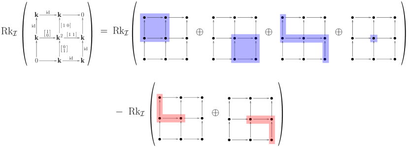
Figure 5. Minimal rank decomposition of the generalized rank invariant of the module $M$ from Figure 2 over the full collection $\mathcal{I}$ of intervals in the $3\times 3$ grid. Blue is for intervals in $\mathcal{R}$, while red is for intervals in $\mathcal{S}$.

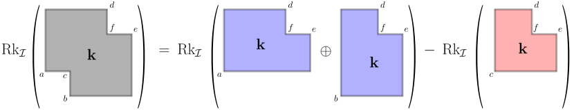
Figure 6. Taking $\mathcal{I}$ to be the collection of all intervals with one generator and at most two cogenerators (which includes in particular all rectangles), the generalized rank invariant of the interval 2-parameter persistence module $\mathbf{k}_{I}$ on the left-hand side decomposes minimally as the difference between the generalized rank invariants of the two modules on the right-hand side. Blue is for intervals in $\mathcal{R}$ while red is for intervals in $\mathcal{S}$.

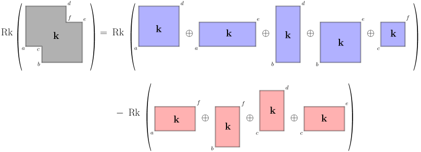
Figure 7. The usual rank invariant of the interval module $\mathbf{k}_{I}$ on the left-hand side decomposes minimally as the difference between the usual rank invariants of the two rectangle-decomposable modules on the right-hand side. Blue is for rectangles in $\mathcal{R}$ while red is for rectangles in $\mathcal{S}$.

Figures 5 and 6 illustrate Corollary 5.1, while Figures 3 and 7 illustrate Corollary 5.2.

To compute the minimal rank decompositions, we can apply the formula of Corollary 3.5, which reformulates as follows in the case of the usual rank invariant of a pfd persistence module $M$ indexed over a finite grid $G=\prod_{i=1}^{d}\llbracket 1,n_{i}\rrbracket\subset{\mathbb{R}}^{d}$:

(5.1) $$\forall s\leq t\in G,\ \alpha_{\langle s,t\rangle}=\sum_{\begin{smallmatrix}s^{\prime}\leq s\\ \|s^{\prime}-s\|_{\infty}\leq 1\end{smallmatrix}}\sum_{\begin{smallmatrix}t^{\prime}\geq t\\ \|t^{\prime}-t\|_{\infty}\leq 1\end{smallmatrix}}(-1)^{\|s^{\prime}-s\|_{1}+\|t^{\prime}-t\|_{1}}\,\operatorname{Rk}M(s^{\prime},t^{\prime}).$$

The case $d=1$ gives the well-known inclusion-exclusion formula relating the persistence diagram of a one-parameter persistence module to its rank invariant [13]. The case $d=2$ gives the inclusion-exclusion formula for computing the multiplicities of summands in rectangle-decomposable 2-parameter persistence modules [7].

Figure 7 illustrates (5.1) on an interval module $\mathbf{k}_{I}$ in a finite 2-d grid. Indeed, on such modules, (5.1) yields the following expression for the minimal rank decomposition of $\operatorname{Rk}\mathbf{k}_{I}$:

$$\mathcal{R} :=\left\{\langle g_{u},c_{v}\rangle\mid g_{u}\leq c_{v}\ \mbox{and}\ 2u\equiv 2v\!\!\!\!\mod 2\right\},$$

$$\mathcal{S} :=\left\{\langle g_{u},c_{v}\rangle\mid g_{u}\leq c_{v}\ \mbox{and}\ 2u\not\equiv 2v\!\!\!\!\mod 2\right\},$$

where $g_{1},\cdots,g_{k}$ are the generators of $\mathbf{k}_{I}$ (sorted by increasing abscissae), $c_{1},\cdots,c_{l}$ are its co-generators (sorted likewise), $g_{i+\frac{1}{2}}:=g_{i}\vee g_{i+1}$ (join) for each $i\in{\llbracket 1,k-1\rrbracket}$, and $c_{j+\frac{1}{2}}:=c_{j}\wedge c_{j+1}$ (meet) for each $j\in{\llbracket 1,l-1\rrbracket}$.

Remark 5.3.

In the general case where $G=\prod_{i=1}^{d}\llbracket 1,n_{i}\rrbracket\subset{\mathbb{R}}^{d}$, by applying (5.1) to every pair of comparable indices $s\leq t\in G$ in sequence, one computes the minimal rank decomposition of the usual rank invariant in time $O\left(2^{2d}\,\#\{{\leq}_{G}\}\right)$, assuming constant-time access to the ranks $\operatorname{Rk}M(s^{\prime},t^{\prime})$ and constant-time arithmetic operations. This bound is in $O\left(2^{2d}\,\prod_{i=1}^{d}n_{i}^{2}\right)$, and when $d$ is fixed, it is linear in the size of the encoding of the usual rank invariant as a map $\{{\leq}_{G}\}\to{\mathbb{Z}}$. When the module $M$ comes from a simplicial filtration over the grid $G$ with $n=\max_{i}n_{i}$ simplices in total, the usual rank invariant itself can be pre-computed and stored, e.g. by naively computing the ranks $\operatorname{Rk}M(s,t)$ for each pair $s\leq t\in G$ independently, which takes $O(n^{2d+\omega})$ time in total, where $2\leq\omega<2.373$ is the exponent for matrix multiplication [27]. Adding in the computation time for the minimal rank decomposition yields a bound in $O(n^{2d+\omega}+(2n)^{2d})$. While naive, this approach already compares favorably, in terms of running time, to the computation of other (stronger) invariants such as for instance the direct-sum decomposition of $M$—for which the best known algorithm runs in $O(n^{d(2\omega+1)})$ time [16]. Moreover, the running time of computing the minimal rank decomposition is dominated by the running time of pre-computing the usual rank invariant, for which there is room for improvement. In the special case where $d=2$ for instance, assuming the filtration is $1$-critical (i.e. each simplex has a unique minimal time of appearance in the filtration), there is an $O(n^{4})$-time algorithm to compute the usual rank invariant [7], and computing its minimal rank decomposition also takes $O(n^{4})$ time. By comparison, the best known algorithm to compute the direct-sum decomposition of $M$ in this setting takes $O(n^{2\omega+1})$ time [16], and computing the line arrangement data structure in RIVET takes $O(n^{5})$ time in the worst case [25].

5.2. The $\mathbb{R}^{d}$ case

Note first that ${\mathbb{R}}^{d}$ is an upper semi-lattice (in fact it is a complete lattice), so the results of Section 4.4 apply. The rectangles in this context are right-open rectangles, i.e. products of $d$ right-open intervals of the real line.

Theorem 5.4.

For the poset $\mathbb{R}^{d}$, the set

$$\{\mathbf{k}_{[a_{1},b_{1})\times\cdots\times[a_{d},b_{d})}]\mid a_{i}<b_{i}\in\mathbb{R}\cup\{\infty\}\}$$

is a basis of $\operatorname{K_{0}}(\mathcal{E}_{\operatorname{Rk}}^{\rm fp})$.

The proof uses the following intermediate result:

Lemma 5.5.

Assume ${I}=\bigcup_{i=1}^{n}{I}_{i}$, with each ${I}_{i}$ being a down-set in the poset ${I}$. Then, the sequence

$$0\to\mathbf{k}_{{I}}\to\bigoplus_{i=1}^{n}\mathbf{k}_{{I}_{i}}\to\bigoplus_{i<j}\mathbf{k}_{{I}_{i}\cap{I}_{j}}\to\bigoplus_{i<j<\ell}\mathbf{k}_{{I}_{i}\cap{I}_{j}\cap{I}_{\ell}}\to\cdots\to\mathbf{k}_{\bigcap_{i}I_{i}}\to 0$$

with component maps

$$\mathbf{k}_{\cap_{i\in X}{I}_{i}}\to\mathbf{k}_{\cap_{i\in Y}{I}_{i}}\colon\begin{cases}(-1)^{\#\{x\in X\mid x<y\}}\,\text{projection}&\text{if }Y=X\cup\{y\}\\ 0&\text{otherwise}\end{cases}$$

is rank exact. Note that the assumption that each ${I}_{i}$ is a down-set in ${I}$ guarantees the projections in the component maps to be well-defined.

Proof.

We employ induction on $n$. Let ${I}^{\prime}=\bigcup_{i=2}^{n}{I}_{i}$. The short exact sequence

$$0\to\mathbf{k}_{{I}}\to\mathbf{k}_{{I}_{1}}\oplus\mathbf{k}_{{I}^{\prime}}\to\mathbf{k}_{{I}_{1}\cap{I}^{\prime}}\to 0$$

is rank exact. Inductively, we have rank exact sequences for ${I}^{\prime}$ and for ${I}_{1}\cap{I}^{\prime}=\bigcup_{i=2}^{n}{I}_{1}\cap{I}_{i}$ as in the two rows of the following diagram.

We can add the vertical arrows and check that the entire diagram commutes (for appropriate sign conventions). In particular its total complex is rank exact again. Putting this total complex in the upper row, we obtain the following commutative diagram.

Choosing the vertical arrows to be inclusion of and projection to the corresponding summand we obtain a new commutative diagram. Again we form the total complex, and observe that up to homotopy the two copies of $\mathbf{k}_{{I}^{\prime}}$ and the two copies of $\mathbf{k}_{{I}_{1}\cap{I}^{\prime}}$ cancel. Thus we get the rank exact sequence in the statement of the lemma. ∎

Proof of Theorem 5.4.

Note that

$$\langle\mathbf{a},\mathbf{b}\langle=\bigcup_{i=1}^{d}[a_{1},\infty)\times\cdots\times[a_{i-1},\infty)\times[a_{i},b_{i})\times[a_{i+1},\infty)\times\cdots\times[a_{d},\infty),$$

and all the sets on the right-hand side are down-sets in $\langle\mathbf{a},\mathbf{b}\langle$. Thus, Lemma 5.5 applies. In particular, any $[\mathbf{k}_{\langle\mathbf{a},\mathbf{b}\langle}]$ is a linear combination of vectors in our candidate basis, which therefore generates $\operatorname{K_{0}}(\mathcal{E}_{\operatorname{Rk}}^{\rm fp})$.

The linear independence follows from Proposition 2.10—alternatively, linear independence can also be verified by carefully analyzing the base change from the basis of Theorem 4.16 to the candidate basis here. ∎

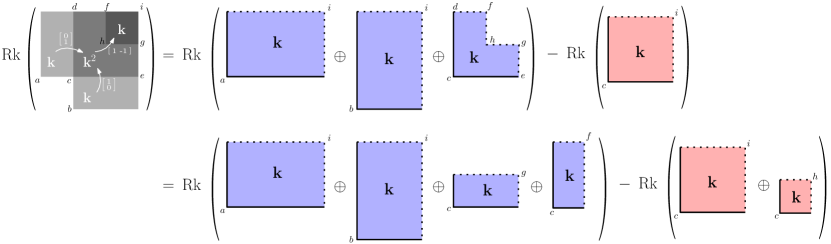
Figure 8. Left: an indecomposable persistence module with $2$ generators, one at $a$ and one at $b$, and a relation equating them at $h$ (indices $d,e,f,g,i$ lie at infinity). Right: minimal rank decompositions of the usual rank invariant of the module, respectively over the lower hooks (top row) and over the right-open rectangles (bottom row). Blue is for intervals in $\mathcal{R}$ while red is for intervals in $\mathcal{S}$. Solid boundaries belong to the intervals, while dotted boundaries do not.

Combining Theorems 4.16 and 5.4 yields the following result—see also Figure 8 for an illustration:

Corollary 5.6.

The usual rank invariant of every finitely presented persistence module $M$ over ${\mathbb{R}}^{d}$ admits a unique minimal rank decomposition over the lower hooks in ${\mathbb{R}}^{d}$. Likewise, $\operatorname{Rk}M$ admits a unique minimal rank decomposition over the right-open rectangles in ${\mathbb{R}}^{d}$.

5.3. Restrictions to lines

As ${\mathbb{R}}^{d}$ is a lattice, we can apply Proposition 2.16 to restrictions to sublattices, in particular to lines. A line $\ell$ in ${\mathbb{R}}^{d}$ is called strictly monotone if it can be parametrized by $\lambda\mapsto(1-\lambda)s+\lambda t$ where $s,t\in{\mathbb{R}}^{d}$ are fixed with coordinates $s_{i}<t_{i}$ for every $i=1,\cdots,d$.

Corollary 5.7.

Let $M$ be a pfd persistence module over ${\mathbb{R}}^{d}$ such that the usual rank invariant $\operatorname{Rk}M$ admits a rank decomposition $(\mathcal{R},\mathcal{S})$. Then, for any strictly monotone line $\ell$ in ${\mathbb{R}}^{d}$, $(\mathcal{R},\mathcal{S})$ restricts to a rank decomposition $({\mathcal{R}}_{|\ell},{\mathcal{S}}_{|\ell})$ of $\operatorname{Rk}{M}_{|\ell}$.

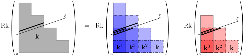
Figure 9. Restricting an interval module $\mathbf{k}_{I}$ to a strictly monotone line $\ell$ (left) yields a restriction of the minimal rank decomposition of $\operatorname{Rk}\mathbf{k}_{I}$ to $\ell$ (right)—for clarity, the rectangles’ boundaries are shown with different line styles. Here, the restricted rank decomposition is not minimal, as the two interval summands of $\mathbf{k}_{\mathcal{S}|_{\ell}}$ cancel out with two of the three interval summands of $\mathbf{k}_{\mathcal{R}|_{\ell}}$.

Note that the restriction of a minimal decomposition may not be minimal, as different rectangles in $\mathcal{R}$ and $\mathcal{S}$ may restrict to the same 1-d interval—see Figure 9 for an illustration. However, by Corollary 2.12, the minimal rank decomposition $(\mathcal{R}^{*},\mathcal{S}^{*})$ of $\operatorname{Rk}M_{|\ell}$ is easily obtained by removing all the common elements in ${\mathcal{R}}_{|\ell}$ and ${\mathcal{S}}_{|\ell}$. Furthermore, as illustrated in Figure 9 and formalized in the following result, $(\mathcal{R}^{*},\mathcal{S}^{*})$ actually coincides with the persistence barcode of the one-parameter module $M|_{\ell}$.

Corollary 5.8.

Every pfd persistence module $M$ indexed over the real line admits a unique minimal rank decomposition $(\mathcal{R},\mathcal{S})$, given by $\mathcal{R}=\textnormal{Dgm}\,M$, the persistence barcode of $M$, and $\mathcal{S}=\emptyset$.

Proof.

Follows from the structure theorem for pfd one-parameter persistence modules [15], combined with our Corollary 2.12. ∎

5.4. Stability

We conclude this section by saying a few words about the stability of our rank decompositions. Recall from Corollary 2.13 that we have $\mathbf{k}_{\mathcal{R}}\oplus\mathbf{k}_{\mathcal{S}^{\prime}}\simeq\mathbf{k}_{\mathcal{R}^{\prime}}\oplus\mathbf{k}_{\mathcal{S}}$ for any two rank decompositions $(\mathcal{R},\mathcal{S})$ and $(\mathcal{R}^{\prime},\mathcal{S}^{\prime})$ of the same persistence module $M$, or of two persistence modules $M,M^{\prime}$ sharing the same (usual) rank invariant. In effect, this is telling us that two rank decompositions are equivalent whenever their ground modules have the same rank invariant. Using the matching (pseudo-)distance $\mathrm{d}_{\mathrm{match}}$ from [22], we can derive a metric version of this statement (Theorem 5.9), which bounds the defect of equivalence between two rank decompositions in terms of the fibered distance between the rank invariants of their ground modules. Recall that the matching distance between two pfd persistence modules $M,N$ in ${\mathbb{R}}^{d}$ is defined as follows:

(5.2) $$\mathrm{d}_{\mathrm{match}}(M,N)=\sup_{\ell\ \text{strictly monotone}}\ \omega(\ell)\ \mathrm{d}_{\mathrm{b}}(M|_{\ell},N|_{\ell}),$$

where $\mathrm{d}_{\mathrm{b}}$ denotes the usual bottleneck distance between one-parameter persistence modules, and where the weight $\omega(\ell)$ assigned to any strictly monotone line $\ell$ parametrized by $\lambda\mapsto(1-\lambda)s+\lambda t$ with $\lambda$ ranging over ${\mathbb{R}}$ while $s,t$ are fixed in ${\mathbb{R}}^{d}$ and satisfy $s_{i}<t_{i}$ for each $i=1,\cdots,d$, is

$$\omega(\ell)=\frac{\min_{i}t_{i}-s_{i}}{\max_{i}t_{i}-s_{i}}>0.$$

Theorem 5.9.

Let $M,M^{\prime}$ be pfd persistence modules indexed over ${\mathbb{R}}^{d}$. Then, for any rank decompositions $(\mathcal{R},\mathcal{S})$ and $(\mathcal{R}^{\prime},\mathcal{S}^{\prime})$ of $M$ and $M^{\prime}$ respectively, we have:

$$\mathrm{d}_{\mathrm{match}}(\mathbf{k}_{\mathcal{R}}\oplus\mathbf{k}_{\mathcal{S}^{\prime}},\mathbf{k}_{\mathcal{R}^{\prime}}\oplus\mathbf{k}_{\mathcal{S}})\leq\mathrm{d}_{\mathrm{match}}(M,M^{\prime}).$$

Proof.

Take any strictly monotone line $\ell$ in ${\mathbb{R}}^{d}$. By (5.2), we have:

$$\mathrm{d}_{\mathrm{b}}(M_{|\ell},M^{\prime}_{|\ell})\leq\omega(\ell)^{-1}\,\mathrm{d}_{\mathrm{match}}(M,M^{\prime}).$$

Meanwhile, by Corollary 5.7, $(\mathcal{R}_{|\ell},\mathcal{S}_{|\ell})$ is a rank decomposition of $M_{|\ell}$, and $(\mathcal{R}^{\prime}_{|\ell},\mathcal{S}^{\prime}_{|\ell})$ is a rank decomposition of $M^{\prime}_{|\ell}$. By Proposition 2.10, we then have $M_{|\ell}\oplus\mathbf{k}_{\mathcal{S}_{|\ell}}\simeq\mathbf{k}_{\mathcal{R}_{|\ell}}$ and $M^{\prime}_{|\ell}\oplus\mathbf{k}_{\mathcal{S}^{\prime}_{|\ell}}\simeq\mathbf{k}_{\mathcal{R}^{\prime}_{|\ell}}$, from which we deduce:

$$\mathrm{d}_{\mathrm{b}}(M_{|\ell},M^{\prime}_{|\ell})\geq\mathrm{d}_{\mathrm{b}}(M_{|\ell}\oplus\mathbf{k}_{\mathcal{S}_{|\ell}}\oplus\mathbf{k}_{\mathcal{S}^{\prime}_{|\ell}},M^{\prime}_{|\ell}\oplus\mathbf{k}_{\mathcal{S}_{|\ell}}\oplus\mathbf{k}_{\mathcal{S}^{\prime}_{|\ell}})=\mathrm{d}_{\mathrm{b}}(\mathbf{k}_{\mathcal{R}_{|\ell}}\oplus\mathbf{k}_{\mathcal{S}^{\prime}_{|\ell}},\mathbf{k}_{\mathcal{R}^{\prime}_{|\ell}}\oplus\mathbf{k}_{\mathcal{S}_{|\ell}}).$$

Combined with the previous equation, this gives:

$$\mathrm{d}_{\mathrm{b}}(\mathbf{k}_{\mathcal{R}_{|\ell}}\oplus\mathbf{k}_{\mathcal{S}^{\prime}_{|\ell}},\mathbf{k}_{\mathcal{R}^{\prime}_{|\ell}}\oplus\mathbf{k}_{\mathcal{S}_{|\ell}})\leq\omega(\ell)^{-1}\,\mathrm{d}_{\mathrm{match}}(M,M^{\prime}).$$

The result follows then by taking the supremum on the left-hand side over all possible choices of strictly monotone lines $\ell$. ∎

It is worth pointing out that different choices of rank decompositions $(\mathcal{R},\mathcal{S})$ and $(\mathcal{R}^{\prime},\mathcal{S}^{\prime})$ for $M$ and $M^{\prime}$ may yield different values for the matching distance $\mathrm{d}_{\mathrm{match}}(\mathbf{k}_{\mathcal{R}}\oplus\mathbf{k}_{\mathcal{S}^{\prime}},\mathbf{k}_{\mathcal{R}^{\prime}}\oplus\mathbf{k}_{\mathcal{S}})$. It turns out that the rank decompositions that maximize this distance are precisely the minimal rank decompositions, which therefore satisfy a universal property also in terms of the metric between decompositions:

Proposition 5.10.

Let $M,M^{\prime}$ be pfd persistence modules indexed over ${\mathbb{R}}^{d}$. Then, for any rank decompositions $(\mathcal{R},\mathcal{S})$ and $(\mathcal{R}^{\prime},\mathcal{S}^{\prime})$ of $M$ and $M^{\prime}$ respectively, we have:

$$\mathrm{d}_{\mathrm{match}}(\mathbf{k}_{\mathcal{R}}\oplus\mathbf{k}_{\mathcal{S}^{\prime}},\mathbf{k}_{\mathcal{R}^{\prime}}\oplus\mathbf{k}_{\mathcal{S}})\leq\mathrm{d}_{\mathrm{match}}(\mathbf{k}_{\mathcal{R}^{*}}\oplus\mathbf{k}_{\mathcal{S}^{\prime*}},\mathbf{k}_{\mathcal{R}^{\prime*}}\oplus\mathbf{k}_{\mathcal{S}^{*}}),$$

where $(\mathcal{R}^{*},\mathcal{S}^{*})$ and $(\mathcal{R}^{\prime*},\mathcal{S}^{\prime*})$ are the minimal rank decompositions of $M$ and $M^{\prime}$ respectively—which exist as soon as $(\mathcal{R},\mathcal{S})$ and $(\mathcal{R}^{\prime},\mathcal{S}^{\prime})$ do, by Corollary 2.12.

Proof.

Let $\mathcal{T}:=\mathcal{R}\setminus\mathcal{R}^{*}=\mathcal{S}\setminus\mathcal{S}^{*}$, and $\mathcal{T}^{\prime}:=\mathcal{R}^{\prime}\setminus\mathcal{R}^{\prime*}=\mathcal{S}^{\prime}\setminus\mathcal{S}^{\prime*}$. Note that $\mathcal{T},\mathcal{T}^{\prime}$ are well-defined by Theorem 2.11. Then, for any strictly monotone line $\ell$, we have:

$$\mathrm{d}_{\mathrm{b}}(\mathbf{k}_{\mathcal{R}_{|\ell}}\oplus\mathbf{k}_{\mathcal{S}^{\prime}_{|\ell}},\mathbf{k}_{\mathcal{R}^{\prime}_{|\ell}}\oplus\mathbf{k}_{\mathcal{S}_{|\ell}}) =\mathrm{d}_{\mathrm{b}}(\mathbf{k}_{{\mathcal{R}^{*}}_{|\ell}}\oplus\mathbf{k}_{{\mathcal{S}^{\prime*}}_{|\ell}}\oplus\mathbf{k}_{\mathcal{T}_{|\ell}}\oplus\mathbf{k}_{\mathcal{T}^{\prime}_{|\ell}},\mathbf{k}_{{\mathcal{R}^{\prime*}}_{|\ell}}\oplus\mathbf{k}_{{\mathcal{S}^{*}}_{|\ell}}\oplus\mathbf{k}_{\mathcal{T}_{|\ell}}\oplus\mathbf{k}_{\mathcal{T}^{\prime}_{|\ell}})$$

$$\leq\mathrm{d}_{\mathrm{b}}(\mathbf{k}_{{\mathcal{R}^{*}}_{|\ell}}\oplus\mathbf{k}_{{\mathcal{S}^{\prime*}}_{|\ell}},\mathbf{k}_{{\mathcal{R}^{\prime*}}_{|\ell}}\oplus\mathbf{k}_{{\mathcal{S}^{*}}_{|\ell}}).$$

The result follows then after multiplying by $\omega(\ell)$ and taking the supremum on both sides over all possible choices of strictly monotone lines $\ell$. ∎

Finally, we can also bound the defect of equivalence between two rank decompositions in terms of the defect of isomorphism between their ground modules—measured by the interleaving distance $\mathrm{d}_{\mathrm{i}}$. This is a straight consequence of our Theorem 5.9 and of Theorem 1 from [22]:

Corollary 5.11.

Let $M,M^{\prime}$ be pfd persistence modules indexed over ${\mathbb{R}}^{d}$. Then, for any rank decompositions $(\mathcal{R},\mathcal{S})$ and $(\mathcal{R}^{\prime},\mathcal{S}^{\prime})$ of $M$ and $M^{\prime}$ respectively, we have:

$$\mathrm{d}_{\mathrm{match}}(\mathbf{k}_{\mathcal{R}}\oplus\mathbf{k}_{\mathcal{S}^{\prime}},\mathbf{k}_{\mathcal{R}^{\prime}}\oplus\mathbf{k}_{\mathcal{S}})\leq\mathrm{d}_{\mathrm{i}}(M,M^{\prime}).$$

6. Signed barcodes and prominence diagrams for multi-parameter persistence modules

In the context of topological data analysis, the minimal rank decomposition $(\mathcal{R},\mathcal{S})$ encodes visually the structure of the rank invariant of a persistence module $M\colon{\mathbb{R}}^{d}\to\mathrm{Vec}_{\mathbf{k}}$. In the particular case of the usual rank invariant, we saw in the examples of Section 5 that we get direct access to the following pieces of information:

• the rank $\operatorname{Rk}M(s,t)$ between any pair of indices $s\leq t\in{\mathbb{R}}^{d}$, obtained as the number of rectangles in $\mathcal{R}$ that contain both $s$ and $t$ minus the number of rectangles in $\mathcal{S}$ that contain both $s$ and $t$;

• the barcode of the restriction of $M$ to any strictly monotone line $\ell$, obtained by simplifying the restriction of $(\mathcal{R},\mathcal{S})$ to $\ell$, each bar of which comes from the intersection of a rectangle in $\mathcal{R}$ or $\mathcal{S}$ with $\ell$.

The main drawback of representing rectangles as rectangles is that their overlaid arrangement quickly becomes hard to read—see e.g. Figure 9.

6.1. Signed barcodes

An alternate representation of the rectangles is by their diagonal with positive slope in ${\mathbb{R}}^{d}$. We call this representation the signed barcode of $\operatorname{Rk}M$, where each bar is the diagonal (with positive slope) of a particular rectangle in $\mathcal{R}$ or $\mathcal{S}$, and where the sign is positive for bars coming from $\mathcal{R}$ and negative for bars coming from $\mathcal{S}$—see Figure 10 for an illustration. Like the rectangles, the bars are considered with multiplicity.

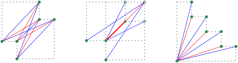
Figure 10. From left to right: signed barcodes corresponding to the usual rank decompositions of Figures 7, 8 (bottom row), and 9 respectively. Blue bars are diagonals of rectangles in $\mathcal{R}$ and therefore counted positively, while red bars are diagonals of rectangles in $\mathcal{S}$ and therefore counted negatively. The bars’ endpoints are marked in green (as a solid dot when the endpoint lies in the rectangle, as a circled dot when it does not—e.g. when it lies at infinity), to discriminate them from intersections. The thick red line segment in the center picture shows the overlap between a shorter red bar and a longer red bar sharing the same lower endpoint and slope.

The signed barcode of $\operatorname{Rk}M$ gives direct access to the same pieces of information as the rectangular representation—see Figure 11:

• the rank $\operatorname{Rk}M(s,t)$ between any pair of indices $s\leq t\in{\mathbb{R}}^{d}$ is obtained as the number of positive bars that connect the down-set $s^{-}=\{u\in{\mathbb{R}}^{d}\mid u\leq s\}$ to the up-set $t^{+}=\{u\in{\mathbb{R}}^{d}\mid u\geq t\}$, minus the number of negative bars that connect $s^{-}$ to $t^{+}$—exactly as with persistence barcodes in the one-parameter case (see Figure 1), except bars are now signed;

• the barcode of the restriction of $M$ to any strictly monotone line $\ell$ is obtained by simplifying the restriction of $(\mathcal{R},\mathcal{S})$ to $\ell$, each bar of which comes from the projection of a bar $(s,t)$ in the signed barcode onto $\ell$ according to the following rule—coming from the intersection of $\ell$ with the rectangle $\langle s,t\rangle$: project $s$ onto the point $s^{\prime}=\ell\cap\partial s^{+}$, and $t$ onto $t^{\prime}=\ell\cap\partial t^{-}$, if these two points exist and satisfy $s^{\prime}\leq t^{\prime}$ (otherwise the projection is empty).

Beyond these features, the signed barcode makes it possible to visually grasp the global structure of the usual rank invariant $\operatorname{Rk}M$, and in particular, to infer the directions along which topological features have the best chances to persist.

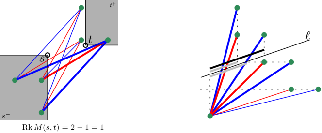
Figure 11. Left: computing $\operatorname{Rk}M(s,t)$ for a pair of indices $s\leq t$ (the thick bars are the ones connecting the down-set $s^{-}$ to the up-set $t^{+}$). Right: restricting the minimal rank decomposition of $\operatorname{Rk}M$ to a strictly monotone line $\ell$—the thick blue and red bars are the ones projecting to non-empty bars along $\ell$, and among those projections, the thick gray bars get cancelled out during the simplification while the thick black bar remains in the barcode of $M|_{\ell}$.

6.2. Extension to generalized rank invariants.

When the collection $\mathcal{I}$ of intervals under consideration contains more than just the rectangles, the intervals involved in the corresponding minimal rank decomposition $(\mathcal{R},\mathcal{S})$ of $M$ are no longer described by a single diagonal. Nevertheless, each interval ${I}\in\mathcal{R}\sqcup\mathcal{S}$ is still uniquely described by the collection of maximal rectangles included in it, or equivalently, by the collection $D_{I}$ of their diagonals with positive slope. We can then form a signed barcode for $(\mathcal{R},\mathcal{S})$ by putting together the bars coming from all the sets $D_{I}$, with positive signs when ${I}\in\mathcal{R}$ and with negative signs when ${I}\in\mathcal{S}$. The outcome is a decorated signed barcode, where the decoration groups the bars according to which element ${I}\in\mathcal{R}\sqcup\mathcal{S}$ they originate from—see Figure 12 (left) for an illustration. Notice that some bars coming from different collections $D_{I},D_{J}$ with opposite signs might cancel with each other in the process—for instance, in the example of Figure 12 (left), this would happen with bar $[c,d]$ if an extra rectangle summand $\mathbf{k}_{\langle c,d\rangle}$ was added to the interval module on the left-hand side of Figure 6. In practice, depending on the application, one may want to keep track of these cancellations in order to avoid losing information about the original rank decomposition $(\mathcal{R},\mathcal{S})$ in the final decorated signed barcode.

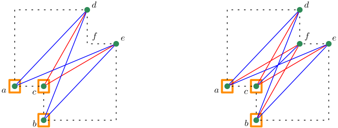
Figure 12. Decorated signed barcodes corresponding to the generalized rank decomposition of Figure 6. Left: keeping only the maximal rectangles included in each element ${I}\in\mathcal{R}\sqcup\mathcal{S}$. Right: keeping the entire minimal usual rank decomposition of each element ${I}\in\mathcal{R}\sqcup\mathcal{S}$—notice that the underlying undecorated signed barcode is identical to the one from Figure 10 (left). The orange squares indicate how the bars are grouped together according to their originating element ${I}\in\mathcal{R}\sqcup\mathcal{S}$.

A variant of the previous construction collects not only the maximal rectangles included in each element ${I}\in\mathcal{R}\sqcup\mathcal{S}$, but the whole minimal usual rank decomposition of $\mathbf{k}_{I}$, or equivalently, its corresponding usual signed barcode. As illustrated in Figure 12 (right), the outcome is a decorated version of the usual signed barcode of $M$, where the decoration indicates which element ${I}\in\mathcal{R}\sqcup\mathcal{S}$ each bar comes from. Indeed, it is easily seen that, once put together, the minimal usual rank decompositions of the $\mathbf{k}_{I}$ for ${I}$ ranging over $\mathcal{R}\sqcup\mathcal{S}$ form a usual rank decomposition of $M$. Notice that this decomposition may not be minimal, so, again, some bars coming from different elements $\mathbf{k}_{I},\mathbf{k}_{J}$ may cancel with each other in the resulting usual signed barcode of $M$. Whether to keep track of these cancellations (and thus to avoid losing information about the original rank decomposition) will depend on the application considered in practice, but in any case, the added value of computing rank decompositions over larger collections of intervals than just the rectangles is to provide decorations (possibly involving extra cancelling bars) to the usual signed barcode of $M$, allowing for a higher-level interpretation by the user. We shall keep this in mind when interpreting our experimental results in Section 7.

6.3. Signed prominence diagrams

To each bar with endpoints $s\leq t$ in the usual signed barcode of a module $M:{\mathbb{R}}^{d}\to\mathrm{Vec}_{\mathbf{k}}$, we can associate its signed prominence, which is the $d$-dimensional vector $t-s$ if the bar corresponds to a rectangle in $\mathcal{R}$, or $s-t$ if the bar corresponds to a rectangle in $\mathcal{S}$. We call signed prominence diagram of $M$ the resulting collection of vectors in ${\mathbb{R}}^{d}$—see Figure 13 for an illustration.

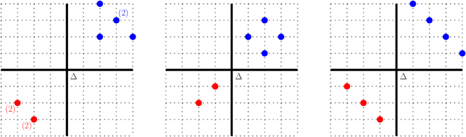
Figure 13. The signed prominence diagrams corresponding to the signed barcodes of Figure 10, in the same order. Blue dots correspond to blue bars (hence to rectangles in $\mathcal{R}$), while red dots correspond to red bars (hence to rectangles in $\mathcal{S}$). Multiplicities differring from $1$ are indicated explicitly. The union $\Delta$ of the two coordinate axes plays the role of the diagonal, as explained below.

Example 6.1.

In the one-parameter setting, the signed prominence diagram encodes the lengths of the bars in the unsigned barcode, i.e. the vertical distances of the points to the diagonal in the persistence diagram. It is a discrete measure on the real line.

In a signed prominence diagram, the union $\Delta$ of the hyperplanes perpendicular to the coordinate axes and passing through the origin plays the role of the diagonal: a bar whose signed prominence lies close to $\Delta$ can be viewed as noise, whereas a bar whose signed prominence lies far away from $\Delta$ can be considered significant for the structure of the module $M$. The right way to formalize this intuition is via smoothings, as in the one-parameter case.

Definition 6.2.

Given a persistence module $M$ indexed over ${\mathbb{R}}^{d}$, and a vector $\varepsilon\in{\mathbb{R}}_{\geq 0}^{d}$, the $\varepsilon$-shift $M[\varepsilon]$ is the module defined pointwise by $M[\varepsilon](t)=M(t+\varepsilon)$ and $M[\varepsilon](s\leq t)=M(s+\varepsilon\leq t+\varepsilon)$. There is a canonical morphism of persistence modules $M\to M[\varepsilon]$, whose image is called the $\varepsilon$-smoothing of $M$, denoted by $M^{\varepsilon}$.

Example 6.3.

The $\varepsilon$-shift of a rectangle module $\mathbf{k}_{{R}}$ is the rectangle module $\mathbf{k}_{{R}-\varepsilon}$, where by definition ${R}-\varepsilon=\{t-\varepsilon\mid t\in{R}\}$. The $\varepsilon$-smoothing of $\mathbf{k}_{{R}}$ is the rectangle module $\mathbf{k}_{{R}^{\varepsilon}}$, where by definition ${R}^{\varepsilon}$ is the rectangle ${R}\cap({R}-\varepsilon)$, obtained from ${R}$ by shifting the upper-right corner $\max{R}$ by -$\varepsilon$. Note that $\mathbf{k}_{{R}^{\varepsilon}}$ is the trivial module whenever ${R}\cap({R}-\varepsilon)=\emptyset$, i.e. whenever the shifted upper-right corner is no longer greater than or equal to the lower-left corner.

As it turns out, usual rank decompositions commute with smoothings, more precisely:

Lemma 6.4.

Suppose $M:{\mathbb{R}}^{d}\to\mathrm{Vec}_{\mathbf{k}}$ admits a usual rank decomposition $(\mathcal{R},\mathcal{S})$. Then, for any $\varepsilon\in{\mathbb{R}}_{\geq 0}^{d}$, the pair $(\mathcal{R}^{\varepsilon},\mathcal{S}^{\varepsilon})$ where $\mathcal{R}^{\varepsilon}=\{{R}^{\varepsilon}\mid{R}\in\mathcal{R}\}$ and $\mathcal{S}^{\varepsilon}=\{{S}^{\varepsilon}\mid{S}\in\mathcal{S}\}$ is a usual rank decomposition of $M^{\varepsilon}$. When $(\mathcal{R},\mathcal{S})$ is minimal, so is $(\mathcal{R}^{\varepsilon},\mathcal{S}^{\varepsilon})$ after removing the empty rectangles from $\mathcal{R}^{\varepsilon}$ and $\mathcal{S}^{\varepsilon}$.

Proof.

For any indices $s\leq t\in{\mathbb{R}}^{d}$, the commutativity of the square

implies that $\operatorname{Rk}M^{\varepsilon}(s,t)=\operatorname{Rk}M(s,t+\varepsilon)$. Then, the usual rank decomposition of $M$ at indices $(s,t+\varepsilon)$ gives:

$$\operatorname{Rk}M^{\varepsilon}(s,t)=\operatorname{Rk}M(s,t+\varepsilon) =\sum_{{R}\in\mathcal{R}}\operatorname{Rk}\mathbf{k}_{R}(s,t+\varepsilon)-\sum_{{S}\in\mathcal{S}}\operatorname{Rk}\mathbf{k}_{S}(s,t+\varepsilon)$$

$$=\sum_{{R}\in\mathcal{R}}\operatorname{Rk}\mathbf{k}_{R}^{\varepsilon}(s,t)-\sum_{{S}\in\mathcal{S}}\operatorname{Rk}\mathbf{k}_{S}^{\varepsilon}(s,t)$$

(Example 6.3) $$=\sum_{{R}\in\mathcal{R}}\operatorname{Rk}\mathbf{k}_{{R}^{\varepsilon}}(s,t)-\sum_{{S}\in\mathcal{S}}\operatorname{Rk}\mathbf{k}_{{S}^{\varepsilon}}(s,t).$$

When $(\mathcal{R},\mathcal{S})$ is minimal, the minimality of $(\mathcal{R}^{\varepsilon},\mathcal{S}^{\varepsilon})$ after removing the empty rectangles comes from the fact that each ${R}^{\varepsilon}$ is obtained from ${R}$ by shifting its upper-right corner $\max{R}$ by -$\varepsilon$, so ${R}^{\varepsilon}={S}^{\varepsilon}\neq\emptyset$ implies ${R}={S}$. ∎

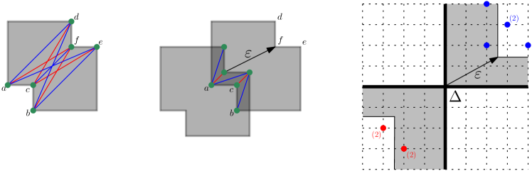
Figure 14. Behavior of the signed barcode and prominence diagram under $\varepsilon$-smoothing. Left: the input module $M$ from Figure 7, overlaid with its signed barcode. Center: the $\varepsilon$-smoothing $M^{\varepsilon}$ of $M$, shown in dark gray and overlaid with its own signed barcode—obtained by shifting the right endpoints in the signed barcode of $M$ by -$\varepsilon$. Right: effect of the  $\varepsilon$-smoothing on the signed prominence diagram.

Thus, the effect of $\varepsilon$-smoothing $M$ on its signed barcode is to shift the right endpoints of the bars by -$\varepsilon$, removing those bars for which the shifted right endpoint is no longer greater than or equal to the left endpoint. The effect on its signed prominence diagram is to shift the positive vectors by -$\varepsilon$ and the negative vectors by $\varepsilon$, removing those vectors that cross $\Delta$. Alternatively, one can inflate $\Delta$ by $\varepsilon$, and remove the vectors that lie in the inflated $\Delta$, as illustrated in Figure 14.

So, the remoteness of the signed prominence of a bar from $\Delta$, or equivalently, the width of the rectangle corresponding to this bar in the usual rank decomposition of $M$, measures how resilient that bar or rectangle is under smoothings of $M$, and thus how important it is for the structure of the usual rank invariant.

7. Experiments

In this section we consider the signed barcodes in three different two-parameter settings. In the first experiment (Section 7.2), our point set has three distinct holes, and we will see how these holes can be inferred from the signed barcode. In the second experiment (Section 7.3), we explore the stability properties of the signed barcodes by considering a family of point sets sampled from the unit circle with an increasing amount of noise. In the final experiment (Section 7.4), we apply our methods in the context of two-parameter clustering. Before getting to the details of the experiments, we recall some helpful basic concepts from topological data analysis in Section 7.1.

Remark 7.1.

Since we are working with two-parameter persistence modules throughout, in practice we have chosen to rely entirely on RIVET [25] to compute the usual rank invariant, mainly for the sake of simplicity and speed of implementation. As pointed out in Remark 5.3 and further discussed in Section 8, the use of RIVET—or part thereof—is not mandatory but can be considered as an option.

7.1. General constructions

Let $(P,d)$ denote a finite metric space. The neighborhood graph at scale $r$ is the graph $N(P)_{r}$ with vertex set $P$, and with an edge connecting $p$ and $q$ if $d(p,q)\leq r$. The Vietoris–Rips complex at scale $r$, ${\rm VR}(P)_{r}$, is defined as the clique complex on $N(P)_{r}$, i.e. the largest simplicial complex having $N(P)_{r}$ as its 1-skeleton. The Vietoris–Rips complex is an important tool in single-parameter persistent homology and it can be further refined in the presence of a real valued function $f\colon P\to{\mathbb{R}}$: the Vietoris–Rips bifiltration of ${\rm VR}(P)_{\infty}$ (with respect to $f$) is given by

$${\rm VR}(P,f)_{r,s}:={\rm VR}(f^{-1}(-\infty,s])_{r}.$$

Applying simplicial homology with coefficients in a field $\mathbf{k}$ yields a persistence module $M$ over ${\mathbb{R}}^{2}$,

$$M(r,s)=H_{p}({\rm VR}(P,f)_{r,s}).$$

When considering points in the plane it is convenient to visualize the Vietoris–Rips bifiltration by the bifiltration of the plane given by $f$ and the distance function, i.e.

$$U^{f}_{r,s}=\left\{z\in{\mathbb{R}}^{2}:\min_{p\in P,f(p)\leq s}||p-z||\leq r/2.\right\}$$

As is well-known, $H_{p}(U^{f})$ offers only an approximation of $H_{p}({\rm VR}(P,f))$, and thus there might be slight homological discrepancies between the planar subsets as visualized, and the Vietoris–Rips bifiltration.

In practice we will consider a discretization of $M$. This is done by first selecting a finite number of thresholds $X=\{r_{0},\ldots,r_{g_{1}-1}\}$ and $Y=\{s_{0}\ldots,s_{g_{2}-1}\}$ for $r$ and $s$, respectively, and then restricting $M$ to the grid $X\times Y$. In all the plots we will identify $X\times Y$ with the grid $\{0,1,\ldots,g_{1}-1\}\times\{0,1,\ldots,g_{2}-1\}$. By Proposition 2.16 we know that if $(\mathcal{R},\mathcal{S})$ is a rank decomposition of $M$, then $(\mathcal{R}|_{X\times Y},\mathcal{S}|_{X\times Y})$ is a rank decomposition of $M|_{X\times Y}$.

7.2. Experiment 1: planar points and the height function

• The point set $P$ consists of 150 planar points as shown in Figure 15 (left).

• The function $f$ is the height function, i.e. $f(p_{x},p_{y})=p_{y}$.

• The homology degree is 1 and $\mathbf{k}={\mathbb{Z}}_{2}$.

• The discretizations are given by restriction to the grids $G_{1}=\{r_{0},\ldots,r_{49}\}\times\{s_{0},\ldots,s_{49}\}$ and $G_{2}=\{r_{4},r_{9},\ldots,r_{49}\}\times\{s_{4},s_{9},\ldots,s_{49}\}$. The values $r_{i}$ are chosen such that the difference $r_{i+1}-r_{i}$ is constant, while the values $s_{i}$ are selected such that each interval $[s_{i},s_{i+1})$ contains the same number of function values.

The point set exhibits three significant holes of varying sizes appearing at different heights. Moving from bottom and up we denote these holes by A, B and C, respectively. The evolution of these holes in the bifiltration is shown in Figure 15 (right), and the associated signed barcodes of $M|_{G_{1}}$ and $M|_{G_{2}}$ are shown in Figure 16.

Let us first consider the coarser grid, whose signed barcode is shown in Figure 16(b). To the left in the figure there are a several features (indicated by a line of increased thickness) persisting only in the vertical direction. These features correspond to tiny loops formed by “noise” in the sampling, as can be seen in the first column of Figure 15 (right). The holes A and C are generated at a unique index and therefore each of them gives rise to a single bar in the signed barcode. On the other hand, hole B appears at two incomparable indices and therefore gives rise to two rectangles in $\mathcal{R}|_{G_{2}}$ born at incomparable grades, and a rectangle in $\mathcal{S}|_{G_{2}}$ accounting for double counting. Although one in general cannot infer a decorated rank decomposition from the ordinary rank invariant, the pattern of the bars suggests a generalized rank decomposition as shown in Figure 17(b). We see that these intervals correspond precisely to the supports shown in Figure 15. The existence of a “single” feature could be confirmed by computing generalized rank invariants.

Shifting our focus to the finer grid, the first thing we observe is that the choice of a finer discretization increases the number of bars in the signed barcode. This is not surprising as the same feature will now appear at an additional number of incomparable points. Again, the collection of bars strongly suggests the features persisting over certain intervals as seen in Figure 17(a).

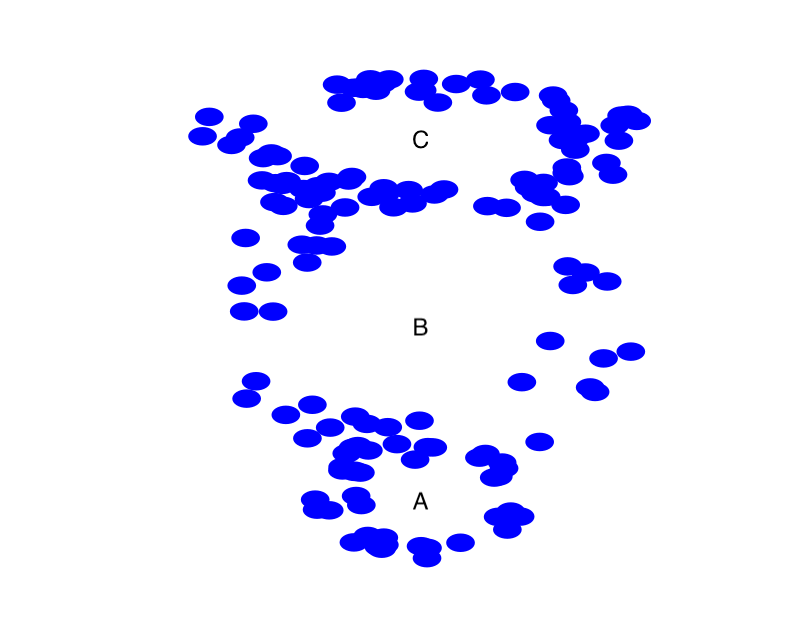
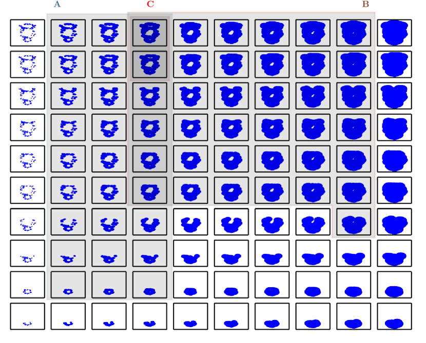
Figure 15. Left: The point set in Experiment 1. Right: The associated bifiltration of the distance and height functions. The lifespan of each 1-dimensional feature A, B, C in the bifiltration is highlighted in a specific color.

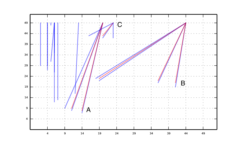
(a)

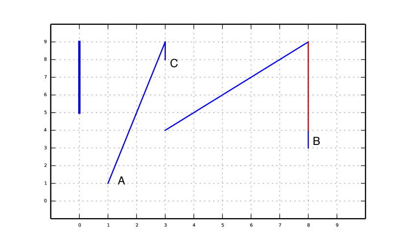
(b)

Figure 16. The signed barcode of Experiment 1 for two different choices of grid-size: $50\times 50$ (A) and $10\times 10$ (B).

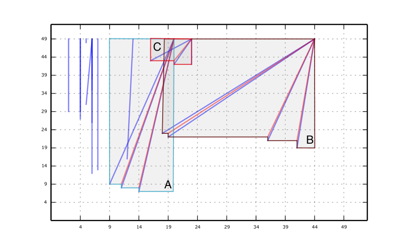
(a)

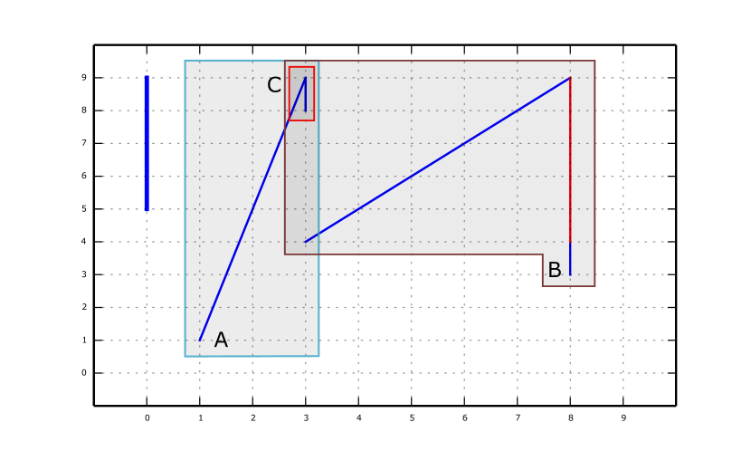
(b)

Figure 17. The supports of the three features A, B and C in Experiment 1 for our two choices of grid-size: $50\times 50$ (left) and $10\times 10$ (right). The supports in the $10\times 10$ grid coincide with the supports shown in Figure 15. They have been slightly inflated here for better readability.

7.3. Experiment 2: noisy circles and stability

• Six point sets $P_{0},\ldots,P_{5}$, where $P_{0}$ consists of 80 points that are evenly placed along the unit circle, and $P_{i}=\{p+i\,\varepsilon_{p}:p\in P\}$ where $\varepsilon_{p}$ is a fixed random vector with coordinates sampled independently and uniformly from $(-0.1,0.1)$. See Figure 18.

• The function $f$ is the height function, i.e. $f(p_{x},p_{y})=p_{y}$.

• The homology degree is 1 and $\mathbf{k}={\mathbb{Z}}_{2}$.

• The discretization is obtained by restriction to $G_{1}=\{r_{0},\ldots,r_{39}\}\times\{s_{0},\ldots,s_{39}\}$, where the values are chosen such that the differences $r_{i+1}-r_{i}$ and $s_{j+1}-s_{j}$ are constant. For the purpose of visualization we shall use the coarser grid $G_{2}=\{r_{3},r_{7},\ldots,r_{39}\}\times\{s_{3},s_{7},\ldots,s_{39}\}$ — see Figure 19.

The purpose of this experiment is evidently to observe the evolution of the signed barcodes as the points are moving linearly from $\{p\}$ to $\{p+5\,\varepsilon_{p}\}$. The signed barcodes are shown in (A) through (F) of Figure 20. We observe the following:

• ($P_{0}$) As expected: at lower heights, the feature appears at larger distance thresholds than at higher heights.

• ($P_{1}$) With the introduction of noise in the data, the feature persists longer at lower heights, and this causes the addition of two near-horizontal generators around height index 30, as well as a vertical generator around scale index 33. To account for double-counting of the rank, two near-horizontal co-generators and one vertical co-generator appear as well. Note that while the second to last column of Figure 19 suggests the presence of a non-trivial $H_{1}$, that is not the case when working with the Vietoris–Rips complex.

• ($P_{2}-P_{5}$) As the perturbation increases the support of the signed barcode corresponding to the circular signal in the data gradually shrinks: it appears at a later scale and persists for a shorter amount of time. Furthermore, the noise has introduces several short-lived cycles in the data, giving rise to an increasing amount of near-vertical lines to the left in the plot.

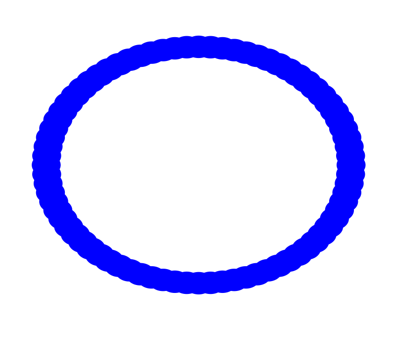
(a) $P_{0}$

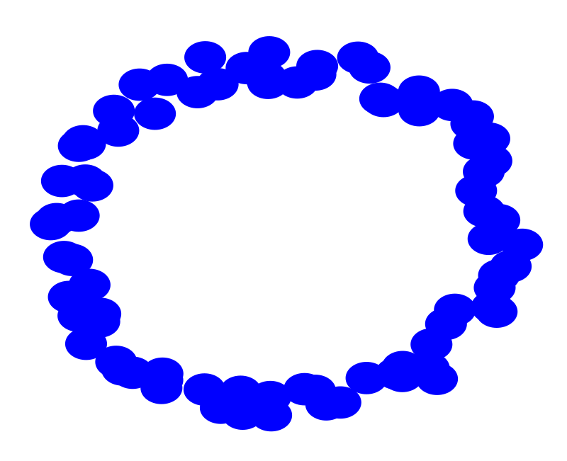
(b) $P_{1}$

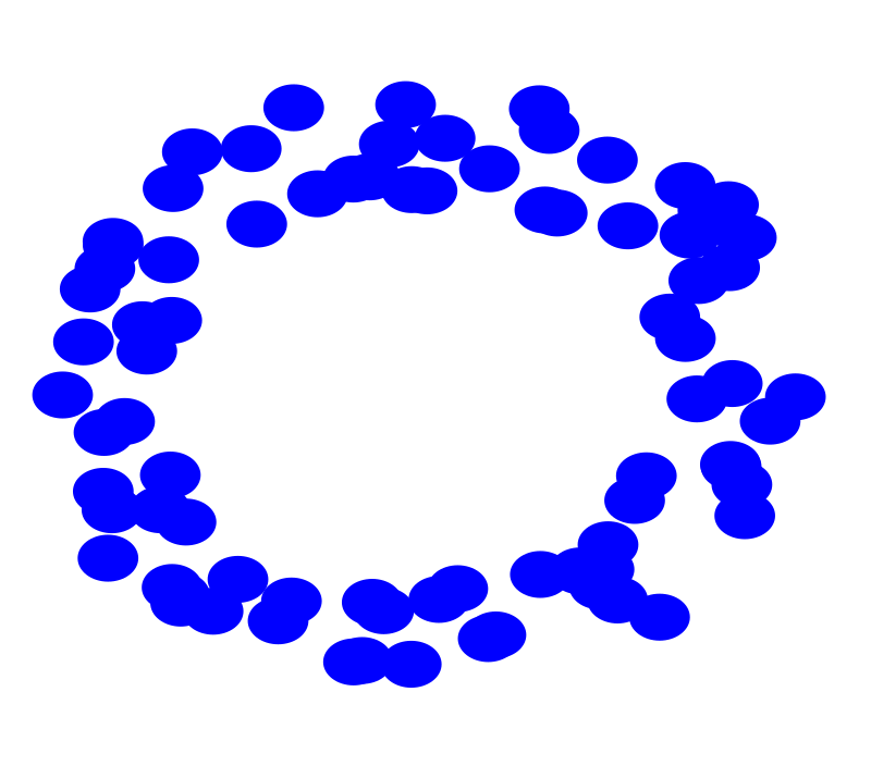
(c) $P_{2}$

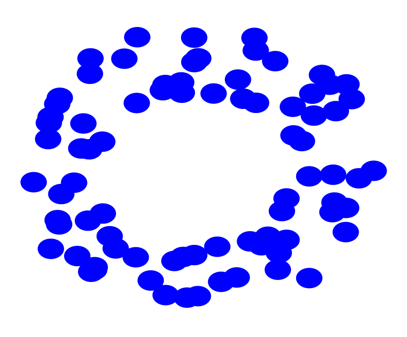
(d) $P_{3}$

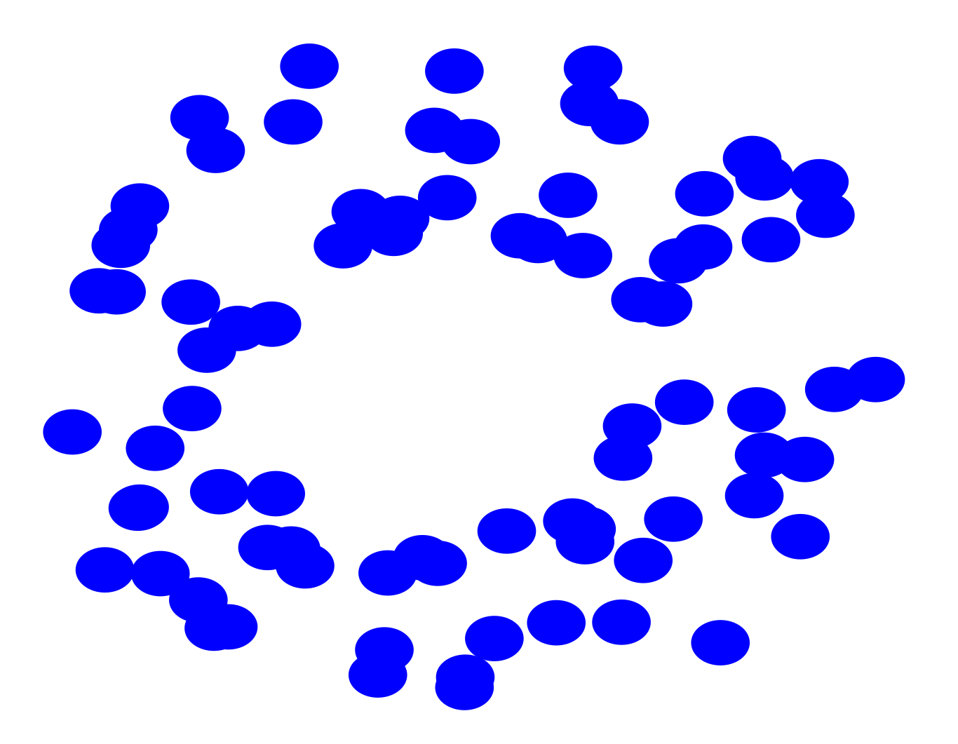
(e) $P_{4}$

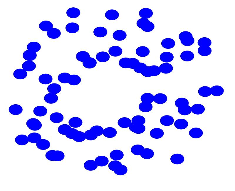
(f) $P_{5}$

Figure 18. The six point sets from Section 7.3.

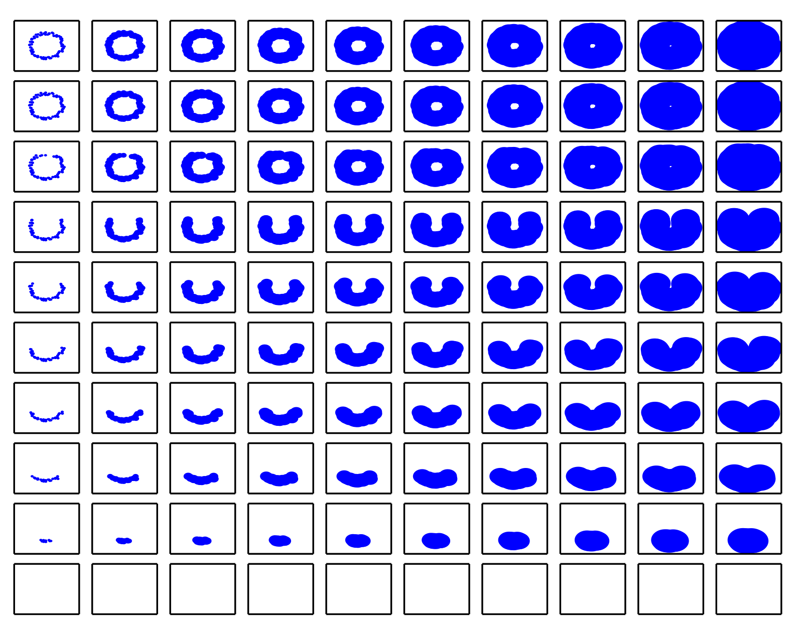
Figure 19. A bifiltration of $P_{1}$ over $G_{2}$.

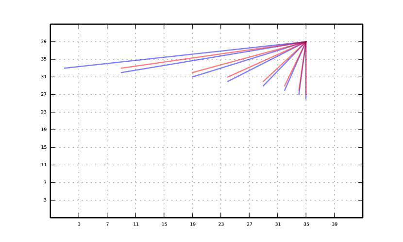
(a) $P_{0}$

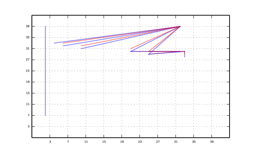
(b) $P_{1}$

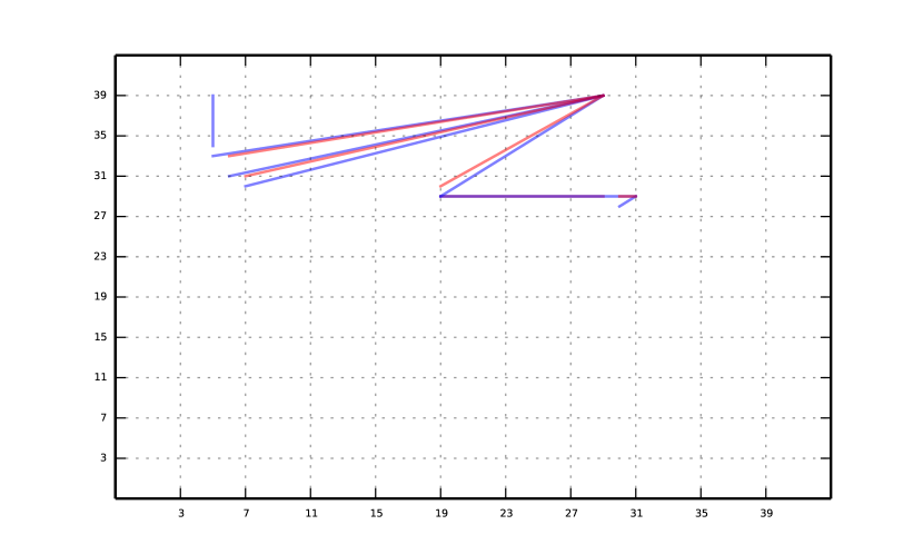
(c) $P_{2}$

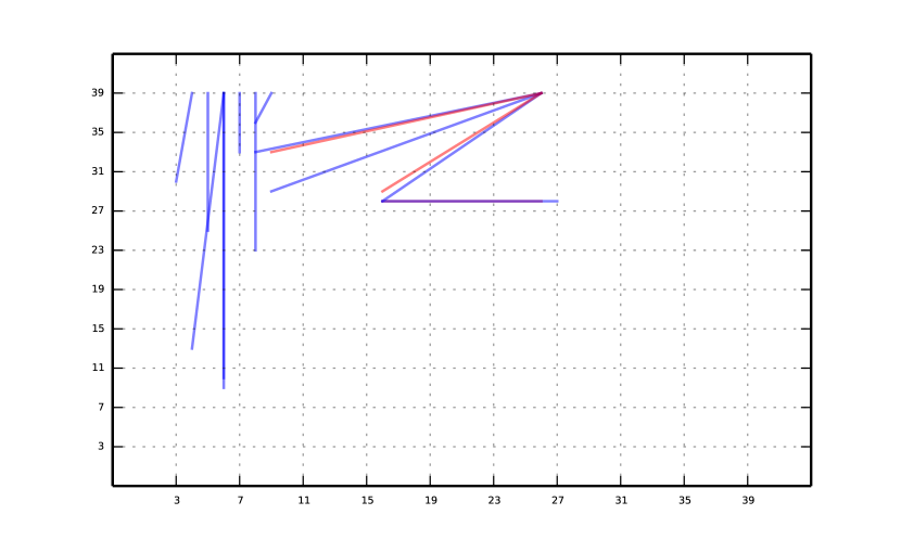
(d) $P_{3}$

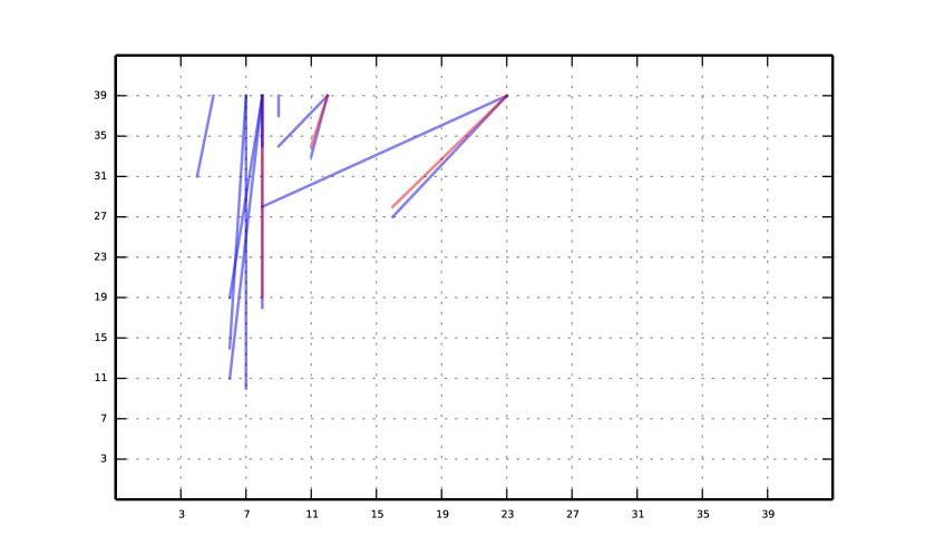
(e) $P_{4}$

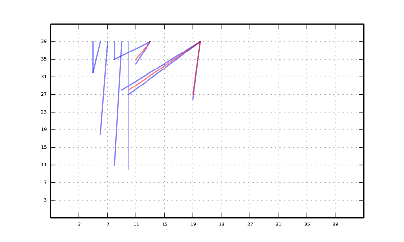
(f) $P_{5}$

Figure 20. The signed barcodes of Experiment 2 over the grid $G_{1}$ ($40\times 40)$.

7.4. Experiment 3: two-parameter clustering

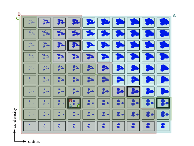
Figure 21. The bifiltration in Experiment 3. The highlighted squares show that three clusters (named A, B, C) merge in three different ways at incomparable scales. The lifespan of each one of these three clusters is marked by an interval with matching color.

• The point set $P$ consists of the $N=90$ planar points sampled from three Gaussian distributions as shown in Figure 21.

• The function $f$ is a local co-density estimate, i.e.

  $$f(p)=\#\{q\in P:d(p,q)>\epsilon\},\qquad\qquad\text{for a fixed $\epsilon\geq 0$}.$$

• The homology degree is 0 and $\mathbf{k}={\mathbb{Z}}_{2}$.

• The discretization is obtained by restriction to $G=\{r_{0},\ldots,r_{9}\}\times\{s_{0},\ldots,s_{9}\}$ — see Figure 21.

The resulting persistence module is not interval-decomposable. Geometrically, this is due to the fact that the three clusters A, B, C merge in three different ways at incomparable grades, as shown in the highlighted squares of Figure 21. Hence, one obtains the following diagram of vector spaces and linear maps:

$$\begin{gathered}\lx@xy@svg{\hbox{\raise 0.0pt\hbox{\kern 20.38889pt\hbox{\ignorespaces\ignorespaces\ignorespaces\hbox{\vtop{\kern 0.0pt\offinterlineskip\halign{\entry@#!@&&\entry@@#!@\cr\\&\\&&\crcr}}}\ignorespaces{\hbox{\kern-7.0389pt\raise 0.0pt\hbox{\hbox{\kern 0.0pt\raise 0.0pt\hbox{\hbox{\kern 3.0pt\raise 0.0pt\hbox{$\textstyle{\mathbf{k}^{2}}$}}}}}}}{\hbox{\kern-3.0pt\raise-38.74887pt\hbox{\hbox{\kern 0.0pt\raise 0.0pt\hbox{\hbox{\kern 3.0pt\raise 0.0pt\hbox{$\textstyle{}$}}}}}}}{\hbox{\kern 31.0389pt\raise-38.74887pt\hbox{\hbox{\kern 0.0pt\raise 0.0pt\hbox{\hbox{\kern 3.0pt\raise 0.0pt\hbox{$\textstyle{\mathbf{k}^{2}}$}}}}}}}{\hbox{\kern-7.0389pt\raise-77.49774pt\hbox{\hbox{\kern 0.0pt\raise 0.0pt\hbox{\hbox{\kern 3.0pt\raise 0.0pt\hbox{$\textstyle{\mathbf{k}^{3}\ignorespaces\ignorespaces\ignorespaces\ignorespaces\ignorespaces\ignorespaces\ignorespaces\ignorespaces\ignorespaces\ignorespaces\ignorespaces\ignorespaces}$}}}}}}}\ignorespaces\ignorespaces\ignorespaces\ignorespaces{}{\hbox{\lx@xy@droprule}}\ignorespaces\ignorespaces\ignorespaces{\hbox{\kern-20.38889pt\raise-34.37444pt\hbox{{}\hbox{\kern 0.0pt\raise 0.0pt\hbox{\hbox{\kern 3.0pt\hbox{\hbox{\kern 0.0pt\raise-3.63611pt\hbox{$\scriptstyle{\left[\begin{smallmatrix}1&0&0\\ 0&1&1\end{smallmatrix}\right]}$}}}\kern 3.0pt}}}}}}\ignorespaces{\hbox{\kern 0.0pt\raise-3.0pt\hbox{\hbox{\kern 0.0pt\raise 0.0pt\hbox{\lx@xy@tip{1}\lx@xy@tip{-1}}}}}}{\hbox{\lx@xy@droprule}}{\hbox{\lx@xy@droprule}}\ignorespaces\ignorespaces\ignorespaces{}\ignorespaces\ignorespaces{\hbox{\lx@xy@drawline@}}\ignorespaces\ignorespaces\ignorespaces{\hbox{\kern 21.08472pt\raise-64.2807pt\hbox{{}\hbox{\kern 0.0pt\raise 0.0pt\hbox{\hbox{\kern 3.0pt\hbox{\hbox{\kern 0.0pt\raise-3.63611pt\hbox{$\scriptstyle{\left[\begin{smallmatrix}1&1&0\\ 0&0&1\end{smallmatrix}\right]}$}}}\kern 3.0pt}}}}}}\ignorespaces{\hbox{\kern 35.13052pt\raise-41.74887pt\hbox{\hbox{\kern 0.0pt\raise 0.0pt\hbox{\lx@xy@tip{1}\lx@xy@tip{-1}}}}}}\ignorespaces\ignorespaces{\hbox{\lx@xy@drawline@}}\ignorespaces{\hbox{\lx@xy@drawline@}}\ignorespaces\ignorespaces\ignorespaces\ignorespaces{}{\hbox{\lx@xy@droprule}}\ignorespaces\ignorespaces\ignorespaces{\hbox{\kern 27.88335pt\raise-85.88385pt\hbox{{}\hbox{\kern 0.0pt\raise 0.0pt\hbox{\hbox{\kern 3.0pt\hbox{\hbox{\kern 0.0pt\raise-3.63611pt\hbox{$\scriptstyle{\left[\begin{smallmatrix}1&0&1\\ 0&1&0\end{smallmatrix}\right]}$}}}\kern 3.0pt}}}}}}\ignorespaces{\hbox{\kern 69.11668pt\raise-77.49774pt\hbox{\hbox{\kern 0.0pt\raise 0.0pt\hbox{\lx@xy@tip{1}\lx@xy@tip{-1}}}}}}{\hbox{\lx@xy@droprule}}{\hbox{\lx@xy@droprule}}{\hbox{\kern 35.07779pt\raise-77.49774pt\hbox{\hbox{\kern 0.0pt\raise 0.0pt\hbox{\hbox{\kern 3.0pt\raise 0.0pt\hbox{$\textstyle{}$}}}}}}}{\hbox{\kern 69.11668pt\raise-77.49774pt\hbox{\hbox{\kern 0.0pt\raise 0.0pt\hbox{\hbox{\kern 3.0pt\raise 0.0pt\hbox{$\textstyle{\mathbf{k}^{2}}$}}}}}}}\ignorespaces}}}}\ignorespaces\lx@xy@svg{\hbox{\raise 0.0pt\hbox{\kern 10.63885pt\hbox{\ignorespaces\ignorespaces\ignorespaces\hbox{\vtop{\kern 0.0pt\offinterlineskip\halign{\entry@#!@&&\entry@@#!@\cr\\\\}}}\ignorespaces{\hbox{\kern-3.0pt\raise 0.0pt\hbox{\hbox{\kern 0.0pt\raise 0.0pt\hbox{\hbox{\kern 3.0pt\raise 0.0pt\hbox{$\textstyle{}$}}}}}}}{\hbox{\kern-10.63885pt\raise-34.5pt\hbox{\hbox{\kern 0.0pt\raise 0.0pt\hbox{\hbox{\kern 3.0pt\raise 0.0pt\hbox{$\textstyle{\cong\ }$}}}}}}}\ignorespaces}}}}\ignorespaces\lx@xy@svg{\hbox{\raise 0.0pt\hbox{\kern 16.88889pt\hbox{\ignorespaces\ignorespaces\ignorespaces\hbox{\vtop{\kern 0.0pt\offinterlineskip\halign{\entry@#!@&&\entry@@#!@\cr\\&\\&&\crcr}}}\ignorespaces{\hbox{\kern-5.6389pt\raise 0.0pt\hbox{\hbox{\kern 0.0pt\raise 0.0pt\hbox{\hbox{\kern 3.0pt\raise 0.0pt\hbox{$\textstyle{\mathbf{k}}$}}}}}}}{\hbox{\kern-3.0pt\raise-36.94443pt\hbox{\hbox{\kern 0.0pt\raise 0.0pt\hbox{\hbox{\kern 3.0pt\raise 0.0pt\hbox{$\textstyle{}$}}}}}}}{\hbox{\kern 31.0389pt\raise-36.94443pt\hbox{\hbox{\kern 0.0pt\raise 0.0pt\hbox{\hbox{\kern 3.0pt\raise 0.0pt\hbox{$\textstyle{\mathbf{k}}$}}}}}}}{\hbox{\kern-7.0389pt\raise-74.79108pt\hbox{\hbox{\kern 0.0pt\raise 0.0pt\hbox{\hbox{\kern 3.0pt\raise 0.0pt\hbox{$\textstyle{\mathbf{k}^{2}\ignorespaces\ignorespaces\ignorespaces\ignorespaces\ignorespaces\ignorespaces\ignorespaces\ignorespaces\ignorespaces\ignorespaces\ignorespaces\ignorespaces}$}}}}}}}\ignorespaces\ignorespaces\ignorespaces\ignorespaces{}{\hbox{\lx@xy@droprule}}\ignorespaces\ignorespaces\ignorespaces{\hbox{\kern-16.88889pt\raise-33.0211pt\hbox{{}\hbox{\kern 0.0pt\raise 0.0pt\hbox{\hbox{\kern 3.0pt\hbox{\hbox{\kern 0.0pt\raise-1.75pt\hbox{$\scriptstyle{\left[\begin{smallmatrix}1&1\end{smallmatrix}\right]}$}}}\kern 3.0pt}}}}}}\ignorespaces{\hbox{\kern 0.0pt\raise-3.0pt\hbox{\hbox{\kern 0.0pt\raise 0.0pt\hbox{\lx@xy@tip{1}\lx@xy@tip{-1}}}}}}{\hbox{\lx@xy@droprule}}{\hbox{\lx@xy@droprule}}\ignorespaces\ignorespaces\ignorespaces{}\ignorespaces\ignorespaces{\hbox{\lx@xy@drawline@}}\ignorespaces\ignorespaces\ignorespaces{\hbox{\kern 20.40523pt\raise-60.03175pt\hbox{{}\hbox{\kern 0.0pt\raise 0.0pt\hbox{\hbox{\kern 3.0pt\hbox{\hbox{\kern 0.0pt\raise-1.75pt\hbox{$\scriptstyle{\left[\begin{smallmatrix}1&0\end{smallmatrix}\right]}$}}}\kern 3.0pt}}}}}}\ignorespaces{\hbox{\kern 33.77155pt\raise-39.94443pt\hbox{\hbox{\kern 0.0pt\raise 0.0pt\hbox{\lx@xy@tip{1}\lx@xy@tip{-1}}}}}}\ignorespaces\ignorespaces{\hbox{\lx@xy@drawline@}}\ignorespaces{\hbox{\lx@xy@drawline@}}\ignorespaces\ignorespaces\ignorespaces\ignorespaces{}{\hbox{\lx@xy@droprule}}\ignorespaces\ignorespaces\ignorespaces{\hbox{\kern 28.23335pt\raise-81.29108pt\hbox{{}\hbox{\kern 0.0pt\raise 0.0pt\hbox{\hbox{\kern 3.0pt\hbox{\hbox{\kern 0.0pt\raise-1.75pt\hbox{$\scriptstyle{\left[\begin{smallmatrix}0&1\end{smallmatrix}\right]}$}}}\kern 3.0pt}}}}}}\ignorespaces{\hbox{\kern 66.3167pt\raise-74.79108pt\hbox{\hbox{\kern 0.0pt\raise 0.0pt\hbox{\lx@xy@tip{1}\lx@xy@tip{-1}}}}}}{\hbox{\lx@xy@droprule}}{\hbox{\lx@xy@droprule}}{\hbox{\kern 33.6778pt\raise-74.79108pt\hbox{\hbox{\kern 0.0pt\raise 0.0pt\hbox{\hbox{\kern 3.0pt\raise 0.0pt\hbox{$\textstyle{}$}}}}}}}{\hbox{\kern 66.3167pt\raise-74.79108pt\hbox{\hbox{\kern 0.0pt\raise 0.0pt\hbox{\hbox{\kern 3.0pt\raise 0.0pt\hbox{$\textstyle{\mathbf{k}}$}}}}}}}\ignorespaces}}}}\ignorespaces\lx@xy@svg{\hbox{\raise 0.0pt\hbox{\kern 10.08331pt\hbox{\ignorespaces\ignorespaces\ignorespaces\hbox{\vtop{\kern 0.0pt\offinterlineskip\halign{\entry@#!@&&\entry@@#!@\cr\\\\}}}\ignorespaces{\hbox{\kern-3.0pt\raise 0.0pt\hbox{\hbox{\kern 0.0pt\raise 0.0pt\hbox{\hbox{\kern 3.0pt\raise 0.0pt\hbox{$\textstyle{}$}}}}}}}{\hbox{\kern-10.08331pt\raise-34.5pt\hbox{\hbox{\kern 0.0pt\raise 0.0pt\hbox{\hbox{\kern 3.0pt\raise 0.0pt\hbox{$\textstyle{\bigoplus\ }$}}}}}}}\ignorespaces}}}}\ignorespaces\lx@xy@svg{\hbox{\raise 0.0pt\hbox{\kern 9.5pt\hbox{\ignorespaces\ignorespaces\ignorespaces\hbox{\vtop{\kern 0.0pt\offinterlineskip\halign{\entry@#!@&&\entry@@#!@\cr\\&\\&&\crcr}}}\ignorespaces{\hbox{\kern-5.6389pt\raise 0.0pt\hbox{\hbox{\kern 0.0pt\raise 0.0pt\hbox{\hbox{\kern 3.0pt\raise 0.0pt\hbox{$\textstyle{\mathbf{k}}$}}}}}}}{\hbox{\kern-3.0pt\raise-36.94443pt\hbox{\hbox{\kern 0.0pt\raise 0.0pt\hbox{\hbox{\kern 3.0pt\raise 0.0pt\hbox{$\textstyle{}$}}}}}}}{\hbox{\kern 29.6389pt\raise-36.94443pt\hbox{\hbox{\kern 0.0pt\raise 0.0pt\hbox{\hbox{\kern 3.0pt\raise 0.0pt\hbox{$\textstyle{\mathbf{k}}$}}}}}}}{\hbox{\kern-5.6389pt\raise-73.88885pt\hbox{\hbox{\kern 0.0pt\raise 0.0pt\hbox{\hbox{\kern 3.0pt\raise 0.0pt\hbox{$\textstyle{\mathbf{k}\ignorespaces\ignorespaces\ignorespaces\ignorespaces\ignorespaces\ignorespaces\ignorespaces\ignorespaces\ignorespaces\ignorespaces\ignorespaces\ignorespaces}$}}}}}}}\ignorespaces\ignorespaces\ignorespaces\ignorespaces{}{\hbox{\lx@xy@droprule}}\ignorespaces\ignorespaces\ignorespaces{\hbox{\kern-9.5pt\raise-33.47221pt\hbox{{}\hbox{\kern 0.0pt\raise 0.0pt\hbox{\hbox{\kern 3.0pt\hbox{\hbox{\kern 0.0pt\raise-2.25555pt\hbox{$\scriptstyle{1}$}}}\kern 3.0pt}}}}}}\ignorespaces{\hbox{\kern 0.0pt\raise-3.0pt\hbox{\hbox{\kern 0.0pt\raise 0.0pt\hbox{\lx@xy@tip{1}\lx@xy@tip{-1}}}}}}{\hbox{\lx@xy@droprule}}{\hbox{\lx@xy@droprule}}\ignorespaces\ignorespaces\ignorespaces{}\ignorespaces\ignorespaces{\hbox{\lx@xy@drawline@}}\ignorespaces\ignorespaces\ignorespaces{\hbox{\kern 19.02573pt\raise-58.98451pt\hbox{{}\hbox{\kern 0.0pt\raise 0.0pt\hbox{\hbox{\kern 3.0pt\hbox{\hbox{\kern 0.0pt\raise-2.25555pt\hbox{$\scriptstyle{1}$}}}\kern 3.0pt}}}}}}\ignorespaces{\hbox{\kern 32.41257pt\raise-39.94443pt\hbox{\hbox{\kern 0.0pt\raise 0.0pt\hbox{\lx@xy@tip{1}\lx@xy@tip{-1}}}}}}\ignorespaces\ignorespaces{\hbox{\lx@xy@drawline@}}\ignorespaces{\hbox{\lx@xy@drawline@}}\ignorespaces\ignorespaces\ignorespaces\ignorespaces{}{\hbox{\lx@xy@droprule}}\ignorespaces\ignorespaces\ignorespaces{\hbox{\kern 30.5278pt\raise-79.14441pt\hbox{{}\hbox{\kern 0.0pt\raise 0.0pt\hbox{\hbox{\kern 3.0pt\hbox{\hbox{\kern 0.0pt\raise-2.25555pt\hbox{$\scriptstyle{1}$}}}\kern 3.0pt}}}}}}\ignorespaces{\hbox{\kern 64.9167pt\raise-73.88885pt\hbox{\hbox{\kern 0.0pt\raise 0.0pt\hbox{\lx@xy@tip{1}\lx@xy@tip{-1}}}}}}{\hbox{\lx@xy@droprule}}{\hbox{\lx@xy@droprule}}{\hbox{\kern 32.2778pt\raise-73.88885pt\hbox{\hbox{\kern 0.0pt\raise 0.0pt\hbox{\hbox{\kern 3.0pt\raise 0.0pt\hbox{$\textstyle{}$}}}}}}}{\hbox{\kern 64.9167pt\raise-73.88885pt\hbox{\hbox{\kern 0.0pt\raise 0.0pt\hbox{\hbox{\kern 3.0pt\raise 0.0pt\hbox{$\textstyle{\mathbf{k}}$}}}}}}}\ignorespaces}}}}\ignorespaces\end{gathered} \textstyle{\mathbf{k}^{2}} \textstyle{\mathbf{k}^{2}} \textstyle{\mathbf{k}^{3}\ignorespaces\ignorespaces\ignorespaces\ignorespaces\ignorespaces\ignorespaces\ignorespaces\ignorespaces\ignorespaces\ignorespaces\ignorespaces\ignorespaces} \scriptstyle{\left[\begin{smallmatrix}1&0&0\\ 0&1&1\end{smallmatrix}\right]} \scriptstyle{\left[\begin{smallmatrix}1&1&0\\ 0&0&1\end{smallmatrix}\right]} \scriptstyle{\left[\begin{smallmatrix}1&0&1\\ 0&1&0\end{smallmatrix}\right]} \textstyle{\mathbf{k}^{2}} \textstyle{\cong\ } \textstyle{\mathbf{k}} \textstyle{\mathbf{k}} \textstyle{\mathbf{k}^{2}\ignorespaces\ignorespaces\ignorespaces\ignorespaces\ignorespaces\ignorespaces\ignorespaces\ignorespaces\ignorespaces\ignorespaces\ignorespaces\ignorespaces} \scriptstyle{\left[\begin{smallmatrix}1&1\end{smallmatrix}\right]} \scriptstyle{\left[\begin{smallmatrix}1&0\end{smallmatrix}\right]} \scriptstyle{\left[\begin{smallmatrix}0&1\end{smallmatrix}\right]} \textstyle{\mathbf{k}} \textstyle{\bigoplus\ } \textstyle{\mathbf{k}} \textstyle{\mathbf{k}} \textstyle{\mathbf{k}\ignorespaces\ignorespaces\ignorespaces\ignorespaces\ignorespaces\ignorespaces\ignorespaces\ignorespaces\ignorespaces\ignorespaces\ignorespaces\ignorespaces} \scriptstyle{1} \scriptstyle{1} \scriptstyle{1} \textstyle{\mathbf{k}} \textstyle{\mathbf{k}^{2}} \textstyle{\mathbf{k}^{2}} \textstyle{\mathbf{k}^{3}\ignorespaces\ignorespaces\ignorespaces\ignorespaces\ignorespaces\ignorespaces\ignorespaces\ignorespaces\ignorespaces\ignorespaces\ignorespaces\ignorespaces} \scriptstyle{\left[\begin{smallmatrix}1&0&0\\ 0&1&1\end{smallmatrix}\right]} \scriptstyle{\left[\begin{smallmatrix}1&1&0\\ 0&0&1\end{smallmatrix}\right]} \scriptstyle{\left[\begin{smallmatrix}1&0&1\\ 0&1&0\end{smallmatrix}\right]} \textstyle{\mathbf{k}^{2}} \textstyle{\cong\ } \textstyle{\mathbf{k}} \textstyle{\mathbf{k}} \textstyle{\mathbf{k}^{2}\ignorespaces\ignorespaces\ignorespaces\ignorespaces\ignorespaces\ignorespaces\ignorespaces\ignorespaces\ignorespaces\ignorespaces\ignorespaces\ignorespaces} \scriptstyle{\left[\begin{smallmatrix}1&1\end{smallmatrix}\right]} \scriptstyle{\left[\begin{smallmatrix}1&0\end{smallmatrix}\right]} \scriptstyle{\left[\begin{smallmatrix}0&1\end{smallmatrix}\right]} \textstyle{\mathbf{k}} \textstyle{\bigoplus\ } \textstyle{\mathbf{k}} \textstyle{\mathbf{k}} \textstyle{\mathbf{k}\ignorespaces\ignorespaces\ignorespaces\ignorespaces\ignorespaces\ignorespaces\ignorespaces\ignorespaces\ignorespaces\ignorespaces\ignorespaces\ignorespaces} \scriptstyle{1} \scriptstyle{1} \scriptstyle{1} \textstyle{\mathbf{k}}$$

The obtained signed barcode and prominence diagram are shown in Figure 22. As expected, the lifespans of the three clusters A, B, C appear as three separate subsets of the bars, as shown in Figure 23. Moreover, these three subsets of bars can be discriminated from the rest of the barcode by their prominence, as seen from the prominence diagram. Checking whether any one of these three subsets of bars does correspond to the lifespan of some feature can then be done by computing the coefficient assigned to the corresponding interval in the minimal generalized rank decomposition of $M$.

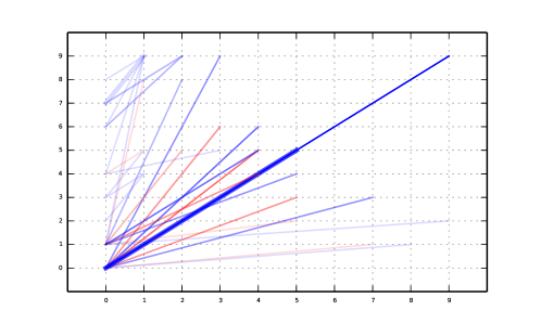
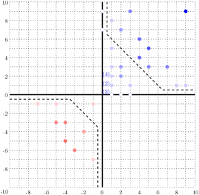
Figure 22. Left: signed barcode of Experiment 3 over the $10\times 10$ grid. Thicker bars overlap with another bar. Right: corresponding prominence diagram, where the bars coming from the lifespans of $A,B,C$ are separated from the rest of the bars by the dashed curves. Each bar with endpoints $s\leq t$ in the barcode (and diagram) has an intensity proportional to $\min\{t_{x}-s_{x},\,t_{y}-s_{y}\}$; in particular, horizontal and vertical bars are invisible.

Figure 23. Lifespans of $A,B$ (left) and $C$ (right) in the signed barcode.

8. Discussion

We conclude the paper by further discussing some aspects of our work and the prospects they raise.

Generalized rank-exact resolutions

Considering short exact sequences on which rank is additive is more subtle when we consider generalized ranks. The following example shows that in general we cannot expect to obtain an exact structure in this way.

Example 8.1.

Consider the $2\times 2$-grid, and the interval ${I}$ indicated below.

For this grid all indecomposables are thin, and we will denote them by their dimension vectors. Consider the following commutative diagram with exact rows.

Here the middle vertical arrow is the projection to the first summand. Note that $\operatorname{Rk}_{{I}}$ is zero on all objects in this diagram, except the right upper corner, where it is one. In particular $\operatorname{Rk}_{I}$ is additive on the lower sequence, but not on the upper one. But the upper sequence is a pull-back of the lower one. This shows that the collection of short exact sequences such that $\operatorname{Rk}_{{I}}$ is additive does not constitute an exact structure.

About the collection $\mathcal{I}$ of intervals involved in the rank decompositions

In Definition 1.4 and throughout the paper, we have been enforcing the collection $\mathcal{I}$ of intervals involved in the generalized rank invariant to be the same as the collection from which intervals are picked for the rank decompositions. Thus, $\mathcal{I}$ has played a double role:

• that of a test set of shapes over which the existence of “features” is being probed by the (generalized) rank invariant;

• that of a dictionary of shapes (formally, a basis of rank functions) over which the rank decompositions are built.

It is natural to try decorrelating the two roles by assigning a different collection of intervals to each one of them, say $\mathcal{I}_{t}$ for the test set and $\mathcal{I}_{d}$ for the dictionary. The problem becomes then to decompose (generalized) rank invariants $\operatorname{Rk}_{\mathcal{I}_{t}}M$, or more generally, to decompose maps $r:\mathcal{I}_{t}\to{\mathbb{Z}}$, over the family of rank invariants $\left(\operatorname{Rk}_{\mathcal{I}_{t}}\mathbf{k}_{R}\right)_{{R}\in\mathcal{I}_{d}}$. As we have set $\mathcal{I}_{t}=\mathcal{I}_{d}$ so far, the question is what happens when either $\mathcal{I}_{t}\supsetneq\mathcal{I}_{d}$ or $\mathcal{I}_{t}\subsetneq\mathcal{I}_{d}$.

Letting $\mathcal{I}_{t}\supsetneq\mathcal{I}_{d}$ seems pointless, since the corresponding minimal decompositions are still unique and correspond de facto to the ones obtained with $\mathcal{I}_{d}=\mathcal{I}_{t}$, if they exist at all, thus bringing no further insight.

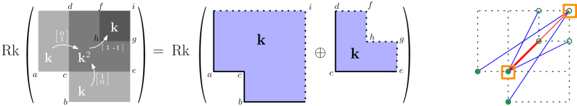
Figure 24. Left and center: one of several possible minimal rank decompositions, over the collection of all intervals of ${\mathbb{R}}^{2}$, of the usual rank invariant of the finitely-presented module $M$ from Figure 8. Right: the corresponding decorated signed barcode, where the orange squares indicate how the bars are clustered into two groups coming from the two elements in the decomposition at the center (note: the bottom-left orange square does not include the longer red bar).

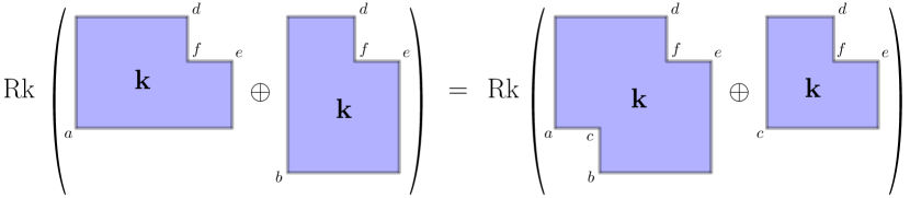
Figure 25. Two interval-decomposable modules with the same usual rank invariant. The module on the right-hand side is one among several possible minimal usual rank decompositions of the module on the left-hand side over the full collection of intervals of ${\mathbb{R}}^{2}$. Notice how this decomposition creates the illusion that a feature spans the entire interval with perimeter $(a,c,b,e,f,d)$, whereas no such feature actually exists in the module on the left-hand side.

By contrast, letting $\mathcal{I}_{t}\subsetneq\mathcal{I}_{d}$ seems a better idea. Indeed, by enlarging the dictionary, one may possibly obtain smaller minimal rank decompositions, whose elements carry more structure individually than the shapes in $\mathcal{I}_{t}$ do. Examples are given in Figures 2 and 24, where the test set only contains the rectangles while the dictionary includes all the intervals in the plane. In practice, finding the right trade-off between simplifying the decomposition and complexifying the individual structure of the shapes in the dictionary is key. Moreover, an important caveat in this setting is that the uniqueness of the minimal decomposition (in which $\mathcal{R}$ and $\mathcal{S}$ are disjoint as multi-sets) will usually be lost: for instance, the rank decompositions from Figures 2 and 3 are valid minimal rank decompositions over the test set $\mathcal{I}_{t}$ composed of the rectangles in the $3\times 3$ grid, nevertheless they are distinct. Thus, rank decompositions are no longer canonically defined, which is a fundamental limitation in practice when interpretation or comparison of poset representations is at stake. An illustration is given in Figure 25, where the use of an inappropriate minimal decomposition creates the illusion that there is a “feature” that persists over a certain interval whereas no such feature actually exists in the original poset representation.

These considerations justify our choice of letting $\mathcal{I}_{t}=\mathcal{I}_{d}$ in Definition 1.4 and throughout our analysis. Yet, at this stage we are leaving open the possibility of using a larger dictionary than the test set, acknowledging that, in some specific applications, it may be useful to have a larger dictionary of shapes on which to interpret the structure of the rank invariant.

Limitations of rank decompositions

As rank decompositions encode the structure of rank invariants, they are just as powerful descriptors as the rank invariants themselves. In particular, they are not complete descriptors for multi-parameter persistence modules nor, more generally, for poset representations. For instance, we see from Figure 5 that the direct sum of the indecomposable module on the left-hand side of the figure with the red module on the right-hand side has the same generalized ranks as the blue module in that same figure. As a consequence, they are indistinguishable from each other based solely on their generalized rank invariants. An important question that comes up is how much of the structure of a persistence module may be missed by these descriptors.

If we restrict our focus to interval-decomposable representations over finite posets, then we know from Proposition 2.10 that the generalized rank invariant (with $\mathcal{I}$ being the full collection of intervals in the poset) is a complete descriptor, therefore so is its minimal rank decomposition. Of course, the usual rank invariant itself is not a complete descriptor, as illustrated in Figure 25, however it is complete on the subcategory of interval representations—where the interval support of each object is fully characterized by the support of its usual rank invariant. An important question in practice is how to choose the collection $\mathcal{I}$ of intervals, between the collection of closed segments (which corresponds to taking the usual rank invariant) and the full collection of intervals in the poset, to find the right trade-off between the richness of the invariant and the complexity of its calculation.

Signed barcodes versus RIVET

As explained in Section 6, signed barcodes play a role similar to that of classical barcodes in one-parameter persistence: they carry information about the global structure of the rank invariant, and they allow for certain visually-enabled procedures to retrieve the value of the rank invariant at indices $s\leq t$, or the barcodes of the restriction of the module to a given strictly monotone line. Thus, they appear as a viable alternative to RIVET [25] for the exploration of multi-parameter persistence modules. They can also be used in conjunction with RIVET, or parts thereof, for instance: using RIVET to compute minimal presentations, then using the dynamic programming procedure from [7] to compute the usual rank invariant, and finally using (5.1) to compute the corresponding minimal rank decomposition and signed barcode.

Unlike RIVET, signed barcodes are readily available for persistence modules with an arbitrary number of parameters. They are easy to compute once the usual rank invariant has been computed, and in the two-parameter case the total running time compares favorably to that of RIVET—see Remark 5.3. They are also easy to encode, and their storage size never exceeds that of the usual rank invariant (since there are no more distinct rectangles $\langle s,t\rangle$ than there are pairs of comparable indices $s\leq t$ in the input filtration). On the downside, for now there still remains work to be done—out of the scope of this paper—to design a corresponding data structure that allows for efficient (logarithmic-time) queries as in RIVET.

Statistics and machine learning with signed barcodes

While we have been mainly discussing the interpretability of our rank decompositions via their associated signed barcodes, motivated by the exploration of multi-parameter persistence modules, we should recall that, in the one-parameter setting, barcodes are also used to extract features from data, with applications in machine learning and artificial intelligence. To this end, a number of vectorizations and kernels for (unsigned) barcodes have been proposed—see e.g. [1, 8, 11, 21, 23, 30], the vast majority of which enjoy stability properties in terms of the bottleneck distance between barcodes. Here, considering the nature of the signed barcodes, and the (pseudo-)distance put on their corresponding rank decompositions in Section 5.4, it is possible that a subset of these techniques adapts naturally, with similar stability guarantees following from Theorem 5.9. Meanwhile, the decorations that can be put on the signed barcodes, to encode generalized rank invariants, may be a valuable added piece of information in practice, which raises the question of finding the most appropriate way to include these decorations in the constructions of the vectorizations or kernels. It will then be interesting to compare the outcome, both in terms of performances in machine learning applications and in terms of computation time, to previous vectorizations or kernels for multi-parameter persistence modules [10, 14, 32]. The key point is that these previous techniques essentially slice the input module by arbitrarily chosen collections of lines, and aggregate the resulting fibered barcodes—either by concatenation, by integration, or through vineyards; the added value of the signed barcode is to provide insight into which lines are most relevant for the slicing, potentially allowing for faster and more accurate computations, producing both richer and smaller-sized features.

The metric space of rank decompositions may also be in itself a relevant object of study. An obvious question is whether the matching distance between rank decompositions can be translated into an optimal transportation distance between signed barcodes, possibly up to some constants. If the answer is positive, then, similarly to the space of unsigned barcodes in one-parameter persistence, the space of signed barcodes in multi-parameter persistence will be comparable to a space of (signed) measures, and the techniques developed in the one-parameter setting for doing statistics with unsigned barcodes may be adapted to work with signed barcodes as well. Meanwhile, the computation of the metric between rank decompositions will be greatly facilitated by its translation into a combinatorial matching problem—currently the signed barcodes provide insight into the structure of each individual rank decomposition and its corresponding rank invariant, however it is still unknown how to exploit this knowledge to find the most relevant directions for the matching distance between rank decompositions.

References

- [1] H. Adams, T. Emerson, M. Kirby, R. Neville, C. Peterson, P. Shipman, S. Chepushtanova, E. Hanson, F. Motta, and L. Ziegelmeier. Persistence images: A stable vector representation of persistent homology. Journal of Machine Learning Research, 18, 2017.
- [2] H. Asashiba, E. G. Escolar, K. Nakashima, and M. Yoshiwaki. On approximation of 2d persistence modules by interval-decomposables. arXiv preprint arXiv:1911.01637, 2019.
- [3] M. Auslander and Ø. Solberg. Relative homology and representation theory 1: Reative homology and homologically finite subcategories. Communications in Algebra, 21(9):2995–3031, 1993.
- [4] L. Betthauser, P. Bubenik, and P. B. Edwards. Graded persistence diagrams and persistence landscapes. Discrete & Computational Geometry, 67(1):203–230, 2022.
- [5] B. Blanchette, T. Brüstle, and E. J. Hanson. Homological approximations in persistence theory. arXiv preprint arXiv:2112.07632, 2021.
- [6] M. Botnan and W. Crawley-Boevey. Decomposition of persistence modules. Proceedings of the American Mathematical Society, 148(11):4581–4596, 2020.
- [7] M. B. Botnan, V. Lebovici, and S. Oudot. On Rectangle-Decomposable 2-Parameter Persistence Modules. In S. Cabello and D. Z. Chen, editors, 36th International Symposium on Computational Geometry (SoCG 2020), volume 164 of Leibniz International Proceedings in Informatics (LIPIcs), pages 22:1–22:16, Dagstuhl, Germany, 2020. Schloss Dagstuhl–Leibniz-Zentrum für Informatik.
- [8] P. Bubenik. Statistical topological data analysis using persistence landscapes. J. Mach. Learn. Res., 16(1):77–102, 2015.
- [9] T. Bühler. Exact categories. Expositiones Mathematicae, 28(1):1–69, 2010.
- [10] M. Carrier̀e and A. Blumberg. Multiparameter persistence image for topological machine learning. In H. Larochelle, M. Ranzato, R. Hadsell, M. F. Balcan, and H. Lin, editors, Advances in Neural Information Processing Systems, volume 33, pages 22432–22444. Curran Associates, Inc., 2020.
- [11] M. Carriere, M. Cuturi, and S. Oudot. Sliced wasserstein kernel for persistence diagrams. In International Conference on Machine Learning, pages 664–673. PMLR, 2017.
- [12] F. Chazal, V. De Silva, M. Glisse, and S. Oudot. The structure and stability of persistence modules. Springer, 2016.
- [13] D. Cohen-Steiner, H. Edelsbrunner, and J. Harer. Stability of persistence diagrams. Discrete & Computational Geometry, 37(1):103–120, 2007.
- [14] R. Corbet, U. Fugacci, M. Kerber, C. Landi, and B. Wang. A kernel for multi-parameter persistent homology. Computers & graphics: X, 2:100005, 2019.
- [15] W. Crawley-Boevey. Decomposition of pointwise finite-dimensional persistence modules. Journal of Algebra and its Applications, 14(05):1550066, 2015.
- [16] T. K. Dey and C. Xin. Generalized persistence algorithm for decomposing multi-parameter persistence modules. arXiv preprint arXiv:1904.03766, 2019.
- [17] P. Dräxler, I. Reiten, S. Smalø, Ø. Solberg, B. Keller, et al. Exact categories and vector space categories. Transactions of the American Mathematical Society, 351(2):647–682, 1999.
- [18] H. Edelsbrunner, D. Letscher, and A. Zomorodian. Topological persistence and simplification. Discrete Comput. Geom., 28:511–533, 2002.
- [19] A. Heller. Homological algebra in abelian categories. Ann. of Math. (2), 68:484–525, 1958.
- [20] W. Kim and F. Memoli. Generalized persistence diagrams for persistence modules over posets. arXiv preprint arXiv:1810.11517, 2018.
- [21] G. Kusano, Y. Hiraoka, and K. Fukumizu. Persistence weighted gaussian kernel for topological data analysis. In International Conference on Machine Learning, pages 2004–2013. PMLR, 2016.
- [22] C. Landi. The rank invariant stability via interleavings. In Research in computational topology, pages 1–10. Springer, 2018.
- [23] T. Le and M. Yamada. Persistence fisher kernel: A riemannian manifold kernel for persistence diagrams. In Proceedings of the 32nd International Conference on Neural Information Processing Systems, NIPS’18, page 10028–10039, Red Hook, NY, USA, 2018. Curran Associates Inc.
- [24] M. Lesnick. The theory of the interleaving distance on multidimensional persistence modules. Foundations of Computational Mathematics, 15(3):613–650, 2015.
- [25] M. Lesnick and M. Wright. Interactive visualization of 2-d persistence modules. arXiv preprint arXiv:1512.00180, 2015.
- [26] A. McCleary and A. Patel. Edit distance and persistence diagrams over lattices, 2021.
- [27] N. Milosavljević, D. Morozov, and P. Skraba. Zigzag persistent homology in matrix multiplication time. In Proceedings of the twenty-seventh annual symposium on Computational geometry, pages 216–225. ACM, 2011.
- [28] A. Patel. Generalized persistence diagrams. Journal of Applied and Computational Topology, 1(3):397–419, 2018.
- [29] D. Quillen. Higher algebraic -theory. I. In Algebraic -theory, I: Higher -theories (Proc. Conf., Battelle Memorial Inst., Seattle, Wash., 1972), pages 85–147. Lecture Notes in Math., Vol. 341, 1973.
- [30] J. Reininghaus, S. Huber, U. Bauer, and R. Kwitt. A stable multi-scale kernel for topological machine learning. In Proceedings of the IEEE conference on computer vision and pattern recognition, pages 4741–4748, 2015.
- [31] G.-C. Rota. On the foundations of combinatorial theory i. theory of möbius functions. Zeitschrift für Wahrscheinlichkeitstheorie und verwandte Gebiete, 2(4):340–368, 1964.
- [32] O. Vipond. Multiparameter persistence landscapes. Journal of Machine Learning Research, 21(61):1–38, 2020.
- [33] A. Zomorodian and G. Carlsson. Computing persistent homology. Discrete & Computational Geometry, 33(2):249–274, 2005.