MiNNLO_PS: a new method to match NNLO QCD with parton showers

Abstract

I describe MiNNLO_PS, a novel method to match NNLO QCD computations with Parton Showers, and present a selection of results for color-singlet production at the LHC.

1 Introduction

The current experimental precision reached by the LHC experimental collaborations (and even more the future prospects) requires theoretical predictions whose formal accuracy go beyond the computation of NLO QCD corrections and their matching to parton showers (NLO+PS). Adding (N)NNLO QCD corrections, and NLO EW ones (or combination thereof), is crucial, as often it is only through such predictions that a comparison between data and theory is made possible without being limited by large theoretical uncertainties, or by missing shapes and normalization effects due to NNLO QCD and NLO EW corrections. Nowadays the NNLO QCD corrections to essentially all the $2\to 2$ processes  at the LHC are known, and NLO EW corrections can be computed also for process with spectacularly high multiplicity ($2\to 8$).

It is known that, in the corners of phase space where an hierarchy between two or more scales develop, fixed-order QCD predictions fail, due to the presence of large logarithms, that need to be resummed to all orders. The recent progress in this field has been remarkable as well, not only due to the extremely precise predictions obtained for specific observables (in some cases, N³LL^′), but also because of the development of parton-shower algorithms whose logarithmic accuracy can be formally established for a wide class of observables, and systematically improved.

A fully-differential Monte Carlo event generator that incorporates, consistently, several of the above developments does not exist yet. Nevertheless, the issue of matching NNLO QCD corrections to PS has been already addressed by different groups, and NNLO+PS results have been obtained with four methods: “reweighted MiNLO^′” [1, 2], Geneva [3, 4], Unnlops [5], MiNNLO_PS [6, 7]. All the processes with 2 massless colored legs at LO can be described with this accuracy, and many results have been already obtained [2, 10, 11, 12, 13, 14, 19, 20, 21, 22, 23, 24, 25, 5, 17, 18, 6, 7, 15, 16, 26].

In this contribution, I present MiNNLO_PS [6, 7], a new method to match NNLO QCD computations with parton showers. I focus on color-singlet production processes, although the method I describe has been already successfully extended to deal with a colored and massive final state, and used to simulate top-pair production at NNLO+PS accuracy, obtaining, for the first time, a NNLO+PS result for a process with more than two colored legs at LO [8] .

Denoting with $F$ the color-singlet final state, and with $p_{t}$ its transverse momentum, the requirements of NNLO+PS prediction are:

• NNLO accuracy for observables that are inclusive on radiation (e.g. $d\sigma/dy_{F}$).

• NLO(LO) accuracy for $F+1$$(2)$ jet observables in the hard region (e.g. $d\sigma/dp_{t,j}$), possibly with a scale choice that is appropriate for each kinematic regime.

• Resummation of soft/collinear logarithms where relevant (e.g. $\sigma(p_{t,j}<p_{t,veto})$ or $d\sigma/dp_{t}$).

The formal logarithmic accuracy that can be obtained by NNLO+PS methods for specific observables is currently an open question. As far as this manuscript is concerned, I will just assume that a NNLO+PS prediction must preserve the logarithmic accuracy of the PS, that I will assume to be leading-logarithmic (LL). Theoretical ideas that already go beyond the NNLO+PS requirements outlined above exist as well [27, 28].

2 The MiNNLO_PS method

2.1 MiNNLO_PS in a nutshell

From $p_{t}$-resummation techniques  one can show that the differential cross-section for $F+X$ production can be written as

$$\frac{\mathrm{d}\sigma}{\mathrm{d}p_{t}\mathrm{d}\Phi_{\scriptscriptstyle\rm F}}=\frac{\mathrm{d}}{\mathrm{d}p_{t}}\Big{\{}\mathcal{L}(\Phi_{\rm F},p_{t})\exp[-\tilde{S}(p_{t})]\Big{\}}+R_{\rm finite}(p_{t})\,,$$ (1)

where the luminosity $\mathcal{L}(\Phi_{\scriptscriptstyle\rm F},p_{t})$ contains the hard virtual corrections and the coefficient functions for $F$ production (expanded in powers of $\alpha_{\scriptscriptstyle\rm S}(p_{t})$), $\exp[-\tilde{S}(p_{t})]$ is the Sudakov form factor for the (direct-space) resummation of logarithms $\log(Q/p_{t})$, and $R_{\rm finite}(p_{t})$ is the finite part of the $F+1$ jet differential cross section $\mathrm{d}\sigma_{\scriptscriptstyle\rm FJ}/\mathrm{d}\Phi_{\scriptscriptstyle\rm FJ}$. If $\mathcal{L}$ contains the hard-virtual and the collinear coefficient functions up to second order in $\alpha_{\scriptscriptstyle\rm S}(p_{t})$, and $R_{\rm finite}(p_{t})$ is NLO accurate in the $p_{t}$ spectrum, the integral over $p_{t}$ of Eq. 1 yields NNLO accurate results for $F$ production. The MiNNLO_PS method relies on the observation that, after neglecting terms that, upon integration in $p_{t}$, give contributions beyond the required accuracy, Eq. 1 can be recast to a form that matches the POWHEG $\bar{B}$ function for the process $F+1$ jet:

$$\frac{\mathrm{d}\bar{B}(\Phi_{\scriptscriptstyle\rm FJ})}{\mathrm{d}\Phi_{\scriptscriptstyle\rm FJ}} = \exp[-\tilde{S}(p_{t})]\bigg{\{}{\frac{\alpha_{\scriptscriptstyle\rm S}(p_{t})}{2\pi}\left[\frac{\mathrm{d}\sigma_{\scriptscriptstyle\rm FJ}}{\mathrm{d}\Phi_{\scriptscriptstyle\rm FJ}}\right]^{(1)}\left(1+\frac{\alpha_{\scriptscriptstyle\rm S}(p_{t})}{2\pi}[\tilde{S}(p_{t})]^{(1)}\right)}$$ (2)

$${+\left(\frac{\alpha_{\scriptscriptstyle\rm S}(p_{t})}{2\pi}\right)^{2}\left[\frac{\mathrm{d}\sigma_{\scriptscriptstyle\rm FJ}}{\mathrm{d}\Phi_{\scriptscriptstyle\rm FJ}}\right]^{(2)}}+{\left(\frac{\alpha_{\scriptscriptstyle\rm S}(p_{t})}{2\pi}\right)^{3}[D(\Phi_{\scriptscriptstyle\rm F},p_{t})]^{(3)}{F^{\scriptscriptstyle\rm{corr}}(\Phi_{\scriptscriptstyle\rm FJ})}}\bigg{\}}\,,$$

where

$$D(\Phi_{\scriptscriptstyle\rm F},p_{t})=-\frac{\mathrm{d}\tilde{S}(p_{t})}{\mathrm{d}p_{t}}{\cal L}(\Phi_{\scriptscriptstyle\rm F},p_{t})+\frac{\mathrm{d}{\cal L}(\Phi_{\scriptscriptstyle\rm F},p_{t})}{\mathrm{d}p_{t}}\,,$$ (3)

and $[X]^{(k)}$ is defined by $X=\sum_{k}(\frac{\alpha_{\scriptscriptstyle\rm S}}{2\pi})^{k}[X]^{(k)}$.

In Eq. 2 one recognizes the MiNLO^′ formula, and the extra term $[D(p_{t})]^{(3)}$ needed to get NNLO accuracy. As $D$ is extracted from equations valid in the $p_{t}\to 0$ limit, it formally depends on $(\Phi_{\scriptscriptstyle\rm F},p_{t})$: in order to obtain the final expression of Eq. 2 for an improved $\bar{B}$ function that depends, instead, on $\Phi_{\scriptscriptstyle\rm FJ}$, one needs to introduce a smooth mapping and a projection $F^{\scriptscriptstyle\rm{corr}}(\Phi_{\scriptscriptstyle\rm FJ})$, so that, when integrating the $DF$ term in Eq. 2 over $\Phi_{\scriptscriptstyle\rm FJ}$ at fixed $(\Phi_{\scriptscriptstyle\rm F},p_{t})$, one recovers exactly $D(\Phi_{\scriptscriptstyle\rm F},p_{t})$.

Truncating $D$ at the third order is formally correct, and it is the approach used in ref. [6], although by keeping its full expression, i.e.

$$\left(\frac{\alpha_{\scriptscriptstyle\rm S}(p_{t})}{2\pi}\right)^{3}[D(p_{t})]^{(3)}\to D-\frac{\alpha_{\scriptscriptstyle\rm S}(p_{t})}{2\pi}[D(p_{t})]^{(1)}-\left(\frac{\alpha_{\scriptscriptstyle\rm S}(p_{t})}{2\pi}\right)^{2}[D(p_{t})]^{(2)}\,,$$ (4)

the dependence of the final results from higher-order subleading terms (whose size can be numerically non-negligible) is minimized. In fact, by keeping all the terms in $D$, the initial total derivative present in Eq. 1 is preserved. The latter choice was introduced in [7], and it was shown to yield better agreement between NNLO+PS and NNLO results, as well as, together with other choices discussed in the same paper, a more reliable scale variation band.

As a final comment, we notice that, starting from a point in the $\Phi_{\scriptscriptstyle\rm FJ}$ phase space, the second radiation is generated using the usual POWHEG mechanism:

$$\mathrm{d}\sigma={\bar{B}}(\Phi_{\scriptscriptstyle\rm FJ})\ \mathrm{d}\Phi_{\scriptscriptstyle\rm FJ}\ \bigg{\{}\Delta_{\rm pwg}(\Lambda_{\rm pwg})+\mathrm{d}\Phi_{\scriptscriptstyle\rm rad}\Delta_{\rm pwg}({p_{t,\rm rad}})\frac{R(\Phi_{\scriptscriptstyle\rm FJ}{},\Phi_{\scriptscriptstyle\rm rad})}{B(\Phi_{\scriptscriptstyle\rm FJ}{})}\bigg{\}}\,,$$ (5)

where $\Delta_{\rm pwg}$ is the POWHEG Sudakov form factor governing the second emission probability. If the first and the second emission are strongly ordered, the above equation reproduces the emission pattern of the first two emissions of a $k_{t}$-ordered parton shower, thereby proving that the MiNNLO_PS method preserves the LL accuracy of a $k_{t}$-ordered shower.

2.2 Results

In this section we show results for Drell-Yan and Higgs production via gluon fusion. The NNLO results have been obtained with Matrix [31], whereas the MiNNLO_PS ones are obtained using the optimized approach described in Ref. [7], after applying the Pythia 8 parton shower, but without including hadronization and MPI effects.

In Fig. 1 we show predictions for the Higgs boson rapidity (left) and its transverse momentum (right).

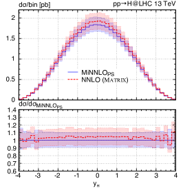
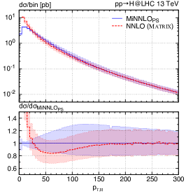
Figure 1: Comparison of NNLO (red) and MiNNLO_PS (blue) result for Higgs production via gluon fusion. The panel on the left (right) displays the Higgs boson rapidity (transverse momentum).

The agreement between the NNLO and the NNLO+PS prediction for the Higgs rapidity is very good, differences are of the order of few percent, the shape is predicted correctly and the size of the theoretical uncertainty also agrees rather well between the two predictions. For the Higgs transverse momentum, we observe good agreement at large $p_{\scriptscriptstyle\rm T,H}$ values, as expected by the fact that the MiNNLO_PS scale choice adopted in Ref. [7] is such that, at large $p_{\scriptscriptstyle\rm T,H}$, it approaches $M_{H}$, that is the scale used in the NNLO result. At low values of $p_{\scriptscriptstyle\rm T,H}$, the typical Sudakov shape is observed.

In Fig. 2 we show instead the rapidity of the dilepton system in Drell-Yan production (left) and the transverse momentum of the positron (right).

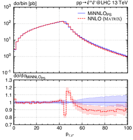
Figure 2: Comparison of NNLO (red) and MiNNLO_PS (blue) result for Drell-Yan production. The panel on the left (right) displays the dilepton rapidity (positron transverse momentum).

The agreement of the results for the $Z$-boson rapidity is very remarkable, and it also depends on the choice of the recoil scheme adopted in Pythia 8. The plot of the lepton transverse momentum shows the expected features: an extremely precise prediction below the Jacobian peak (with both results being NNLO accurate), a perturbative instability of the NNLO result close to the Jacobian peak that gets smooth by the PS, and a NLO-like uncertainty band of the two results above the peak, with a different normalization due to the different scale choices: for the NNLO result we have $\mu=M_{\ell\ell}$, whereas in MiNNLO_PS one has $\mu\simeq p_{\scriptscriptstyle\rm T,\ell\ell}$, and the region $p_{\scriptscriptstyle\rm T,\ell^{+}}\gtrsim M_{Z}/2$ is dominated by kinematic configurations where the $Z$ boson has a small transverse momentum.

As mentioned in the introduction, results for $Z\gamma$ [15] and $W^{+}W^{-}$ [16] production have been obtained recently with the MiNNLO_PS approach too, as well as NNLO+PS predictions for $t\bar{t}$ production [8]

References

References

- [1] K. Hamilton, P. Nason, C. Oleari and G. Zanderighi, JHEP 1305, 082 (2013) [arXiv:1212.4504].
- [2] K. Hamilton, P. Nason, E. Re and G. Zanderighi, JHEP 1310, 222 (2013) [arXiv:1309.0017 [hep-ph]].
- [3] S. Alioli, C. W. Bauer, C. J. Berggren, A. Hornig, F. J. Tackmann, C. K. Vermilion, J. R. Walsh and S. Zuberi, JHEP 09 (2013), 120 [arXiv:1211.7049 [hep-ph]].
- [4] S. Alioli, C. W. Bauer, C. Berggren, F. J. Tackmann, J. R. Walsh and S. Zuberi, JHEP 06 (2014), 089 [arXiv:1311.0286 [hep-ph]].
- [5] S. Höche, Y. Li and S. Prestel, Phys. Rev. D 91 (2015) no.7, 074015 [arXiv:1405.3607 [hep-ph]].
- [6] P. F. Monni, P. Nason, E. Re, M. Wiesemann and G. Zanderighi, JHEP 05 (2020), 143 [arXiv:1908.06987 [hep-ph]].
- [7] P. F. Monni, E. Re and M. Wiesemann, Eur. Phys. J. C 80 (2020) no.11, 1075 [arXiv:2006.04133 [hep-ph]].
- [8] J. Mazzitelli, P. F. Monni, P. Nason, E. Re, M. Wiesemann and G. Zanderighi, [arXiv:2012.14267 [hep-ph]].
- [9] M. Wiesemann, talk at Moriond 2021.
- [10] A. Karlberg, E. Re and G. Zanderighi, JHEP 09 (2014), 134 doi:10.1007/JHEP09(2014)134
- [11] W. Astill, W. Bizon, E. Re and G. Zanderighi, JHEP 06 (2016), 154 [arXiv:1603.01620 [hep-ph]].
- [12] W. Astill, W. Bizoń, E. Re and G. Zanderighi, JHEP 11 (2018), 157 [arXiv:1804.08141 [hep-ph]].
- [13] E. Re, M. Wiesemann and G. Zanderighi, JHEP 12 (2018), 121 [arXiv:1805.09857 [hep-ph]].
- [14] W. Bizoń, E. Re and G. Zanderighi, JHEP 06 (2020), 006 [arXiv:1912.09982 [hep-ph]].
- [15] D. Lombardi, M. Wiesemann and G. Zanderighi, [arXiv:2010.10478 [hep-ph]].
- [16] D. Lombardi, M. Wiesemann and G. Zanderighi, [arXiv:2103.12077 [hep-ph]].
- [17] S. Höche, Y. Li and S. Prestel, Phys. Rev. D 90 (2014) no.5, 054011 [arXiv:1407.3773 [hep-ph]].
- [18] S. Höche, S. Kuttimalai and Y. Li, Phys. Rev. D 98 (2018) no.11, 114013 [arXiv:1809.04192 [hep-ph]].
- [19] S. Alioli, C. W. Bauer, C. Berggren, F. J. Tackmann and J. R. Walsh, Phys. Rev. D 92 (2015) no.9, 094020 [arXiv:1508.01475 [hep-ph]].
- [20] S. Alioli, A. Broggio, S. Kallweit, M. A. Lim and L. Rottoli, Phys. Rev. D 100 (2019) no.9, 096016 [arXiv:1909.02026 [hep-ph]].
- [21] S. Alioli, A. Broggio, A. Gavardi, S. Kallweit, M. A. Lim, R. Nagar, D. Napoletano and L. Rottoli, JHEP 04 (2021), 254 [arXiv:2009.13533 [hep-ph]].
- [22] S. Alioli, A. Broggio, A. Gavardi, S. Kallweit, M. A. Lim, R. Nagar, D. Napoletano and L. Rottoli, JHEP 04 (2021), 041 [arXiv:2010.10498 [hep-ph]].
- [23] S. Alioli, A. Broggio, A. Gavardi, S. Kallweit, M. A. Lim, R. Nagar, D. Napoletanog, C. W. Bauer and L. Rottoli, [arXiv:2102.08390 [hep-ph]].
- [24] S. Alioli, A. Broggio, A. Gavardi, S. Kallweit, M. A. Lim, R. Nagar and D. Napoletano, Phys. Lett. B 818 (2021), 136380 [arXiv:2103.01214 [hep-ph]].
- [25] T. Cridge, M. A. Lim and R. Nagar, [arXiv:2105.13214 [hep-ph]].
- [26] Y. Hu, C. Sun, X. M. Shen and J. Gao, [arXiv:2101.08916 [hep-ph]].
- [27] R. Frederix and K. Hamilton, JHEP 05 (2016), 042 [arXiv:1512.02663 [hep-ph]].
- [28] S. Prestel, [arXiv:2106.03206 [hep-ph]].
- [29] P. F. Monni, E. Re and P. Torrielli, Phys. Rev. Lett. 116 (2016) no.24, 242001 [arXiv:1604.02191 [hep-ph]].
- [30] W. Bizon, P. F. Monni, E. Re, L. Rottoli and P. Torrielli, JHEP 02 (2018), 108 [arXiv:1705.09127 [hep-ph]].
- [31] M. Grazzini, S. Kallweit and M. Wiesemann, Eur. Phys. J. C 78 (2018) no.7, 537 [arXiv:1711.06631 [hep-ph]].