Fast and Slow Enigmas and Parental Guidance

Abstract

We describe several additions to the ENIGMA system that guides clause selection in the E automated theorem prover. First, we significantly speed up its neural guidance by adding server-based GPU evaluation. The second addition is motivated by fast weight-based rejection filters that are currently used in systems like E and Prover9. Such systems can be made more intelligent by instead training fast versions of ENIGMA that implement more intelligent pre-filtering. This results in combinations of trainable fast and slow thinking that improves over both the fast-only and slow-only methods. The third addition is based on ”judging the children by their parents”, i.e., possibly rejecting an inference before it produces a clause. This is motivated by standard evolutionary mechanisms, where there is always a cost to producing all possible offsprings in the current population. This saves time by not evaluating all clauses by more expensive methods and provides a complementary view of the generated clauses. The methods are evaluated on a large benchmark coming from the Mizar Mathematical Library, showing good improvements over the state of the art.

1 Introduction: The Fast and The Smart

Throughout the history of automated theorem proving, there have been two very different approaches to strengthening automated theorem provers (ATPs). The first one (the fast) relies on better engineering, such as improving the indexing for inference and reduction rules and on optimized low-level implementations. The gains achieved in this way can be quite high [31, 22, 38, 9, 28, 15].

The second approach (the smart) relies on advanced strategies and heuristics for guiding the proof search. This includes methods using extensive previous knowledge, e.g., various kinds of symbolic machine learning, such as the hints method in Otter [37] and Prover9 [19], and its watchlist [26] and proofwatch [6] variants implemented in E [29, 30]. With the recent advent of statistical machine learning (ML), a number of knowledge-based ATP-guiding methods have been created [11, 17, 3, 10]. This is done by compiling (extracting, compressing, generalizing) the previous knowledge into statistical ML predictors (models) that are then used to predict the usefulness of inference steps in the proof search.

The smart approaches, while potentially sophisticated and AI-motivated, may incur prohibitively high costs in their prediction modules, in particular when naively implemented [36, 21]. This can make them inferior in practice to faster alternative approaches, such as various kinds of randomization [25] and building of portfolios of complementary fast strategies [35, 27, 13]. This issue is getting increasingly important as deep learning (DL) is used for ATP guidance, sometimes with large cloud-based DL-predictors running on specialized hardware that hides the amount of resources used. It also complicates rigorous comparisons in established ATP competitions such as CASC/LTB [32, 33].

Another issue related to the use of expensive predictors can be summarized as the explore-exploit tradeoff introduced in reinforcement learning research [5]. In short, running an ATP guided by a 100-times slower predictor that is only slightly better (possibly due to insufficient previous data for learning) will not only typically solve fewer problems due to much more expensive backtracking but also generate much less data for training the predictor in the next iteration. Hence, given a global time limit allowing many proving/learning iterations over a large set of related problems in a realistic problem-solving setup such as CASC LTB, a faster predictor will in the same time generate much more data to learn from. This in turn often leads to better performance: a slightly weaker ML system trained on much more data will often ultimately outperform a slightly stronger ML system trained on much less data.

1.1 Contributions

In this work we develop combinations of the fast(er) and smart(er) approaches in the context of the learning-guided ENIGMA framework. After giving a summary of ENIGMA in Section 2, Section 3 introduces our new methods.

First, Section 3.1 describes a large increase in the speed of neural guidance in ENIGMA. We add an efficient server-based evaluation that uses dedicated GPUs instead of a CPU. When using four commodity GPU cards, this speeds up the neural evaluation of the clauses about four times in real time.

Section 3.2 describes the second addition, motivated by fast weight-based rejection filters used in systems such as E and Prover9. Such methods can be replaced by training fast predictors that implement more intelligent pre-filtering. In the context of ENIGMA, fast(er) is easy to implement by variously parameterized predictors based on gradient-boosted decision trees (GBDTs). Slow(er) models are in those based on graph neural networks (GNNs).

Section 3.3 describes the third addition based on ”judging the children by their parents”, i.e., possibly rejecting an inference before it even produces a clause. This grants the machine learning methods greater control of the proof search and saves time by not evaluating all clauses by more expensive methods, also providing a complementary view of the generated clauses.

In Section 4 we describe the experimental setting and a large evaluation corpus based on the Mizar Mathematical Library and its MPTP translation. We also present our baseline methods there. Section 5 evaluates the new methods and shows that even in relatively low time limits the methods provide good performance improvements over the previous versions of ENIGMA.

2 Saturation Proving and Its Guidance by ENIGMA

State-of-the-art automated theorem provers (ATP), such as E, Prover9, and Vampire [20], are based on the saturation loop paradigm and the given clause algorithm [24]. The input problem, in first-order logic (FOF), is translated into a refutationally equivalent set of clauses, and a search for contradiction is initiated. The ATP maintains two sets of clauses: processed (initially empty) and unprocessed (initially the input clauses). At each iteration, one unprocessed clause is selected (given), and all of the possible inferences with all the processed clauses are generated (typically using resolution, paramodulation, etc.), extending the unprocessed clause set. The selected clause is then moved to the processed clause set. Hence the invariant holds that all the mutual inferences among the processed clauses have been computed.

The selection of the “right” given clause is known to be vital for the success of the proof search. The ENIGMA system [11, 12, 14, 7, 3, 10] applies various machine learning methods for given clause selection, learning from a large number of previous successful proof searches. The training data consists of clauses processed during a proof search, labeling the clauses that appear in the discovered proof as positive, and the other (thus unnecessary) processed clauses as negative.

The first ENIGMA [11] used fast linear classification [4] with hand-crafted clause features based on symbol names, representing clauses by fixed-length numeric vectors. Follow-up versions [12, 14, 7, 3] introduced context-based clause evaluation and fast dimensionality reduction by feature hashing, and employed Gradient Boosting Decision Trees (GBDTs), implemented by the XGBoost and LightGBM systems [2, 18]), and Recursive Neural Networks (implemented in PyTorch) as the underlying machine learning methods.

The latest version, ENIGMA Anonymous [10], abstracts from name-based clause representations and provides the best results so far both with GBDTs and Graph Neural Networks (GNNs) [1]. For GBDTs, clauses are again represented by fixed-length vectors based on syntax trees and anonymization is achieved by replacing symbol names by their arities. Our GNN [23] represents clauses by variable-length numeric tensors encapsulating syntax trees as graph structures with symbol names omitted. ENIGMA-GNN evaluates new clauses jointly in larger batches (queries) and with respect to a large number of already selected clauses (context). The GNN predicts the collectively most useful subset of the clauses in several rounds (layers) of message passing. This means that approximative inference rounds done by the GNN are efficiently interleaved with precise symbolic inference rounds done inside E. The GBDT and GNN versions have so far been used separately and only with CPU-based evaluation. In this work, we add efficiently implemented GPU-based evaluation for the GNN and start to use the two methods cooperatively.

3 Cooperative Filtering: Faster and Smarter

The set of generated clauses in saturation-style ATPs typically grows quadratically with the number of processed clauses. Each new given clause is combined with all compatible previously processed clauses, followed by (possibly expensive) evaluation of all newly generated clauses. In particular, the GNN predictors typically incur a significant evaluation cost per clause. The quadratic growth means that longer ENIGMA-GNN runs may get very slow.

To avoid large memory consumption and similar expensive evaluations in long hint-based Prover9 runs (often taking several days) on the AIM problems [19], Veroff has used weight-based filtering, discarding immediately clauses that reach a certain weight limit. This often helps, but counterexamples are common, and in practice, such schemes often need to be made more complicated. The three methods that we introduce below are instead targeting this issue by using faster learning-based filtering.

3.1 Fast GNN Evaluation Using a GPU Server

The main weakness of the GNN version of ENIGMA is its slow clause evaluation. In our previous ENIGMA Anonymous experiments[10], we used GPUs for model training, but during the proof search we evaluated the clauses on a single CPU (per each E prover’s instance). This was partly to provide a fair comparison with GBDTs which we also evaluate on a single CPU, but also to avoid large start-up overheads when loading the neural models to a GPU and running with low time limits. Here we instead develop a persistent multi-threaded GPU server that evaluates clauses from multiple E prover runs using multiple GPUs.

The modification is as follows. During the proof search, after computing the tensor representation of the newly generated clauses, an E Prover client sends the tensors (in a JSON text format) over a network socket to a remote server. The client then waits for the server response which provides the scores (GNN evaluations) of the new clauses. This means that the clients are inactive for some time and more of them are needed to saturate the CPUs on the machines (see the detailed experimental discussion in Section 5.1). This is typically not a problem due to many instances of E running with different premises and parameters in hammering and CASC LTB scenarios, as well as in many iterations of the learning/proving loop that attempt to solve harder and harder problems over a large problem set.

The remote server, written in Python, is launched before the E clients, loading the GNN model to the (multiple) GPUs in advance. Once the model is loaded to the GPUs, the server accepts tensor queries on a designated port, evaluates them on the GPUs, and sends the clause evaluations back to the clients. In more detail, the server is parameterized by the number $N$ (our default is 28) of independent worker threads, the batch size $b$ (our default is 8) and the waiting time $T$ (our default is 0.01s). The client queries are accumulated in a shared queue that the $N$ worker threads process. Each worker operates in two steps. First, it checks the queue, and if it contains less than $b$ queries, it waits for $T$ seconds. Then it evaluates the first $b$ queries on the queue, or less if there are not enough of them available. Note that when the worker waits or evaluates queries, other workers can process the queue.

The advantage is that the single GNN server amortizes the startup costs and handles queries of many E prover clients and distributes them across multiple GPUs. This means that much larger batches (containing clauses coming from multiple clients) are typically loaded onto the GPUs, amortizing also the relatively high cost of communication with the GPUs. This results in large real time speed-ups over the CPU version, see Section 5.1. In our experiments, we run the GPU server and the E clients on the same machine. Hence the network overhead is low because the communication is done over a local loopback interface. In the case of a remote connection, the architecture would benefit from data compression and/or binary data formats to decrease the network overhead. See Section 5.1 for the current average sizes of the data exchanged.

3.2 Best of Both Worlds: GNN with GBDT Filtering

While the GPU server evaluation provides a considerable speed up, the evaluation of clauses on a GPU is still relatively costly compared to the GBDT clause evaluation. Hence we develop the following combination of the two methods, where the GBDT is used to pre-filter the clauses for the GNN.

In more detail, the set of clauses to be evaluated by the GNN is first evaluated by a fast GBDT model. The GBDT model assigns a score between $0$ and $1$ to each clause, and only the clauses with scores higher than a selected threshold are sent to the GPU server for evaluation by the GNN. The clauses which are filtered out by the GBDT model are assigned a very high weight inside E Prover, which makes them unlikely to ever be selected for processing. This way we prevent E from incorrectly reporting satisfiability when the good clauses run out.

Several requirements must be met for this filtering to be effective. First, the GBDT filtering model must be small enough so that the evaluation is fast, yet precise enough so that the more important clauses are not mistakenly filtered out too often. Second, the score threshold must be properly fine-tuned, which typically requires experimental grid search on smaller samples. Experiments with a GBDT pre-filtering for a GNN are presented in Section 5.2.

3.3 Parental Guidance: Pruning the Given Clause Loop

We define (clausal) parental guidance as clause evaluation based on the features of the parents of a clause rather than on the clause itself. Such fast rejection filters often help: in nature, mating is typically highly restricted by various features of parents (e.g., their age, appearance, finances, etc.). Similarly, it does not often happen that clauses from very different parts of mathematics (e.g., differential geometry and graph theory) need to be resolved.

Parental guidance can be seen as “just another filter” of the generated clauses, but its motivation is more radical: The “good old” given clause loop [24] insists, for completeness reasons, on performing all possible inferences between the processed clauses and the given clause, typically leading to a quadratic growth of the set of generated clauses. However, if we had perfect information about the proof, this would be wasteful and could be replaced by just performing the inferences needed for the proof in each given clause loop. With parental guidance, we instead propose to prune the given clause loop in a soft way: a trained predictor judges the likelihood of the particular inference being needed for the proof. When an inference is deemed useless, the clause is still generated but immediately frozen so that it does not have to be evaluated by additional heuristics.

The parental guidance is implemented using GBDTs (our parental model), and the filter is directly put inside E’s given clause loop as follows. When E selects a given clause $g$, E uses term indexes to efficiently determine which clauses can be combined with $g$ to generate new clauses. After generating the clauses, E performs simplifications, removes trivial clauses, evaluates the remaining clauses with the clause evaluation functions, and inserts them into the unprocessed set. The call to the parental model is executed after the clause generation and prior to the simplifications. Clauses generated by paramodulation, which also implements resolution in E, have two parents, and these are judged by the parental model. Clauses whose parents are jointly scored below a chosen threshold are put into the freezer set to avoid impairing the completeness of the proof search. Clauses with good parents continue on to the unprocessed set. In case the unprocessed set becomes empty, the frozen clauses are revived and treated as usual.

Note that a naive alternative way to implement parental guidance would be to evaluate each given clause’s compatibility with all previously processed clauses. This would, however, result in many unnecessary GBDT queries and evaluations. Instead, our approach allows E’s indexing to find the typically much smaller set of potential inferences and to limit the parental evaluation to them.

There are various ways to represent the pair of parent clauses for the learning of the parental model. In this work, we evaluate two methods:

1. $\mathcal{P}_{\textsf{fuse}}$ merges the feature vectors of the parent clauses into one vector, typically by simply adding the feature counts

2. $\mathcal{P}_{\textsf{cat}}$ concatenates the feature vectors of the parent clauses to preserve their information in full.

An interesting future alternative is to include the difference of the parents’ feature vectors in addition to their union and concatenation, which allows the GBDT to choose the most informative features.

4 Experimental Setting and Baselines

4.1 Evaluation Problems and Training Data

All our experiments are performed on a large benchmark of $57\,880$ problems originating from the Mizar Mathematical Library (MML) [16] exported to first-order logic by MPTP [34]. We make use of our ongoing extensive evaluation of many AI/TP methods over this corpus that measures the overall improvement on this large dataset over the last similar evaluation done in [16]. In these experiments we have significantly extended our previously published results [10]. Proofs of 73.5% (more than $40$k) Mizar problems have been so far found by learning-guided ATPs, and numerous GBDT and GNN models for ATP guidance have been trained.

In that experiment, all Mizar problems are split (in a 90-5-5% ratio) into $3$ subsets: (1) $52$k problems for training, (2) $2896$ problems for development, and (3) $2896$ problems for final evaluation (holdout). We use this split here, and additionally we use a random subset of $5792$ of the training problems to speed up the training of various experimental methods.

4.2 Baseline ENIGMA Models

Out of the $52$k training problems, we were previously able to prove more than $36$k problems, obtaining varied numbers of proofs for each problem (ranging from $1$ to hundreds). On these $36$k problems we train our baseline GBDT and GNN predictors. To balance the contribution of different problems during the training of the predictors, we randomly choose at most 3 proofs for every proved training problem. This yields a set of about $100$k proofs, denoted further as the large (training) set. When limited to the $5792$ random subset of the training problems, this yields $11\,748$ proofs, denoted further as the small training set.

On the large set we train the first baseline predictor denoted by $\mathcal{D}_{\textsf{large}}$. This is a GBDT model (implemented by the LightGBM framework) trained using the ENIGMA Anonymous clause representation (Section 2). The model consists of $150$ decision trees of depth $40$ with $2048$ leaves. This model was selected as it performed best in our previous experiments with standard GBDTs, being able to prove $1377$ of the holdout problems using a 5 second limit per problem. Additionally, we train another model $\mathcal{D}_{\textsf{small}}$ only on the small set of training problems. The model $\mathcal{D}_{\textsf{small}}$ is a LightGBM model with $150$ trees of depth $30$ and with $9728$ leaves. The training of $\mathcal{D}_{\textsf{large}}$ took around $27$ minutes and the training of $\mathcal{D}_{\textsf{small}}$ around $10$ minutes, both on $30$ CPUs. These are relatively low and practical times compared to the training of neural networks.

We also train baseline GNN models on the same data, denoted $\mathcal{G}_{\textsf{large}}$ and $\mathcal{G}_{\textsf{small}}$ respectively. The training of $\mathcal{G}_{\textsf{large}}$ for 45 epochs takes about 15 hours on the full set of 100k proofs on a high-end NVIDIA V100 GPU card. It would likely take days when training with CPUs only. We choose for the ATP evaluation the (39th) snapshot that achieves both the best loss (0.2063) and the best weighted accuracy (0.9147) on 5% of the data that we do not use for training. The training of $\mathcal{G}_{\textsf{small}}$ for 100 epochs takes about 4 hours on the small set using the same GPU card. We choose for the ATP evaluation the (56th) snapshot that achieves the best loss (0.2988) on 5% of the data that we do not use for training. The weighted accuracy on this set is 0.8685, which is also among the highest values.

In the evaluation we run all our baseline ENIGMA predictors in an equal combination with a strong non-learning E strategy $\mathcal{S}$ (see Appendix 0.A). This means that the processed clauses are selected in (equal) turns by ENIGMA and by $\mathcal{S}$. This coop mode has typically worked better than the solo mode, where only the ENIGMA predictor is doing the clause selection.

4.3 Training of the Parental GBDT Models

The training data for the parental guidance models are generated by running E using either $\mathcal{D}_{\textsf{large}}$ or $\mathcal{G}_{\textsf{large}}$ on the $52$k training problems with a 30 second time limit and by printing the derivation of all clauses generated during the proof search. We considered the following two schemes to classify the good pairs of parents and to generate the training data:

1. $\mathcal{P}^{\textsf{proof}}$ classifies parents of only the proof clauses as positive and all other generated clauses as negative.

2. $\mathcal{P}^{\textsf{given}}$ classifies parents of all processed (selected) clauses as positive and the unprocessed generated clauses as negative.

The rationale behind $\mathcal{P}^{\textsf{proof}}$ is that every non-proof clause should be pruned if possible. The rationale behind $\mathcal{P}^{\textsf{given}}$ is that if an effective clause selection strategy, such as $\mathcal{D}_{\textsf{large}}$, predicted a clause to be useful, then it is probably worth generating. However, such data may be confusing as it includes clauses that did not contribute to the proof.

If a pair of parents produces both positive and negative clauses, we consider the pair positive in our implementation. However, this does not happen very often. Based on a survey on the small set labeled according to $\mathcal{P}_{\textsf{fuse}}^{\textsf{proof}}$, 73% of the problems have no conflict. There are $1519$ parents of both positive and negative clauses, $53\,359$ are positive, and $6\,086\,414$ are negative. Under $\mathcal{P}_{\textsf{fuse}}^{\textsf{given}}$, $9798$ of the parents are mixed, $854\,778$ are positive, and $5\,178\,592$ are negative. In either case, the primary learning task is to identify and prune as many negative clauses as possible without filtering a necessary proof clause by mistake.

One parameter to experimentally tune is the pos-neg ratio used in the GBDT training: the ratio of positive and negative examples. The pos-neg ratio is $1$:$192$ over the large $\mathcal{P}_{\textsf{fuse}}^{\textsf{proof}}$ data, which is more than ten times more than the ratio of the training data for $\mathcal{D}_{\textsf{large}}$ and $\mathcal{G}_{\textsf{large}}$. Hence, reducing the pos-neg ratio by randomly sampling negative examples could further boost the training performance.

The parental guidance models are trained using GBDTs. Trained models are evaluated in combination with the GBDT or GNN clause evaluation heuristic using either the $\mathcal{D}_{\textsf{large}}$ or $\mathcal{G}_{\textsf{large}}$ model, see Section 5.3.

5 Evaluation of the New Methods

5.1 Speedup by Using a GPU Server

First we measure the speedup obtained by evaluating the ENIGMA GNN calls on a separate GPU server. To avoid network latency and for a cleaner comparison, we run both the clients (E/ENIGMA) and the GPU server on the same machine equipped with four NVIDIA GeForce GTX 1080 GPU cards and 36 hyperthreading CPU cores. We configure the server to use all four GPU cards. Its other important parameters are the number of worker threads and the batch size. We experimentally set them to 28 and 8, and we use $\mathcal{G}_{\textsf{large}}$ for all proof runs.

Comparison of the CPU-only and GPU-server versions is complicated by the fact that the server-based GNN evaluations do not count towards the CPU time taken by E, as reported by the operating system. Still, a comparison using the CPU time is interesting and we include it, using 30 and 60 second CPU limits for the CPU-only version, and a 30 second CPU limit for the client-server version.

Another way to compare the two is by using parallelization, i.e., running many instances of E in parallel. In the client-server version the instances talk to the GPU server simultaneously. We saturate the machine’s CPUs fully for both versions, and run for approximately equal overall real time over the development and holdout sets. This is roughly achieved by using 60s time limit with 70-fold parallelization for the CPU version, and 30s time limit with 160-fold parallelization for the client/server version. The CPU version then takes about $27.5$ minutes to finish on the $2896$ problems, while the client-server takes about 34 minutes to finish. Table 1 compares the number of solved problems on the development and holdout sets. The GPU server improves the performance on the development resp. holdout sets by 9.5% resp. 11.5%.

We also compare the average number of generated clauses on the problems that timed out in both versions. In the 60s CPU version it is $16\,835$, while in the 30s client-server it is $63\,305$. This is a considerable speedup, achieved by employing the additional custom hardware—our four GPU cards. The average number of GNN queries in the 1358 problems that timed out in the 30s GPU server runs is 243.8, and on average the communication with the GPU server took 155MB in a timed-out problem. A single GNN query took on average 637kB.

Table 1: Comparison of the CPU-only GNN ENIGMA with the client-server version using GPUs. All runs are evaluating $\mathcal{G}_{\textsf{large}}$ on the whole development (D) and holdout (H) datasets. The percentage improvement is computed over the 60s CPU version that corresponds more closely in real time to the client-server version. All runs use queries of size 256 and contexts of size 768.

set	model	method	time	solved
D	$\mathcal{G}_{\textsf{large}}$	CPU	30	1311
D	$\mathcal{G}_{\textsf{large}}$	CPU	60	1380
D	$\mathcal{G}_{\textsf{large}}$	GPU	30	1511 (+9.5%)

set	model	method	time	solved
H	$\mathcal{G}_{\textsf{large}}$	CPU	30	1301
H	$\mathcal{G}_{\textsf{large}}$	CPU	60	1371
H	$\mathcal{G}_{\textsf{large}}$	GPU	30	1529 (+11.5%)

5.2 Evaluation of 2-phase ENIGMA

5.2.1 Small GBDT and Small GNN:

In the first experiment we use the GBDT and GNN predictors $\mathcal{D}_{\textsf{small}}$ and $\mathcal{G}_{\textsf{small}}$ trained on the small subset of the training dataset.

We first do a grid search over the parameters on a smaller dataset of 300 development problems (see Table 9 in Appendix 0.B for the full grid search). Then we evaluate the best parameters on the development and holdout sets and compare them with the standalone performance of $\mathcal{G}_{\textsf{small}}$, which is the stronger of the two baselines (Table 2). The best combined methods are then evaluated also in 60s. This gives a relatively fair real-time comparison to the standalone GNN, because the reported CPU times do not include the time taken by the GPU server.

Our best combined method solves (in real time) 10.4%, resp. 9.0%, more problems on the development, resp. holdout, set than the standalone GNN. This is a significant improvement, which will likely get even more visible with higher time limits, because of the quadratic growth of the set of generated clauses. The performance improvement over the standalone GBDT model is even larger.

Table 2: Final evaluation of the best combination of $\mathcal{D}_{\textsf{small}}$ with $\mathcal{G}_{\textsf{small}}$ on the whole development (D) and holdout (H) datasets.

set	model	thresh.	time	query	context	solved
D	$\mathcal{G}_{\textsf{small}}$	-	30	256	768	1251
D	$\mathcal{D}_{\textsf{small}}$	-	30	-	-	1011
D	$\mathcal{D}_{\textsf{small}}$+$\mathcal{G}_{\textsf{small}}$	0.01	60	512	1024	1381 (+10.4%)
D	$\mathcal{D}_{\textsf{small}}$+$\mathcal{G}_{\textsf{small}}$	0.03	60	512	1024	1371 (+9.6%)
D	$\mathcal{D}_{\textsf{small}}$+$\mathcal{G}_{\textsf{small}}$	0.03	30	512	1024	1341 (+7.2%)
D	$\mathcal{D}_{\textsf{small}}$+$\mathcal{G}_{\textsf{small}}$	0.01	30	512	1024	1339 (+7.0%)
H	$\mathcal{G}_{\textsf{small}}$	-	30	256	768	1277
H	$\mathcal{D}_{\textsf{small}}$	-	30	-	-	1002
H	$\mathcal{D}_{\textsf{small}}$+$\mathcal{G}_{\textsf{small}}$	0.01	60	512	1024	1392 (+9.0%)
H	$\mathcal{D}_{\textsf{small}}$+$\mathcal{G}_{\textsf{small}}$	0.03	60	512	1024	1387 (+8.6%)
H	$\mathcal{D}_{\textsf{small}}$+$\mathcal{G}_{\textsf{small}}$	0.01	30	512	1024	1361 (+6.6%)
H	$\mathcal{D}_{\textsf{small}}$+$\mathcal{G}_{\textsf{small}}$	0.03	30	512	1024	1353 (+6.0%)

5.2.2 Large GBDT and Small GNN:

In the next experiment, we want to see how much the training of the less expensive model (GBDT) on more data helps. I.e., we replace $\mathcal{D}_{\textsf{small}}$ with $\mathcal{D}_{\textsf{large}}$ and keep $\mathcal{G}_{\textsf{small}}$. This has practical applications in real time, because cheaper ML predictors such as GBDTs are faster to train than more expensive ones such as the GNN. We again first do a grid search over the parameters on a small dataset of 300 development problems (see Table 10 in Appendix 0.B). Then we evaluate the best models on the development and holdout sets and compare them with the standalone performance of $\mathcal{D}_{\textsf{large}}$ and $\mathcal{G}_{\textsf{small}}$ (Table 3). The best combined methods are then again evaluated also in 60s, which makes it comparable in real time to the standalone GNN model.

Table 3: Final evaluation of the best combination of $\mathcal{D}_{\textsf{large}}$ and $\mathcal{G}_{\textsf{small}}$ on the whole development (D) and holdout (H) datasets.

set	model	thresh.	time	query	context	solved
D	$\mathcal{G}_{\textsf{small}}$	-	30	256	768	1251
D	$\mathcal{D}_{\textsf{large}}$	-	30	-	-	1397
D	$\mathcal{D}_{\textsf{large}}$+$\mathcal{G}_{\textsf{small}}$	0.3	60	2048	768	1527 (+9.3%)
D	$\mathcal{D}_{\textsf{large}}$+$\mathcal{G}_{\textsf{small}}$	0.3	30	2048	768	1496 (+7.1%)
H	$\mathcal{G}_{\textsf{small}}$	-	30	256	768	1277
H	$\mathcal{D}_{\textsf{large}}$	-	30	-	-	1390
H	$\mathcal{D}_{\textsf{large}}$+$\mathcal{G}_{\textsf{small}}$	0.3	60	2048	768	1494 (+7.5%)
H	$\mathcal{D}_{\textsf{large}}$+$\mathcal{G}_{\textsf{small}}$	0.3	30	2048	768	1467 (+5.5%)

Our best combined method solves (in CPU time) 7.1%, resp. 5.5%, more problems on the development, resp. holdout, set than the standalone GBDT. For the GNN, this is (in real time) 9.3% resp. 7.5%. These are smaller gains than in the previous $\mathcal{D}_{\textsf{small}}+\mathcal{G}_{\textsf{small}}$ scenario, most likely because the stronger predictor dominates here. Also note that the large query ($2048$) used in our strongest model is typically diminished a lot by the GBDT pre-filter, resulting in average query sizes after the GBDT pre-filtering of 256–512.

5.2.3 Large GBDT and Large GNN:

Finally, we evaluate the large setting, using the GBDT and GNN predictors $\mathcal{D}_{\textsf{large}}$ and $\mathcal{G}_{\textsf{large}}$ trained on the full training dataset. Again, we first do a grid search over the parameters on the small set of 300 development problems (Table 11 in Appendix 0.B). Then we evaluate the best parameters on the development and holdout sets, and we compare them with the standalone performance of $\mathcal{D}_{\textsf{large}}$ and $\mathcal{G}_{\textsf{large}}$ (Table 4). The improvements on the development, resp. holdout, set is 9.1%, resp. 7.3%, in real time, and 6.9%, resp. 4.8%, when using CPU time. The E auto-schedule solves in 30s (CPU time) 1020 of the holdout problems. Our strongest 2-phase method solves 1602 of these problems in the same CPU time, i.e., 57.1% more problems.

Table 4: Final evaluation of the best combination of $\mathcal{D}_{\textsf{large}}$ and $\mathcal{G}_{\textsf{large}}$ on the whole development (D) and holdout (H) datasets.

set	model	thresh.	time	query	context	solved
D	$\mathcal{G}_{\textsf{large}}$	-	30	256	768	1511
D	$\mathcal{D}_{\textsf{large}}$	-	30	-	-	1397
D	$\mathcal{D}_{\textsf{large}}$+$\mathcal{G}_{\textsf{large}}$	0.1	60	1024	768	1648 (+9.1%)
D	$\mathcal{D}_{\textsf{large}}$+$\mathcal{G}_{\textsf{large}}$	0.1	30	1024	768	1615 (+6.9%)
H	$\mathcal{G}_{\textsf{large}}$	-	30	256	768	1529
H	$\mathcal{D}_{\textsf{large}}$	-	30	-	-	1390
H	$\mathcal{D}_{\textsf{large}}$+$\mathcal{G}_{\textsf{large}}$	0.1	60	1024	768	1640 (+7.3%)
H	$\mathcal{D}_{\textsf{large}}$+$\mathcal{G}_{\textsf{large}}$	0.1	30	1024	768	1602 (+4.8%)

5.3 Evaluation of the Parental Guidance Combined with $\mathcal{D}_{\textsf{large}}$

The parameters for parental guidance models are explored via a series of grid searches to reduce the number of combinations. Initially, we only use $\mathcal{D}_{\textsf{large}}$ in conjunction with the parental models. First, the training data classification schemes, $\mathcal{P}_{\textsf{fuse}}^{\textsf{proof}}$ and $\mathcal{P}_{\textsf{fuse}}^{\textsf{given}}$, are compared with a grid search over the pos-neg reduction ratio. The best combination of reduction ratio and classification scheme is used to perform a grid search over LightGBM parameters for $\mathcal{P}_{\textsf{fuse}}$. Next, reduction ratio and LightGBM parameter grid searches are done with the $\mathcal{P}_{\textsf{cat}}$ featurization method data, starting with the best $\mathcal{P}_{\textsf{fuse}}$ parameters from the previous experiments. Every model is evaluated with the same set of nine parental filtering thresholds $\{0.005,0.01,0.03,0.05,0.1,0.2,0.3,0.4,0.5\}$. The grid searches are done over the $300$ problem development set and run for $30$ seconds. On this dataset, $\mathcal{D}_{\textsf{large}}$ solves 159 problems.

5.3.1 Pos-neg reduction ratio tuning (merge):

The first grid search examines the pos-neg reduction ratio denoted as $\rho$. Before the reduction, the average pos-neg ratio for $\mathcal{P}_{\textsf{fuse}}^{\textsf{given}}$ is $1:9.2$ and the average for $\mathcal{P}_{\textsf{fuse}}^{\textsf{proof}}$ is $1:191.8$. We reduce the pos-neg ratio to a given $\rho$ by randomly sampling the negative examples on a problem-specific basis. This means that the average pos-neg ratio over the whole dataset is typically a bit smaller than $\rho$. For example, using $\rho=4$ on the $\mathcal{P}_{\textsf{fuse}}^{\textsf{proof}}$ results in an average of $3.95$ times more negative than positive examples. Both $\mathcal{P}_{\textsf{fuse}}^{\textsf{given}}$ and $\mathcal{P}_{\textsf{fuse}}^{\textsf{proof}}$ are tested using $\rho\in\{-,1,2,4,8,16\}$ where “$-$” denotes using the full training dataset. We use the best LightGBM model parameters discovered during prototyping of the parental guidance features: the parameters are $50$ trees of depth $13$ with $1024$ leaves.

Table 5: The best threshold for each tested reduction ratio. The threshold of 0.03 was identical to 0.05 for all tested ratios with $\mathcal{P}_{\textsf{fuse}}^{\textsf{given}}$, whereas there are no ties among thresholds for $\mathcal{P}_{\textsf{fuse}}^{\textsf{proof}}$.

$\rho_{\textsf{fuse}}^{\textsf{given}}$	$-$	1	2	4	8	16
threshold	0.05	0.05	0.05	0.05	0.05	0.05
solved	161	161	161	161	161	160

$\rho_{\textsf{fuse}}^{\textsf{proof}}$	$-$	1	2	4	8	16
threshold	0.005	0.2	0.2	0.2	0.2	0.2
solved	111	164	163	165	162	164

Table 5 shows that the reduction ratio makes significant difference for the $\mathcal{P}_{\textsf{fuse}}^{\textsf{proof}}$ data and almost none for $\mathcal{P}_{\textsf{fuse}}^{\textsf{given}}$ data, which is probably because the $\mathcal{P}_{\textsf{fuse}}^{\textsf{given}}$ data are already reasonably balanced. Moreover, parental guidance seems to perform better with $\mathcal{P}_{\textsf{fuse}}^{\textsf{proof}}$ data than $\mathcal{P}_{\textsf{fuse}}^{\textsf{given}}$ data, probably because mistakes of $\mathcal{D}_{\textsf{large}}$ are included in the training data. In the following experiments, only the $\mathcal{P}^{\textsf{proof}}$ classification scheme is used (so the prefix is dropped).

5.3.2 LightGBM parameter tuning (merge):

Next we perform the second grid search over the LightGBM training hyper-parameters for $\mathcal{P}_{\textsf{fuse}}$, fixing $\rho=4$ as it performed best. We try the following values for the three main hyper-parameters, namely, for the number of trees in a model, the maximum number of tree leaves, and the maximum tree depth:

$$\mathrm{trees} \in \{50,100,150\}$$

$$\mathrm{leaves} \in \{1024,2048,4096,8192,16384\}$$

$$\mathrm{depth} \in \{13,40,60,256\}$$

The best model for $\mathcal{P}_{\textsf{fuse}}$ solves $171$ problems and consists of $100$ trees, with the depth $40$, and $8192$ leaves, and a threshold of $0.05$. Another eight models solve $169$ problems. We also tested these parameters to find a better model for $\mathcal{P}_{\textsf{fuse}}^{\textsf{given}}$, which solves $163$ problems with $\rho=8$ and a threshold of $0.1$.

Table 6: The best threshold for each tested reduction ratio of $\mathcal{P}_{\textsf{cat}}$.

$\rho_{\textsf{cat}}$	$-$	1	2	4	8	16
threshold	0.5	0.1	0.05	0.3	0.1	0.05
solved	117	168	170	168	173	169

5.3.3 Pos-neg reduction ratio tuning (concat):

This grid search uses the best LightGBM hyper-parameters for $\mathcal{P}_{\textsf{fuse}}$ to test the same reduction ratios and thresholds for $\mathcal{P}_{\textsf{cat}}$. Table 6 shows that $\mathcal{P}_{\textsf{cat}}$ outperforms $\mathcal{P}_{\textsf{fuse}}$ and $\rho=8$ is the best. Reducing the negatives is even more important here.

5.3.4 LightGBM parameter tuning (concat):

The grid search for the $\mathcal{P}_{\textsf{cat}}$ data is done over the following hyper-parameters:

$$\mathrm{trees} \in \{50,100,150,200\}$$

$$\mathrm{leaves} \in \{1024,2048,4096,8192,16384,32768\}$$

$$\mathrm{depth} \in \{13,40,60,256,512\}$$

The upper limits have increased compared to the $\mathcal{P}_{\textsf{fuse}}$ grid-search because one of the best models had $150$ trees of depth $256$, placing it at the edge of the grid. The best models solve $174$-$175$ problems. These are evaluated on the full development set (Table 7). The larger models seem to work best with a threshold of $0.05$ and the smaller models with a threshold of $0.2$, which is likely because they can be less precise. The full distribution of the results can be seen in Figure 1. The number of parameter configurations that outperform the baseline suggests that parental guidance is an effective method.

Table 7: The best $\mathcal{P}_{\textsf{cat}}$ models with $\rho=8$.

trees	depth	leaves	threshold	solved (300)	solved (D)
200	60	4096	0.05	175	1557
200	512	4096	0.05	175	1561
200	256	4096	0.05	174	1558
150	512	1024	0.2	174	1568
150	256	1024	0.2	174	1556
100	60	8192	0.05	174	1571
100	40	2048	0.2	174	1544
100	40	2048	0.1	174	1544

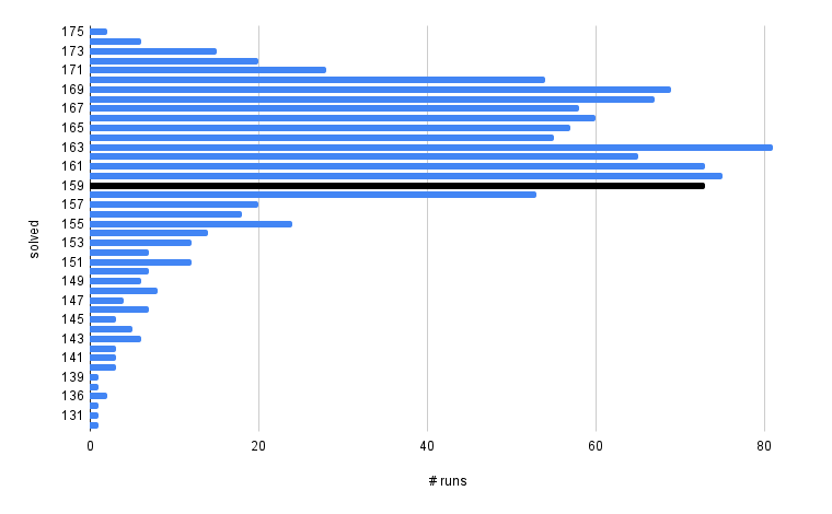
Figure 1: The number of settings (and runs) corresponding to each number of solutions for the $\mathcal{P}_{\textsf{cat}}$ grid search. The black bar is $159$, the number of problems solved by $\mathcal{D}_{\textsf{large}}$. Only $154$ (20%) of the runs interfere with $\mathcal{D}_{\textsf{large}}$’s performance and solve fewer problems. These runs largely consist of the thresholds, $\{0.3,0.4,0.5\}$, but the only parameter whose majority of runs score below $\mathcal{D}_{\textsf{large}}$ is a threshold of $0.5$. The outliers tend to be larger models.

Table 8: Final 30s evaluation on small trains (T), development (D), and holdout (H) compared with $\mathcal{D}_{\textsf{large}}$.

model	threshold	solved (T)	solved (D)	solved (H)
$\mathcal{D}_{\textsf{large}}$	-	3269	1397	1390
$\mathcal{P}_{\textsf{fuse}}^{\textsf{given}}$+$\mathcal{D}_{\textsf{large}}$	0.05	3302 (+1.0%)	1411 (+1.0%)	1417 (+1.9%)
$\mathcal{P}_{\textsf{fuse}}^{\textsf{proof}}$+$\mathcal{D}_{\textsf{large}}$	0.1	3389 (+3.7%)	1489 (+6.6%)	1486 (+6.9%)
$\mathcal{P}_{\textsf{cat}}$+$\mathcal{D}_{\textsf{large}}$	0.05	3452 (+5.6%)	1571 (+12.4%)	1553 (+11.7%)

Finally we evaluate the best models on the small training, development, and holdout sets, and we compare them with the standalone performance of $\mathcal{D}_{\textsf{large}}$ (Table 8). Parental guidance achieves a significant improvement in performance on all datasets, solving $11.7$% more on the holdout set. It is interesting to note that the improvement is greater on the development and holdout sets than on the training set. For parental guidance it seems superior to classify only proof clauses as positive examples. This is most likely due to LightGBM being confused by processed clauses that did not contribute to any proof. The method of concatenating the parent clause feature vectors ($\mathcal{P}_{\textsf{cat}}$) seems far superior to merging them ($\mathcal{P}_{\textsf{fuse}}$). This is likely because merging the features is lossy and the order of the parents matters when performing inferences.

The results indicate that pruning clauses prior to clause evaluation is helpful. ENIGMA models tend to run best in equal combination with a strong E strategy, but this means they have no control over 50% of the clauses selected for processing. The ability to filter which clauses the strong E strategy can evaluate and select may be part of the strength behind parental guidance.

5.4 Parental Guidance with $\mathcal{G}_{\textsf{large}}$ and 3-phase ENIGMAs

We also explore a limited number of the most useful hyper-parameters from Sections 5.3 and 5.2 to combine the parental filtering with ENIGMA-GNN using $\mathcal{G}_{\textsf{large}}$ and to create a 3-phase ENIGMA. We train a new LightGBM parental filtering model on the $\mathcal{P}_{\textsf{cat}}$ data generated by running $\mathcal{G}_{\textsf{large}}$, using $\rho=8$, $\mathrm{trees}=100$, $\mathrm{leaves}=8192$, and $\mathrm{depth}=60$. The grid search on the 300 development problems leads to the best threshold values of $0.005$ and $0.01$ when using $\mathrm{context}=768$ and $\mathrm{query}=256$ for ENIGMA-GNN with $\mathcal{G}_{\textsf{large}}$.

The version with the $0.01$ threshold then reaches so far the highest value of 1621 development problems in 30s CPU time. This is 50 more than the best parental result using $\mathcal{D}_{\textsf{large}}$ and 6 more than the best 2-phase result. On the holdout set this setting yields 1623 problems, i.e., 70 more than the best $\mathcal{D}_{\textsf{large}}$ parental result and 21 more than the best 2-phase result.

Finally, we explore 3-phase ENIGMAs, i.e., combinations of all the methods developed in this work. This means that we first use the parental guidance filtering, followed by the 2-phase evaluation which in turn uses the GPU server. This implies a higher evaluation cost, since both the parental and the first-stage LightGBM models are loaded on startup and are used to filter the clauses.

We only tune the parental threshold and context and query values, keeping the 2-phase threshold fixed at $0.1$. The best result is again obtained by setting the parental threshold to $0.01$, $\mathrm{context}=768$ and $\mathrm{query}=256$. This solves 1631 resp. 1632 of the development resp. holdout problems in 30s CPU time. This is our ultimate result, which is exactly 60% higher than the 1020 problems solved by E’s auto-schedule in 30s CPU time. It is also 17.4% higher than the best ENIGMA result prior to this work (1390 by standalone $\mathcal{D}_{\textsf{large}}$).

6 Conclusion and Examples

We have described several additions to the ENIGMA system. The new methods combine fast(er) and smart(er) clause evaluation using ENIGMA’s parameterizable learning-based setting. The GPU server allows much faster runs of the neurally-guided ENIGMA, improving its real-time performance by about 10%. The parental guidance allows one to train clause evaluation differently from standard ENIGMA, providing an improvement of $11.7$% on the holdout set. Both when training on small and on large datasets, the 2-phase methods provide good improvements on the holdout sets (9% and 7.3%) over the strongest standalone methods. The methods are adjustable and they will likely lead to even higher improvements in longer runtimes, due to the typically quadratic growth of the set of generated clauses in saturation-style ATPs. Our strongest 3-phase method improves E’s auto-schedule on the holdout set by 60% in 30 seconds and our best prior ENIGMA result by 17.4%.

Several examples of the new proofs produced only by the methods developed here are available on our project’s web page. Theorem INTEGR13:27 about the differentiation of $-cot(ln(x))$ needed 3904 nontrivial given clause loops and 38826 nontrivial generated clauses, taking only 18s with the 2-phase ENIGMA. This can be compared to the previous related theorem FDIFF_7:36 (differentiation of $exp(cos(x))$) done in the old setting, taking 28.4s to do only 1284 nontrivial given clause loops and 13287 nontrivial generated clauses. Other examples include a 486-long proof of a theorem about integrals done only in 41s with the 2-phase ENIGMA evaluating 100k clauses, or a 259-long computational proof about Fermat primes found in 11s while evaluating 52k clauses. Such proofs are found despite hundreds of redundant axioms, by using new combinations of faster and smarter trained ENIGMAs that efficiently guide the search.

7 Acknowledgments

This work was partially supported by the ERC Consolidator grant AI4REASON no. 649043 (ZG, JJ, and JU), the European Regional Development Fund under the Czech project AI&Reasoning no. CZ.02.1.01/0.0/0.0/15_003/0000466 (ZG, JU, KC), the ERC Starting Grant SMART no. 714034 (JJ, MO), and by the Czech MEYS under the ERC CZ project POSTMAN no. LL1902 (JJ).

Appendix 0.A Strategy $\mathcal{S}$ used in the Experiments

The following E strategy has been used to undertake the experimental evaluation. The given clause selection strategy (heuristic) is defined using parameter “-H”.

--definitional-cnf=24 --split-aggressive --simul-paramod -tKBO6 -c1 -F1
-Ginvfreq -winvfreqrank --forward-context-sr --destructive-er-aggressive
--destructive-er --prefer-initial-clauses -WSelectMaxLComplexAvoidPosPred
-H’(1*ConjectureTermPrefixWeight(DeferSOS,1,3,0.1,5,0,0.1,1,4),
    1*ConjectureTermPrefixWeight(DeferSOS,1,3,0.5,100,0,0.2,0.2,4),
    1*Refinedweight(ConstPrio,4,300,4,4,0.7),
    1*RelevanceLevelWeight2(PreferProcessed,0,1,2,1,1,1,200,200,2.5,
                                                           9999.9,9999.9),
    1*StaggeredWeight(DeferSOS,1),
    1*SymbolTypeweight(DeferSOS,18,7,-2,5,9999.9,2,1.5),
    2*Clauseweight(ConstPrio,20,9999,4),
    2*ConjectureSymbolWeight(DeferSOS,9999,20,50,-1,50,3,3,0.5),
    2*StaggeredWeight(DeferSOS,2))’

Appendix 0.B Results of Parameter Grid Search

Table 9: Parameter grid search on a 300 problem development dataset for the combination of $\mathcal{D}_{\textsf{small}}$ and $\mathcal{G}_{\textsf{small}}$ sorted by performance. $\mathcal{G}_{\textsf{small}}$ alone solves 140 problems.

Threshold	time	query	context	solved
0.03	60	512	1024	151
0.01	60	512	1024	151
0.03	60	1024	768	149
0.03	30	512	1024	149
0.03	30	1024	768	147
0.01	60	1024	768	146
0.01	30	2048	768	146
0.03	30	256	768	145
0.01	30	512	1024	145
0.01	30	256	768	145
0.01	30	1024	768	145
0.07	30	512	1024	143
0.05	30	256	768	143
0.05	60	256	768	142
0.05	30	1024	768	142
0.07	30	512	768	141
0.03	30	2048	768	141
0.05	30	512	768	140
0.05	30	512	1024	140
0.07	30	2048	768	139
0.07	30	1024	768	138
0.1	30	512	768	137
0.1	30	256	768	137
0.1	30	1024	768	137
0.07	30	256	768	137
0.05	30	2048	768	137
0.1	30	512	1024	136
0.1	30	2048	768	134

Threshold	time	query	context	solved
0.2	30	512	768	132
0.2	30	256	768	131
0.3	30	256	768	130
0.2	30	512	1024	129
0.2	30	2048	768	129
0.3	30	512	768	127
0.3	30	512	1024	127
0.3	30	2048	768	126
0.4	30	256	768	121
0.4	30	512	768	119
0.5	30	512	768	118
0.4	30	512	1024	118
0.4	30	2048	768	118
0.5	30	512	1024	117
0.5	30	256	768	114
0.5	30	2048	768	113
0.6	30	2048	768	108
0.6	30	512	768	106
0.6	30	512	1024	105
0.6	30	256	768	104
0.7	30	512	768	103
0.7	30	512	1024	103
0.7	30	2048	768	101
0.7	30	256	768	100
0.8	30	512	768	97
0.8	30	512	1024	97
0.8	30	2048	768	97
0.8	30	256	768	94

Table 10: Parameter grid search on a 300-big development dataset for the combination of $\mathcal{D}_{\textsf{large}}$ and $\mathcal{G}_{\textsf{small}}$ sorted by performance. $\mathcal{G}_{\textsf{small}}$ alone solves 140 problems.

Threshold	time	query	context	solved
0.4	60	2048	768	164
0.3	30	2048	768	163
0.4	30	512	1024	161
0.3	30	512	768	161
0.2	30	2048	768	161
0.2	30	256	768	161
0.4	30	512	768	160
0.4	30	256	768	160
0.2	30	512	1024	160
0.4	30	2048	768	159
0.3	30	512	1024	158
0.3	30	256	768	158
0.2	30	2048	768	156
0.1	30	256	768	156
0.5	30	512	1024	155
0.1	30	512	1024	155
0.1	30	2048	768	155
0.5	30	256	768	154
0.2	30	512	768	154
0.5	30	512	768	153
0.5	30	2048	768	152

Threshold	time	query	context	solved
0.1	30	512	768	152
0.07	30	512	768	152
0.05	30	512	1024	152
0.07	30	2048	768	149
0.05	30	256	768	149
0.05	30	2048	768	148
0.05	30	512	768	147
0.07	30	512	1024	146
0.07	30	256	768	146
0.6	30	256	768	144
0.6	30	512	768	143
0.6	30	512	1024	143
0.6	30	2048	768	137
0.7	30	256	768	122
0.7	30	512	768	121
0.7	30	512	1024	121
0.7	30	2048	768	120
0.8	30	512	768	106
0.8	30	512	1024	106
0.8	30	256	768	106
0.8	30	2048	768	103

Table 11: Parameter grid search on a 300-big development dataset for combinations of $\mathcal{D}_{\textsf{large}}$ and $\mathcal{G}_{\textsf{large}}$ sorted by performance. $\mathcal{G}_{\textsf{large}}$ alone solves 165 problems.

Threshold	time	query	context	solved
0.1	60	1024	768	180
0.2	60	512	1024	177
0.1	60	512	1024	176
0.1	30	1024	768	176
0.2	30	512	1024	175
0.1	30	512	1024	174
0.1	30	256	768	172
0.1	30	2048	768	172
0.2	30	256	768	171
0.2	30	1024	768	171
0.2	30	2048	768	170
0.05	30	1024	768	170
0.07	30	1024	768	168
0.3	30	256	768	167
0.3	30	512	1024	166
0.3	30	1024	768	166
0.4	30	1024	768	164
0.3	30	2048	768	164
0.4	30	512	1024	163

Threshold	time	query	context	solved
0.4	30	2048	768	163
0.4	30	256	768	161
0.5	30	256	768	158
0.5	30	512	1024	156
0.5	30	1024	768	155
0.5	30	2048	768	151
0.6	30	256	768	144
0.6	30	512	1024	143
0.6	30	1024	768	138
0.6	30	2048	768	137
0.7	30	512	1024	121
0.7	30	256	768	120
0.7	30	2048	768	120
0.7	30	1024	768	119
0.8	30	1024	768	108
0.8	30	512	1024	107
0.8	30	256	768	107
0.8	30	2048	768	105

References

- [1] Martın Abadi, Ashish Agarwal, Paul Barham, Eugene Brevdo, Chen Zhifeng, Craig Citro, Greg S. Corrado, Andy Davis, Jeffrey Dean, Matthieu Devin Sanjay Ghemawat, Andrew Harp Ian Goodfellow, Geoffrey Irving, Michael Isard, Yangqing Jia, Rafal Jozefowicz, Manjunath Kudlur Lukasz Kaiser, Josh Levenberg, Dan Mane, Rajat Monga, Sherry Moore, Derek Murray, Chris Olah, Mike Schuster, Jonathon Shlens, Benoit Steiner, Ilya Sutskever, Paul Tucker Kunal Talwar, Vincent Vanhoucke, Vijay Vasudevan, Fernanda Viegas, Oriol Vinyals, Pete Warden, Martin Wattenberg, Martin Wicke, Yuan Yu, , and Xiaoqiang Zheng. Tensorflow: Large-scale machine learning on heterogeneous distributed systems. arXiv preprint arXiv:1603.04467, 2016.
- [2] Tianqi Chen and Carlos Guestrin. XGBoost: A scalable tree boosting system. In Proceedings of the 22nd ACM SIGKDD International Conference on Knowledge Discovery and Data Mining, KDD ’16, pages 785–794, New York, NY, USA, 2016. ACM.
- [3] Karel Chvalovský, Jan Jakubův, Martin Suda, and Josef Urban. ENIGMA-NG: efficient neural and gradient-boosted inference guidance for E. In Pascal Fontaine, editor, Automated Deduction - CADE 27 - 27th International Conference on Automated Deduction, Natal, Brazil, August 27-30, 2019, Proceedings, volume 11716 of Lecture Notes in Computer Science, pages 197–215. Springer, 2019.
- [4] Rong-En Fan, Kai-Wei Chang, Cho-Jui Hsieh, Xiang-Rui Wang, and Chih-Jen Lin. Liblinear: A library for large linear classification. J. Mach. Learn. Res., 9:1871–1874, June 2008.
- [5] John C Gittins. Bandit processes and dynamic allocation indices. J. the Royal Statistical Society. Series B (Methodological), pages 148–177, 1979.
- [6] Zarathustra Goertzel, Jan Jakubův, Stephan Schulz, and Josef Urban. ProofWatch: Watchlist guidance for large theories in E. In Jeremy Avigad and Assia Mahboubi, editors, Interactive Theorem Proving - 9th International Conference, ITP 2018, Held as Part of the Federated Logic Conference, FloC 2018, Oxford, UK, July 9-12, 2018, Proceedings, volume 10895 of Lecture Notes in Computer Science, pages 270–288. Springer, 2018.
- [7] Zarathustra Goertzel, Jan Jakubův, and Josef Urban. Enigmawatch: Proofwatch meets ENIGMA. In Serenella Cerrito and Andrei Popescu, editors, Automated Reasoning with Analytic Tableaux and Related Methods - 28th International Conference, TABLEAUX 2019, London, UK, September 3-5, 2019, Proceedings, volume 11714 of Lecture Notes in Computer Science, pages 374–388. Springer, 2019.
- [8] Georg Gottlob, Geoff Sutcliffe, and Andrei Voronkov, editors. Global Conference on Artificial Intelligence, GCAI 2015, Tbilisi, Georgia, October 16-19, 2015, volume 36 of EPiC Series in Computing. EasyChair, 2015.
- [9] Thomas Hillenbrand. Citius altius fortius: Lessons learned from the theorem prover WALDMEISTER. ENTCS, 86(1):9–21, 2003.
- [10] Jan Jakubův, Karel Chvalovský, Miroslav Olsák, Bartosz Piotrowski, Martin Suda, and Josef Urban. ENIGMA anonymous: Symbol-independent inference guiding machine (system description). In Nicolas Peltier and Viorica Sofronie-Stokkermans, editors, Automated Reasoning - 10th International Joint Conference, IJCAR 2020, Paris, France, July 1-4, 2020, Proceedings, Part II, volume 12167 of Lecture Notes in Computer Science, pages 448–463. Springer, 2020.
- [11] Jan Jakubův and Josef Urban. ENIGMA: efficient learning-based inference guiding machine. In Herman Geuvers, Matthew England, Osman Hasan, Florian Rabe, and Olaf Teschke, editors, Intelligent Computer Mathematics - 10th International Conference, CICM 2017, Edinburgh, UK, July 17-21, 2017, Proceedings, volume 10383 of Lecture Notes in Computer Science, pages 292–302. Springer, 2017.
- [12] Jan Jakubův and Josef Urban. Enhancing ENIGMA given clause guidance. In Florian Rabe, William M. Farmer, Grant O. Passmore, and Abdou Youssef, editors, Intelligent Computer Mathematics - 11th International Conference, CICM 2018, Hagenberg, Austria, August 13-17, 2018, Proceedings, volume 11006 of Lecture Notes in Computer Science, pages 118–124. Springer, 2018.
- [13] Jan Jakubův and Josef Urban. Hierarchical invention of theorem proving strategies. AI Commun., 31(3):237–250, 2018.
- [14] Jan Jakubův and Josef Urban. Hammering Mizar by learning clause guidance. In John Harrison, John O’Leary, and Andrew Tolmach, editors, 10th International Conference on Interactive Theorem Proving, ITP 2019, September 9-12, 2019, Portland, OR, USA, volume 141 of LIPIcs, pages 34:1–34:8. Schloss Dagstuhl - Leibniz-Zentrum für Informatik, 2019.
- [15] Cezary Kaliszyk. Efficient low-level connection tableaux. In Hans de Nivelle, editor, Automated Reasoning with Analytic Tableaux and Related Methods - 24th International Conference, TABLEAUX 2015, Wrocław, Poland, September 21-24, 2015. Proceedings, volume 9323 of Lecture Notes in Computer Science, pages 102–111. Springer, 2015.
- [16] Cezary Kaliszyk and Josef Urban. MizAR 40 for Mizar 40. J. Autom. Reasoning, 55(3):245–256, 2015.
- [17] Cezary Kaliszyk, Josef Urban, Henryk Michalewski, and Miroslav Olsák. Reinforcement learning of theorem proving. In Advances in Neural Information Processing Systems 31: Annual Conference on Neural Information Processing Systems 2018, NeurIPS 2018, 3-8 December 2018, Montréal, Canada., pages 8836–8847, 2018.
- [18] Guolin Ke, Qi Meng, Thomas Finley, Taifeng Wang, Wei Chen, Weidong Ma, Qiwei Ye, and Tie-Yan Liu. Lightgbm: A highly efficient gradient boosting decision tree. In NIPS, pages 3146–3154, 2017.
- [19] Michael K. Kinyon, Robert Veroff, and Petr Vojtechovský. Loops with abelian inner mapping groups: An application of automated deduction. In Maria Paola Bonacina and Mark E. Stickel, editors, Automated Reasoning and Mathematics - Essays in Memory of William W. McCune, volume 7788 of LNCS, pages 151–164. Springer, 2013.
- [20] Laura Kovács and Andrei Voronkov. First-order theorem proving and Vampire. In Natasha Sharygina and Helmut Veith, editors, CAV, volume 8044 of LNCS, pages 1–35. Springer, 2013.
- [21] Sarah M. Loos, Geoffrey Irving, Christian Szegedy, and Cezary Kaliszyk. Deep network guided proof search. In Thomas Eiter and David Sands, editors, LPAR-21, 21st International Conference on Logic for Programming, Artificial Intelligence and Reasoning, Maun, Botswana, May 7-12, 2017, volume 46 of EPiC Series in Computing, pages 85–105. EasyChair, 2017.
- [22] William McCune. Experiments with discrimination-tree indexing and path indexing for term retrieval. J. Autom. Reason., 9(2):147–167, 1992.
- [23] Miroslav Olsák, Cezary Kaliszyk, and Josef Urban. Property invariant embedding for automated reasoning. In Giuseppe De Giacomo, Alejandro Catalá, Bistra Dilkina, Michela Milano, Senén Barro, Alberto Bugarín, and Jérôme Lang, editors, ECAI 2020 - 24th European Conference on Artificial Intelligence, 29 August-8 September 2020, Santiago de Compostela, Spain, August 29 - September 8, 2020 - Including 10th Conference on Prestigious Applications of Artificial Intelligence (PAIS 2020), volume 325 of Frontiers in Artificial Intelligence and Applications, pages 1395–1402. IOS Press, 2020.
- [24] Ross A. Overbeek. A new class of automated theorem-proving algorithms. J. ACM, 21(2):191–200, April 1974.
- [25] Thomas Raths and Jens Otten. randocop: Randomizing the proof search order in the connection calculus. In Boris Konev, Renate A. Schmidt, and Stephan Schulz, editors, Proceedings of the First International Workshop on Practical Aspects of Automated Reasoning, Sydney, Australia, August 10-11, 2008, volume 373 of CEUR Workshop Proceedings. CEUR-WS.org, 2008.
- [26] Constantin Ruhdorfer and Stephan Schulz. Efficient implementation of large-scale watchlists. In Pascal Fontaine, Konstantin Korovin, Ilias S. Kotsireas, Philipp Rümmer, and Sophie Tourret, editors, Joint Proceedings of the 7th Workshop on Practical Aspects of Automated Reasoning (PAAR) and the 5th Satisfiability Checking and Symbolic Computation Workshop (SC-Square) Workshop, 2020 co-located with the 10th International Joint Conference on Automated Reasoning (IJCAR 2020), Paris, France, June-July, 2020 (Virtual), volume 2752 of CEUR Workshop Proceedings, pages 120–133. CEUR-WS.org, 2020.
- [27] Simon Schäfer and Stephan Schulz. Breeding theorem proving heuristics with genetic algorithms. In Gottlob et al. [8], pages 263–274.
- [28] Stephan Schulz. Fingerprint indexing for paramodulation and rewriting. In Bernhard Gramlich, Dale Miller, and Uli Sattler, editors, Automated Reasoning - 6th International Joint Conference, IJCAR 2012, Manchester, UK, June 26-29, 2012. Proceedings, volume 7364 of Lecture Notes in Computer Science, pages 477–483. Springer, 2012.
- [29] Stephan Schulz. System description: E 1.8. In Kenneth L. McMillan, Aart Middeldorp, and Andrei Voronkov, editors, LPAR, volume 8312 of LNCS, pages 735–743. Springer, 2013.
- [30] Stephan Schulz, Simon Cruanes, and Petar Vukmirovic. Faster, higher, stronger: E 2.3. In Pascal Fontaine, editor, Automated Deduction - CADE 27 - 27th International Conference on Automated Deduction, Natal, Brazil, August 27-30, 2019, Proceedings, volume 11716 of Lecture Notes in Computer Science, pages 495–507. Springer, 2019.
- [31] Mark E Stickel. The path-indexing method for indexing terms. Technical report, SRI INTERNATIONAL MENLO PARK CA ARTIFICIAL INTELLIGENCE CENTER, 1989.
- [32] Geoff Sutcliffe and Christian B. Suttner. The state of CASC. AI Commun., 19(1):35–48, 2006.
- [33] Geoff Sutcliffe and Josef Urban. The CADE-25 automated theorem proving system competition - CASC-25. AI Commun., 29(3):423–433, 2016.
- [34] Josef Urban. MPTP 0.2: Design, implementation, and initial experiments. J. Autom. Reasoning, 37(1-2):21–43, 2006.
- [35] Josef Urban. BliStr: The Blind Strategymaker. In Gottlob et al. [8], pages 312–319.
- [36] Josef Urban, Jiří Vyskočil, and Petr Štěpánek. MaLeCoP: Machine learning connection prover. In Kai Brünnler and George Metcalfe, editors, TABLEAUX, volume 6793 of LNCS, pages 263–277. Springer, 2011.
- [37] Robert Veroff. Using hints to increase the effectiveness of an automated reasoning program: Case studies. J. Autom. Reasoning, 16(3):223–239, 1996.
- [38] Andrei Voronkov. The anatomy of Vampire implementing bottom-up procedures with code trees. J. Autom. Reason., 15(2):237–265, 1995.