Current Induced Hole Spin Polarization in Quantum Dot
via Chiral Quasi Bound State

Abstract

We put forward a mechanism for current induced spin polarization for a hole in a quantum dot side-coupled to a quantum wire, that is based on the spin-orbit splitting of the valence band. We predict that in a stark contrast with the traditional mechanisms based on the linear in momentum spin-orbit coupling, an exponentially small bias applied to the quantum wire with heavy holes is enough to create the 100% spin polarization of a localized light hole. Microscopically, the effect is related with the formation of chiral quasi bound states and the spin dependent tunneling of holes from the quantum wire to the quantum dot. This novel current induced spin polarization mechanism is equally relevant for the GaAs, Si and Ge based semiconductor nanostructures.

I Introduction

With the approach of the quantum computation era Dyakonov (2020) the localized spins in quantum dots (QDs) remain the most prominent candidates for the scalable quantum simulations and quantum information processing Watson et al. (2018); Yoneda et al. (2018); Yang et al. (2020). The electron spins can be already efficiently transferred in chains of QDs using the well controlled spin-spin interactions, entangled spin states can be generated, and CNOT-gates can be realized with very high fidelity Nowack et al. (2007); Zajac et al. (2018); Basso Basset et al. (2019); Mills et al. (2019); Qiao et al. (2021); Carter et al. (2021).

However, electrical polarization of individual spins in QDs still remains a vital problem. Basically, this can be performed due to the pronounced spin-orbit interaction in most of semiconductors. Historically, the current induced spin polarization was first proposed theoretically and realized experimentally for bulk Te, which is a gyrotropic material Ivchenko and Pikus (1978); Vorob’ev et al. (1979). Later the current induced spin polarization was demonstrated for quantum wells made of GaAs-like semiconductors Ganichev et al. (2006); Silov et al. (2004), strained bulk semiconductors Kato et al. (2004), and epilayers Norman et al. (2014); Stepanov et al. (2014). However, the maximum degree of current induced spin polarization is limited to a few percent because of the weakness of the momentum-dependent spin-orbit splitting compared to the Fermi energy Ganichev et al. (2012). Streaming and hopping conductivity regimes can increase the polarization a few times Golub and Ivchenko (2013); Smirnov and Golub (2017), but it still remains much smaller than unity.

In this Letter we demonstrate that the strong spin-orbit splitting of the valence band can be exploited to create 100% spin polarization of holes localized in QDs in specifically designed structures. This splitting is large, for example, it is of the order of $300$ meV in GaAs and Ge and is about $70$ meV in Si. Thus, our proposal is equally relevant for high-quality optically-addressable GaAs-based structures Huber et al. (2017); Chekhovich et al. (2020); Najer et al. (2019), most technologically advanced Si-based structures Veldhorst et al. (2015); Mi et al. (2017); Borjans et al. (2020), and emerging Ge-based structures Kloeffel et al. (2011); Hao et al. (2010); Hendrickx et al. (2020); Froning et al. (2021).

Microscopically, the current induced spin polarization takes place due to the spin-dependent hole tunneling, which leads to the formation of chiral quasi bound states in continuum Hsu et al. (2016); Overvig et al. (2021). This concept was previously used for the spin filtering in magnetic field Vallejo et al. (2010) and now is widely exploited in chiral photonics Spitzer et al. (2018); Yin et al. (2020); Lin et al. (2013).

System under study represents a quantum dot weakly side-coupled to a quantum wire Sato et al. (2005); Edlbauer et al. (2017); V. Borzenets et al. (2020), see Fig. 1. We assume the structure to be formed electrostatically in a two-dimensional hole gas with a strong splitting between heavy and light hole subbands in the material with the top of the valence band described by $\Gamma_{8}$ representation of $T_{d}$ group or $\Gamma_{8}^{+}$ representation of $O_{h}$ group. We consider the Fermi energy of heavy holes in the wire to be close to the energy of light hole states localized in the QD, as shown in Fig. 1(b). The heavy hole state in the QD is assumed to be deeply below the Fermi energy, so this state is always doubly occupied. Thus we will take into account only the tunneling between heavy holes in the quantum wire and light holes in the QD.

The proposed device is described by the $C_{2v}$ symmetry group. We choose the coordinate frame to have the $x$ axis along the quantum wire and the $z$ axis along the structure growth axis, as shown in Fig. 1(a). Clearly, the electric current $j_{x}$ of heavy holes flowing along the wire can linearly couple to the light hole spin $S_{z}$ in the QD along the $z$ axis. The symmetry of this effect is the same as that of the Mott scattering or the spin Hall effect, so the spin polarization would change sign for the QD placed at the opposite side of the quantum wire. The current induced spin polarization does not require any magnetic field or microscopic symmetry reduction, i.e. Rashba or Dresselhaus spin-orbit interactions, and it appears even in the centrosymmetric materials such as Si and Ge along with GaAs. Because of this, a very large degree of spin polarization can be achieved, which we demonstrate below.

The Hamiltonian of the system can be written as follows:

$$\mathcal{H}=E_{0}\sum_{\pm}n_{\pm}+Un_{+}n_{-}+\sum_{k,\pm}E_{k}n_{k,\pm}\\ +\sum_{k,\pm}\left(V_{k,\pm}d_{\pm}^{\dagger}c_{k,\mp}+{\rm H.c.}\right),$$ (1)

where $E_{0}$ is a single light hole energy level in the QD, $n_{\pm}=d_{\pm}^{\dagger}d_{\pm}$ are the occupancies of this state by holes with the spin $\pm 1/2$ along the $z$ axis, respectively, with $d_{\pm}$ being the corresponding annihilation operators, $U$ is the Coulomb interaction energy between the two localized light holes, $E_{k}$ denotes the energy of a heavy hole in the quantum wire with the wave vector $k$, $n_{k,\pm}=c_{k,\pm}^{\dagger}c_{k,\pm}$ are the occupancies of the states in the wire with the spin $\pm 3/2$ with $c_{k,\pm}$ being the corresponding annihilation operators. We assume the wire to be ballistic and neglect the interaction between holes in it.

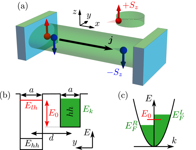
Figure 1: (a) QD side coupled to the quantum wire. The difference of the tunneling probabilities for spin-up (red balls with arrows) and spin-down (blue ones) holes from the quantum wire to the QD and of the spin flip rates leads to the current induced spin polarization in the QD. (b) Energy diagram and the geometric parameters of the system. (c) Heavy hole distribution function in the quantum wire. The light hole resonance energy $E_{0}$ is between the Fermi energies of the heavy holes in the quantum wire propagating from the left, $E_{F}^{L}$, and from the right, $E_{F}^{R}$, leads.

Most importantly, $V_{k,\pm}$ in Eq. (1) denote the tunneling matrix elements between the quantum wire and the QD. They are produced by the off-diagonal elements of the Luttinger Hamiltonian Luttinger (1956); Ivchenko (2005) and can be calculated as follows:

$$V_{k,\pm}=-\frac{\sqrt{3}\gamma_{2}\hbar^{2}}{2m_{0}}\left\langle\Phi_{\pm}|(k_{x}\mp{\rm i}k_{y})^{2}|\Psi_{k,\mp}\right\rangle,$$ (2)

where $\Phi_{\pm}$ denotes a localized light hole wave function of an isolated QD with the corresponding spin, $\Psi_{k,\pm}$ is a heavy hole wave function of an isolated quantum wire, $\gamma_{2}$ is the second Luttinger parameter (we use the spherical approximation), $m_{0}$ is the free electron mass, and $k_{\alpha}=-{\rm i}\partial/\partial\alpha$ with $\alpha=x,y$ are the components of the wave vector operator. It follows from the time reversal symmetry that $V_{k,\pm}=V_{-k,\mp}^{*}$. We note that the heavy hole mass along the wire is given by $m=m_{0}/(\gamma_{1}+\gamma_{2})$, where $\gamma_{1}$ is the first Luttinger parameter, and the dispersion is given by $E_{k}=\hbar^{2}k^{2}/(2m)$. We chose the state with $k=0$ to be the energy reference.

To be specific, let us consider the Gaussian wave functions sup :

$$\Phi_{\pm}\propto\exp\left(-\frac{x^{2}+(y-d)^{2}}{a^{2}}\right),$$ (3a)

$$\Psi_{k,\pm}\propto\exp\left({\rm i}kx-\frac{y^{2}}{a^{2}}\right),$$ (3b)

where $a$ is the localization length, which is assumed to be the same for the QD and the quantum wire and $d$ is the distance between the center of the QD and the wire axis, see Fig. 1(b). Assumption of the same localization length for the QD and the quantum wire greatly simplifies the analytical calculations and does not change the general results. With these wave functions the matrix elements $V_{k,\pm}$ are real and can be calculated analytically sup . They are shown in Fig. 2(a) as functions of the wave vector for $d/a=3$. One can see that for the given $k$ the tunneling matrix elements are generally strongly different for the spin-up and spin-down holes, which allows one to expect the high degree of the current induced spin polarization.

The single particle states of the Hamiltonian (1) are well known from the works of Anderson and Fano Anderson (1961); Fano (1961); Limonov et al. (2017). The coupling between the QD and the quantum wire leads to the formation of the quasi bound states at the energy $E_{0}$. Their chirality (also termed directionality) $\mathcal{C}$ can be defined as the difference of the probabilities for a light hole with a given spin to tunnel from the QD to the quantum wire states propagating to the right and to the left Lodahl et al. (2017); Spitzer et al. (2018); Overvig et al. (2021):

$$\mathcal{C}=\frac{V_{k_{0},+}^{2}-V_{-k_{0},+}^{2}}{V_{k_{0},+}^{2}+V_{-k_{0},+}^{2}},$$ (4)

where $k_{0}=\sqrt{2mE_{0}}/\hbar$. Due to the time reversal symmetry, the chirality is opposite for the two spin states, so the definition of its sign is ambiguous.

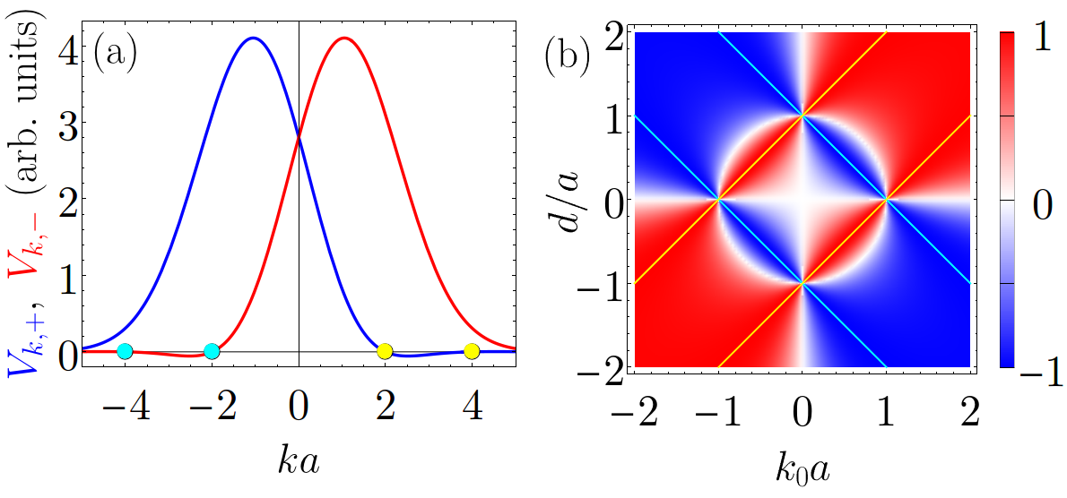
Figure 2: (a) Tunneling matrix elements calculated after Eq. (2) for $d=3a$. (b) Chirality $\mathcal{C}$ of the quasi bound state calculated after Eq. (4). The negative values of $d$ correspond to the location of the QD at the opposite side of the quantum wire.

The chirality of the quasi bound state is shown in Fig. 2(b) as a color map. The regions with $k_{0}<0$ and $d<0$ show that the chirality is odd under reflection in $(yz)$ and $(xz)$ planes, respectively. Generally, the absolute value of the chirality is of the order of unity. Moreover, it turns to unity exactly along the four lines given by the equation

$$k_{0}a=\pm d/a\pm 1,$$ (5)

which are shown by yellow and light blue in Fig. 2(b). At the corresponding QD energies one of the tunneling matrix elements vanishes, which is shown by yellow and light blue circles in Fig. 2(a). As a result, completely chiral bound states in the continuum are formed, so that the light hole state in the QD couples to the states in the wire propagating only in one direction. These completely chiral bound states in the continuum are robust and appear almost for any choice of the QD and the quantum wire wave functions, as we have checked. The Gaussian form of the wave functions (3) corresponds to the parabolic localization potential, so at $k_{0}a>2$ the coupling to the second size quantized subband of the quantum wire can play a role. Still in the most realistic region of $k_{0}a<2$ and $d/a\gtrsim 2$ the chirality is very close to unity.

II Formalism

To calculate the current induced spin polarization in the nonequilibrium steady state, we use the nonequilibrium Keldysh diagram technique Rammer and Smith (1986); Stefanucci and van Leeuwen (2013); Arseev (2015). We start from the bare Hubbard retarded Green’s function of an isolated QD Hubbard and Flowers (1963); Haug and Jauho (2008):

$$G_{0,\sigma}^{R}(\omega)=\frac{1-\left\langle n_{-\sigma}\right\rangle}{\omega-E_{0}+{\rm i}\delta},$$ (6)

where $\left\langle n_{\sigma}\right\rangle$ with $\sigma=\pm$ are the average occupancies of the corresponding light hole spin states, $\delta\to 0^{+}$, and we measure frequencies in the units of energy for brevity. Henceforth we focus on the limit of strong Coulomb repulsion (as compared with the quasi bound state width), while the general case is described in the Supplemental Material sup . Then using the standard self energy $\Sigma_{\sigma}^{R}(\omega)=\sum_{k}|V_{k,\sigma}^{2}|/(\omega-E_{k}+{\rm i}\delta)$ we obtain from the Dyson equation

$$G_{\sigma}^{R}(\omega)=\frac{1-\left\langle n_{-\sigma}\right\rangle}{\omega-E_{0}+{\rm i}(1-\left\langle n_{-\sigma}\right\rangle)\Gamma},$$ (7)

where $\Gamma=\pi D(E_{0})(V_{k_{0},+}^{2}+V_{k_{0},-}^{2})/4$ is the width of the quasi bound state with $D(E)=L\sqrt{2m/E}/(\pi\hbar)$ being the total density of states in the quantum wire. We assume $\Gamma$ to be much smaller than the band width $E_{1/a}$ and neglect the quasi bound state energy renormalization.

The occupancies of the QD states are given by the lesser Green’s function:

$$n_{\sigma}=-{\rm i}\int\frac{\mathrm{d}\omega}{2\pi}G_{\sigma}^{<}(\omega),$$ (8)

which in the steady state is given by $G_{\sigma}^{<}=G_{\sigma}^{R}\Sigma_{\sigma}^{<}G_{\sigma}^{A}$. Here the lesser self energy depends on the Fermi energies in the left and right leads attached to the quantum wire, $E_{F}^{L}$ and $E_{F}^{R}$, respectively:

$$\Sigma_{\sigma}^{<}(\omega)=\frac{\pi{\rm i}D(\omega)}{2}\left[V_{k_{0},\sigma}^{2}\theta(E_{F}^{L}-\omega)+V_{-k_{0},\sigma}^{2}\theta(E_{F}^{R}-\omega)\right],$$ (9)

where $\theta(\omega)$ is the Heaviside step function. Hence Eq. (8) yields

$$\left\langle n_{\sigma}\right\rangle=(1-\left\langle n_{-\sigma}\right\rangle)\left\{\frac{1+\sigma\mathcal{C}}{2\pi}\arctan\left[\frac{E_{F}^{L}-E_{0}}{(1-\left\langle n_{-\sigma}\right\rangle)\Gamma}\right]\right.\\ \left.+\frac{1-\sigma\mathcal{C}}{2\pi}\arctan\left[\frac{E_{F}^{R}-E_{0}}{(1-\left\langle n_{-\sigma}\right\rangle)\Gamma}\right]+\frac{1}{2}\right\}.$$ (10)

This set of two equations allows us to find self consistently the occupancies of the spin states $\left\langle n_{\sigma}\right\rangle$. Ultimately, the degree of the current induced spin polarization in the QD is given by $P=(\left\langle n_{+}\right\rangle-\left\langle n_{-}\right\rangle)/(\left\langle n_{+}\right\rangle+\left\langle n_{-}\right\rangle)$.

We note that this approach is valid on one hand for the temperatures below $\Gamma$, when the heavy holes distribution functions in the leads can be approximated by the step functions. On the other hand, the temperature is assumed to be larger than the Kondo temperature $T_{K}$, so that the high order correlations between holes can be neglected Haug and Jauho (2008). In fact the retarded Green’s function (7) without quasi bound state width renormalization can be obtained from the equations of motion in the Hartree-Fock approximation Lacroix (1981). The Kondo effect at low temperatures can be taken into account, for example, using equations of motion truncated in an appropriate way at the temperatures of the order of $T_{K}$ Meir et al. (1993); Świrkowicz et al. (2003) or much smaller than it Lacroix (1981). We expect that the Kondo effect would lead to the enhancement of the Coulomb blockade of one spin state by another, which would lead to the increase of the current induced spin polarization.

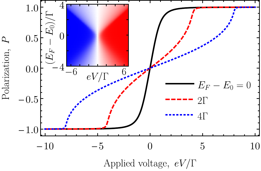
Figure 3: Current induced spin polarization in the chiral bound state, $\mathcal{C}=1$, as a function of the applied bias for the different Fermi levels $E_{F}-E_{0}$. The inset shows the spin polarization as a color map with the blue and red colors corresponding to $P=-1$ and $1$, respectively.

III Results

It follows from Eq. (10) that the chirality of the quasi bound state $\mathcal{C}$ produces explicit spin dependence of the occupancies provided a nonzero bias $eV=E_{F}^{L}-E_{F}^{R}$ is applied to the quantum wire. The current induced spin polarization is plotted in Fig. 3 as a function of bias for the different positions of the Fermi energy $E_{F}=(E_{F}^{L}+E_{F}^{R})/2$ for the completely chiral quasi bound state, $\mathcal{C}=1$. Generally, it is an odd function of the applied voltage and for the large voltages its absolute value reaches 100%. For the resonant case, $E_{F}=E_{0}$, the spin polarization saturates at $eV\sim\Gamma$ and for the detuned case it saturates at $eV\sim 2|E_{F}-E_{0}|$, as clearly seen from the inset in Fig. 3. Generally, the current induced spin polarization is the largest when the energy of the quasi bound state $E_{0}$ lies between the Fermi energies of the left and right leads, as it is shown in Fig. 1(c). For $\mathcal{C}<1$ the shape of this dependence is qualitatively the same.

Thus the large spin polarization can be induced by the voltages of the order of $\Gamma$, which is exponentially small being proportional to the squared tunneling matrix elements. The ultimate limit for it is set by the spin relaxation time in the isolated QD. In the absence of magnetic field, the nuclear spin fluctuations lead to the spin relaxation at the nanosecond time scale Glazov (2018); Smirnov et al. (2020), which corresponds to $\Gamma\sim 1~{}\mu$eV. However, to achieve this giant spin sensitivity the temperature of the system should be as low as a few millikelvins.

The spin polarization in the limit of large bias can be found from Eq. (10) by setting the first arctangent to $\pi/2$ and the second one to $-\pi/2$. This gives

$$P_{\rm max}=\frac{2\mathcal{C}}{\mathcal{C}^{2}+1},$$ (11)

which is determined solely by the chirality of the quasi bound state. The maximum spin polarization degree is shown in Fig. 4 as a function of the quasi bound state energy for different distances between the QD and the quantum wire. Here the range of $E_{0}<4\mathcal{E}$ with $\mathcal{E}=\hbar^{2}/(2ma^{2})$ corresponds to the energies below the bottom of the second size quantized band of the quantum wire. Generally, the maximum spin polarization decreases with increase of the distance between the quantum wire and the QD because of the chirality decrease shown in Fig. 2(b). However, it is still close to unity almost in the whole range of the quasi bound state energies $E_{0}$ up to $d\sim 10a$. We note that this corresponds to the suppression of the quasi bound state width by a giant factor of $\mathrm{e}^{d^{2}/a^{2}}$. The inset in Fig. 4 explicitly shows the range of the parameters where the current induced spin polarization at the large bias exceeds 90%.

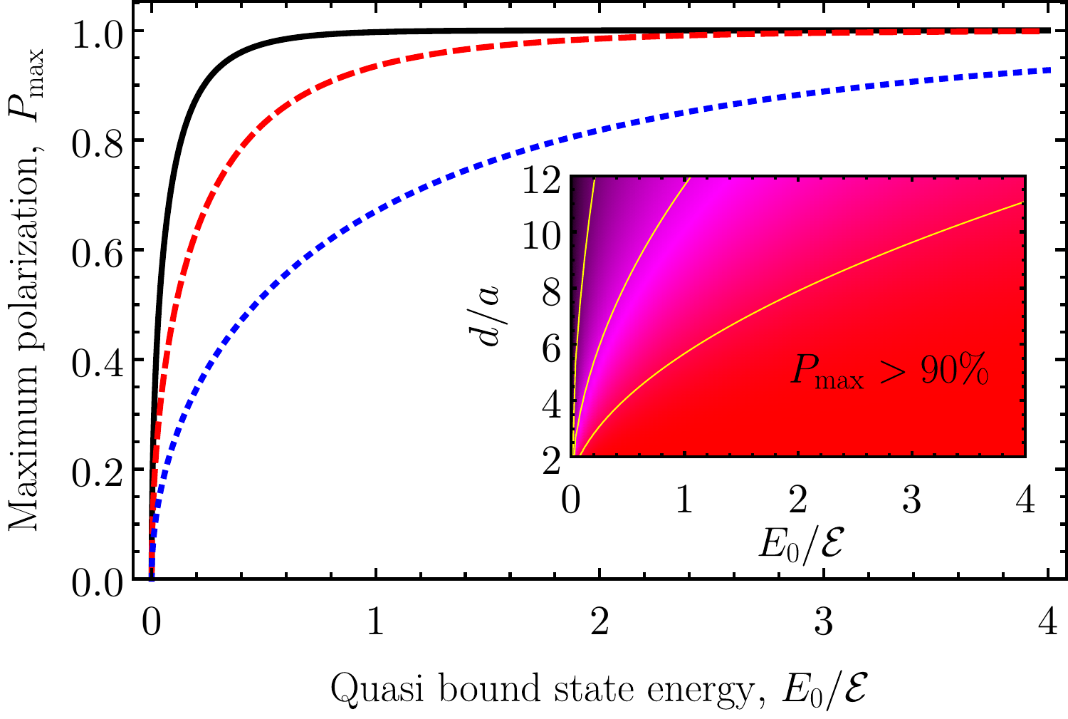
Figure 4: Spin polarization in the limit of the large bias as a function of the quasi bound state energy for $d/a=3$ (black solid curve), $5$ (red dashed curve), and $10$ (blue dotted curve). The inset shows the same as a color map. The yellow curves show the levels of $P_{\rm max}=0.3$, $0.6$ and $0.9$.

IV Discussion

The current induced spin polarization can be directly detected optically using the spin-induced Faraday rotation at the resonances related, for example, with the trion optical transitions in the QD. Alternatively, the spin polarization can be detected electrically using ferromagnetic contacts including magnetic microscope tips or using an additional QD weakly coupled to the main one due to the spin blockade effect and exchange interaction between the two QDs Hanson et al. (2007). There is also an inverse effect: the spin generation in the QD by external means would lead to the spin galvanic effect, e.g. to the current in the wire, which can be measured directly.

We note also that if the two QDs are placed at the opposite sides of the quantum wire, the electric current produces the opposite spin polarizations in them similarly to the spin Hall effect, as can be seen from the chirality shown in Fig. 2(b). However, for a single QD the hole spin flips are more efficient in one direction then in the opposite, so the total spin polarization of holes in the system is nonzero in contrast with the spin Hall effect.

We stress that the proposed mechanism of the current induced spin polarization via the chiral quasi bound states does not require magnetic field or linear in momentum spin-orbit coupling in contrast to the previous approaches. The spin-orbit interaction required here describes the splitting of the valence band exactly at the center of the Brillouin zone. It results in the off-diagonal matrix elements of the Luttinger Hamiltonain [see Eq. (2)], which are related to the diagonal ones as $\gamma_{2}/\gamma_{1}$. We stress that this ratio is not parametrically small and amounts, for example, to $0.28$, $0.08$, and $0.32$ in GaAs, Si and Ge, respectively. The close to unity spin polarization is equally possible in all these materials.

In conclusion, we demonstrated that the complex valence band structure leads to the chirality of the quasi bound states of the light holes in the QD side-coupled to the quantum wire with the heavy holes. The current flowing along the quantum wire produces nonequilibrium spin polarization of holes in the QD. This new mechanism of the current induced spin polarization has the following advantages: (i) It takes place for the exponentially small applied voltages. (ii) It does not require magnetic field and can be applied to the centrosymmetric materials. (iii) In the broad range of the geometric parameters the current induced spin polarization reaches 100%.

We thank L. E. Golub, M. M. Glazov, and I. V. Krainov for fruitful discussions. We acknoledge RF President Grant No. MK-5158.2021.1.2 and the Foundation for the Advancement of Theoretical Physics and Mathematics “BASIS”. Analytical calculations by D.S.S were supported by the Russian Science Foundation grant No. 19-12-00051. V.N.M. acknowledges support by RFBR grant ($20-32-70001$ Stability) and support from the Interdisciplinary Scientific and Educational School of Moscow University “Photonic and Quantum technologies. Digital medicine”.

The Supplementary Material includes the following topics:

toc

Appendix A S1. Hamiltonian and matrix elements

The Hamiltonian of the quantum dot (QD) with light holes side-coupled to the quantum wire with heavy holes can be written as follows [Eq. (1) in the main text]:

$$\mathcal{H}=E_{0}\sum_{\pm}n_{\pm}+Un_{+}n_{-}+\sum_{k,\pm}E_{k}n_{k,\pm}\\ +\sum_{k,\pm}\left(V_{k,\pm}d_{\pm}^{\dagger}c_{k,\mp}+{\rm H.c.}\right).$$ (S1)

We recall that $n_{\pm}=d_{\pm}^{\dagger}d_{\pm}$ are the occupancies of the light holes states in the QD having the spins $J_{z}=\pm 1/2$ with $d_{\pm}$ ($d_{\pm}^{\dagger}$) being the corresponding annihilation (creation) operators, $E_{0}$ is the energy of the light hole states in the QD which includes the interaction with the lower lying occupied heavy hole states in the QD, $U$ is the Coulomb repulsion energy between the two light hole states, $n_{k,\pm}=c_{k,\pm}^{\dagger}c_{k,\pm}$ are the occupancies of the heavy hole states in the quantum wire with the wave vector $k$ and spin $J_{z}=\pm 3/2$ with $c_{k,\pm}$ ($c_{k,\pm}^{\dagger}$) being the corresponding annihilation (creation) operators, and, finally, $V_{k,\pm}$ are the tunneling matrix elements.

The tunneling matrix elements $V_{k,\pm}$ can be calculated using the Luttinger Hamiltonian, which in the hole representation has the form Ivchenko (2005):

$$\mathcal{H}_{L}=\left(\begin{array}[]{cccc}F&H&I&0\\ H^{*}&G&0&I\\ I^{*}&0&G&-H\\ 0&I^{*}&-H^{*}&F\end{array}\right).$$ (S2)

It is written in the basis of the spin states $J_{z}=+3/2,+1/2,-1/2,-3/2$ and has the elements

$$F = \frac{\hbar^{2}(\gamma_{1}-2\gamma_{2})}{2m_{0}}k_{z}^{2}+\frac{\hbar^{2}(\gamma_{1}+\gamma_{2})}{2m_{0}}(k_{x}^{2}+k_{y}^{2}),$$

$$G = \frac{\hbar^{2}(\gamma_{1}+2\gamma_{2})}{2m_{0}}k_{z}^{2}+\frac{\hbar^{2}(\gamma_{1}-\gamma_{2})}{2m_{0}}(k_{x}^{2}+k_{y}^{2}),$$

$$H = -\frac{\sqrt{3}\hbar^{2}\gamma_{2}}{m_{0}}k_{z}(k_{x}-ik_{y}),$$

$$I = -\frac{\sqrt{3}\hbar^{2}}{2m_{0}}\left[\gamma_{2}(k_{x}^{2}-k_{y}^{2})-2i\gamma_{3}k_{x}k_{y}\right],$$ (S3)

where $m_{0}$ is the free electron mass, $\gamma_{1,2,3}$ are the Luttinger parameters and $\bm{k}$ is the hole wave vector. We use the spherical approximation $\gamma_{2}=\gamma_{3}$, so the Hamiltonian takes the form

$$\mathcal{H}_{L}=\frac{\hbar^{2}k^{2}}{2m_{0}}\left(\gamma_{1}+\frac{5}{2}\gamma_{2}\right)-\frac{\hbar^{2}\gamma_{2}}{m_{0}}(\bm{kJ})^{2},$$ (S4)

where $\bm{J}$ is the hole spin. In this case the energy of the heavy hole states in the quantum wire reads

$$E_{k}=\frac{\hbar^{2}k^{2}}{2m}$$ (S5)

with $m=m_{0}/(\gamma_{1}+\gamma_{2})$ being the heavy hole mass along the wire.

Let $\hat{\Psi}_{k,\pm}=\Psi_{k,\pm}\chi_{\pm 3/2}$ be the heavy hole wave function in the quantum wire with the wave vector $k$ along the wire and the spin $J_{z}=\pm 3/2$ and $\hat{\Phi}_{\pm}=\Phi_{\pm}\chi_{\pm 1/2}$ be the light hole wave function in the QD with the spin $J_{z}=\pm 1/2$, respectively, where $\chi_{J_{z}}$ are the spinors. The tunneling matrix elements between them involve the change of the spin, which can not be provided by the external electrostatic potential. Instead, it is produced by the Luttinger Hamiltonian:

$$V_{k_{\pm}}=\left\langle\hat{\Phi}_{\pm}|\mathcal{H}_{L}|\hat{\Psi}_{k,\mp}\right\rangle.$$ (S6)

We assume that structure is symmetric in the $(xy)$ plane containing the QD and the quantum wire, so the matrix elements between the states $\hat{\Phi}_{\pm}$ and $\hat{\Psi}_{k,\pm}$, respectively, being given by the $H$ term in the Luttinger Hamiltonian, which is proportional to $k_{z}$, vanish. As a result, the coupling takes place between the states $\hat{\Phi}_{\pm}$ and $\hat{\Psi}_{k,\mp}$ only. It is produced by the matrix element $I$ and involves the spin flip from $\mp 3/2$ to $\pm 1/2$, respectively.

To be specific, we consider the Gaussian wave functions [see Eqs. (3) in the main text]

$$\Phi_{\pm}=\varphi(z)\sqrt{\frac{2}{\pi}}\frac{1}{a}\exp\left(-\frac{x^{2}+(y-d)^{2}}{a^{2}}\right),$$ (S7a)

$$\Psi_{k,\pm}=-\psi(z)\sqrt{\frac{1}{aL}}\sqrt[4]{\frac{2}{\pi}}\exp\left({\rm i}kx-\frac{y^{2}}{a^{2}}\right).$$ (S7b)

Here we use the coordinate frame with the origin at the center of the quantum wire cross section, we choose the $x$ axis to be parallel to the quantum wire and the QD center to be located at the coordinates $(0,d,0)$, see Fig. S1. We assume the localization length $a$ to be the same for the QD and the quantum wire, $L$ is the normalization length, $\varphi(z)$ and $\psi(z)$ are the normalized wave functions along the growth axis $z$, and we assume the size quantization in this direction to be the strongest. The minus sign is introduced in Eq. (S7b) in order to get mostly positive tunneling matrix elements. We note that the matrix elements for the different localization lengths of the QD and the quantum wire can be also calculated analytically. However, we do not demonstrate it here since the corresponding expressions are cumbersome and all the physical effects do not change qualitatively.

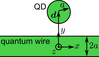
Figure S1: Geometry of the system and the coordinate frame.

For the wave functions (S7) the tunneling matrix elements read

$$V_{k,\pm}=\frac{\sqrt{3}\sqrt[4]{2\pi}\gamma_{2}\hbar^{2}V_{z}}{2m_{0}a\sqrt{La}}\left[\left(\frac{d}{a}\pm ka\right)^{2}-1\right]\\ \times\exp\left(-\frac{a^{2}k^{2}}{4}-\frac{d^{2}}{2a^{2}}\right),$$ (S8)

where $V_{z}=\left\langle\phi(z)|\psi(z)\right\rangle$. One can see, that the matrix elements are real. The matrix elements exponentially decay with the distance $d$ between the QD and the quantum wire. Most importantly they are different for the given $k$, as illustrated in Fig. 2(a) in the main text. We note that the wave function (S7b) corresponds to the harmonic localization potential across the quantum wire along the $y$ direction. In this case the energy of the state with the wave vector $k=2/a$ coincides with the bottom of the second size quantized subband, so we will consider below the states in the range of $ka<2$ only. In the same time, the ratio $d/a$ can be arbitrary large in the model, but in fact it should not be too large in order to observe the effects of the hole tunneling between the QD and the quantum wire. We stress, that the tunneling matrix elements $V_{k,\pm}$ involve hole spin flips, but contain $\gamma_{2}/\gamma_{1}$ as a factor describing the spin-orbit interaction only. This ratio is not small, so the current induced spin polarization in this system is not parametrically suppressed.

For the given energy of the light hole states in the QD $E_{0}$ and the corresponding wave vector $k_{0}=\sqrt{2mE_{0}}/\hbar$ the tunneling matrix elements are different $V_{k_{0},+}\neq V_{k_{0},-}$, which allows us to define chirality as follows [Eq. (4) in the main text] Lodahl et al. (2017); Spitzer et al. (2018); Overvig et al. (2021):

$$\mathcal{C}=\frac{V_{k_{0},+}^{2}-V_{k_{0},-}^{2}}{V_{k_{0},+}^{2}+V_{k_{0},-}^{2}}.$$ (S9)

We note that due to the mirror and time reversal symmetries

$$V_{k,\pm}=V_{-k,\mp},$$ (S10)

so the definition of the sign of $\mathcal{C}$ is arbitrary.

From Eq. (S8) we find the chirality

$$\mathcal{C}=\frac{4dk_{0}[(k_{0}a)^{2}+(d/a)^{2}-1]}{[(k_{0}a)^{2}-1]^{2}+6(dk_{0})^{2}-2(d/a)^{2}+(d/a)^{4}}.$$ (S11)

One can see that it is an odd function of $d$ and $k_{0}$ as shown in Fig. 2(b) in the main text. It vanishes at $d=0$ and $k=0$, as expected, and also at $(d/a)^{2}+(ka)^{2}=1$. These lines are white in Fig. 2(b) in the main text. But most importantly the chirality reaches $\pm 1$ at [Eq. (5) in the main text]

$$k_{0}a=\pm d/a\pm 1,$$ (S12)

which is shown by yellow and light blue lines in Fig. 2(b) in the main text. Along these lines the current induced spin polarization can reach exactly $100\%$, as we demonstrate in the main text. We note that the corresponding energy $E_{0}$ can be found for any $d$, and we checked that this holds for a broad class of the wave functions apart from Eqs. (S7).

Appendix B S2. General formalism for current induced spin polarization

Here we calculate the current induced spin polarization in the QD produced by the nonequilibrium distribution functions of the heavy holes in the quantum wire inherited from the attached leads. We assume that the occupancies of the states in the quantum wire are given by

$$\left\langle n_{k}\right\rangle=\theta(E_{k})\left[\theta(E_{F}^{L}-E_{k})\theta(k)+\theta(E_{F}^{R}-E_{k})\theta(-k)\right],$$ (S13)

where $E_{F}^{L}$ and $E_{F}^{R}$ are the Fermi energies in the left and right leads, respectively, and $\theta(t)$ is the Heaviside step function. This distribution is relevant for the temperatures below the width of the quasi bound state.

At the first step, we neglect tunneling and use equations of motion to obtain the retarded Hubbard Green’s function of the QD Hubbard and Flowers (1963); Haug and Jauho (2008) [c.f. Eq. (6) in the main text]:

$$G_{0,\sigma}^{R}(\omega)=\frac{1-\left\langle n_{-\sigma}\right\rangle}{\omega-E_{0}+{\rm i}\delta}+\frac{\left\langle n_{-\sigma}\right\rangle}{\omega-E_{0}-U+{\rm i}\delta},$$ (S14)

where we set $\hbar=1$ for brevity. We recall that it is defined as the Fourier transform of $-{\rm i}\left\langle\left\{d_{\sigma}^{\dagger}(0),d_{\sigma}(t)\right\}\right\rangle\theta(t)$. The average occupancies of the light hole spin states $\left\langle n_{\sigma}\right\rangle$ should be determined self consistently taking into account the tunneling processes.

Figure S1: Dyson equation and the self energy for the tunneling problem. Thick solid, thin solid and dashed lines correspond to $G_{\sigma}(\omega)$, $G_{0,\sigma}(\omega)$, and $G_{k,-\sigma}(\omega)$, respectively.

Then we account for the tunneling as a perturbation while keeping the Fermi energies in the left and right leads, $E_{F}^{L}$ and $E_{F}^{R}$, different. This can be done in the Keldysh formalism Rammer and Smith (1986); Stefanucci and van Leeuwen (2013); Arseev (2015). The self energy in this problem is trivial, see Fig. S1, it reads

$$\Sigma_{\sigma}^{R}(\omega)=\sum_{k}|V_{k,\sigma}^{2}|G_{k,-\sigma}^{R}(\omega),$$ (S15)

where

$$G_{k,\sigma}^{R}(\omega)=\frac{1}{\omega-E_{k}+{\rm i}\delta}$$ (S16)

is the retarded Green’s function of heavy holes in the quantum wire. We note that the tunneling in Eq. (S1) flips the spin $\sigma$. From the Dyson equation, Fig. S1, we obtain

$$G_{\sigma}^{R}(\omega)=\frac{G_{0,\sigma}^{R}(\omega)}{1-G_{0,\sigma}^{R}(\omega)\Sigma_{\sigma}^{R}(\omega)}.$$ (S17)

We note that the retarded self energy $\Sigma_{\sigma}^{R}(\omega)$ in Eq. (S15) diverges at $\omega=-{\rm i}\delta$ and as a result one obtains a pole in $G_{\sigma}^{R}(\omega)$ at small negative real $\omega$, which corresponds to the truly bound state. This state is generally present in the one dimensional problems with an impurity. We will assume that $E_{0}$ is large enough and will neglect the contribution of the true bound state to the current induced spin polarization. In this case, in the steady state the lesser Green’s function defined as the Fourier transform of ${\rm i}\left\langle d_{\sigma}^{\dagger}d_{\sigma}(t)\right\rangle$ is given by

$$G_{\sigma}^{<}(\omega)=G_{\sigma}^{R}(\omega)\Sigma_{\sigma}^{<}(\omega)G_{\sigma}^{A}(\omega),$$ (S18)

where $G_{\sigma}^{A}(\omega)=[G_{\sigma}^{R}(\omega)]^{*}$ is the advanced Green’s function and $\Sigma_{\sigma}^{<}(\omega)$ is the lesser self energy given by

$$\Sigma_{\sigma}^{<}(\omega)=\sum_{k}|V_{k,\sigma}^{2}|G_{k,-\sigma}^{<}(\omega),$$ (S19)

as follows from Fig. S1. The lesser Green’s functions of the holes in the quantum wire are determined by the occupancies of the states:

$$G_{k,\sigma}^{<}(\omega)=2\pi{\rm i}\left\langle n_{k}\right\rangle\delta(\omega-E_{k}),$$ (S20)

which are defined by the Fermi energies in the leads, see Eq. (S13). This gives the lesser self energy

$$\Sigma_{\sigma}^{<}(\omega)=2{\rm i}\left[\Gamma_{L,\sigma}(\omega)n_{L}(\omega)+\Gamma_{R,\sigma}(\omega)n_{R}(\omega)\right],$$ (S21)

where

$$\Gamma_{L/R,\sigma}(\omega)=\pi\frac{D(\omega)}{4}V_{+k_{\omega}/-k_{\omega},\sigma}^{2}$$ (S22)

are the tunneling rates with $D(\omega)=(L/\pi)\sqrt{2m/\omega}$ being the total density of states in the quantum wire including spin, $n_{L/R}(\omega)=\left\langle n_{+k_{\omega}/-k_{\omega}}\right\rangle$, and $k_{\omega}=\sqrt{2m\omega}$. We note that $\Gamma(\omega)=\Gamma_{L,\sigma}(\omega)+\Gamma_{R,\sigma}(\omega)$ determines the widths of the quasi bound states according to:

$$-\mathop{\rm Im}\left[\Sigma_{\sigma}^{R}(\omega)\right]=\Gamma(\omega),$$ (S23)

where we used Eq. (S15). It does not depend on spin, as follows from Eq. (S10). The tunneling rates $\Gamma_{L/R,\sigma}(\omega)$ can be also obtained from the Fermi golden rule.

Finally, the occupancies of the spin states in the QD $\left\langle n_{\pm}\right\rangle$ should be found self consistently as

$$\left\langle n_{\sigma}\right\rangle=-{\rm i}\int\limits_{-\infty}^{\infty}G_{\sigma}^{<}(\omega)\frac{\mathrm{d}\omega}{2\pi},$$ (S24)

where the lesser Green’s function is given by Eq. (S18) with the lesser self energy from Eq. (S21) and retarded and advanced Green’s functions from Eq. (S17), which includes the same occupancies of the spin states through the Hubbard Green’s function, Eq. (S14).

Ultimately, the spin polarization in the QD is given by

$$P=\frac{\left\langle n_{+}\right\rangle-\left\langle n_{-}\right\rangle}{\left\langle n_{+}\right\rangle+\left\langle n_{-}\right\rangle}.$$ (S25)

Below we consider the limits of zero and infinite Coulomb interaction and use the wide band approximation to obtain simplified expressions for the current induced spin polarization.

Appendix C S3. Weak Coulomb interaction

Here for the purpose of illustration we consider the simple limit of $U=0$, when the interaction between the holes in the QD can be neglected. In this limit the bare Green’s function of the QD, Eq. (S14), reduces to

$$G_{0,\sigma}^{R}(\omega)=\frac{1}{\omega-E_{0}+{\rm i}\delta}.$$ (S26)

Thus from Eq. (S17) we obtain

$$G_{\sigma}^{R}(\omega)=\frac{1}{\omega-\tilde{E}_{0}(\omega)+{\rm i}\Gamma(\omega)},$$ (S27)

where

$$\tilde{E}_{0}(\omega)=E_{0}+\mathop{\rm Re}\left[\Sigma_{\sigma}^{R}(\omega)\right]$$ (S28)

is the energy of the quasi bound state in the QD. Substituting it in Eq. (S18) and Eq. (S24) along with Eq. (S21) we obtain the occupancies of the spin states

$$\left\langle n_{\pm}\right\rangle=\int\limits_{0}^{\infty}\frac{2\Gamma(\omega)n_{\pm}(\omega)}{\left[\omega-\tilde{E}_{0}(\omega)\right]^{2}+\Gamma^{2}(\omega)}\frac{\mathrm{d}\omega}{2\pi},$$ (S29)

where

$$n_{\pm}(\omega)=\frac{\Gamma_{L,\pm}(\omega)n_{L}(\omega)+\Gamma_{R,\pm}(\omega)n_{R}(\omega)}{\Gamma(\omega)}.$$ (S30)

One can obtain the same result for the limit of negligible Coulomb interaction from the exact solution of a single particle problem. To explicitly demonstrate this, we consider the single particle eigenfunctions of the Hamiltonian (S1) with $U=0$. They can be found following, for example, the original work of Fano [Fano, 1961]. For the given energy $E>0$ and spin $\sigma$ of the light hole state, the two energy degenerate wave functions have the form

$$\Psi_{1,2}^{\sigma}=a_{1,2}\Phi_{\sigma}+{\rm v.p.}\int\limits_{0}^{\infty}\mathrm{d}E^{\prime}\left[b_{1,2}^{\sigma}(E^{\prime})\Psi_{k^{\prime},-\sigma}\right.\\ \left.+c_{1,2}^{\sigma}(E^{\prime})\Psi_{-k^{\prime},-\sigma}\right],$$ (S31)

where the coefficients are

$$a_{1}=\frac{4\sin(\Delta)}{\pi D(E)Y_{E}},$$ (S32a)

$$b_{1}^{\sigma}(E^{\prime})=\frac{V_{k^{\prime},\sigma}}{Y_{E}}\left[\frac{1}{\pi}\frac{\sin(\Delta)}{E-E^{\prime}}-\cos(\Delta)\delta(E-E^{\prime})\right],$$ (S32b)

$$c_{1}^{\sigma}(E^{\prime})=\frac{V_{-k^{\prime},\sigma}}{Y_{E}}\left[\frac{1}{\pi}\frac{\sin(\Delta)}{E-E^{\prime}}-\cos(\Delta)\delta(E-E^{\prime})\right],$$ (S32c)

$$a_{2}=0,$$ (S33a)

$$b_{2}^{\sigma}(E^{\prime})=\frac{V_{-k^{\prime},\sigma}}{Y_{E}}\delta(E-E^{\prime}),$$ (S33b)

$$c_{2}^{\sigma}(E^{\prime})=-\frac{V_{k^{\prime},\sigma}}{Y_{E}}\delta(E-E^{\prime})$$ (S33c)

with the following parameters: $\Delta=\arctan[\Gamma/(\tilde{E}_{0}-E)]$, $Y_{E}=\sqrt{V_{k_{E},\sigma}^{2}+V_{-k_{E},\sigma}^{2}}$ (it does not depend on $\sigma$) and $k^{\prime}=\sqrt{2mE^{\prime}}$.

We note that

$$\tilde{E}_{0}=E_{0}+{\rm v.p.}\int\limits_{0}^{\infty}\mathrm{d}E^{\prime}\frac{D(E^{\prime})Y_{E^{\prime}}^{2}}{4(E-E^{\prime})}$$ (S34)

and

$$\Gamma=\pi\frac{D(E)Y_{E}^{2}}{4}$$ (S35)

in agreement with Eq. (S15): $\Sigma_{\sigma}^{R}(E)=\tilde{E}_{0}-E_{0}-{\rm i}\Gamma$.

We also note that these eigenfunctions do not form a complete set, because any potential in one dimensional problem produces a bound state with a negative energy $E_{b}<0$. The two Kramers degenerate truly localized states have the same form of Eq. (S31):

$$\Psi_{0}^{\sigma}=a_{0}^{\sigma}\Phi_{\sigma}+{\rm v.p.}\int\limits_{0}^{\infty}\mathrm{d}E^{\prime}\left[b_{0}^{\sigma}(E^{\prime})\Psi_{k^{\prime},-\sigma}\right.\\ \left.+c_{0}^{\sigma}(E^{\prime})\Psi_{-k^{\prime},-\sigma}\right].$$ (S36)

Here the coefficients have the form

$$b_{0}^{\sigma}(E^{\prime})=\frac{D(E^{\prime})a_{0}V_{k^{\prime}}^{\sigma}}{4(E_{b}-E^{\prime})},\qquad c_{0}^{\sigma}(E^{\prime})=\frac{D(E^{\prime})a_{0}V_{-k^{\prime}}^{\sigma}}{4(E_{b}-E^{\prime})},$$ (S37)

and the coefficient $a_{0}$ should be determined from the normalization of these wave functions. The energy of these truly bound states can be found from the relation

$$E_{b}=E_{0}+\int_{0}^{\infty}\frac{D(E^{\prime})Y_{E^{\prime}}^{2}}{4(E_{b}-E^{\prime})}.$$ (S38)

One can see that the Green’s function (S27) indeed has a pole at this energy. However, for $E_{0}\gg\Gamma$ this state is almost delocalized, $a_{0}^{\sigma}\ll 1$, so the contribution of this state can be neglected.

For the simple Gaussian wave functions (S7) and matrix elements (S8) one can readily find the width of the quasi bound state

$$\Gamma=\frac{3\sqrt{\pi}\gamma_{2}^{2}\hbar^{2}mV_{z}^{2}}{2\sqrt{2}a^{2}m_{0}^{2}}\left[a^{3}k_{E}^{3}+2(3d^{2}/a^{2}-1)k_{E}a\right.\\ \left.+(d^{2}/a^{2}-1)^{2}/(k_{E}a)\right]\exp\left(-k_{E}^{2}a^{2}/2-d^{2}/a^{2}\right).$$ (S39)

For the energy renormalization we obtain

$$\tilde{E}-E_{0}=\frac{3\gamma_{2}^{2}\hbar^{2}mV_{z}^{2}}{2\sqrt{2}a^{2}m_{0}^{2}}\left\{2\left[(k_{E}a)^{3}+2k_{E}a(3d^{2}/a^{2}-1)\right.\right.\\ \left.+(d^{2}/a^{2}-1)^{2}/(k_{E}a)\right]\mathcal{D}(k_{E}a/\sqrt{2})\\ \left.+\sqrt{2}\left[1-6(d/a)^{2}-(k_{E}a)^{2}\right]\right\}\exp\left(-d^{2}/a^{2}\right),$$ (S40)

where $\mathcal{D}(x)=e^{-x^{2}}\int_{0}^{x}\mathrm{e}^{y^{2}}\mathrm{d}y$ is the Dawson function. We remind that $k_{E}=\sqrt{2mE}/\hbar$ is used for brevity, and here we recovered the reduced Plank constant.

To describe the population of the QD spin states in the presence of the current, we consider the following linear combinations of the eigenfunctions at the given energy:

$$\Psi_{L}^{\sigma}=\frac{1}{Y_{E}}\left[V_{-k_{E},\sigma}\Psi_{2}^{\sigma}-V_{k_{E},\sigma}\mathrm{e}^{{\rm i}\Delta}\Psi_{1}^{\sigma}\right],$$ (S41a)

$$\Psi_{R}^{\sigma}=\frac{1}{Y_{E}}\left[V_{k_{E},\sigma}\Psi_{2}^{\sigma}+V_{-k_{E},\sigma}\mathrm{e}^{{\rm i}\Delta}\Psi_{1}^{\sigma}\right].$$ (S41b)

These wave functions have the asymptotic behaviour $\Psi_{L/R}^{\sigma}\propto\exp(\pm{\rm i}k_{E}x)$ for $x\to\pm\infty$, respectively. Thus they describe the heavy hole states propagating from the left and right leads, respectively.

The weight of the QD state in these functions is Anderson (1961)

$$|a_{L/R,\sigma}^{2}|=\frac{V_{\pm k_{E},\sigma}^{2}}{(E-\tilde{E}_{0})^{2}+\Gamma^{2}}.$$ (S42)

For the given Fermi energies $E_{F}^{L}$ and $E_{F}^{R}$ in the leads (and low temperatures) the occupancies of the QD states can be found as

$$\left\langle n_{\sigma}\right\rangle=\int\limits_{0}^{E_{F}^{L}}|a_{L,\sigma}^{2}|\frac{D(E)}{4}\mathrm{d}E+\int\limits_{0}^{E_{F}^{R}}|a_{R,\sigma}^{2}|\frac{D(E)}{4}\mathrm{d}E,$$ (S43)

which coincides with Eq. (S29) obtained in the Keldysh formalism.

The tunneling matrix elements are exponentially suppressed by the fast decay of the hole wave functions away from the QD and the quantum wire. So typically the width of the resonance $\Gamma$ is much smaller than its energy $E_{0}$. In this case one can use the wide band approximation and neglect the energy dependence of $D(E)$ and $V_{\pm k_{E},\sigma}$. Then Eq. (S43) yields

$$\left\langle n_{\pm}\right\rangle=\frac{1}{2}+\frac{1\pm\mathcal{C}}{2\pi}\arctan\left(\frac{E_{F}^{L}-\tilde{E}_{0}}{\Gamma}\right)\\ +\frac{1\mp\mathcal{C}}{2\pi}\arctan\left(\frac{E_{F}^{R}-\tilde{E}_{0}}{\Gamma}\right),$$ (S44)

where the chirality $\mathcal{C}$ is defined in Eq. (S9), while the quasi bound state energy $\tilde{E}_{0}$ and width $\Gamma$ are assumed to be taken at the energy $E_{0}$.

One can see that the polarization is the largest in the limit of large bias $E_{F}^{L}-E_{0},E_{0}-E_{F}^{R}\gg\Gamma$. In this limit one has $\left\langle n_{\pm}\right\rangle=(1\pm\mathcal{C})/2$, which yields the polarization

$$P=\mathcal{C}.$$ (S45)

So the chirality directly defines the largest current induced spin polarization without interaction.

We note that the limit of the large bias can be also described using the phenomenological kinetic equations

$$\frac{\mathrm{d}n_{\pm}}{\mathrm{d}t}=2\Gamma_{L,\pm}-2\Gamma n_{\pm},$$ (S46)

which describe the tunneling of the light holes to the QD with the rate $2\Gamma_{L,\pm}$ and out of the QD with the rate $2\Gamma$. In the steady state one obtains once again $n_{\pm}=\Gamma_{L,\pm}/\Gamma=(1\pm\mathcal{C})/2$ and Eq. (S45) in agreement with the Keldysh formalism and exact Hamiltonian diagonalization.

Appendix D S4. Strong Coulomb interaction

For small quantum dots it is relevant to consider the limit of strong Coulomb interaction, $U\to\infty$. In this limit one can neglect the second term in Eq. (S14) for the retarded bare Green’s function $G_{0,\sigma}^{R}(\omega)$ [Eq. (6) in the main text]:

$$G_{0,\sigma}^{R}(\omega)=\frac{1-\left\langle n_{-\sigma}\right\rangle}{\omega-E_{0}+{\rm i}\delta}.$$ (S47)

Similarly to the previous subsection we obtain the dressed retarded Green’s function

$$G_{\sigma}^{R}(\omega)=\frac{1-\left\langle n_{-\sigma}\right\rangle}{\omega-E_{0,\sigma}(\omega)+{\rm i}\Gamma_{\sigma}(\omega)},$$ (S48)

where $E_{0,\sigma}(\omega)=\left\langle n_{-\sigma}\right\rangle E_{0}+(1-\left\langle n_{-\sigma}\right\rangle)\tilde{E}_{0}(\omega)$ and $\Gamma_{\sigma}(\omega)=(1-\left\langle n_{-\sigma}\right\rangle)\Gamma(\omega)$. Thus we obtain the suppressed amplitude of the Green’s function, smaller renormalization of the energy of the quasi bound state, and its smaller width as compared with Eq. (S27).

Further, the occupancies of the QD spin states can be found from Eq. (S24) and (S18). In the wide band approximation in analogy with Eq. (S44) we obtain

$$\left\langle n_{\sigma}\right\rangle=(1-\left\langle n_{-\sigma}\right\rangle)\left[\frac{1}{2}+\frac{1+\sigma\mathcal{C}}{2\pi}\arctan\left(\frac{E_{F}^{L}-\tilde{E}_{0,\sigma}}{\Gamma_{\sigma}}\right)\right.\\ \left.+\frac{1-\sigma\mathcal{C}}{2\pi}\arctan\left(\frac{E_{F}^{R}-\tilde{E}_{0,\sigma}}{\Gamma_{\sigma}}\right)\right].$$ (S49)

This represents the set of two equations for $\left\langle n_{\pm}\right\rangle$, which should be solved self consistently.

In the limit of large bias $E_{F}^{L}-E_{0},E_{0}-E_{F}^{R}\gg\Gamma$ one obtains

$$\left\langle n_{\sigma}\right\rangle=(1-\left\langle n_{-\sigma}\right\rangle)(1+\sigma\mathcal{C})/2,$$ (S50)

which yields [Eq. (11) in the main text]:

$$P_{\rm max}=\frac{2\mathcal{C}}{1+\mathcal{C}^{2}}.$$ (S51)

Thus for the chiral quasi bound state, $\mathcal{C}=\pm 1$, in the presence of the interaction the current induced spin polarization reaches 100%.

This limit can be again described using the phenomenological kinetic equations

$$\frac{\mathrm{d}n_{\sigma}}{\mathrm{d}t}=2\Gamma_{L,\sigma}(1-n_{-\sigma})-2\Gamma n_{\sigma},$$ (S52)

which is similar to Eq. (S46), but accounts for the Coulomb blockade effect. These equations lead to

$$n_{\sigma}=\frac{(1\pm\mathcal{C})^{2}}{3+\mathcal{C}^{2}},$$ (S53)

which yields again Eq. (S51).

Generally, one can see that the Coulomb interaction increases the polarization degree. Qualitatively, this happens because the presence of a light hole with the given spin in the QD prevents tunneling of the hole with the opposite spin to the QD. As a result the spin polarization degree increases by a factor of $2/(1+\mathcal{C}^{2})$.

It follows from Eq. (S51) that it is enough to have quite a moderate chirality $|\mathcal{C}|>(10-\sqrt{19})/9\approx 0.63$ to obtain the spin polarization degree $P_{\rm max}$ larger then $90$%. The corresponding region of the system parameters is shown in the inset in Fig. 4 in the main text.

References

- Dyakonov (2020) M. I. Dyakonov, Will We Ever Have a Quantum Computer? (Springer Nature, 2020).
- Watson et al. (2018) T. F. Watson, S. G. J. Philips, E. Kawakami, D. R. Ward, P. Scarlino, M. Veldhorst, D. E. Savage, M. G. Lagally, M. Friesen, S. N. Coppersmith, M. A. Eriksson, and L. M. K. Vandersypen, A programmable two-qubit quantum processor in silicon, Nature 555, 633 (2018).
- Yoneda et al. (2018) J. Yoneda, K. Takeda, T. Otsuka, T. Nakajima, M. R. Delbecq, G. Allison, T. Honda, T. Kodera, S. Oda, Y. Hoshi, N. Usami, K. M. Itoh, and S. Tarucha, A quantum-dot spin qubit with coherence limited by charge noise and fidelity higher than 99.9%, Nat. Nanotechnol. 13, 102 (2018).
- Yang et al. (2020) C. H. Yang, R. C. C. Leon, J. C. C. Hwang, A. Saraiva, T. Tanttu, W. Huang, J. Camirand Lemyre, K. W. Chan, K. Y. Tan, F. E. Hudson, K. M. Itoh, A. Morello, M. Pioro-Ladriére, A. Laucht, and A. S. Dzurak, Operation of a silicon quantum processor unit cell above one kelvin, Nature 580, 350 (2020).
- Nowack et al. (2007) K. C. Nowack, F. H. L. Koppens, Y. V. Nazarov, and L. M. K. Vandersypen, Coherent Control of a Single Electron Spin with Electric Fields, Science 318, 1430 (2007).
- Zajac et al. (2018) D. M. Zajac, A. J. Sigillito, M. Russ, F. Borjans, J. M. Taylor, G. Burkard, and J. R. Petta, Resonantly driven CNOT gate for electron spins, Science 359, 439 (2018).
- Basso Basset et al. (2019) F. Basso Basset, M. B. Rota, C. Schimpf, D. Tedeschi, K. D. Zeuner, S. F. Covre da Silva, M. Reindl, V. Zwiller, K. D. Jöns, A. Rastelli, and R. Trotta, Entanglement Swapping with Photons Generated on Demand by a Quantum Dot, Phys. Rev. Lett. 123, 160501 (2019).
- Mills et al. (2019) A. R. Mills, D. M. Zajac, M. J. Gullans, F. J. Schupp, T. M. Hazard, and J. R. Petta, Shuttling a single charge across a one-dimensional array of silicon quantum dots, Nat. Commun. 10, 1063 (2019).
- Qiao et al. (2021) H. Qiao, Y. P. Kandel, S. Fallahi, G. C. Gardner, M. J. Manfra, X. Hu, and J. M. Nichol, Long-Distance Superexchange between Semiconductor Quantum-Dot Electron Spins, Phys. Rev. Lett. 126, 017701 (2021).
- Carter et al. (2021) S. G. Carter, S. C. Badescu, A. S. Bracker, M. K. Yakes, K. X. Tran, J. Q. Grim, and D. Gammon, Coherent Population Trapping Combined with Cycling Transitions for Quantum Dot Hole Spins Using Triplet Trion States, Phys. Rev. Lett. 126, 107401 (2021).
- Ivchenko and Pikus (1978) E. L. Ivchenko and G. E. Pikus, New photogalvanic effect in gyrotropic crystals, JETP Lett. 27, 604 (1978).
- Vorob’ev et al. (1979) L. E. Vorob’ev, E. L. Ivchenko, G. E. Pikus, I. I. Farbshtein, V. A. Shalygin, and A. V. Shturbin, Optical activity in tellurium induced by a current, JETP Lett. 29, 441 (1979).
- Ganichev et al. (2006) S. D. Ganichev, S. N. Danilov, P. Schneider, V. V. Bel’kov, L. E. Golub, W. Wegscheider, D. Weiss, and W. Prettl, Electric current-induced spin orientation in quantum well structures, J. Magn. Magn. Mater. 300, 127 (2006).
- Silov et al. (2004) A. Y. Silov, P. A. Blajnov, J. H. Wolter, R. Hey, K. H. Ploog, and N. S. Averkiev, Current-induced spin polarization at a single heterojunction, Appl. Phys. Lett. 85, 5929 (2004).
- Kato et al. (2004) Y. K. Kato, R. C. Myers, A. C. Gossard, and D. D. Awschalom, Current-Induced Spin Polarization in Strained Semiconductors, Phys. Rev. Lett. 93, 176601 (2004).
- Norman et al. (2014) B. M. Norman, C. J. Trowbridge, D. D. Awschalom, and V. Sih, Current-Induced Spin Polarization in Anisotropic Spin-Orbit Fields, Phys. Rev. Lett. 112, 056601 (2014).
- Stepanov et al. (2014) I. Stepanov, S. Kuhlen, M. Ersfeld, M. Lepsa, and B. Beschoten, All-electrical time-resolved spin generation and spin manipulation in n-InGaAs, Appl. Phys. Lett. 104, 062406 (2014).
- Ganichev et al. (2012) S. D. Ganichev, M. Trushin, and J. Schliemann, Spin polarization by current in Handbook of Spin Transport and Magnetism, edited by E. Y, Tsymbal and I. Zutic, p. 487, (Chapman & Hall, Boca Raton, 2012).
- Golub and Ivchenko (2013) L. E. Golub and E. L. Ivchenko, Spin-dependent phenomena in semiconductors in strong electric fields, New J. Phys. 15, 125003 (2013).
- Smirnov and Golub (2017) D. S. Smirnov and L. E. Golub, Electrical Spin Orientation, Spin-Galvanic, and Spin-Hall Effects in Disordered Two-Dimensional Systems, Phys. Rev. Lett. 118, 116801 (2017).
- Huber et al. (2017) D. Huber, M. Reindl, Y. Huo, H. Huang, J. S. Wildmann, O. G. Schmidt, A. Rastelli, and R. Trotta, Highly indistinguishable and strongly entangled photons from symmetric GaAs quantum dots, Nat. Commun. 8, 15506 (2017).
- Chekhovich et al. (2020) E. A. Chekhovich, S. F. C. da Silva, and A. Rastelli, Nuclear spin quantum register in an optically active semiconductor quantum dot, Nat. nanotech. 15, 999 (2020).
- Najer et al. (2019) D. Najer, I. Söllner, P. Sekatski, V. Dolique, M. C. Löbl, D. Riedel, R. Schott, S. Starosielec, S. R. Valentin, A. D. Wieck, N. Sangouard, A. Ludwig, and R. J. Warburton, A gated quantum dot strongly coupled to an optical microcavity, Nature 575, 622 (2019).
- Veldhorst et al. (2015) M. Veldhorst, C. H. Yang, J. C. C. Hwang, W. Huang, J. P. Dehollain, J. T. Muhonen, S. Simmons, A. Laucht, F. E. Hudson, K. M. Itoh, A. Morello, and A. S. Dzurak, A two-qubit logic gate in silicon, Nature 526, 410 (2015).
- Mi et al. (2017) X. Mi, J. V. Cady, D. M. Zajac, P. W. Deelman, and J. R. Petta, Strong coupling of a single electron in silicon to a microwave photon, Science 355, 156 (2017).
- Borjans et al. (2020) F. Borjans, X. Croot, X. Mi, M. Gullans, and J. Petta, Resonant microwave-mediated interactions between distant electron spins, Nature 577, 195 (2020).
- Hao et al. (2010) X.-J. Hao, T. Tu, G. Cao, C. Zhou, H.-O. Li, G.-C. Guo, W. Y. Fung, Z. Ji, G.-P. Guo, and W. Lu, Strong and Tunable Spin-Orbit Coupling of One-Dimensional Holes in Ge/Si Core/Shell Nanowires, Nano Lett. 10, 2956 (2010).
- Kloeffel et al. (2011) C. Kloeffel, M. Trif, and D. Loss, Strong spin-orbit interaction and helical hole states in Ge/Si nanowires, Phys. Rev. B 84, 195314 (2011).
- Hendrickx et al. (2020) N. Hendrickx, D. Franke, A. Sammak, G. Scappucci, and M. Veldhorst, Fast two-qubit logic with holes in germanium, Nature 577, 487 (2020).
- Froning et al. (2021) F. N. M. Froning, L. C. Camenzind, O. A. H. van der Molen, A. Li, E. P. A. M. Bakkers, D. M. Zumbühl, and F. R. Braakman, Ultrafast hole spin qubit with gate-tunable spin–orbit switch functionality, Nat. Nanotechnol. 16, 308 (2021).
- Hsu et al. (2016) C. W. Hsu, B. Zhen, A. D. Stone, J. D. Joannopoulos, and M. Soljačić, Bound states in the continuum, Nat. Rev. Mater. 1, 16048 (2016).
- Overvig et al. (2021) A. Overvig, N. Yu, and A. Alù, Chiral Quasi-Bound States in the Continuum, Phys. Rev. Lett. 126, 073001 (2021).
- Vallejo et al. (2010) M. Vallejo, M. Ladrón de Guevara, and P. Orellana, Triple Rashba dots as a spin filter: Bound states in the continuum and Fano effect, Phys. Lett. A 374, 4928 (2010).
- Lin et al. (2013) J. Lin, J. P. B. Mueller, Q. Wang, G. Yuan, N. Antoniou, X.-C. Yuan, and F. Capasso, Polarization-Controlled Tunable Directional Coupling of Surface Plasmon Polaritons, Science 340, 331 (2013).
- Spitzer et al. (2018) F. Spitzer, A. N. Poddubny, I. A. Akimov, V. F. Sapega, L. Klompmaker, L. E. Kreilkamp, L. V. Litvin, R. Jede, G. Karczewski, M. Wiater, T. Wojtowicz, D. R. Yakovlev, and M. Bayer, Routing the emission of a near-surface light source by a magnetic field, Nat. Phys. 14, 1043 (2018).
- Yin et al. (2020) X. Yin, J. Jin, M. Soljačić, C. Peng, and B. Zhen, Observation of topologically enabled unidirectional guided resonances, Nature 580, 467 (2020).
- Sato et al. (2005) M. Sato, H. Aikawa, K. Kobayashi, S. Katsumoto, and Y. Iye, Observation of the Fano-Kondo Antiresonance in a Quantum Wire with a Side-Coupled Quantum Dot, Phys. Rev. Lett. 95, 066801 (2005).
- Edlbauer et al. (2017) H. Edlbauer, S. Takada, G. Roussely, M. Yamamoto, S. Tarucha, A. Ludwig, A. D. Wieck, T. Meunier, and C. Bäuerle, Non-universal transmission phase behaviour of a large quantum dot, Nat. Commun. 8, 1710 (2017).
- V. Borzenets et al. (2020) I. V. Borzenets, J. Shim, J. C. H. Chen, A. Ludwig, A. D. Wieck, S. Tarucha, H.-S. Sim, and M. Yamamoto, Observation of the Kondo screening cloud, Nature 579, 210 (2020).
- Luttinger (1956) J. M. Luttinger, Quantum Theory of Cyclotron Resonance in Semiconductors: General Theory, Phys. Rev. 102, 1030 (1956).
- Ivchenko (2005) E. L. Ivchenko, Optical spectroscopy of semiconductor nanostructures (Alpha Science, Harrow UK, 2005).
- (42) See Supplemental Material for the detailed calculation of the tunneling matrix elements and the Keldysh formalism for arbitrary interaction strength, as well as for the detailed analysis of the limits of weak and strong interaction .
- Anderson (1961) P. W. Anderson, Localized Magnetic States in Metals, Phys. Rev. 124, 41 (1961).
- Fano (1961) U. Fano, Effects of Configuration Interaction on Intensities and Phase Shifts, Phys. Rev. 124, 1866 (1961).
- Limonov et al. (2017) M. F. Limonov, M. V. Rybin, A. N. Poddubny, and Y. S. Kivshar, Fano resonances in photonics, Nat. Photon. 11, 543 (2017).
- Lodahl et al. (2017) P. Lodahl, S. Mahmoodian, S. Stobbe, A. Rauschenbeutel, P. Schneeweiss, J. Volz, H. Pichler, and P. Zoller, Chiral quantum optics, Nature 541, 473 (2017).
- Rammer and Smith (1986) J. Rammer and H. Smith, Quantum field-theoretical methods in transport theory of metals, Rev. Mod. Phys. 58, 323 (1986).
- Stefanucci and van Leeuwen (2013) G. Stefanucci and R. van Leeuwen, Nonequilibrium Many-Body Theory of Quantum Systems: A Modern Introduction (Cambridge University Press, 2013).
- Arseev (2015) P. I. Arseev, On the nonequilibrium diagram technique: derivation, some features, and applications, Phys. Usp. 58, 1159 (2015).
- Hubbard and Flowers (1963) J. Hubbard and B. H. Flowers, Electron correlations in narrow energy bands, J. Proc. Roy. Soc. A 276, 238 (1963).
- Haug and Jauho (2008) H. Haug and A.-P. Jauho, Quantum kinetics in transport and optics of semiconductors, Vol. 2 (Springer, 2008).
- Lacroix (1981) C. Lacroix, Density of states for the Anderson model, J. Phys. F 11, 2389 (1981).
- Meir et al. (1993) Y. Meir, N. S. Wingreen, and P. A. Lee, Low-temperature transport through a quantum dot: The Anderson model out of equilibrium, Phys. Rev. Lett. 70, 2601 (1993).
- Świrkowicz et al. (2003) R. Świrkowicz, J. Barnaś, and M. Wilczyński, Nonequilibrium Kondo effect in quantum dots, Phys. Rev. B 68, 195318 (2003).
- Glazov (2018) M. M. Glazov, Electron and Nuclear Spin Dynamics in Semiconductor Nanostructures (Oxford University Press, Oxford, 2018).
- Smirnov et al. (2020) D. S. Smirnov, E. A. Zhukov, D. R. Yakovlev, E. Kirstein, M. Bayer, and A. Greilich, Spin polarization recovery and Hanle effect for charge carriers interacting with nuclear spins in semiconductors, Phys. Rev. B 102, 235413 (2020).
- Hanson et al. (2007) R. Hanson, L. P. Kouwenhoven, J. R. Petta, S. Tarucha, and L. M. K. Vandersypen, Spins in few-electron quantum dots, Rev. Mod. Phys 79, 1217 (2007).
Supplemental Material to
“”