Polar Quasinormal Modes of Neutron Stars in Massive Scalar-Tensor Theories

Abstract

We study polar quasinormal modes of relativistic stars in scalar-tensor theories, where we include a massive gravitational scalar field and employ the standard Brans-Dicke coupling function. For the potential of the scalar field we consider a simple mass term as well as a potential associated with $R^{2}$ gravity. The presence of the scalar field makes the spectrum of quasinormal modes much richer than the spectrum in General Relativity. We here investigate radial modes ($l=0$) and quadrupole modes ($l=2$). The general relativistic $l=0$ normal modes turn into quasinormal modes in scalar-tensor theories, that are able to propagate outside of the stars. In addition to the pressure-led modes new scalar-led $\phi$-modes arise. We analyze the dependence of the quasinormal mode frequencies and decay times on the scalar field mass.

1 Keywords:

Relativistic stars: structure, stability, and oscillations, Modified theories of gravity, Gravitational waves

2 Introduction

Following the first direct detections of gravitational waves, mostly emitted from merging black holes (Abbott et al., 2016b, a, 2017b, 2017a, 2019a), there have been numerous further detections. Detections of merging neutron stars are much rarer events (Abbott et al., 2018, 2020), including, in particular, the observation of the electromagnetic counterpart, which has opened the age of multi-messenger gravitational wave astronomy (Coulter et al., 2017; Abbott et al., 2017c, d, 2019b). With this new channel of observation, it is possible to directly test the strong gravity regime. Therefore, the study of the properties of the gravitational waves emitted by astrophysical sources has become ever more important.

Gravitational waves from merging compact objects possess three phases, inspiral, merger and ringdown. The resonant frequencies that dominate the ringdown can be studied using quasinormal modes (QNMs) (Kokkotas and Schmidt, 1999; Nollert, 1999; Berti et al., 2009; Konoplya and Zhidenko, 2011). Whereas currently the precision of the detected signals is mostly considered too low to extract information from the ringdown, detectors are expected to achieve the necessary sensitivity in the near future (Berti et al., 2018a; Barack et al., 2019). However, already now first attempts have been made to extract not only the dominant QNM but also subdominant QNMs from the ringdown phase (Giesler et al., 2019; Bhagwat et al., 2020; Jiménez Forteza et al., 2020; Capano et al., 2021). Clearly, QNMs represent crucial observables.

In the case of the QNMs of neutron stars, one additional difficulty is that their properties including their QNM spectrum depend on the equation of state (EOS), which describes the effective relation between energy density and pressure of the matter that composes the interior of the star. So far, the EOS is not well understood, and numerous models have been proposed (see e.g., (Haensel et al., 2007)). Nonetheless, current observations allow to impose many constraints on the EOS (Lattimer and Steiner, 2014; Antoniadis et al., 2013; Özel and Freire, 2016; Most et al., 2018) and since the spectrum of neutron stars is much richer than the spectrum of black holes, even constraints on the theory of gravity are possible (Berti et al., 2018a, b, 2015). Moreover, universal relations between properly scaled global parameters of the neutron stars provide almost EOS independent relations, which can strongly enhance the analysis of neutron stars (Yagi and Yunes, 2017; Doneva and Pappas, 2018).

The spectrum of QNMs of neutron stars has already been well studied in General Relativity (Andersson and Kokkotas, 1996, 1998; Kokkotas et al., 2001; Benhar et al., 2004; Blázquez-Salcedo et al., 2013, 2014; Mena-Fernández and González-Romero, 2019; Völkel and Kokkotas, 2019). When the background spacetime is static and spherically symmetric, the perturbations decouple into two independent channels, the axial (odd-parity) channel and the polar (even-parity) channel. Axial perturbations couple only to spacetime oscillations, and possess the so called rapidly damped w-modes (Kokkotas and Schutz, 1992). Polar perturbations couple also to the matter of the star, thus their spectrum is much richer. In the simplest case one finds pressure-driven modes (the fundamental f-mode and the excited p-modes) as well as spacetime modes (w-modes).

A neutron star may possess, however, still further modes. In General Relativity these are a set of radial normal modes. These represent undamped modes, that turn into unstable modes when for a given equation of state the maximum of the neutron star mass is passed (Chandrasekhar, 1964b, a; Bardeen et al., 1966; Meltzer and Thorne, 1966; Chanmugam, 1977; Glass and Lindblom, 1983; Vaeth and Chanmugam, 1992; Datta et al., 1998). The usual nomenclature for these modes is the fundamental F-mode and the excited H-modes. In General Relativity these modes are irrelevant for the ringdown, though, since radial perturbations cannot propagate outside the neutron stars.

Because of their extreme compactness neutron stars represent excellent laboratories to test General Relativity and alternative theories of gravity (see e.g., (Will, 2006; Faraoni and Capozziello, 2011; Berti et al., 2015; Saridakis et al., 2021)). For instance, universal relations in alternative theories of gravity can differ appreciably from those of General Relativity (Yagi and Yunes, 2017; Doneva and Pappas, 2018). Moreover, the spectrum of neutron stars is typically much richer in alternative theories of gravity, since additional degrees of freedom are present. Therefore constraints on alternative theories of gravity are possible (Berti et al., 2018a, b, 2015).

We now focus on QNMs in alternative theories of gravity with an additional scalar degree of freedom (see e.g. (Blázquez-Salcedo et al., 2019)). The QNMs of neutron stars in scalar-tensor theories STTs, were first considered in (Sotani and Kokkotas, 2004). Here the polar f- and p-modes were obtained by making use of the Cowling approximation, which simplifies the calculations considerably, since the perturbations of the spacetime and the scalar field are frozen (see also (Yazadjiev et al., 2017) for the inclusion of rotation). The gravitational axial w-modes were studied first in (Sotani and Kokkotas, 2005). As noted above, there is no coupling to the fluid or to the scalar field in the axial case, making these studies much simpler than the polar ones. For the axial QNMs the universal relations were investigated (Altaha Motahar et al., 2018), also for a massive scalar field with self-interaction (Altaha Motahar et al., 2019).

When one ventures beyond the Cowling approximation (see (Blázquez-Salcedo et al., 2020; Krüger and Doneva, 2021) for its effects on the fundamental quadrupole mode), qualitatively new types of polar modes arise, since scalar radiation can be produced. The detection of scalar radiation would represent a most important discovery, while the non-detection of scalar radiation would allow to put constraints on the theory. So far, the presence of scalar modes in STTs has only been studied in an exploratory way. The sector of radial neutron star oscillations has been explored first in (Mendes and Ortiz, 2018), where scalar radiation from spontaneously scalarized neutron stars was addressed. Recently, some scalar modes and also quadrupole modes have been obtained in massive Brans-Dicke theories (Blázquez-Salcedo et al., 2020).

Such massive Brans-Dicke theories are closely related to $f(R)$ theories, since the latter can be reformulated in terms of STTs (Sotiriou and Faraoni, 2010; De Felice and Tsujikawa, 2010; Capozziello and De Laurentis, 2011). Among these theories, in particular, $R^{2}$ gravity has received much attention in recent years. $R^{2}$ gravity is based on the Lagrangian $f(R)=R+aR^{2}$, with coupling parameter $a$. When reformulated and studied in the Einstein frame, a scalar field potential results, where the mass for the scalar field depends on the coupling parameter $a$, $m_{\varphi}\sim a^{-1/2}$ (Yazadjiev et al., 2014; Staykov et al., 2014; Yazadjiev et al., 2015; Astashenok et al., 2017). For $a\to 0$ the general relativistic limit is obtained, in contrast, for $a\to\infty$ a particular Brans-Dicke theory arises.

Neutron star properties have been studied in $R^{2}$ gravity in (Orellana et al., 2013; Staykov et al., 2014; Yazadjiev et al., 2014, 2015; Astashenok et al., 2017). Axial QNMs have been obtained in (Blázquez-Salcedo et al., 2018, 2019). In $R^{2}$ gravity the frequencies typically deviate significantly from the values in General Relativity, but the damping times differ appreciably only for small coupling constant $a$. Polar modes have been studied in the Cowling approximation in $R^{2}$ theory (Staykov et al., 2015)). Only recently, the full polar QNMs have been addressed without making use of the Cowling approximation, where, in particular, ultra long lived modes were shown to exist in the radial sector (Blázquez-Salcedo et al., 2020).

The present paper is devoted to a more detailed study of the QNMs of the full polar perturbations of realistic neutron stars in massive STTs, extending the previous analyses (Staykov et al., 2015; Blázquez-Salcedo et al., 2018, 2020). The paper is organized as follows. In section 2 we revisit the static neutron stars to fix the notation. In section 3 we provide the full polar perturbations for neutron stars, and derive the equations and boundary conditions describing the oscillations. In section 4 we make use of this formalism in order to calculate the polar modes. We here focus on the $l=2$ fundamental mode and the $l=0$ radial modes, analyzing their dependence on the parameters of the STTs, and the total mass of the configurations. We end the paper with our conclusions and an outlook.

3 Static neutron stars in massive scalar-tensor theory

3.1 Theoretical framework

We consider massive STTs described by the action in the Einstein frame ($G=c=1$) (Wagoner, 1970)

$$S[g_{\mu\nu},\phi]=\frac{1}{16\pi}\int d^{4}x\sqrt{-g}\big{(}R-2\partial_{\mu}\phi\,\partial^{\mu}\phi-V(\phi)+L_{M}(A^{2}(\phi)g_{\mu\nu},\chi)\big{)}~{},$$ (1)

with the metric $g_{\mu\nu}$, the curvature scalar $R$, the scalar field $\phi$, the scalar potential $V(\phi)$, the nuclear matter action $L_{M}$, and the standard Brans-Dicke coupling function

$$A(\phi)=e^{-\frac{1}{\sqrt{3}}\phi}\ .$$ (2)

We choose two examples for the potential $V(\phi)$ (Faraoni, 2009): $V_{I}$ represents simply a mass term, and $V_{II}$ is related to $R^{2}$ gravity (Faraoni and Gunzig, 1999; Yazadjiev et al., 2014, 2015; Bhattacharya and Majhi, 2017)

$$V_{I} = 2m_{\phi}^{2}\phi^{2}\ ,$$ (3)

$$V_{II} = \frac{3m_{\phi}^{2}}{2}\big{(}1-e^{-\frac{2\phi}{\sqrt{3}}}\big{)}^{2}\ .$$ (4)

To see the relation with $R^{2}$ gravity, we recall its action in the Jordan frame

$$S[g_{\mu\nu}^{*}]=\frac{1}{16\pi}\int d^{4}x\sqrt{-g^{*}}\big{(}R^{*}+{a}{R^{*}}^{2}+L_{M}(g_{\mu\nu}^{*},\chi)\big{)}~{},$$ (5)

where $R^{*}$ is the Ricci scalar associated with the metric $g_{\mu\nu}^{*}$. The parameter ${a}$ is a positive constant with units of $[length]^{2}$, and controls the strength of the $R^{2}$ deviation from General Relativity. This theory can be recast into a particular Brans-Dicke STT with Jordan frame action (Yazadjiev et al., 2014), (Yazadjiev et al., 2015)

$$S[g_{\mu\nu}^{*},\psi]=\frac{1}{16\pi}\int d^{4}x\sqrt{-g^{*}}\big{(}\psi R^{*}-U(\psi)+L_{M}(g_{\mu\nu}^{*},\chi)\big{)}~{},$$ (6)

with scalar field $\psi$, and potential $U(\psi)$

$$U(\psi)=R^{*}\psi-f(R^{*})=\frac{1}{4{a}}(\psi-1)^{2}~{},\quad\psi=\frac{df}{dR^{*}}~{}.$$ (7)

The transition to the Einstein frame follows with help of the relations

$$g^{*}_{\mu\nu}=A^{2}g_{\mu\nu}\,\Rightarrow\,R^{*}=A^{-2}R-6A^{-3}\nabla_{\mu}\left(\partial^{\mu}A\right)~{},\quad A^{-2}=\psi=e^{\frac{2}{\sqrt{3}}\phi}~{}.$$ (8)

In the Einstein frame with the new metric $g_{\mu\nu}$ and the scalar field $\phi$ we then obtain the action (1) with the potential

$$V(\phi)=\frac{1}{4{a}}\big{(}1-e^{-\frac{2\phi}{\sqrt{3}}}\big{)}^{2}~{}.$$ (9)

The potentials in the two frames are related by

$$U(\psi)=A^{-4}V(\phi)\ .$$ (10)

This action (1) now has an explicit kinetic term for the scalar field. The parameter ${a}$ is related to the mass of the scalar,

$$m_{\phi}=\frac{1}{\sqrt{6{a}}}\ .$$ (11)

Note that, when the scalar field is weak, the potential is essentially quadratic, given by $V(\phi)\sim\frac{\phi^{2}}{3{a}}$. When ${a}$ is set to zero, General Relativity is recovered with an infinitely massive scalar field, that is, hence, suppressed to zero. In the action in the Einstein frame (1) the matter and scalar field are non-minimally coupled. In contrast, in the Jordan frame (6) the scalar field is non-minimally coupled to the Ricci scalar, which makes the action highly non-linear. For further discussions on the Einstein and Jordan frames in STTs, see e.g., (Faraoni and Gunzig, 1999; Bhattacharya and Majhi, 2017).

In this paper, we are working in the Einstein frame, and thus with the action (1). The field equation for the metric $g_{\mu\nu}$ is then given by,

$$G_{\mu\nu}=T^{(S)}_{\mu\nu}+8\pi T^{(M)}_{\mu\nu}-\frac{1}{2}V(\phi)g_{\mu\nu}~{},$$ (12)

with Einstein tensor $G_{\mu\nu}=R_{\mu\nu}-\frac{1}{2}Rg_{\mu\nu}$. The energy-momentum tensor of the scalar field $T^{(S)}$ is given by

$$T^{(S)}_{\mu\nu}=2\partial_{\mu}\phi\partial_{\nu}\phi-g_{\mu\nu}\partial^{\sigma}\phi\partial_{\sigma}\phi\ ,$$ (13)

and the energy-momentum tensor of the matter $T^{(M)}$, which is assumed to be a perfect fluid, is

$$T^{(M)}_{\mu\nu}=(\rho+p)u_{\mu}u_{\nu}+pg_{\mu\nu}~{},$$ (14)

where $\rho$ is the energy density, $p$ is the pressure, and $u_{\mu}$ is the 4-velocity of the fluid. We assume the existence of a barotropic equation of state relating the energy density and the pressure, determined by the properties of matter at high densities. Since this relation is typically calculated in the equivalent (physical) Jordan frame, we need to transform the energy density and the pressure from the Jordan frame to the Einstein frame. The relations with the pressure $\hat{p}$ and the density $\hat{\rho}$ defined in the Jordan frame are

$$p=A^{4}\hat{p}~{},\quad\rho=A^{4}\hat{\rho}~{},$$ (15)

and the equation of state is a relation of the form $\hat{\rho}=\hat{\rho}(\hat{p})$. The field equation for the scalar field in (1) is

$$\nabla_{\mu}\nabla^{\mu}\phi=-4\pi\frac{1}{A}\frac{dA}{d\phi}T^{(M)}+\frac{1}{4}\frac{dV}{d\phi}~{},$$ (16)

where $T^{(M)}$ is the trace of the energy-momentum tensor of the matter.

3.2 Static neutron stars with scalar hair

For static and spherically symmetric neutron stars we consider the following Ansatz for the metric

$$ds^{2}=g_{\mu\nu}^{(0)}dx^{\mu}dx^{\nu}=-e^{2\nu(r)}dt^{2}+e^{2\lambda(r)}dr^{2}+r^{2}(d\theta^{2}+\text{sin}^{2}\theta\,d\varphi^{2})~{}.$$ (17)

The scalar field, energy density and pressure are simply given by $\phi=\phi_{0}(r)$, $\hat{\rho}=\hat{\rho}_{0}(r)$ and $\hat{p}=\hat{p}_{0}(r)$, respectively, and the four-velocity of the static fluid is given by $u^{(0)}=-e^{\nu}dt$.

Inside the star, the equations for the static functions are

$$\frac{1}{r^{2}}\frac{d}{dr}\left[r(1-e^{-2\lambda})\right]=8\pi A_{0}^{4}{\hat{\rho}_{0}}+e^{-2\lambda}\left(\frac{d\phi_{0}}{dr}\right)^{2}+\frac{1}{2}V_{0},$$ (18)

$$\frac{2}{r}e^{-2\lambda}\frac{d\nu}{dr}-\frac{1}{r^{2}}(1-e^{-2\lambda})=8\pi A_{0}^{4}\hat{p}_{0}+e^{-2\lambda}\left(\frac{d\phi_{0}}{dr}\right)^{2}-\frac{1}{2}V_{0},$$ (19)

$$\frac{d\hat{p}_{0}}{dr}=-(\hat{\rho}_{0}+\hat{p}_{0})\left(\frac{d\nu}{dr}+\frac{1}{A_{0}}\frac{dA_{0}}{d\phi_{0}}\frac{d\phi_{0}}{dr}\right),$$ (20)

$$\frac{d^{2}\phi_{0}}{dr^{2}}+\left(\frac{d\nu}{dr}-\frac{d\lambda}{dr}+\frac{2}{r}\right)\frac{d\phi_{0}}{dr}=4\pi\frac{1}{A_{0}}\frac{dA_{0}}{d\phi_{0}}A_{0}^{4}(\hat{\rho}_{0}-3\hat{p}_{0})e^{2\lambda}+\frac{1}{4}\frac{dV_{0}}{d\phi_{0}}e^{2\lambda},$$ (21)

where $A_{0}=A(\phi_{0})$ and $V_{0}=V(\phi_{0})$.

The second order differential equation (21) for $\phi$ is obtained from the scalar field equation (16) at the static level, while the others come from the Einstein equations (12). The system of equations has to be complemented with an equation of state $\hat{\rho}_{0}=\hat{\rho}_{0}(\hat{p_{0}})$. Note that the static Einstein frame quantities $p_{0}=A(\phi_{0})^{4}\hat{p}_{0}$ and $\rho_{0}=A(\phi_{0})^{4}\hat{\rho}_{0}$, will appear in some formulas below (to simplify notation).

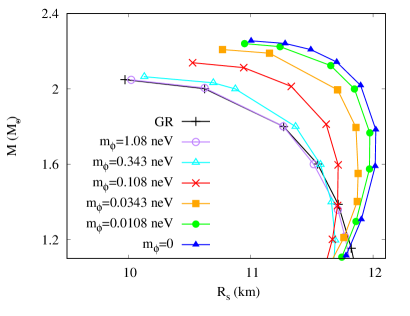
Figure 1: Mass $M$ in solar masses $M_{\odot}$ versus physical radius $R_{s}$ in km. The colors represent different values of the scalar field mass $m_{\phi}$, with the general relativistic limit in black.

Solutions describing neutron stars have to satisfy certain boundary conditions. At the center of the star, the configuration has to be regular. An expansion yields

$$\lambda=\left[\frac{4}{3}\pi A_{c}^{4}\hat{\rho}_{c}+\frac{1}{12}V_{c}\right]r^{2}+o(r^{4}),$$ (22)

$$\nu=\nu_{c}+\left[\frac{2}{3}\pi A_{c}^{4}(3\hat{p}_{c}+\hat{\rho}_{c})-\frac{1}{12}V_{c}\right]r^{2}+o(r^{4}),$$ (23)

$$\hat{p}=\hat{p}_{c}+(\hat{p}_{c}+\hat{\rho}_{c})\left[\frac{2\pi A_{c}^{3}}{3\sqrt{3}}\frac{dA_{0}}{d\phi_{0}}\biggr{\rvert}_{c}(3\hat{p}_{c}-\hat{\rho}_{c})+\frac{\sqrt{3}}{72}\frac{dV_{0}}{d\phi_{0}}\biggr{\rvert}_{c}+\left(\frac{V_{c}}{12}-\frac{2\pi}{3}A_{c}^{4}(3\hat{p}_{c}+\hat{\rho}_{c})\right)\right]r^{2}+o(r^{4}),$$ (24)

$$\phi_{0}=\phi_{c}+\left[\frac{2\pi}{3}A_{c}^{3}\frac{dA_{0}}{d\phi_{0}}\biggr{\rvert}_{c}(3\hat{p}_{c}-\hat{\rho}_{c})+\frac{1}{24}\frac{dV_{0}}{d\phi_{0}}\biggr{\rvert}_{c}\right]r^{2}+o(r^{4}),$$ (25)

where $\nu_{c}=\nu(0)$, $\hat{p}_{c}=\hat{p}(0)$, $\phi_{c}=\phi_{0}(0)$, $V_{c}=V_{0}(\phi_{c})$, $A_{c}=A_{0}(\phi_{c})$, etc. This expansion has only three free parameters $\nu_{c}$, $\hat{p}_{c}$ and $\phi_{c}$, the others being determined by the couplings and the equation of state. However, a global solution that is asymptotically flat will have only one free parameter at the center (typically chosen to be the central pressure $\hat{p_{c}}$ in the numerical calculations).

The border of the neutron star is defined by the point $r=r_{s}$, where the pressure vanishes, $\hat{p}_{0}(r_{s})=0$. The physical (Jordan frame) radius of the star is given by $R_{s}=A(\phi_{0}(r_{s}))r_{s}$, see (Blázquez-Salcedo et al., 2018) for more details. Outside the neutron star there is no fluid, thus $\hat{p}_{0}=\hat{\rho}_{0}=0$ in equations (18-21). We are interested in asymptotically flat solutions with vanishing scalar field at infinity. However, for ${a}\neq 0$, the scalar field outside the star does not vanish. Nonetheless, sufficiently far from the star, the scalar field decays exponentially with $\phi\sim\frac{1}{r}e^{-m_{\phi}r}$, and the background metric is essentially given by the Schwarzschild solution, with $e^{2\nu}=e^{-2\lambda}\sim 1-2M/r$, where $M$ is the total mass of the neutron star.

The mass–radius relation for most of the background neutron star configurations investigated in the following is exhibited in Figure 1, where the mass $M$ is given in solar masses $M_{\odot}$ and the physical (Jordan frame) radius $R_{s}$ in km. The chosen potential is $V_{II}$ ($R^{2}$ gravity), and the scalar field mass $m_{\phi}$ assumes several values in the physically interesting mass range (Naf and Jetzer, 2010; Brito et al., 2017). The color coding is purple, cyan, red, orange and green for $m_{\phi}=1.08$, $0.343$, $0.108$, $0.0343$ and $0.0108$ neV, respectively. Also shown are the general relativistic limit (black), and the case of a massless scalar field (blue). For the SLy equation of state the maximum mass of static neutron stars in General Relativity is slightly above two solar masses. In the STTs studied, the value of the maximum mass is increased the more, the smaller the scalar field mass is, reaching about 2.25 solar masses. At the same time, the neutron star radii become larger except for rather small neutron star masses.

4 Perturbations in massive scalar-tensor theory

4.1 Setup

In this section we present the quasinormal mode formalism, focusing on polar perturbations. In the Einstein frame, we perturb the background metric, the scalar field and the fluid in the following way:

$$g_{\mu\nu}=g_{\mu\nu}^{(0)}(r)+\epsilon h_{\mu\nu}(t,r,\theta,\varphi)~{},$$ (26)

$$\phi=\phi_{0}(r)+\epsilon\delta\phi(t,r,\theta,\varphi)~{},$$ (27)

$$\rho=\rho_{0}(r)+\epsilon\delta\rho(t,r,\theta,\varphi)~{},$$ (28)

$$p=p_{0}(r)+\epsilon\delta p(t,r,\theta,\varphi)~{},$$ (29)

$$u_{\mu}=u^{(0)}_{\mu}(r)+\epsilon\delta u_{\mu}(t,r,\theta,\varphi)~{},$$ (30)

where $\epsilon<<1$ is the perturbation parameter. The zeroth order of the configurations describes a static and spherically symmetric background, discussed in the previous section, while the perturbations are in general dependent on time, radial coordinate and angular directions.

Assuming that the perturbation functions can be expanded as a product of radial, temporal and angular components, they can be further separated into classes of axial and polar perturbations, depending on the transformation of the angular component under parity (Regge and Wheeler, 1957; Zerilli, 1970; Thorne and Campolattaro, 1967; Price and Thorne, 1969; Thorne, 1969; Campolattaro and Thorne, 1970; Thorne, 1980; Detweiler and Lindblom, 1985; Chandrasekhar and Ferrari, 1991; Chandrasekhar et al., 1991b, a; Ipser and Price, 1991; Kojima, 1992; Fernandez-Jambrina and Gonzalez-Romero, 2003). For polar perturbations, the spherical harmonics transform as $Y_{lm}(\theta,\varphi)\rightarrow Y_{lm}(\pi-\theta,\pi+\varphi)=(-1)^{l}Y_{lm}(\theta,\varphi)$. For a study of the current theory in the axial case we refer the reader to (Blázquez-Salcedo et al., 2018).

The Ansatz for the polar perturbations of the metric is

$$h_{\mu\nu}^{(\text{polar})}=\sum\limits_{l,m}\,\int\left[\begin{array}[]{c c c c}r^{l}e^{2\nu}H_{0}Y_{lm}&-i\omega r^{l+1}H_{1}Y_{lm}&0&0\\ -i\omega r^{l+1}H_{1}Y_{lm}&r^{l}e^{2\lambda}H_{2}Y_{lm}&0&0\\ 0&0&r^{l+2}KY_{lm}&0\\ 0&0&0&r^{l+2}\sin^{2}\theta KY_{lm}\\ \end{array}\right]e^{-i\omega t}d\omega~{},$$ (31)

in the order of $(t,r,\theta,\varphi)$ in the rows and columns of the matrix. The functions $H_{0},H_{1},H_{2},K$ only depend on the radial coordinate $r$, the integer multipole numbers $l$, $m$, and the complex wave frequency $\omega$, where $\omega=\omega_{R}+i\omega_{I}$ for $\omega_{R},\omega_{I}\in\mathbb{R}$. The functions $Y_{lm}$ are the standard spherical harmonics. The scalar field can be decomposed as

$$\delta\phi=\sum\limits_{l,m}\,\int r^{l}\phi_{1}\,Y_{lm}e^{-i\omega t}d\omega~{},$$ (32)

where again the function $\phi_{1}$ depends on $r,l,m$ and $\omega$.

Concerning the perturbation of the fluid inside the star, the scalar quantities, such as the energy density $\rho$ and pressure $p$, can be decomposed similarly to the scalar field

$$\delta\rho=\sum\limits_{l,m}\,\int r^{l}E_{1}Y_{lm}e^{-i\omega t}d\omega~{},\quad\delta p=\sum\limits_{l,m}\,\int r^{l}\Pi_{1}Y_{lm}e^{-i\omega t}d\omega~{},$$ (33)

while the perturbation of the 4-velocity is given by

$$\delta u_{\mu}=\sum\limits_{l,m}\,\int\left[\begin{array}[]{c}\frac{1}{2}r^{l}e^{\nu}H_{0}Y_{lm}\\ r^{l}i\omega e^{-\nu}\left(e^{\lambda}W/r-rH_{1}\right)Y_{lm}\\ -i\omega r^{l}e^{-\nu}V\partial_{\theta}Y_{lm}\\ -i\omega r^{l}e^{-\nu}V\partial_{\phi}Y_{lm}\\ \end{array}\right]e^{-i\omega t}d\omega~{},$$ (38)

The functions $V$ and $W$ depend on $r,l,m,\omega$.

Before continuing, we note that although we have given the perturbations in the Einstein frame, they can be alternatively defined in the Jordan frame. Perturbations in the Jordan frame for the scalar and the metric ($\delta\psi$ and $h_{\mu\nu}^{*}$, respectively) can be expressed as a combination of the perturbations in the Einstein frame,

$$\delta\psi=\frac{2}{\sqrt{3}}e^{\frac{2}{\sqrt{3}}\phi_{0}}\delta\phi~{},\quad h_{\mu\nu}^{*}=e^{-\frac{2}{\sqrt{3}}\phi_{0}}(h_{\mu\nu}-\frac{2}{\sqrt{3}}g_{\mu\nu}^{(0)}\delta\phi)~{}.$$ (39)

Concerning the energy density and pressure, the barotropic equation of state in the Jordan frame implies a relation between the perturbations $\delta p$, $\delta\rho$ and $\delta\phi$

$$\delta\rho=\frac{d\hat{\rho}_{0}}{d\hat{p}_{0}}\delta p+4A_{0}^{3}\frac{dA_{0}}{d\phi_{0}}(\hat{\rho}_{0}-\hat{p}_{0}\frac{d\hat{\rho}_{0}}{d\hat{p}_{0}})\delta\phi~{}.$$ (40)

4.2 Equations of the polar perturbations

Employing the Ansatz shown in the previous section for the perturbations on the field equations (12) and (16), leads to a system of ordinary differential equations in $r$, that is characterized by the eigenvalue $\omega$, and the multipole number $l$, but that is independent of $m$ because of the spherical symmetry.

The modified Einstein equation (12) result in six ordinary differential equations

$${\frac{{d}^{2}{K}}{{d}{r}^{2}}}=-8\pi{{e}^{2\lambda}}{E_{1}}+\frac{1}{2r^{2}}{{\left(2\left({\frac{d\phi_{0}}{{d}r}}\right)^{2}{r}^{2}-4r{\frac{d\lambda}{{d}r}}+({l}{{e}^{2\lambda}}+2)(l+1)\right){H_{2}}}}$$

$$+2{\frac{d\phi_{0}}{{d}r}}{\frac{d\phi_{1}}{{d}r}}+\frac{1}{6r}{{\left(\sqrt{3}e^{2\lambda}\frac{r}{a}({{e}^{-\frac{4}{\sqrt{3}}\phi_{0}}}-{{e}^{-\frac{2}{\sqrt{3}}\phi_{0}}})-12l{\frac{d\phi_{0}}{{d}r}}\right)\phi_{1}}}$$

$$+\frac{1}{2r^{2}}{{\left(2lr{\frac{d\lambda}{{d}r}}+{{e}^{2\lambda}}(l(l+1)-2)-2l(l+2)\right){K}}}+{\frac{\left(r{\frac{d\lambda}{{d}r}}-2l-3\right)}{r}}{\frac{d{K}}{{d}r}}+{\frac{1}{r}}{\frac{d{H_{2}}}{{d}r}}$$

$$+\frac{1}{8r^{2}}{{\left(64\pi\rho{r}^{2}{{e}^{2\lambda}}+8\left({\frac{d\phi_{0}}{{d}r}}\right)^{2}{r}^{2}+e^{2\lambda}\frac{{r}^{2}}{a}({{e}^{-\frac{2}{\sqrt{3}}\phi_{0}}}-1)^{2}-16r{\frac{d\lambda}{{d}r}}+8(1-e^{2\lambda})\right){H_{0}}}}~{},$$ (41)

$${\frac{d{K}}{{d}r}}={\frac{1}{r}}{H_{2}}+{\frac{\left({\frac{d\nu}{{d}r}}r-l-1\right)}{r}}{K}-2{\frac{d\phi_{0}}{{d}r}}\phi_{1}-8\pi{\frac{{{e}^{\lambda}}\left(p+\rho\right)}{r}}{W}$$

$$+\frac{1}{8r}{{\left(4l(l+1)-16{\frac{d\lambda}{{d}r}}r{{e}^{-2\lambda}}+8({{e}^{-2\lambda}}-1)\right){H_{1}}}}$$

$$+\frac{1}{8r}{{\left(64\pi\rho{r}^{2}-\frac{r^{2}}{a}({{e}^{-\frac{2}{\sqrt{3}}\phi_{0}}}-1)^{2}+8\left({\frac{d\phi_{0}}{{d}r}}\right)^{2}{r}^{2}{{e}^{-2\lambda}}\right){H_{1}}}}~{},$$ (42)

$${\frac{d{H_{1}}}{{d}r}}={\frac{{{e}^{2\lambda}}}{r}}{H_{2}}+{\left({\frac{d\lambda}{{d}r}}-{\frac{d\nu}{{d}r}}-\frac{l+1}{r}\right)}{H_{1}}+{\frac{{{e}^{2\lambda}}}{r}}{K}-\frac{16\pi}{r}{{{{e}^{2\lambda}}\left(p+\rho\right)}}{V}~{},$$ (43)

$${\frac{d{H_{0}}}{{d}r}}=-8\pi{{e}^{2\lambda}}r{\Pi_{1}}-2r{\omega}^{2}{{e}^{-2\nu}}{H_{1}}+\frac{l}{2r}{{\left((l+1){{e}^{2\lambda}}-2\right){H_{0}}}}-2r{\frac{d\phi_{0}}{{d}r}}{\frac{d\phi_{1}}{{d}r}}$$

$$-\frac{1}{8r}{{\left(64\pi{{e}^{2\lambda}}p{r}^{2}-\frac{r^{2}}{a}e^{2\lambda}({{e}^{-\frac{2}{\sqrt{3}}\phi_{0}}}-1)^{2}+8{{e}^{2\lambda}}\right){H_{2}}}}$$

$$+\frac{1}{2r}{{\left(2{{e}^{2(\lambda-\nu)}}{\omega}^{2}{r}^{2}-{{e}^{2\lambda}}(l-1)(l+2)+2l\left(r{\frac{d\nu}{{d}r}}+1\right)\right){K}}}$$

$$+\left(\frac{1}{2\sqrt{3}}\frac{r}{a}e^{2\lambda}({{e}^{-\frac{2}{\sqrt{3}}\phi_{0}}}-{{e}^{-\frac{4}{\sqrt{3}}\phi_{0}}})-2l{\frac{d\phi_{0}}{{d}r}}\right)\phi_{1}+\left(r{\frac{d\nu}{{d}r}}+1\right){\frac{d{K}}{dr}}~{},$$ (44)

$${\frac{dH_{0}}{{d}r}}=-{{\left({\frac{d\nu}{{d}r}}+\frac{1}{r}\right){H_{2}}}}-r{\omega}^{2}{{e}^{-2\nu}}{H_{1}}-{{\left({\frac{d\nu}{{d}r}}+\frac{l-1}{r}\right){H_{0}}}}+{\frac{l}{r}}{K}+4{\frac{d\phi_{0}}{{d}r}}\phi_{1}+{\frac{d{K}}{{d}r}}~{},$$ (45)

$${\frac{{d}^{2}{K}}{{d}{r}^{2}}}-{\frac{{d}^{2}{H_{0}}}{{d}{r}^{2}}}=16\pi{{e}^{2\lambda}}{\Pi_{1}}-4\left({\frac{d\phi_{0}}{{d}r}}\right){\frac{d\phi_{1}}{{d}r}}+\left({\frac{d\nu}{{d}r}}+\frac{1}{r}\right){\frac{d{H_{2}}}{{d}r}}+2r{\omega}^{2}{{e}^{-2\nu}}{\frac{d{H_{1}}}{{d}r}}$$

$$-2{{e}^{-2\nu}}{\omega}^{2}\left(r{\frac{d\lambda}{{d}r}}-l-2\right){H_{1}}-\frac{1}{2{{r}^{2}}}{l\left(2r{\frac{d\lambda}{{d}r}}-4r{\frac{d\nu}{{d}r}}+l{{e}^{2\lambda}}+{{e}^{2\lambda}}-2l\right){H_{0}}}$$

$$+\frac{1}{2{{r}^{2}}}{\left(-2{{e}^{-2\nu+2\lambda}}{\omega}^{2}{r}^{2}+4\left({\frac{d\phi_{0}}{{d}r}}\right)^{2}{r}^{2}-4{r}^{2}{\frac{d\lambda}{{d}r}}{\frac{d\nu}{{d}r}}+4\left({\frac{d\nu}{{d}r}}\right)^{2}{r}^{2}+4{r}^{2}{\frac{{d}^{2}\nu}{{d}{r}^{2}}}\right){H_{2}}}$$

$$+\frac{1}{2{{r}^{2}}}{\left(+{l}^{2}{{e}^{2\lambda}}+2lr{\frac{d\nu}{{d}r}}-4r{\frac{d\lambda}{{d}r}}+l{{e}^{2\lambda}}+4r{\frac{d\nu}{{d}r}}+2l\right){H_{2}}}$$

$$+\frac{1}{4r^{2}}{\left(64\pi{{e}^{2\lambda}}p{r}^{2}-4{{e}^{-2\nu+2\lambda}}{\omega}^{2}{r}^{2}+8{r}^{2}{\frac{d\lambda}{{d}r}}{\frac{d\nu}{{d}r}}-8\left({\frac{d\phi_{0}}{{d}r}}\right)^{2}{r}^{2}-8\left({\frac{d\nu}{{d}r}}\right)^{2}{r}^{2}\right){K}}$$

$$+\frac{1}{4r^{2}}{\left(4r(l+2)\left({\frac{d\lambda}{{d}r}}-{\frac{d\nu}{{d}r}}\right)-8{r}^{2}{\frac{{d}^{2}\nu}{{d}{r}^{2}}}-4l(l+1)-\frac{{r}^{2}}{a}e^{2\lambda}(1-{{e}^{-\frac{2}{\sqrt{3}}\phi_{0}}})^{2}\right){K}}$$

$$+\frac{1}{3{r}}{{\left(\sqrt{3}\frac{r}{a}e^{2\lambda}\left({{e}^{-\frac{4}{\sqrt{3}}\phi_{0}}}-{{e}^{-\frac{2}{\sqrt{3}}\phi_{0}}}\right)-12l{\frac{d\phi_{0}}{{d}r}}\right)\phi_{1}}}$$

$$+\left(\frac{1}{r}(2l+1)-{\frac{d\lambda}{{d}r}}+2{\frac{d\nu}{{d}r}}\right){\frac{d{H_{0}}}{{d}r}}+\left({\frac{d\lambda}{{d}r}}-{\frac{d\nu}{{d}r}}-{\frac{2}{r}}(l+1)\right){\frac{d{K}}{{d}r}}~{}.$$ (46)

In addition, it imposes the constraint

$$H_{2}=H_{0}~{}.$$ (47)

The scalar field equation (16) results in

$${\frac{{d}^{2}\phi_{1}}{{d}{r}^{2}}}=-\frac{4}{\sqrt{3}}\pi{{e}^{2\lambda}}{(E_{1}-3\Pi_{1})}+{\frac{l}{2r}}{\frac{d\phi_{0}}{{d}r}}{H_{0}}+{\frac{d\phi_{0}}{{d}r}}{{e}^{-2\nu}}{\omega}^{2}r{H_{1}}-{\frac{l}{r}}{\frac{d\phi_{0}}{{d}r}}K$$

$$+\frac{1}{6r^{2}}{{\left(-e^{2\lambda}r^{2}\left(6{{e}^{-2\nu}}{\omega}^{2}+({{e}^{-\frac{2}{\sqrt{3}}\phi_{0}}}-2{{e}^{-\frac{4}{\sqrt{3}}\phi_{0}}})\frac{1}{a}\right)+6lr\left({\frac{d\lambda}{{d}r}}-{\frac{d\nu}{{d}r}}\right)+6l(1+l)({{e}^{2\lambda}}-1)\right)\phi_{1}}}$$

$$+\frac{1}{2r}{{\left(-2r{\frac{d\phi_{0}}{{d}r}}{\frac{d\lambda}{{d}r}}+2r{\frac{d\phi_{0}}{{d}r}}{\frac{d\nu}{{d}r}}+2r{\frac{{d}^{2}\phi_{0}}{{d}{r}^{2}}}+{\frac{d\phi_{0}}{{d}r}}l+4{\frac{d\phi_{0}}{{d}r}}\right){H_{2}}}}$$

$$+{{\left({\frac{d\lambda}{{d}r}}-{\frac{d\nu}{{d}r}}-\frac{2}{r}(l+1)\right)}}{\frac{d\phi_{1}}{{d}r}}+\frac{1}{2}{\frac{d\phi_{0}}{{d}r}}\left({\frac{d{H_{2}}}{{d}r}}+{\frac{d{H_{0}}}{{d}r}}-2{\frac{d{K}}{{d}r}}\right)~{}.$$ (48)

The barotropic condition on the equation of state (40) becomes a relation between the energy density perturbation, pressure perturbation and scalar field perturbation,

$${E_{1}}=\frac{d\hat{\rho}_{0}}{d\hat{p}_{0}}{\Pi_{1}}-\frac{4}{\sqrt{3}}{{\rm e}^{-\frac{4}{\sqrt{3}}\phi_{0}}}\left(\hat{\rho}_{0}-\hat{p}_{0}\frac{d\hat{\rho}_{0}}{d\hat{p}_{0}}\right)\phi_{1}~{}.$$ (49)

By tedious algebraic manipulations the nine equations (4.2)-(49) can be simplified. For this purpose it is convenient to define the following function of the perturbations (Lindblom and Detweiler, 1983),

$$X={\omega}^{2}\left(\hat{p}_{0}+\hat{\rho}_{0}\right){{e}^{-\nu}}{V}-\frac{1}{r}{\frac{d\hat{p}_{0}}{{d}r}}{{e}^{\nu-\lambda}}{W}+\frac{1}{2}\left(\hat{p}_{0}+\hat{\rho}_{0}\right){{e}^{\nu}}{H_{0}}~{}.$$ (50)

The resulting minimal system of differential equations is given by a set of six first order differential equations for the functions $\Psi=(K,H_{1},W,X,\phi_{1},\frac{d\phi_{1}}{dr})$, which takes the form

$$\frac{d}{dr}\Psi+\sigma\Psi=0~{},$$ (51)

where $\sigma$ is a matrix that depends in a complicated way on the static functions $\nu,\lambda,\phi_{0},\hat{p}_{0},\hat{\rho}_{0}$, and also on the eigenvalue $\omega$ and the multipole number $l$.

Note that inside the star, the perturbation is described by the functions $(K,H_{1})$, which parametrize the metric perturbation, $(W,X)$ which parametrize the fluid perturbation and $(\phi_{1},\frac{d\phi_{1}}{dr})$ which is the scalar field perturbation. Outside the star, the system simplifies, since $\hat{p}=\hat{\rho}=0$. For instance, $W=X=0$ when there is no fluid, and the system reduces to a system of four first order differential equations for $(K,H_{1})$ (metric) and $(\phi_{1},\frac{d\phi_{1}}{dr})$ (scalar field).

Let us note that in STTs all perturbation equations are coupled with each other, whereas in the general relativistic limit, the system decouples on one hand into the metric and fluid perturbations, and on the other hand into the scalar field perturbation, which is simply governed by the minimally coupled scalar test field equation in the general relativistic limit.

4.3 Boundary conditions and asymptotic behaviour

At the center of the star we impose regularity of the perturbations. This means that at the center of the star the perturbation functions satisfy the constraints

$$l(l+1)H_{1}(0)-2lK(0)-16\pi A_{c}^{4}(\hat{p}_{c}+\hat{\rho}_{c})W(0)=0,$$

$$l\Pi_{1}(0)+\frac{l}{\sqrt{3}}A_{c}^{4}(3\hat{p}_{c}-\hat{\rho}_{c})\phi_{1}(0)+A_{c}^{4}(\hat{p}_{c}+\hat{\rho}_{c})\left(\frac{l}{2}K(0)-\omega^{2}e^{-2\nu_{c}}W(0)\right)=0,$$

$$\frac{le^{-\nu_{c}}}{\hat{p}_{c}+\hat{\rho}_{c}}X(0)-\frac{l}{2}K(0)=\left(\frac{8\pi l}{9}A_{c}^{4}(3\hat{p}_{c}+2\hat{\rho}_{c})-e^{-2\nu_{c}}\omega^{2}-\frac{l}{72a}(e^{-\frac{4}{\sqrt{3}}\phi_{c}}-4e^{-\frac{2}{\sqrt{3}}\phi_{c}}+3)\right)W(0),$$

$$\frac{d\phi_{1}}{dr}(0)=0\,,\,\,\,lV(0)+W(0)=0\,,\,\,\,H_{2}(0)-K(0)=0\,,\,\,\,H_{0}(0)-K(0)=0.$$ (52)

At infinity the massive scalar field is exponentially suppressed. Therefore the scalar perturbation is effectively asymptotically decoupled from the metric perturbations. Consequently, sufficiently far from the star, the oscillation can be described by the standard Zerilli function $Z_{g}(r)$ given by

$$H_{1}(r)=\frac{3M(nr+M)-nr^{2}}{r^{l+1}(2M-r)(nr+3M)}Z_{g}(r)+\frac{r}{r^{l}(r-2M)}F_{g}(r),$$ (53)

$$K(r)=\frac{nr^{2}(n+1)+3M(nr+2M)}{r^{l+2}(nr+3M)}Z_{g}(r)+\frac{1}{r^{l}}F_{g}(r),$$ (54)

where $n=l(l+1)/2$, and $F_{g}(r)$ is some supplementary function. Then the two first order equations for $(K,H_{1})$ can be rewritten as a more standard Schrödinger-like equation for $Z_{g}$

$$\frac{d^{2}Z_{g}}{dy^{2}}=(G_{g}(r)-\omega^{2})Z_{g}$$ (55)

with tortoise coordinate $\frac{dy}{dr}=e^{\lambda-\nu}$ and the effective potential $G_{g}(r)$ for space-time perturbations

$$G_{g}(r)=\frac{2(r-2M)}{r^{4}(nr+3M)^{2}}\left(n^{2}(n+1)r^{3}+3Mn^{2}r^{2}+9M^{2}nr+9M^{3}\right)~{}.$$ (56)

Note that asymptotically, the potential goes to zero, $G_{g}(r\to\infty)\to 0$. Therefore the asymptotic behaviour of the perturbation is given by the combination of an ingoing and an outgoing solution of the form

$$Z_{g}\sim A_{in}e^{-i\omega y}+A_{out}e^{i\omega y}\ .$$ (57)

We now consider the scalar field. Since this component decouples exponentially from the metric perturbation sufficiently far from the star, the scalar field equation can also be reformulated as a Schrödinger-like equation. Defining

$$\phi_{1}(r)=r^{l}Z_{s}(r)~{},$$ (58)

the equation then becomes

$$\frac{d^{2}Z_{s}}{dy^{2}}=(G_{s}(r)-\omega^{2})Z_{s}\$$ (59)

with the (same) tortoise coordinate $y$, and $G_{s}(r)$ denotes the effective potential for scalar perturbations

$$G_{s}(r)=\left(1-\frac{2M}{r}\right)\left(\frac{1}{r^{2}}\left(l(l+1)+\frac{2M}{r}\right)+\frac{1}{6a}\right)~{}.$$ (60)

Note that in this case, the potential goes asymptotically to $G_{s}(r\to\infty)\to\frac{1}{6a}=m_{\phi}^{2}$. Therefore the scalar perturbation is asymptotically also given by a combination of outgoing and ingoing waves, but now of the form

$$Z_{s}\sim A_{in}e^{-i\Omega y}+A_{out}e^{i\Omega y}\ ,$$ (61)

where $\Omega$ satisfies the following dispersion relation for the scalar field perturbations

$$\Omega^{2}=\omega^{2}-m_{\phi}^{2}\ .$$ (62)

The appearance of $\Omega$ is related to the fact that the scalar field perturbations cannot propagate at the speed of light, like the space-time perturbations, since for finite values of $a$, the scalar field is massive. Only in the limit of $a\to\infty$ the scalar field becomes massless and we recover $\Omega=\omega$.

4.4 Outline of the numerical method

We now briefly summarize the numerical implementation of the quasinormal mode calculations. The very first step is the calculation of the background configurations. To this end we solve the static equations using Colsys (Ascher et al., 1979). The solutions are obtained by employing a compactified coordinate $x=\frac{r}{r_{s}+r}$, which allows to impose the physical boundary conditions exactly at the center of the star, at its surface $r_{s}$ and at infinity. The input parameters are the central pressure $\hat{p}_{c}$ and the scalar field mass $m_{\phi}$. The system has to be complemented with an equation of state. In this paper we shall focus on one particular choice for the equation of state, the SLy EOS (Douchin and Haensel, 2001), which is a representative model that captures the basic features of realistic neutron star models. We implement this equation of state by using a piece-wise polytropic approximation (Read et al., 2009).

Once a particular background star with mass $M$ is calculated, it is used to calculate the coefficients of the matrix $\sigma$ of equation (51). Then we proceed to calculate the quasinormal modes for a particular configuration and a particular multipole number $l$. To do so, we solve the perturbation equations for a fixed value of $\omega$ in three different steps.

First we obtain two independent solutions of equation (51) inside the star, satisfying the conditions (4.3), and imposing $X(r_{s})=0$. Second, these two solutions are continued outside the star, by requiring continuity of the metric and scalar field perturbations. These solutions are obtained up to some point $r_{i}>r_{s}$. We choose this $r_{i}$ so that $\phi_{0}(r_{i})\lesssim 10^{-4}$. In the third step, we calculate the phases of the metric and scalar perturbations in the background of a Schwarzschild solution with mass $M$. We impose purely outgoing wave solutions at infinity for both phases. To do so, we make use of the exterior complex scaling method on equations (55) and (59). For more details we refer the reader to (Blázquez-Salcedo et al., 2013, 2014, 2016a; Blázquez-Salcedo and Eickhoff, 2018; Altaha Motahar et al., 2018, 2019; Blázquez-Salcedo et al., 2018, 2019).

Then we check if the phases obtained for the asymptotic behaviour of the perturbation, which satisfy the outgoing wave behaviour, match with the full perturbative solution obtained in a region $0<r<r_{i}$. If they match, then $\omega$ is the eigenvalue of a quasinormal mode. If not, we repeat the process for different values of $\omega$ until matching is achieved. In this way, we investigate the spectrum for numerous configurations for several values of the scalar field mass $m_{\phi}$.

5 Results

Because of the nature of the polar perturbations, the spectrum of polar perturbations is much richer than the spectrum of axial perturbations, which involve only spacetime perturbations. Polar modes on the contrary feature different families of modes. In General Relativity static and spherically symmetric neutron stars not only possess spacetime modes (w-modes), they also possess modes related to the fluid perturbation. For $l\geq 2$, the spectrum is dominated by the fundamental mode (f-mode), a nodeless fluctuation driven by pressure oscillations inside the star, which typically possesses the lowest frequency. But there are also excited pressure modes (p-modes) with higher values of the frequency.

When considering radial perturbations in General Relativity, stars are seen to possess a family of normal modes with $\omega^{2}\in\mathbb{R}$, that become unstable beyond the maximum mass of the equation of state. These modes are well known in the literature (Chandrasekhar, 1964a, a; Bardeen et al., 1966; Meltzer and Thorne, 1966; Chanmugam, 1977; Glass and Lindblom, 1983; Vaeth and Chanmugam, 1992; Datta et al., 1998). However, in General Relativity radial perturbations cannot propagate gravitational radiation outside the neutron star.

In STTs there is another degree of freedom, the scalar field $\phi$. Therefore similarly to the scalar modes of hairy black holes (Blázquez-Salcedo et al., 2016b, 2017, 2019), there are additional modes for scalarized neutron stars. The $l=0$ modes can propagate outside the neutron stars in STTs, which makes them relevant for the study of gravitational waves. In addition, of course, dipole ($l=1$) modes arise. These and the $l=0$ modes are supported by the scalar field, but they are coupled via the field equations with oscillations of the metric and the neutron star fluid.

5.1 Quadrupole modes

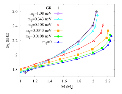
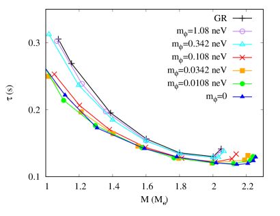
Figure 2: Frequency $\omega_{R}$ in kHz (left) and damping time $\tau$ in s (right) versus the total mass of the neutron star $M$ ($M_{\odot}$) for the $l=2$ f-mode. The colors represent different values of the scalar field mass $m_{\phi}$, with the general relativistic limit in black.

We start our discussion of the results with a detailed analysis of the properties of the quadrupole f-mode. The $l=2$ fundamental mode is probably the most interesting mode as regards to astrophysical scenarios, since simulations in General Relativity show, that it tends to dominate the ringdown spectrum after a merger.

In Figure 2 we show the $l=2$ fundamental mode for several values of the scalar field mass $m_{\phi}$. In the left panel we show the frequency as a function of the total mass (in units of solar masses), and in the right panel the damping time (in seconds) as a function of the total mass. Different colors symbolize different values of the parameter $a$, and thus the scalar field mass $m_{\phi}$, with purple, cyan, red, orange and green for $m_{\phi}=1.08$, $0.343$, $0.108$, $0.0343$ and $0.0108$ neV, respectively. In blue we show the massless case, and in black the general relativistic values for comparison. Note that for $1.08$ neV the values are already very close to those of General Relativity, while below $m_{\phi}=1$ peV the values do not deviate significantly from the blue curve. The range of masses considered, $0.0108\leq m_{\phi}\leq 1.08$ neV, is compatible with current observations and constraints on the mass of a hypothetical ultra light boson (Naf and Jetzer, 2010; Brito et al., 2017).

Overall we observe that the frequency and the damping time do not change drastically when going to these STTs, finding typical variations within $10\%$ of the general relativistic value. This behaviour is reminiscent of the previous observations for the axial modes (Blázquez-Salcedo et al., 2018). Figure 2 (left) shows that a decrease of the mass of the scalar field leads to a decrease of the frequency, except for values of the stellar mass close to one solar mass, where the frequency rises slightly from the general relativistic value. Regarding the damping time, Figure 2 (right) shows that the overall value of $\tau$ decreases the more, the lighter the scalar field is.

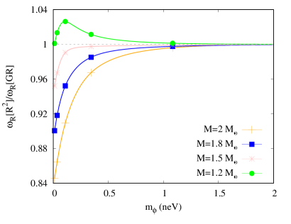
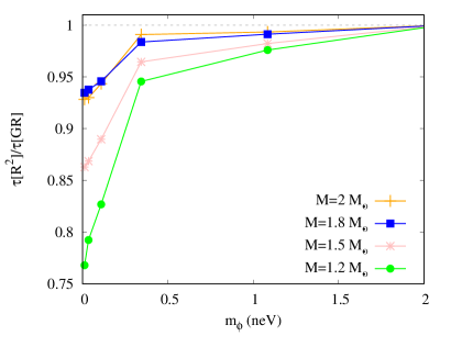
Figure 3: Frequency $\omega_{R}$ in kHz (left) and damping time $\tau$ in s (right) versus the mass of the scalar field $m_{\phi}$ in neV for the $l=2$ f-mode. The colors represent different values of the total mass $M$ of the star. The frequency is normalized in terms of the corresponding frequency for a star of given mass in General Relativity. This value is obtained asymptotically as the mass of the scalar field is increased.

To better understand the dependence of the fundamental mode on the mass $m_{\phi}$ of the scalar field, we now fix the mass $M$ of the star, while we vary $m_{\phi}$. In Figure 3 we show the $l=2$ fundamental mode as a function of the scalar field mass $m_{\phi}$. Each curve corresponds to a family of stars with fixed value of the mass, with orange, blue, pink and green for $M=2$, $1.8$, $1.5$, and $1.2M_{\odot}$, respectively. On the left we show the frequency and on the right the damping time, both normalized to the respective value in General Relativity. The figure clearly shows that the larger the scalar mass, the closer the frequency comes to the general relativistic value. In fact, the frequency and the damping time deviate only significantly when the scalar field mass is below the neV. The shortest damping time occurs for massless scalar fields, and the largest deviation occurs for not very massive neutron stars with $M=1.2M_{\odot}$. We note that for $M=1.2M_{\odot}$, the frequency rises slightly as the scalar mass is decreased. However, in general for sufficiently massive neutron stars, the maximum deviation of the frequency appears also for massless scalar fields, with a reduction of the frequency of around $10\%$.

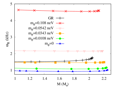
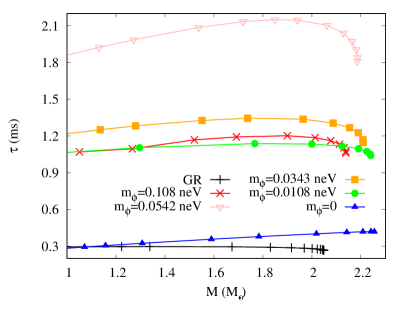
Figure 4: Frequency $\omega_{R}$ in kHz (left) and damping time $\tau$ in ms (right) versus the total mass of the neutron star $M$ ($M_{\odot}$) for the $l=2$ $\phi$-mode. The colors represent different values of the scalar field mass $m_{\phi}$, with the general relativistic limit in black.

The presence of the scalar field allows for an additional type of $l=2$ mode. In General Relativity this mode would correspond to the mode of an independent minimally coupled scalar field in the background of the neutron star, and therefore not be of much interest. In STTs, however, the equations for the scalar field perturbation and the matter and metric perturbations are coupled for polar modes. Therefore this new type of mode is necessarily present, and is dubbed $l=2$ $\phi$-mode, distinguishing it from the previously discussed $l=2$ f-mode.

In Figure 4 we show the $l=2$ $\phi$-mode as a function of the mass $M$ of the neutron star for several values of the scalar field mass $m_{\phi}$ as well as for General Relativity. Interestingly, there is very little dependence of the frequency and the damping time on the neutron star mass. Moreover, for most of the relevant mass range of the scalar field in these STTs the frequencies of these $\phi$-modes are lower than the frequencies of the corresponding f-modes. In contrast, the damping times of the $\phi$-modes (of the order ms) are much shorter than the damping times of the corresponding f-modes. In a ringdown spectrum the $\phi$-modes will therefore fast decay, leaving the f-modes to dominate the spectrum.

Let us also mention here that, although we have not made a systematic study of the $l=2$ excited modes, they also exist in the STTs. Our numerical results indicate that the overtones for both the f-mode and the $\phi$-mode always possess larger frequencies and shorter damping times than the corresponding ground states.

5.2 Radial modes

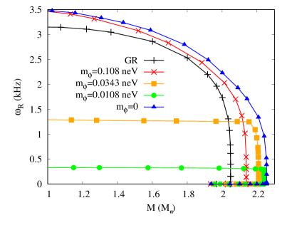
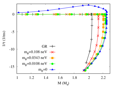
Figure 5: Frequency $\omega_{R}$ in kHz (left) and inverse instability timescale $\omega_{I}=1/\tau$ in 1/ms (right) versus the total mass of the neutron star $M$ ($M_{\odot}$) for the $l=0$ F-mode. The colors represent different values of the scalar field mass $m_{\phi}$, with the general relativistic limit in black.

Gravitational monopole radiation does not exist in GR. Hence, the ringdown phase in astrophysically realistic scenarios is expected to be dominated by the $l=2$ modes. In neutron stars the dominant mode would be the f-mode, discussed above. However, the additional scalar degree of freedom present in STTs implies that, in astrophysical scenarios, apart from the $l=2$ f-mode, also the radial $l=0$ modes could play an important role, when the neutron stars carry scalar hair.

The analysis of the $l=0$ modes in STTs reveals indeed a rich spectrum, consisting of two families of modes, named again according to their general relativistic limits. First, there are the modes that reduce to the oscillations of the nuclear matter in the general relativistic limit. These are the fundamental pressure-led mode, the F-mode, and its excitations, the H₁-mode, the H₂-mode, etc. Second, there are the modes that reduce to oscillations of an independent minimally coupled scalar field in the general relativistic limit. These are the $l=0$ $\phi$-modes.

As discussed above, in General Relativity the equations for these two types of modes are completely decoupled. The physically interesting modes in General Relativity are the pressure-led modes. They represent normal modes, since $l=0$ modes are confined to the interior of the stars here. The fundamental pressure-led mode, the F-mode, is of particular relevance, since it shows, that neutron stars become radially unstable beyond their maximum mass.

For the F mode the eigenvalue $\omega$ is a positive real number, as long as the mass $M$ of the neutron star increases with increasing central pressure, and the star is radially stable. Then $\omega$ becomes zero as the maximal neutron star mass is reached. Thus here a zero mode is encountered where the star is only marginally stable. Beyond the maximum mass of the star, $\omega$ becomes purely imaginary with $\omega_{I}$ negative, i.e., the star becomes radially unstable.

The $\phi$-modes, on the other hand, could in principle propagate outside the star, in case some external scalar field were minimally coupled to General Relativity, and a quasinormal mode analysis does yield a spectrum of such damped radial modes. However, the motivation for the presence of such a field in the environment of a neutron star would be typically lacking.

In STTs the picture changes almost completely. Only the instability of the stars beyond the maximum mass is still revealed by a purely imaginary eigenvalue with negative $\omega_{I}$. Most importantly, however, scalar radiation is a natural effect in STTs, since the scalar field is a relevant gravitational degree of freedom, that is intimately coupled with the tensor degrees of freedom. Consequently, the stable normal modes from General Relativity now turn into propagating and thus quasinormal modes (see e.g., the toy model studied in (Kokkotas and Schutz, 1986)): the presence of the gravitational scalar field now allows for these $l=0$ modes to propagate outside the star.

We exhibit in Fig. 5 the frequency $\omega_{R}$ in kHz (left) and the imaginary part $\omega_{I}$ in 1/ms (right) for the F-mode versus the total mass $M$ in solar masses $M_{\odot}$ for the neutron stars. As before, the colors represent different values of the scalar field mass $m_{\phi}$, and the general relativistic limit is shown in black. On the unstable neutron star branches beyond the maximum mass $\omega_{I}=1/\tau$ represents the inverse instability timescale.

On the stable neutron star branches, in contrast, the very small positive values of $\omega_{I}$ indicate the inverse damping time. While numerical inaccuracy does not allow us to precisely extract these values, the calculations indicate that the damping time is on the order of $\sim 10^{5}$ years or larger. This means that these F-modes are ultra long lived (Blázquez-Salcedo et al., 2020). In fact, these modes exist up to $m_{\phi}\to\infty$, where they turn into the normal modes of the respective general relativistic stars. Interestingly, long lived scalar radiation was also detected in core collapse processes in massive STTs (Sperhake et al., 2017; Rosca-Mead et al., 2020b; Rosca-Mead, 2020; Rosca-Mead et al., 2020a).

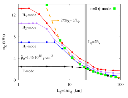
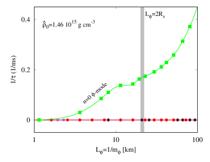
Figure 6: Frequency $\omega_{R}$ in kHz (left) and inverse damping time $\omega_{I}=1/\tau$ in 1/ms (right) versus the Compton wavelength $L_{\phi}=1/m_{\phi}$ in km for the $l=0$ F-, H₁-, H₂- and H₃-modes at fixed central density $\hat{{\rho}}_{0}$. For comparison, the inverse of the Compton wavelength $L_{\phi}$ is shown in orange (left) and the size of the neutron star $L_{\phi}=2R_{s}$ in grey.

In Figure 6 we show the frequency $\omega_{R}$ in kHz (left) and the inverse damping time $\omega_{I}=1/\tau$ in 1/ms (right) versus the Compton wavelength $L_{\phi}=1/m_{\phi}$ in km for the F-mode and the excited H-modes, H₁ – H₃, for a fixed value of the central density on the stable neutron star branch.

We note, that also for the excited modes the spectrum is qualitatively similar to the GR case. But again the fundamental difference is that the normal modes of General Relativity turn into quasinormal modes in the STTs, that are allowed to propagate outside the star, since the pressure-led modes induce also oscillations in the scalar field, which itself is coupled to the metric functions in the field equations. Moreover, the excited H-modes are ultra long lived, as well. As an aside we note, that in STTs with spontaneously scalarized neutron stars, analogous ultra long lived quasinormal modes have not been observed (Mendes and Ortiz, 2018).

For comparison Figure 6 (left) also shows the frequency which simply corresponds to the inverse of the Compton wavelength of the scalar field,

$$2\pi\omega_{R}=c/L_{\phi},$$ (63)

and the size of the neutron star

$$L_{\phi}=2R_{s},$$ (64)

where $R_{s}$ represents the radius of the family of stars. The figure shows, that for small values of the Compton wavelength $L_{\phi}$ the frequencies $\omega_{R}$ of the F-mode and the excited H-modes assume almost constant values, that increase with increasing excitation.

The (almost) $m_{\phi}$-independence ends for the fundamental F-mode when $L_{\phi}$ reaches the size of the star, and, analogously, for the excited H-modes, when appropriate fractions of the size of the star are reached. For the F-mode this happens when the Compton wavelength reaches $L_{\phi}=2R_{s}$ with $m_{\phi}=0.052$ neV, and for the first three H-modes for $m_{\phi}=0.072,0.16,0.19$ neV, respectively. For larger values of the Compton wavelength $L_{\phi}$ the frequencies decrease according to $\omega_{R}=1/2\pi L_{\phi}$, thus the frequencies simply follow the scale given by the mass of the scalar field, as depicted by the orange curve in the left figure.

Figure 6 (right) shows that the inverse decay times $1/\tau$ of the excited modes are indeed also very small. When estimating numerically the damping distances for these modes one finds that they should be equal or larger than $\sim 10^{5}$ ly. This corresponds to the size of a large galaxy like the Milky Way, and possibly even larger.

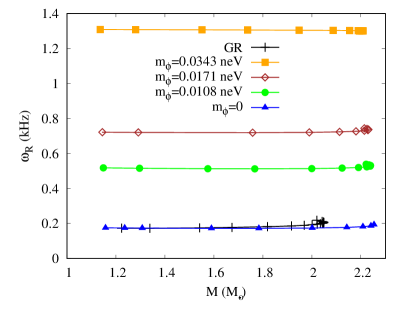
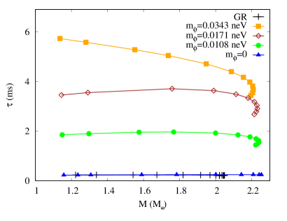
Figure 7: Frequency $\omega_{R}$ in kHz (left) and damping time $\tau$ in ms (right) versus the total mass of the neutron star $M$ ($M_{\odot}$) for the $l=0$ $\phi$-mode. The colors represent different values of the scalar field mass $m_{\phi}$, with the general relativistic limit in black.

As discussed above, in addition to the pressure-led $l=0$ modes there are also the scalar-led $l=0$ modes, the $\phi$-modes. Figure 6 also shows the fundamental $l=0$ $\phi$-mode. Its frequency $\omega_{R}$ follows always the scalar mass $m_{\phi}$, as seen by the overlap of the green dots ($\phi$-mode) and the orange curve (left). However, its imaginary part $\omega_{I}=1/\tau$ increases rapidly with increasing Compton wavelength $L_{\phi}$, showing that these modes possess much shorter lifetimes.

In Figure 7 we exhibit the frequency $\omega_{R}$ (kHz) (left) and the damping time $\tau$ (ms) (right) versus the total mass of the neutron star $M$ ($M_{\odot}$) for the $l=0$ $\phi$-mode. As already seen for the $l=2$ $\phi$-mode, the frequency $\omega_{R}$ changes only very little with the neutron star mass. The damping time shows so little dependence only in the limiting case of General Relativity, and for the massless scalar field.

As a comment, let us note here that scalar-led $l=0$ modes appear also in simulations of oscillating and collapsing neutron stars in chamaleon theories, in addition to the fluid modes (Dima et al., 2021).

5.3 Comparison of potentials

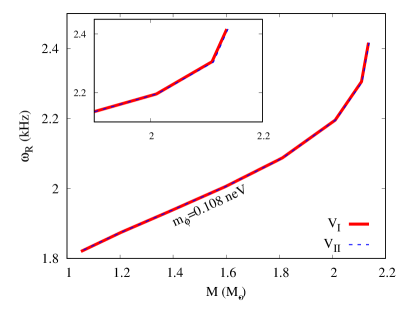
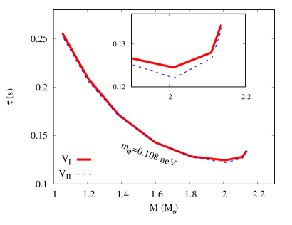
Figure 8: Frequency $\omega_{R}$ in kHz (left) and damping time $\tau$ in s (right) versus the total mass of the neutron star $M$ ($M_{\odot}$) for the $l=2$ f-mode. The colors represent the two potentials $V_{I}$ and $V_{II}$.

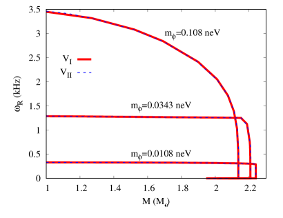
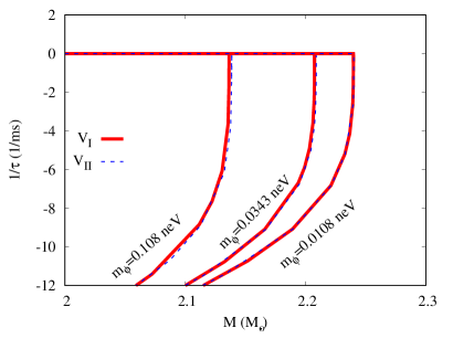
Figure 9: Frequency $\omega_{R}$ in kHz (left) and inverse instability timescale $\omega_{I}=1/\tau$ in 1/ms (right) versus the total mass of the neutron star $M$ ($M_{\odot}$) for the $l=0$ F-mode. The colors represent the two potentials $V_{I}$ and $V_{II}$.

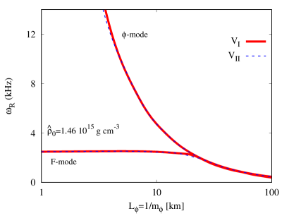
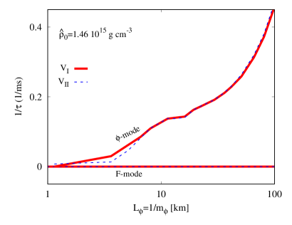
Figure 10: Frequency $\omega_{R}$ in kHz (left) and and inverse damping time $\omega_{I}=1/\tau$ in 1/ms (right) versus the Compton wavelength $L_{\phi}=1/m_{\phi}$ in km for the $l=0$ F-mode and $l=0$ $\phi$-mode at fixed central density $\hat{\rho}_{0}$. The colors represent the two potentials $V_{I}$ and $V_{II}$.

We finally briefly address the effect of the two different potentials, $V_{I}$ and $V_{II}$ (see Eqs. (4)), recalling that $V_{I}$ represents a STT with a mass term only, whereas $V_{II}$ is the potential derived from $R^{2}$ gravity. In Figure 8 we exhibit a comparison of the $l=2$ f-mode for both potentials and scalar mass $m_{\phi}=0.108$ neV. The insets highlight the differences.

In Figures 9 and 10 we exhibit a comparison of the radial modes. Figure 9 shows the $l=0$ F-mode versus the neutron star mass for several values of the scalar field mass. Figure 10 shows the $l=0$ F-mode and the $l=0$ $\phi$-mode versus the Compton wavelength of the scalar field for fixed central density.

From the figures we conclude, that for the range of masses $m_{\phi}$ of the scalar field that are of interest (Naf and Jetzer, 2010; Brito et al., 2017), i.e., $10^{-9}\gtrsim m_{\phi}\gtrsim 10^{-13}$ eV, there is very little deviation between the quasinormal modes in these two theories. Deviations are most noticeable for the most compact configurations, close to the maximum mass, and in particular in the damping times.

6 Conclusions

In this paper we have studied polar quasinormal modes of neutron stars in two STTs, one possessing a simple scalar field mass term and one corresponding to $R^{2}$ gravity. We have presented the set of equations and the boundary conditions necessary to obtain these modes. The scalar field mass $m_{\phi}$ leads to a dispersion relation between the frequency of the spacetime oscillations and the scalar field oscillations as infinity is asymptotically approached.

We have analyzed the quasinormal modes for the SLy equation of state, a realistic equation of state that yields for static neutron stars in General Relativity a maximum mass slightly above two solar masses. In the STTs studied, the value of the neutron star maximum mass increases with decreasing scalar field mass, reaching about 2.25 solar masses. For the scalar field we have covered, in particular, the physically interesting mass range (Naf and Jetzer, 2010; Brito et al., 2017).

We have investigated the $l=2$ modes, starting with the fundamental f-mode, and studied the effect of the mass of the gravitational scalar field of the STTs. Moreover, we have studied the $l=2$ $\phi$-modes, which represent a set of additional quadrupole radiation modes, present only in STTs. While they depend strongly on the scalar field mass, they depend only weakly on the neutron star mass.

In General Relativity, the quadrupole quasinormal modes represent the lowest multipole modes, that can propagate gravitational radiation. In STTs there is, of course, additional gravitational radiation, corresponding to $l<2$ modes. Here we have analyzed the $l=0$ quasinormal modes present in these STTs. In fact, the radial perturbations lead to a rich spectrum of modes.

We have shown that the pressure normal modes of General Relativity, the fundamental F-mode and its excitations, turn into propagating quasinormal modes in these STTs. For the observationally relevant range of the scalar mass these modes are ultra long lived. Thus the damping distance of the corresponding gravitational radiation corresponds to large distances of $10^{5}$ or more light years.

When considering the dependence of these F-modes and the excited H-modes on the Compton wavelength of the scalar field, one finds almost constant values for their frequencies as long as the Compton wavelength is smaller than the size of the star (F-mode) or appropriate fractions of it (H-modes). Beyond these points, the frequencies decay with the inverse of the Compton wavelength.

Besides these pressure-led modes, there are also the $l=0$ $\phi$-modes in these STTs. The frequencies of the $\phi$-modes show again very little dependence on the neutron star mass as seen already for the $l=2$ $\phi$-modes. In contrast to the pressure-led modes their damping times are on the order of ms.

The next steps will include the study of the $l=1$ dipole modes, and the inclusion of rotation, at least at a perturbative level. Moreover, a whole set of realistic equations of state will be employed with the aim to derive universal relations for the polar modes, analogously to the axial case (Blázquez-Salcedo et al., 2018). Also other closely-related theories as, for example, STTs with spontaneous scalarization will be studied.

Numerical simulations show that the ringdown after a merger is dominated by three modes (Bauswein and Stergioulas, 2015; Bernuzzi et al., 2015) that are interpreted as containing the fundamental f-mode and a mixture of the f-mode and a quasiradial F-mode of the remnant star (Takami et al., 2015). The mixing occurs because of the decrease in symmetry when going from spherical to axial symmetry.

Whereas merger simulations have been mostly performed in General Relativity so far, recently the merger of neutron stars has also been considered in STTs (Sagunski et al., 2018). Making use of an effective model to estimate the merger of neutron stars in $R^{2}$ gravity, two modes have been found to dominate the ringdown (Sagunski et al., 2018). On the other hand, the analysis of the merger of neutron stars in chameleon theory has shown that the $l=1$ dipole modes tend to be suppressed by the screening mechanism (Bezares et al., 2021). It will be interesting to perform full merger simulations in STTs to extract the effects of the scalar field on the ringdown spectrum and its dependence on the scalar field mass.

Conflict of Interest Statement

The authors declare that the research was conducted in the absence of any commercial or financial relationships that could be construed as a potential conflict of interest.

Author Contributions

All authors have contributed substantially to this paper and agree to be accountable for the content of the work.

Data Availability Statement

The datasets generated and analyzed can be obtained from the authors upon request.

References

- Abbott et al. (2016a) Abbott, B. P. et al. (2016a). GW151226: Observation of Gravitational Waves from a 22-Solar-Mass Binary Black Hole Coalescence. Phys. Rev. Lett. 116, 241103. 10.1103/PhysRevLett.116.241103
- Abbott et al. (2016b) Abbott, B. P. et al. (2016b). Observation of Gravitational Waves from a Binary Black Hole Merger. Phys. Rev. Lett. 116, 061102. 10.1103/PhysRevLett.116.061102
- Abbott et al. (2017a) Abbott, B. P. et al. (2017a). GW170104: Observation of a 50-Solar-Mass Binary Black Hole Coalescence at Redshift 0.2. Phys. Rev. Lett. 118, 221101. 10.1103/PhysRevLett.118.221101. [Erratum: Phys.Rev.Lett. 121, 129901 (2018)]
- Abbott et al. (2017b) Abbott, B. P. et al. (2017b). GW170814: A Three-Detector Observation of Gravitational Waves from a Binary Black Hole Coalescence. Phys. Rev. Lett. 119, 141101. 10.1103/PhysRevLett.119.141101
- Abbott et al. (2017c) Abbott, B. P. et al. (2017c). GW170817: Observation of Gravitational Waves from a Binary Neutron Star Inspiral. Phys. Rev. Lett. 119, 161101. 10.1103/PhysRevLett.119.161101
- Abbott et al. (2017d) Abbott, B. P. et al. (2017d). Multi-messenger Observations of a Binary Neutron Star Merger. Astrophys. J. 848, L12. 10.3847/2041-8213/aa91c9
- Abbott et al. (2018) Abbott, B. P. et al. (2018). GW170817: Implications for the Stochastic Gravitational-Wave Background from Compact Binary Coalescences. Phys. Rev. Lett. 120, 091101. 10.1103/PhysRevLett.120.091101
- Abbott et al. (2019a) Abbott, B. P. et al. (2019a). GWTC-1: A Gravitational-Wave Transient Catalog of Compact Binary Mergers Observed by LIGO and Virgo during the First and Second Observing Runs. Phys. Rev. X 9, 031040. 10.1103/PhysRevX.9.031040
- Abbott et al. (2019b) Abbott, B. P. et al. (2019b). Properties of the binary neutron star merger GW170817. Phys. Rev. X9, 011001. 10.1103/PhysRevX.9.011001
- Abbott et al. (2020) Abbott, B. P. et al. (2020). GW190425: Observation of a Compact Binary Coalescence with Total Mass . Astrophys. J. Lett. 892, L3. 10.3847/2041-8213/ab75f5
- Altaha Motahar et al. (2019) Altaha Motahar, Z., Blázquez-Salcedo, J. L., Doneva, D. D., Kunz, J., and Yazadjiev, S. S. (2019). Axial quasinormal modes of scalarized neutron stars with massive self-interacting scalar field. Phys. Rev. D 99, 104006. 10.1103/PhysRevD.99.104006
- Altaha Motahar et al. (2018) Altaha Motahar, Z., Blázquez-Salcedo, J. L., Kleihaus, B., and Kunz, J. (2018). Axial quasinormal modes of scalarized neutron stars with realistic equations of state. Phys. Rev. D98, 044032. 10.1103/PhysRevD.98.044032
- Andersson and Kokkotas (1996) Andersson, N. and Kokkotas, K. D. (1996). Gravitational waves and pulsating stars: What can we learn from future observations? Phys. Rev. Lett. 77, 4134–4137. 10.1103/PhysRevLett.77.4134
- Andersson and Kokkotas (1998) Andersson, N. and Kokkotas, K. D. (1998). Towards gravitational wave asteroseismology. Mon. Not. Roy. Astron. Soc. 299, 1059–1068. 10.1046/j.1365-8711.1998.01840.x
- Antoniadis et al. (2013) Antoniadis, J. et al. (2013). A Massive Pulsar in a Compact Relativistic Binary. Science 340, 6131. 10.1126/science.1233232
- Ascher et al. (1979) Ascher, U., Christiansen, J., and Russell, R. D. (1979). A Collocation Solver for Mixed Order Systems of Boundary Value Problems. Math. Comput. 33, 659–679. 10.1090/S0025-5718-1979-0521281-7
- Astashenok et al. (2017) Astashenok, A. V., Odintsov, S. D., and de la Cruz-Dombriz, A. (2017). The realistic models of relativistic stars in gravity. Class. Quant. Grav. 34, 205008. 10.1088/1361-6382/aa8971
- Barack et al. (2019) Barack, L. et al. (2019). Black holes, gravitational waves and fundamental physics: a roadmap. Class. Quant. Grav. 36, 143001. 10.1088/1361-6382/ab0587
- Bardeen et al. (1966) Bardeen, J. M., Thorne, K. S., and Meltzer, D. W. (1966). A Catalogue of Methods for Studying the Normal Modes of Radial Pulsation of General-Relativistic Stellar Models. Astrophysical Journal 145, 505. 10.1086/148791
- Bauswein and Stergioulas (2015) Bauswein, A. and Stergioulas, N. (2015). Unified picture of the post-merger dynamics and gravitational wave emission in neutron star mergers. Phys. Rev. D91, 124056. 10.1103/PhysRevD.91.124056
- Benhar et al. (2004) Benhar, O., Ferrari, V., and Gualtieri, L. (2004). Gravitational wave asteroseismology revisited. Phys. Rev. D70, 124015. 10.1103/PhysRevD.70.124015
- Bernuzzi et al. (2015) Bernuzzi, S., Dietrich, T., and Nagar, A. (2015). Modeling the complete gravitational wave spectrum of neutron star mergers. Phys. Rev. Lett. 115, 091101. 10.1103/PhysRevLett.115.091101
- Berti et al. (2009) Berti, E., Cardoso, V., and Starinets, A. O. (2009). Quasinormal modes of black holes and black branes. Class. Quant. Grav. 26, 163001. 10.1088/0264-9381/26/16/163001
- Berti et al. (2018a) Berti, E., Yagi, K., Yang, H., and Yunes, N. (2018a). Extreme Gravity Tests with Gravitational Waves from Compact Binary Coalescences: (II) Ringdown. Gen. Rel. Grav. 50, 49. 10.1007/s10714-018-2372-6
- Berti et al. (2018b) Berti, E., Yagi, K., and Yunes, N. (2018b). Extreme Gravity Tests with Gravitational Waves from Compact Binary Coalescences: (I) Inspiral-Merger. Gen. Rel. Grav. 50, 46. 10.1007/s10714-018-2362-8
- Berti et al. (2015) Berti, E. et al. (2015). Testing General Relativity with Present and Future Astrophysical Observations. Class. Quant. Grav. 32, 243001. 10.1088/0264-9381/32/24/243001
- Bezares et al. (2021) Bezares, M., Aguilera-Miret, R., ter Haar, L., Crisostomi, M., Palenzuela, C., and Barausse, E. (2021). No evidence of kinetic screening in merging binary neutron stars
- Bhagwat et al. (2020) Bhagwat, S., Cabero, M., Capano, C. D., Krishnan, B., and Brown, D. A. (2020). Detectability of the subdominant mode in a binary black hole ringdown. Phys. Rev. D 102, 024023. 10.1103/PhysRevD.102.024023
- Bhattacharya and Majhi (2017) Bhattacharya, K. and Majhi, B. R. (2017). Fresh look at the scalar-tensor theory of gravity in Jordan and Einstein frames from undiscussed standpoints. Phys. Rev. D95, 064026. 10.1103/PhysRevD.95.064026
- Blázquez-Salcedo et al. (2019) Blázquez-Salcedo, J. L., Altaha Motahar, Z., Doneva, D. D., Khoo, F. S., Kunz, J., Mojica, S., et al. (2019). Quasinormal modes of compact objects in alternative theories of gravity. Eur. Phys. J. Plus 134, 46. 10.1140/epjp/i2019-12392-9
- Blázquez-Salcedo et al. (2020) Blázquez-Salcedo, J. L., Scen Khoo, F., and Kunz, J. (2020). Ultra-long-lived quasi-normal modes of neutron stars in massive scalar-tensor gravity. EPL 130, 50002. 10.1209/0295-5075/130/50002
- Blázquez-Salcedo et al. (2018) Blázquez-Salcedo, J. L., Doneva, D. D., Kunz, J., Staykov, K. V., and Yazadjiev, S. S. (2018). Axial quasinormal modes of neutron stars in gravity. Phys. Rev. D98, 104047. 10.1103/PhysRevD.98.104047
- Blázquez-Salcedo and Eickhoff (2018) Blázquez-Salcedo, J. L. and Eickhoff, K. (2018). Axial quasinormal modes of static neutron stars in the nonminimal derivative coupling sector of Horndeski gravity: spectrum and universal relations for realistic equations of state. Phys. Rev. D97, 104002. 10.1103/PhysRevD.97.104002
- Blázquez-Salcedo et al. (2016a) Blázquez-Salcedo, J. L., González-Romero, L. M., Kunz, J., Mojica, S., and Navarro-Lérida, F. (2016a). Axial quasinormal modes of Einstein-Gauss-Bonnet-dilaton neutron stars. Phys. Rev. D93, 024052. 10.1103/PhysRevD.93.024052
- Blázquez-Salcedo et al. (2013) Blázquez-Salcedo, J. L., González-Romero, L. M., and Navarro-Lérida, F. (2013). Phenomenological relations for axial quasinormal modes of neutron stars with realistic equations of state. Phys. Rev. D87, 104042. 10.1103/PhysRevD.87.104042
- Blázquez-Salcedo et al. (2014) Blázquez-Salcedo, J. L., González-Romero, L. M., and Navarro-Lérida, F. (2014). Polar quasi-normal modes of neutron stars with equations of state satisfying the constraint. Phys. Rev. D89, 044006. 10.1103/PhysRevD.89.044006
- Blázquez-Salcedo et al. (2017) Blázquez-Salcedo, J. L., Khoo, F. S., and Kunz, J. (2017). Quasinormal modes of Einstein-Gauss-Bonnet-dilaton black holes. Phys. Rev. D96, 064008. 10.1103/PhysRevD.96.064008
- Blázquez-Salcedo et al. (2016b) Blázquez-Salcedo, J. L., Macedo, C. F. B., Cardoso, V., Ferrari, V., Gualtieri, L., Khoo, F. S., et al. (2016b). Perturbed black holes in Einstein-dilaton-Gauss-Bonnet gravity: Stability, ringdown, and gravitational-wave emission. Phys. Rev. D94, 104024. 10.1103/PhysRevD.94.104024
- Brito et al. (2017) Brito, R., Ghosh, S., Barausse, E., Berti, E., Cardoso, V., Dvorkin, I., et al. (2017). Gravitational wave searches for ultralight bosons with LIGO and LISA. Phys. Rev. D96, 064050. 10.1103/PhysRevD.96.064050
- Campolattaro and Thorne (1970) Campolattaro, A. and Thorne, K. S. (1970). Nonradial Pulsation of General-Relativistic Stellar Models. V. Analytic Analysis for L = 1. Astrophys. J. 159, 847. 10.1086/150362
- Capano et al. (2021) Capano, C. D., Cabero, M., Westerweck, J., Abedi, J., Kastha, S., Nitz, A. H., et al. (2021). Observation of a multimode quasi-normal spectrum from a perturbed black hole
- Capozziello and De Laurentis (2011) Capozziello, S. and De Laurentis, M. (2011). Extended Theories of Gravity. Phys. Rept. 509, 167–321. 10.1016/j.physrep.2011.09.003
- Chandrasekhar (1964a) Chandrasekhar, S. (1964a). Dynamical Instability of Gaseous Masses Approaching the Schwarzschild Limit in General Relativity. Phys. Rev. Lett. 12, 114–116. 10.1103/PhysRevLett.12.114
- Chandrasekhar (1964b) Chandrasekhar, S. (1964b). The Dynamical Instability of Gaseous Masses Approaching the Schwarzschild Limit in General Relativity. Astrophys. J. 140, 417–433. 10.1086/147938. [Erratum: Astrophys. J.140,1342(1964)]
- Chandrasekhar and Ferrari (1991) Chandrasekhar, S. and Ferrari, V. (1991). On the non-radial oscillations of a star. Proceedings of the Royal Society of London. Series A: Mathematical and Physical Sciences 432, 247–279. 10.1098/rspa.1991.0016
- Chandrasekhar et al. (1991a) Chandrasekhar, S., Ferrari, V., and Enderby, J. E. (1991a). On the non-radial oscillations of a star. iii. a reconsideration of the axial modes. Proceedings of the Royal Society of London. Series A: Mathematical and Physical Sciences 434, 449–457. 10.1098/rspa.1991.0104
- Chandrasekhar et al. (1991b) Chandrasekhar, S., Ferrari, V., and Winston, R. (1991b). On the non-radial oscillations of a star - ii. further amplifications. Proceedings of the Royal Society of London. Series A: Mathematical and Physical Sciences 434, 635–641. 10.1098/rspa.1991.0117
- Chanmugam (1977) Chanmugam, G. (1977). Radial oscillations of zero-temperature white dwarfs and neutron stars below nuclear densities. Astrophysical Journal 217, 799–808. 10.1086/155627
- Coulter et al. (2017) Coulter, D. A. et al. (2017). Swope Supernova Survey 2017a (SSS17a), the Optical Counterpart to a Gravitational Wave Source. Science 10.1126/science.aap9811. [Science358,1556(2017)]
- Datta et al. (1998) Datta, B., Hasan, S. S., Sahu, P. K., and Prasanna, A. R. (1998). Radial Modes of Rotating Neutron Stars in the Chandrasekhar-Friedman Formalism. International Journal of Modern Physics D 7, 49–59. 10.1142/S021827189800005X
- De Felice and Tsujikawa (2010) De Felice, A. and Tsujikawa, S. (2010). f(R) theories. Living Rev. Rel. 13, 3. 10.12942/lrr-2010-3
- Detweiler and Lindblom (1985) Detweiler, S. L. and Lindblom, L. (1985). On the nonradial pulsations of general relativistic stellar models. Astrophys. J. 292, 12–15. 10.1086/163127
- Dima et al. (2021) Dima, A., Bezares, M., and Barausse, E. (2021). Dynamical Chameleon Neutron Stars: stability, radial oscillations and scalar radiation in spherical symmetry
- Doneva and Pappas (2018) Doneva, D. D. and Pappas, G. (2018). Universal Relations and Alternative Gravity Theories. Astrophys. Space Sci. Libr. 457, 737–806. 10.1007/978-3-319-97616-7_13
- Douchin and Haensel (2001) Douchin, F. and Haensel, P. (2001). A unified equation of state of dense matter and neutron star structure. Astron. Astrophys. 380, 151. 10.1051/0004-6361:20011402
- Faraoni (2009) Faraoni, V. (2009). Scalar field mass in generalized gravity. Class. Quant. Grav. 26, 145014. 10.1088/0264-9381/26/14/145014
- Faraoni and Capozziello (2011) Faraoni, V. and Capozziello, S. (2011). Beyond Einstein Gravity: A Survey of Gravitational Theories for Cosmology and Astrophysics (Dordrecht: Springer). 10.1007/978-94-007-0165-6
- Faraoni and Gunzig (1999) Faraoni, V. and Gunzig, E. (1999). Einstein frame or Jordan frame? Int. J. Theor. Phys. 38, 217–225. 10.1023/A:1026645510351
- Fernandez-Jambrina and Gonzalez-Romero (2003) Fernandez-Jambrina, L. and Gonzalez-Romero, L. M. (eds.) (2003). Current trends in relativistic astrophysics: Theoretical, numerical, observational. Proceedings, 24th Meeting, ERE 2001, Madrid, Spain, September 18-21, 2001, vol. 617. 10.1007/3-540-36973-2
- Giesler et al. (2019) Giesler, M., Isi, M., Scheel, M. A., and Teukolsky, S. (2019). Black Hole Ringdown: The Importance of Overtones. Phys. Rev. X 9, 041060. 10.1103/PhysRevX.9.041060
- Glass and Lindblom (1983) Glass, E. N. and Lindblom, L. (1983). The Radial Oscillations of Neutron Stars. Astrophysical Journal, Supplement 53, 93. 10.1086/190885
- Haensel et al. (2007) Haensel, P., Potekhin, A. Y., and Yakovlev, D. G. (2007). Neutron stars 1: Equation of state and structure. Astrophys. Space Sci. Libr. 326, pp.1–619. 10.1007/978-0-387-47301-7
- Ipser and Price (1991) Ipser, J. R. and Price, R. H. (1991). Nonradial pulsations of stellar models in general relativity. Phys. Rev. D 43, 1768–1773. 10.1103/PhysRevD.43.1768
- Jiménez Forteza et al. (2020) Jiménez Forteza, X., Bhagwat, S., Pani, P., and Ferrari, V. (2020). Spectroscopy of binary black hole ringdown using overtones and angular modes. Phys. Rev. D 102, 044053. 10.1103/PhysRevD.102.044053
- Kojima (1992) Kojima, Y. (1992). Equations governing the nonradial oscillations of a slowly rotating relativistic star. Phys. Rev. D46, 4289–4303. 10.1103/PhysRevD.46.4289
- Kokkotas et al. (2001) Kokkotas, K. D., Apostolatos, T. A., and Andersson, N. (2001). The Inverse problem for pulsating neutron stars: A ’Fingerprint analysis’ for the supranuclear equation of state. Mon. Not. Roy. Astron. Soc. 320, 307–315. 10.1046/j.1365-8711.2001.03945.x
- Kokkotas and Schmidt (1999) Kokkotas, K. D. and Schmidt, B. G. (1999). Quasinormal modes of stars and black holes. Living Rev. Rel. 2, 2. 10.12942/lrr-1999-2
- Kokkotas and Schutz (1986) Kokkotas, K. D. and Schutz, B. F. (1986). Normal Modes of a Model Radiating System. Gen. Rel. Grav. 18, 913
- Kokkotas and Schutz (1992) Kokkotas, K. D. and Schutz, B. F. (1992). W-modes: A New family of normal modes of pulsating relativistic stars. Mon. Not. Roy. Astron. Soc. 255, 119
- Konoplya and Zhidenko (2011) Konoplya, R. A. and Zhidenko, A. (2011). Quasinormal modes of black holes: From astrophysics to string theory. Rev. Mod. Phys. 83, 793–836. 10.1103/RevModPhys.83.793
- Krüger and Doneva (2021) Krüger, C. J. and Doneva, D. D. (2021). Oscillation dynamics of scalarized neutron stars. Phys. Rev. D 103, 124034. 10.1103/PhysRevD.103.124034
- Lattimer and Steiner (2014) Lattimer, J. M. and Steiner, A. W. (2014). Neutron Star Masses and Radii from Quiescent Low-Mass X-ray Binaries. Astrophys. J. 784, 123. 10.1088/0004-637X/784/2/123
- Lindblom and Detweiler (1983) Lindblom, L. and Detweiler, S. L. (1983). The quadrupole oscillations of neutron stars. Astrophys. J. Suppl. 53, 73–92. 10.1086/190884
- Meltzer and Thorne (1966) Meltzer, D. W. and Thorne, K. S. (1966). Normal Modes of Radial Pulsation of Stars at the End Point of Thermonuclear Evolution. Astrophysical Journal 145, 514. 10.1086/148792
- Mena-Fernández and González-Romero (2019) Mena-Fernández, J. and González-Romero, L. M. (2019). Reconstruction of the neutron star equation of state from w-quasinormal modes spectra with a piecewise polytropic meshing and refinement method. arXiv:1901.10851
- Mendes and Ortiz (2018) Mendes, R. F. P. and Ortiz, N. (2018). New class of quasinormal modes of neutron stars in scalar-tensor gravity. Phys. Rev. Lett. 120, 201104. 10.1103/PhysRevLett.120.201104
- Most et al. (2018) Most, E. R., Weih, L. R., Rezzolla, L., and Schaffner-Bielich, J. (2018). New constraints on radii and tidal deformabilities of neutron stars from GW170817. Phys. Rev. Lett. 120, 261103. 10.1103/PhysRevLett.120.261103
- Naf and Jetzer (2010) Naf, J. and Jetzer, P. (2010). On the 1/c Expansion of f(R) Gravity. Phys. Rev. D 81, 104003. 10.1103/PhysRevD.81.104003
- Nollert (1999) Nollert, H.-P. (1999). TOPICAL REVIEW: Quasinormal modes: the characteristic ‘sound’ of black holes and neutron stars. Class. Quant. Grav. 16, R159–R216. 10.1088/0264-9381/16/12/201
- Orellana et al. (2013) Orellana, M., Garcia, F., Teppa Pannia, F. A., and Romero, G. E. (2013). Structure of neutron stars in -squared gravity. Gen. Rel. Grav. 45, 771–783. 10.1007/s10714-013-1501-5
- Price and Thorne (1969) Price, R. and Thorne, K. S. (1969). Non-Radial Pulsation of General-Relativistic Stellar Models. II. Properties of the Gravitational Waves. Astrophys. J. 155, 163. 10.1086/149857
- Read et al. (2009) Read, J. S., Lackey, B. D., Owen, B. J., and Friedman, J. L. (2009). Constraints on a phenomenologically parameterized neutron-star equation of state. Phys. Rev. D79, 124032. 10.1103/PhysRevD.79.124032
- Regge and Wheeler (1957) Regge, T. and Wheeler, J. A. (1957). Stability of a Schwarzschild Singularity. Phys. Rev. 108, 1063–1069. 10.1103/PhysRev.108.1063
- Rosca-Mead (2020) Rosca-Mead, R. (2020). Gravitational collapse, compact objects and gravitational waves in General Relativity and modified gravity. Ph.D. thesis, University of Cambridge, Department of Applied Mathematics and Theoretical Physics, Newnham. 10.17863/CAM.53747
- Rosca-Mead et al. (2020a) Rosca-Mead, R., Moore, C. J., Sperhake, U., Agathos, M., and Gerosa, D. (2020a). Structure of neutron stars in massive scalar-tensor gravity. Symmetry 12, 1384. 10.3390/sym12091384
- Rosca-Mead et al. (2020b) Rosca-Mead, R., Sperhake, U., Moore, C. J., Agathos, M., Gerosa, D., and Ott, C. D. (2020b). Core collapse in massive scalar-tensor gravity. Phys. Rev. D 102, 044010. 10.1103/PhysRevD.102.044010
- Sagunski et al. (2018) Sagunski, L., Zhang, J., Johnson, M. C., Lehner, L., Sakellariadou, M., Liebling, S. L., et al. (2018). Neutron star mergers as a probe of modifications of general relativity with finite-range scalar forces. Phys. Rev. D97, 064016. 10.1103/PhysRevD.97.064016
- Saridakis et al. (2021) Saridakis, E. N. et al. (2021). Modified Gravity and Cosmology: An Update by the CANTATA Network
- Sotani and Kokkotas (2004) Sotani, H. and Kokkotas, K. D. (2004). Probing strong-field scalar-tensor gravity with gravitational wave asteroseismology. Phys. Rev. D70, 084026. 10.1103/PhysRevD.70.084026
- Sotani and Kokkotas (2005) Sotani, H. and Kokkotas, K. D. (2005). Stellar oscillations in scalar-tensor theory of gravity. Phys. Rev. D 71, 124038. 10.1103/PhysRevD.71.124038
- Sotiriou and Faraoni (2010) Sotiriou, T. P. and Faraoni, V. (2010). f(R) Theories Of Gravity. Rev. Mod. Phys. 82, 451–497. 10.1103/RevModPhys.82.451
- Sperhake et al. (2017) Sperhake, U., Moore, C. J., Rosca, R., Agathos, M., Gerosa, D., and Ott, C. D. (2017). Long-lived inverse chirp signals from core collapse in massive scalar-tensor gravity. Phys. Rev. Lett. 119, 201103. 10.1103/PhysRevLett.119.201103
- Staykov et al. (2014) Staykov, K. V., Doneva, D. D., Yazadjiev, S. S., and Kokkotas, K. D. (2014). Slowly rotating neutron and strange stars in gravity. JCAP 1410, 006. 10.1088/1475-7516/2014/10/006
- Staykov et al. (2015) Staykov, K. V., Doneva, D. D., Yazadjiev, S. S., and Kokkotas, K. D. (2015). Gravitational wave asteroseismology of neutron and strange stars in R2 gravity. Phys. Rev. D92, 043009. 10.1103/PhysRevD.92.043009
- Takami et al. (2015) Takami, K., Rezzolla, L., and Baiotti, L. (2015). Spectral properties of the post-merger gravitational-wave signal from binary neutron stars. Phys. Rev. D91, 064001. 10.1103/PhysRevD.91.064001
- Thorne (1969) Thorne, K. S. (1969). Nonradial Pulsation of General-Relativistic Stellar Models.IV. The Weakfield Limit. Astrophys. J. 158, 997. 10.1086/150259
- Thorne (1980) Thorne, K. S. (1980). Multipole Expansions of Gravitational Radiation. Rev. Mod. Phys. 52, 299–339. 10.1103/RevModPhys.52.299
- Thorne and Campolattaro (1967) Thorne, K. S. and Campolattaro, A. (1967). Non-Radial Pulsation of General-Relativistic Stellar Models. I. Analytic Analysis for L 2. Astrophys. J. 149, 591. 10.1086/149288
- Vaeth and Chanmugam (1992) Vaeth, H. M. and Chanmugam, G. (1992). Radial oscillations of neutron stars and strange stars. Astronomy and Astrophysics 260, 250–254
- Völkel and Kokkotas (2019) Völkel, S. H. and Kokkotas, K. D. (2019). On the Inverse Spectrum Problem of Neutron Stars. arXiv:1901.11262
- Wagoner (1970) Wagoner, R. V. (1970). Scalar tensor theory and gravitational waves. Phys. Rev. D 1, 3209–3216. 10.1103/PhysRevD.1.3209
- Will (2006) Will, C. M. (2006). The Confrontation between general relativity and experiment. Living Rev. Rel. 9, 3. 10.12942/lrr-2006-3
- Yagi and Yunes (2017) Yagi, K. and Yunes, N. (2017). Approximate Universal Relations for Neutron Stars and Quark Stars. Phys. Rept. 681, 1–72. 10.1016/j.physrep.2017.03.002
- Yazadjiev et al. (2015) Yazadjiev, S. S., Doneva, D. D., and Kokkotas, K. D. (2015). Rapidly rotating neutron stars in R-squared gravity. Phys. Rev. D91, 084018. 10.1103/PhysRevD.91.084018
- Yazadjiev et al. (2017) Yazadjiev, S. S., Doneva, D. D., and Kokkotas, K. D. (2017). Oscillation modes of rapidly rotating neutron stars in scalar-tensor theories of gravity. Phys. Rev. D96, 064002. 10.1103/PhysRevD.96.064002
- Yazadjiev et al. (2014) Yazadjiev, S. S., Doneva, D. D., Kokkotas, K. D., and Staykov, K. V. (2014). Non-perturbative and self-consistent models of neutron stars in R-squared gravity. JCAP 1406, 003. 10.1088/1475-7516/2014/06/003
- Zerilli (1970) Zerilli, F. J. (1970). Effective potential for even parity Regge-Wheeler gravitational perturbation equations. Phys. Rev. Lett. 24, 737–738. 10.1103/PhysRevLett.24.737
- Özel and Freire (2016) Özel, F. and Freire, P. (2016). Masses, Radii, and the Equation of State of Neutron Stars. Ann. Rev. Astron. Astrophys. 54, 401–440. 10.1146/annurev-astro-081915-023322