PHYSICAL REVIEW B 104, 115430 (2021)
 
Extrinsic thermoelectric response of coherent conductors

Abstract

We investigate the thermoelectric response of a coherent conductor in contact with a scanning probe. Coupling to the probe has the dual effect of allowing for the controlled local injection of heat currents into the system and of inducing interference patterns in the transport coefficients. This is sufficient to generate a multiterminal thermoelectric effect even if the conductor does not effectively break electron-hole symmetry and the tip injects no charge. Considering a simple model for noninteracting electrons, we find a nonlocal thermoelectric response which is modulated by the position of the hot probe tip, and a nonreciprocal longitudinal response which leads to a thermoelectric diode effect. A separate investigation of the effects of dephasing and of quasielastic scattering gives further insights into the different mechanisms involved.

I Introduction

The prominent electronic response to temperature differences in low-dimensional conductors has been discussed for decades, mainly because of their peculiar spectral properties Hicks and Dresselhaus (1993); Mahan and Sofo (1996); Whitney (2014). Along the same period of time, the field of quantum transport was developed Datta (1995); Ihn (2009); Nazarov and Blanter (2009), soon leading to the measurement of the thermoelectric effect in diverse arrangements of zero- and one-dimensional systems Molenkamp et al. (1990); Staring et al. (1993); Dzurak et al. (1993, 1997); Small et al. (2003); Llaguno et al. (2004); Scheibner et al. (2007); Svensson et al. (2012, 2013); Thierschmann et al. (2013); Harzheim et al. (2020), and recently achieving high heat to power efficiencies Josefsson et al. (2018). Quantum coherence in these systems has been suggested to enhance the thermoelectric properties Finch et al. (2009); Bergfield and Stafford (2009); Karlström et al. (2011); Trocha and Barnaś (2012); Gómez-Silva et al. (2012); Hershfield et al. (2013). All these cases are limited by two main characteristics: on one hand, being two terminal measurements, heat is injected longitudinally in the device by the same particles that carry the charge current. It also limits the way heat is injected by increasing the electronic temperature without introducing undesired heat leakage (via the substrate, for instance). On the other hand, the response relies on the energy dependent properties of the nanostructure, in particular the necessity to break the electron-hole symmetry Benenti et al. (2017).

Three-terminal configurations alleviate these limitations by assuming a “system and gate” geometry: two terminals serve as the conductor where current flows; the third terminal injects on average no charge into the system, and only exchanges heat with it. The response can then be nonlocal when the thermoelectric current is generated in a system at a uniform temperature that includes a region where it interacts with the hot gate Entin-Wohlman et al. (2010); Sánchez and Büttiker (2011). A number of configurations have been proposed with a rich variety of properties depending on the nature of the gate, either based on electronic Sánchez and Büttiker (2011); Sothmann et al. (2012); Mazza et al. (2014) or bosonic Entin-Wohlman et al. (2010); Entin-Wohlman and Aharony (2012); Sothmann and Büttiker (2012); Ruokola and Ojanen (2012); Jiang et al. (2012); Hofer et al. (2016) interactions, or on complex system-gate couplings Jordan et al. (2013); Bergenfeldt et al. (2014); Sánchez et al. (2015); Mazza et al. (2015); Bosisio et al. (2016); Sánchez et al. (2018), and experimental realizations have been achieved in systems of quantum dots Thierschmann et al. (2015a); Roche et al. (2015); Jaliel et al. (2019); Dorsch et al. (2021). Applications for thermally driven rectifiers Sánchez and Serra (2011); Matthews et al. (2012, 2014); Thierschmann et al. (2015b); Sánchez et al. (2015); Jiang et al. (2015); Rosselló et al. (2017); Sánchez et al. (2017); Hwang et al. (2018); Goury and Sánchez (2019); Acciai et al. (2021) were also reported. Other kinds of nonlocal thermoelectric effects can be found in hybrid devices Cao et al. (2015); Machon et al. (2013); Sánchez et al. (2018); Hussein et al. (2019); Kirsanov et al. (2019); Blasi et al. (2020a, b); Tan et al. (2021). However, in all these cases, the thermoelectric response is conditioned by the system intrinsic particle-hole asymmetry –i.e., the system works as a thermoelectric converter even in the absence of the gate.

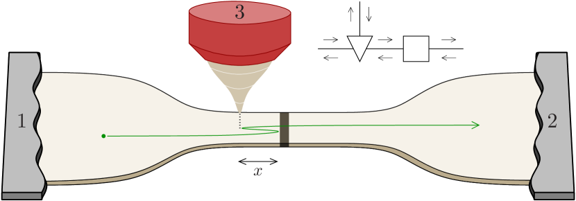
Figure 1: One-dimensional conductor with a scattering region (represented by a dark area) coupled to two terminals, 1 and 2, and to a third one via a scanning tip at $x$. Each terminal, $i$, is characterised by an electrochemical potential $\mu_{i}$ and a temperature $T_{i}$. Electron trajectories with multiple internal reflections (one of them is represented by the green arrow) interfere, breaking the conductor electron-hole symmetry. The inset represents the scattering problem schematically. The tip ($\triangledown$) and the scatterer ($\square$) are connected by a single channel.

Here we investigate how a thermoelectric response may be induced into a perfectly symmetric conductor (hereafter called simply conductor) by a mechanism based on quantum interference only. Transport in the conductor is defined by an energy-independent scattering region (hereafter called the scatterer) which does not yield any thermoelectric response on its own. In this sense we say the response is extrinsic to the conductor. As sketched in Fig. 1, we assume the third terminal to be a scanning tunneling probe Binnig and Rohrer (1987) that injects heat but on average no charge into the conductor. Such a heat source can furthermore be actively connected/disconnected. The overall response will hence depend on the tip position $x$ with respect to the scatterer. In particular, the tip presence induces interference patterns Hasegawa and Avouris (1993); Crommie et al. (1993a, b) which are measured by the probe electrochemical potential. They are understood in terms of multiple scattering trajectories between the tip and the scatterer Büttiker (1989). An example of such a trajectory with multiple internal reflections is shown as a green arrow in Fig. 1. The kinetic phase accumulated in these trajectories is sufficient to generate a thermoelectric current, an effect discussed in quantum Hall junctions Vannucci et al. (2015) and which-path interferometers Hofer and Sothmann (2015); Samuelsson et al. (2017); Haack and Giazotto (2019); Marchegiani et al. (2020a).

Currents in response to local heating have been recently measured in low dimensional systems via electronic injection Chen et al. (2012); Harzheim et al. (2018); Fast et al. (2020); Gächter et al. (2020), laser illumination Xu et al. (2010); Lemme et al. (2011); Zolotavin et al. (2017) or nanoheaters Mitra et al. (2021). Transport is there dominated by the diffusion of the electron-hole excitations across a potential barrier, what can be interpreted as a nanoscale version of current induced by Landauer blowtorches Landauer (1988); Büttiker (1987); van Kampen (1988). We assume a simple phenomenological description that intentionally neglects this effect (relying on the intrinsic response of the conductor) in order to isolate the contribution of quantum interference. We do this by considering a pointlike scatterer with no internal structure. More realistic descriptions of experimental situations would require the extension of our model to include configurations with more complex scattering properties Fleury et al. (2021). Different types of probes can also be considered Park et al. (2013); Menges et al. (2016); Steinacher et al. (2018); Marguerite et al. (2019).

Experimentally, signatures of oscillations appear overimposed to the intrinsic nonlocal Peltier coefficient of graphene constrictions in Ref. Harzheim et al. (2018). Scanning gate microscopes Sellier et al. (2011); Gorini et al. (2013); Steinacher et al. (2018) were also recently shown to induce interference fringes in the local thermopower of a quantum point contact Brun et al. (2019). Phase-dependent thermopower oscillations were as well reported in hybrid normal-superconducting interferometers Eom et al. (1998); Parsons et al. (2003), albeit of very different nature Jacquod and Whitney (2010); Kalenkov and Zaikin (2017).

In nonideal configurations, electrons may be affected by events where their phase coherence is lost. A description of the effect of incoherent processes in scattering theory is traditionally done by incorporating additional probe terminals. This approach dates back to the work of Engquist and Anderson Engquist and Anderson (1981) and was later refined by Büttiker for quantum coherent conductors Büttiker (1986, 1988). Such probes are standardly used to model voltage or temperature measurements, or the effect of inelastic scattering when electrons relax energy in the probe before being reinjected into the conductor. Analogously, quasi-elastic probes have been proposed to describe decoherence de Jong and Beenakker (1996) when particle currents are conserved at any energy in the probe. However, these probes are invasive in the sense that they introduce additional backscattering in the system: together with phase randomization, they involve momentum relaxation Büttiker (1991). This problem is irrelevant in disordered de Jong and Beenakker (1996) or chiral Pilgram et al. (2006); Förster et al. (2007) systems, but makes such backscattering-inducing probes unsuitable to describe pure dephasing in ballistic conductors. A few works address this issue Büttiker (1991); Datta (1995); Knittel et al. (1999); Li and Yan (2002); Golizadeh-Mojarad and Datta (2007). We consider the two types of probes (conserving and nonconserving momentum) separately. This way, we are first of all able to isolate the effect of pure dephasing on the interference fringes. The comparison of pure dephasing and quasi-elastic probe models gives useful insights into the relevant transport mechanisms. Furthermore, thermometer probes are used to describe (electron-electron) inelastic scattering processes and additionally to measure the effective temperature in the conductor, which is tip position-dependent.

The paper is organized as follows. In Sec. II we use scattering theory to describe the transport coefficients, which are analyzed in the linear response in Sec. III. Numerical results are shown in Sec. IV. Additional probes are included in Sec. V to describe (momentum conserving and nonconserving) dephasing and temperature probes. Conclusions are discussed in Sec. VI.

II Scattering theory

A simple and transparent description of the transport problem is given in terms of the scattering formalism for noninteracting electrons Sivan and Imry (1986); Streda (1989); Butcher (1990); van Houten et al. (1992). We adopt here a phenomenological approach where each component of the conductor is described by a minimal scattering matrix imposed by symmetry arguments. This allows us to identify the relevant interference processes involved in the three-terminal thermoelectric response.

II.1 Scattering matrices

We consider a single-channel one-dimensional conductor connected to two electronic leads, 1 and 2. Transport is assumed to be ballistic except for the presence of a scattering region (represented by a dark stripe in Fig. 1) at $x=0$ where electrons can be reflected. For concreteness, we will call this region the barrier in the following. We want a bare-bone conductor lacking any intrinsic thermoelectric response. This is the case if the barrier has no structure, with an energy-independent reflection probability $R$; see e.g., Ref. Benenti et al. (2017). Its scattering matrix can then simply be written as

$$\displaystyle{S^{\square}=\left(\begin{array}[]{cc}\sqrt{R}\text{e}^{i\phi}&\sqrt{1{-}R}\text{e}^{i(\pi+\phi)/2}\\ \sqrt{1{-}R}\text{e}^{i(\pi+\phi)/2}&\sqrt{R}\\ \end{array}\right),}$$ (3)

including the phase $\phi$.

Electrons are injected into the conductor by a scanning tunneling microscope, see Fig. 1, which we model as a pointlike beam splitter Büttiker (1989) at $x$ coupled to terminal 3. Assuming for simplicity that electrons from the tip are injected symmetrically into the other two branches of the beam splitter, we get a scattering matrix $S^{\triangledown}_{ij}=\sigma_{ij}^{\triangledown}e^{i(\delta_{i}+\delta_{j})}$, with the orthogonal matrix Büttiker et al. (1984):

$$\displaystyle{\sigma^{\triangledown}=\left(\begin{array}[]{ccc}-\eta_{-}/2&\eta_{+}/2&\sqrt{\varepsilon}\\ \eta_{+}/2&-\eta_{-}/2&\sqrt{\varepsilon}\\ \sqrt{\varepsilon}&\sqrt{\varepsilon}&\eta_{-}{-}1\\ \end{array}\right),}$$ (7)

where $\eta_{\pm}=1\pm\sqrt{1-2\varepsilon}$. The phases $\delta_{i}$ preserve the unitarity of $S^{\triangledown}$. The real parameter $\varepsilon\in[0,1/2]$ represents the tip-conductor coupling. In the limit $\varepsilon=0$, the tip and the conductor are separate systems. The opposite limit, $\varepsilon=1/2$, describes the case in which the tip has no internal reflection, such that all electrons from the tip terminal are (equally) transmitted into the conductor channels.

The scattering matrix of the whole system is obtained by composing the two matrices $S^{\triangledown}$ and $S^{\square}$ as explained in Appendix A. The local partial densities of states are different depending on whether the tip is on the left or on the right hand side of the barrier Gramespacher and Büttiker (1997, 1999), hence leading to different scattering matrices, $S^{-}$ and $S^{+}$, respectively.

Let us first consider the tip on the left side ($x<0$), as shown in Fig. 1. The second element of the outgoing waves of the tip is connected to the first element of the incoming waves of the conductor scattering region. Along the way between the tip and the scatter, they accumulate a phase $k|x|$ for wavenumber $k$. In this case, the transmission probabilities ${\cal T}_{ij}^{\pm}=|S_{ij}^{\pm}|^{2}$ read

$${\cal T}_{12}^{-}{=}\frac{(1{-}R)(\eta_{+}{-}\varepsilon)}{2{\cal A}},\quad{\cal T}_{13}^{-}{=}\frac{\varepsilon({\cal A}{+}\zeta)}{\cal A},\quad{\cal T}_{23}^{-}{=}\frac{(1{-}R)\varepsilon}{{\cal A}}.$$ (8)

They acquire an oscillatory behaviour due to the interference of trajectories with multiple internal reflections between the tip and the barrier, contained in

$${\cal A} =1+R(\eta_{-}{-}\varepsilon)/2\pm\sqrt{R}\eta_{-}\cos\chi$$ (9)

$$\zeta =R(\eta_{+}{+}\varepsilon)/2\pm\sqrt{R}\eta_{+}\cos\chi,$$ (10)

with $\chi=\chi_{0}^{-}+2k\left|x\right|$ and the phase $\chi_{0}^{-}=2\delta_{2}+\phi$ introduced by the two scatterers. Note that choosing the sign of the last term in the coefficients ${\cal A}$ and $\zeta$ simply adds a phase $\pi$ to $\chi$. In the following, we choose $+$. Such coefficients depend on energy via the momentum of the propagating electron, $k=\sqrt{2m(E-U_{0})}/\hbar$, where $U_{0}$ is the local potential energy, which we assume constant: $U_{0}=0$, for simplicity.

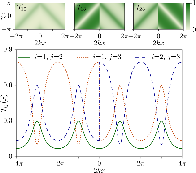
Figure 2: Transmission probabilities ${\cal T}_{ij}={\cal T}_{ji}$ between terminals $i$ and $j$ as functions of the tip position and the phase $\chi_{0}$, for $\varepsilon=R=1/2$. They are periodic in $2kx$ for $x$ not changing sign. When the tip crosses $x=0$, the roles of terminals 1 and 2 are exchanged. The lower panel shows cuts at $\chi_{0}=0$.

In the case that $x>0$ (when the tip is on the right side of the barrier), we obtain $S^{+}$ by exchanging 1$\leftrightarrow$2 in the indices of $S^{-}$, cf. Eq. (8), and replacing $\chi_{0}^{-}$ by $\chi_{0}^{+}=2\delta_{1}$. For convenience, we consider the symmetric case $\delta_{1}=\delta_{2}$ and $\phi=0$, where $\chi_{0}\equiv\chi_{0}^{+}=\chi_{0}^{-}$ (except when explicitly stated). The general expression of the transmission probabilities ${\cal T}_{ij}$ for electrons injected from terminal $j$ to reach terminal $i$ is then obtained by combining

$${\cal T}_{ij}={\cal T}_{ij}^{-}\Theta(-x)+{\cal T}_{ij}^{+}\Theta(x)$$ (11)

with the Heaviside function $\Theta(x)$. They are plotted in Fig. 2 as functions of the tip position (determining the accumulated phase) and $\chi_{0}$. Note that the discontinuity of the probabilities ${\cal T}_{13}$ and ${\cal T}_{23}$ at $x=0$ is due to having a point-like scattering region.

II.2 Currents

With all these, we write the particle and heat currents injected from the different terminals:

$$I_{i} =\int dE\leavevmode\nobreak\ {\cal I}_{i}(E)$$ (12)

$$J_{i} =\int dE\leavevmode\nobreak\ (E-\mu_{i}){\cal I}_{i}(E),$$ (13)

with the current densities given by

$${\cal I}_{i}(E)=\frac{2}{h}\sum_{j}{\cal T}_{ji}[f_{i}(E){-}f_{j}(E)],$$ (14)

where $f_{i}=1/\{1+\exp{[(E-\mu_{i})/k_{\text{B}}T_{i}}]\}$ is the Fermi function of terminal $i$, $h$ and $k_{B}$ are the Planck and Boltzmann constants, and the factor $2$ takes into account spin degeneracy. The sum is over every terminal in the system. For our particular case they read, for $x<0$:

$${\cal I}_{2} =\frac{2(1{-}R)}{h}\frac{1}{\cal A}\left[\varepsilon(f_{2}{-}f_{3})+\frac{\eta_{+}{-}\varepsilon}{2}(f_{2}{-}f_{1})\right]$$ (15)

$${\cal I}_{3} =\frac{2\varepsilon}{h}\frac{1}{\cal A}\left[({\cal A}{+}\zeta)(f_{3}{-}f_{1}){+}(1{-}R)(f_{3}{-}f_{2})\right].$$ (16)

The expression for terminal 1 is obtained by particle conservation, ${\cal I}_{1}=-{\cal I}_{2}-{\cal I}_{3}$. The currents hence adopt the oscillatory behaviour of the coefficients ${\cal A}$ and $\zeta$ Hasegawa and Avouris (1993); Crommie et al. (1993a, b).

The transport problem is solved by assuming probe boundary conditions for the tip. Throughout this work, we will assume that the tip is a voltage probe, i.e., its electrochemical potential $\mu_{3}$ adapts to the condition $I_{3}=0$, so it does not inject charge in the system on average. The probe is sensitive to the phase accumulated in the conductor and the measured electrochemical potential oscillates with the distance to the barrier Büttiker (1989).

II.3 Conservation laws and thermodynamics

Under these conditions, charge conservation is expressed only by the conductor terminals

$$I_{1}+I_{2}=0,$$ (17)

so the generated particle current is unambiguously defined by one of them. Differently, energy conservation involves all three terminals. In terms of the heat currents, it is written as

$$J_{1}+J_{2}+J_{3}=P$$ (18)

and involves the electric power:

$$P=-(\mu_{2}-\mu_{1})I_{2}.$$ (19)

We use the convention that $P$ is positive when electrons flow against the chemical potential difference. When this occurs due to heating of terminal $i$, $T_{i}=T+\delta T_{i}$, the system works as a converter of heat into useful power, with an efficiency $\eta_{i}=P/J_{i}$. Scattering theory respects the second law Benenti et al. (2017), so it can be shown that $\eta_{i}\leq\eta_{C}$, with the Carnot efficiency $\eta_{C}=1-T/T_{i}$.

We anticipate that, when coupling the system to fictitious probes in Sec. V, the imposed boundary conditions will involve that neither particle nor heat currents are injected. Therefore the above conservation laws for average currents, Eqs. (17) and (18), will not be affected.

III Three-terminal thermoelectric response

An important observation from Eq. (15) is that the thermoelectric response of the conductor vanishes when the tip is not coupled to it. We can easily verify that for $\varepsilon=0$, we have ${\cal A}=1$, and the current reduces to that of an energy-independent two-terminal resistor: $I_{2}=2(1{-}R)(\mu_{2}-\mu_{1})/h$. Namely, it is independent of the temperatures $T_{1}$ and $T_{2}$ of terminals 1 and 2, up to charge accumulation effects in the nonlinear regime Whitney (2013); Sánchez and López (2013); Meair and Jacquod (2013) that we neglect here. This ensures that the thermoelectric response discussed below is induced by the presence of the tip only.

To have a finite thermoelectric response, the transmission probabilities ${\cal T}_{ji}$ need to depend on energy. This dependence is introduced by the oscillatory term in ${\cal A}$ and $\zeta$ as soon as $R\neq 0$: if $R=0$ (a perfect conductor), we have ${\cal A}=1$ and $\zeta=0$, and hence $I_{2}$ and $I_{3}$ are insensitive to the temperatures $T_{1}$, $T_{2}$, and $T_{3}$. The general problem of solving the integrals in Eqs. (12) and (13) with the corresponding boundary conditions is complex and will be solved numerically in Sec. IV. However, we gain some useful insight by performing a linear response analysis, together with a Sommerfeld expansion at low temperature.

III.1 Linear response analysis

Let us assume small electrochemical potential and temperature differences between the different terminals, $\delta\mu_{i}=\mu_{i}-\mu\ll k_{\text{B}}T$ and $\delta T_{i}=T_{i}-T\ll T$ with respect to the reference electrochemical potential $\mu$ and temperature $T$. The currents are then expanded as

$$I_{i} =\sum_{j}\left[G_{ij}(\mu_{i}-\mu_{j})+L_{ij}(T_{i}-T_{j})\right]$$ (20)

$$J_{i} =\sum_{j}\left[M_{ij}(\mu_{i}-\mu_{j})+K_{ij}(T_{i}-T_{j})\right],$$ (21)

where $G_{ij}=2g_{ij}^{(0)}$ and $K_{ij}=2g_{ij}^{(2)}/T$ are the multiterminal particle and heat conductances, while $L_{ij}=2g_{ij}^{(1)}/T$ and $M_{ij}=2g_{ij}^{(1)}$ are the multiterminal thermoelectric coefficients related to the Seebeck and Peltier effects Butcher (1990), respectively. We write them in terms of the integrals

$$g_{ij}^{(n)}=\frac{1}{h}\int{dE}\frac{(E-\mu)^{n}}{4k_{\text{B}}T}{\cal T}_{ji}(E)\cosh^{-2}\left(\frac{E-\mu}{2k_{\text{B}}T}\right)$$ (22)

which make the Onsager reciprocity relations Casimir (1945) explicit via ${\cal T}_{ji}={\cal T}_{ij}$.

With these response coefficients, we first obtain the probe electrochemical potential by imposing $I_{3}=0$:

$$\mu_{3}=\frac{1}{G_{13}+G_{32}}\sum_{l}[G_{3l}\mu_{l}+L_{3l}(\delta T_{l}-\delta T_{3})],$$ (23)

with the sum limited to the conductor terminals $l=1,2$. Replacing it in the expression for the current in the conductor and using $\sum_{j}L_{ij}=0$ (a consequence of charge conservation), we get

$$I_{2}=\left(G_{21}+\frac{G_{13}G_{23}}{G_{13}+G_{23}}\right)(\mu_{2}-\mu_{1})-\sum_{j}{\cal L}_{2j}\delta T_{j},$$ (24)

with the thermoelectric responses

$${\cal L}_{2j}=L_{2j}+\frac{G_{23}L_{3j}}{G_{13}+G_{23}}.$$ (25)

The current $I_{1}$ is obtained by replacing 1$\leftrightarrow$2 and one checks that $I_{1}=-I_{2}$. One can readily see that while the response matrices $G$, $L$, $M$ and $K$ are symmetric, this is not the case, in general, for the thermoelectric responses when not all terminals are equivalent (e.g., one of them is a probe) Sánchez and Serra (2011): then ${\cal L}_{ij}\neq{\cal L}_{ji}$. Note that this implies the possibility of thermoelectric current rectification in the linear regime, in the presence of heat leakage induced by inelastic scattering at the tip terminal Sánchez and Serra (2011). In our case, $L_{31}$ and $L_{32}$ will be finite due to interference, as discussed above. The coefficients for heat currents are given in Appendix B.

We can also verify that ${\cal L}_{2j}=0$ if $\varepsilon=0$ or $R=0,1$, because $g_{ij}^{(1)}=0$ if ${\cal T}_{ji}$ does not depend on energy.

III.2 Sommerfeld expansion

A convenient way to picture the relevant processes is to perform a Sommerfeld expansion (see e.g., Ref. Benenti et al. (2017)) on the linear regime coefficients. For small $k_{\text{B}}T/\mu$, the integrals are evaluated as $g_{ij}^{(0)}={\cal T}_{ji}(\mu)/h$, $g_{ij}^{(1)}=q_{\rm H}{\cal T}_{ji}^{\prime}(\mu)$ and $g_{ij}^{(2)}=q_{\rm H}{\cal T}_{ji}(\mu)$, where $q_{\rm H}=\pi^{2}k_{\text{B}}^{2}T/3h$ is the quantum of thermal conductance Pendry (1983). This is a good approximation when the energy dependence of the transmission coefficient is smooth around $\mu$. In our system, the oscillatory behaviour of ${\cal T}_{ji}$ introduces additional limitations to the applicability of the approximation. For a fixed tip position, they oscillate with a period that depends on $\mu$. Hence, the Sommerfeld expansion stays valid when $\nu_{\text{F}}|x|\ll 1/k_{\text{B}}T$ and thermal fluctuations remain negligible (see Appendix C). Here, $\nu_{\text{F}}=\sqrt{2m/\mu}/h$ is the 1D density of states at the Fermi energy. For this reason, we will restrict our analysis in this section to tip distances close to $x=0$.

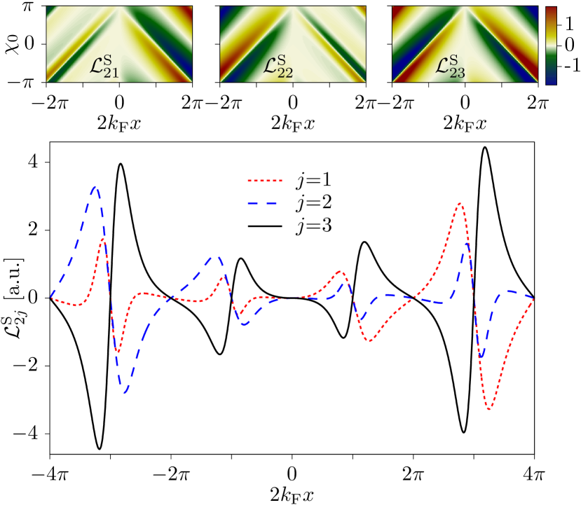
Figure 3: Linear response coefficients ${\cal L}_{2j}$ of the current at terminal 2 when increasing the temperature of terminal $j$ by $\delta T_{j}=\delta T$ as described by a Sommerfeld expansion, for the same parameters as in Fig. 2, with the Fermi wavenumber $k_{\rm F}$. The lower panel shows cuts at $\chi_{0}=0$ for a doubled range of tip positions.

The resulting thermoelectric coefficients, ${\cal L}_{2j}^{\rm S}$, are plotted in Fig. 3, showing their dependence on the tip position and on the scattering phase $\chi_{0}$. Clearly, the discontinuity of the transmission probabilities at $x=0$ (see Fig. 2) has an effect in the transport coefficients, which depend on the sign of $x$. However, we note that transport coefficients are reciprocal: ${\cal L}_{ll^{\prime}}^{\rm S}(x,\chi_{0}^{\pm})={\cal L}_{l^{\prime}l}^{\rm S}(-x,\chi_{0}^{\mp})$ in the longitudinal terms, and ${\cal L}_{l3}^{\rm S}(x,\chi_{0}^{\pm})={\cal L}_{l^{\prime}3}^{\rm S}(-x,\chi_{0}^{\mp})$ in the crossed ones, for $l,l^{\prime}=1,2$ and $l\neq l^{\prime}$ (remember that ${\cal L}_{1i}^{\rm S}=-{\cal L}_{2i}^{\rm S}$).

We observe a series of irregular sawtooth-like oscillations as the tip scans the conductor. These are a hallmark of resonances arising from interference. The oscillations shape and sign change depending on which terminal is heated, but they always vanish at $\chi_{\rm F}\equiv 2k_{\rm F}x+\chi_{0}=n\pi$. Remarkably, the longitudinal responses have an additional series of nodes when the tip is in between the barrier and the hot terminal (see ${\cal L}_{21}$, for $x<0$, and ${\cal L}_{22}$, for $x>0$). This is possible because the thermoelectric response of the probe (given by its electrochemical potential) has an opposite (and larger) contribution when it is close to the hot terminal, and adds up when it is separated from it by the barrier. We can check this by noticing that $\mu_{3}\propto L_{3l}\delta T_{l}\propto{\cal T}_{3l}^{\prime}(\mu)\delta T_{l}$ and that ${\cal T}_{13}^{\prime}$ and ${\cal T}_{23}^{\prime}$ have opposite signs, cf. Fig. 2. Then, at a fixed tip position the two terms in Eq. (25) have the same or opposite contributions for $j=1$ and $j=2$, in which case they eventually cancel out. Note also that the highest oscillations (in absolute value) correspond to the nonlocal case with a hot tip, while the lowest are those where the hot terminal is on the same side as the tip.

The Sommerfeld expansion also predicts that the generated current increases with the tip-barrier distance, as can be appreciated in Fig. 3. This is understood by noticing that all thermoelectric coefficients scale as $L_{ij}^{\rm S}\propto{\cal T}^{\prime}_{ji}(\mu)\propto\partial_{E}(k|x|)|_{\mu}\propto|x|$. In particular, for $x<0$,

$${\cal L}_{2j}^{\rm S} =q_{\mathop{\mathrm{H}}}\frac{4\pi(1-R)\sqrt{R}}{{{\cal A}}_{\text{F}}({{\cal A}}_{\text{F}}+\zeta_{\text{F}}+1-R)}C_{j}x\nu_{\text{F}}\sin\chi_{\text{F}},$$ (26)

where all quantities with a sub-index F are evaluated at the Fermi energy, and

$$C_{1} =2\varepsilon(\eta_{+}-\varepsilon R)+(\varepsilon-\eta_{+})\eta_{-}({{\cal A}}_{\text{F}}+\zeta_{\text{F}}+1-R)$$

$$C_{2} =(\eta_{+}+\varepsilon)({{\cal A}}_{\text{F}}+\zeta_{\text{F}}+1-R)-2\varepsilon$$ (27)

$$C_{3} =2\varepsilon{{\cal A}}_{\text{F}}.$$

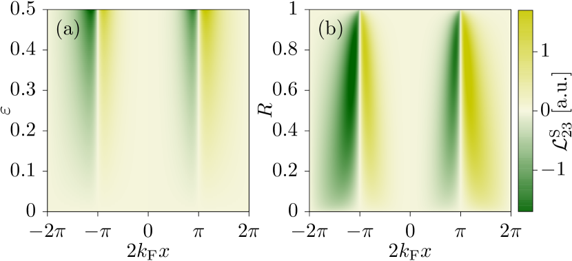
Figure 4: Dependence of the nonlocal linear response coefficient ${\cal L}_{23}^{\rm S}$ on (a) the tip coupling $\varepsilon$ (for $R=0.75$) and on (b) the conductor reflection coefficient $R$ (for $\varepsilon=0.5$). In both cases, $\chi_{0}=0$.

Figure 4 shows the dependence of the nonlocal term, ${\cal L}_{23}^{\rm S}$, on the coupling parameters $\varepsilon$ and $R$. It increases with the coupling to the tip, $\varepsilon$, and is maximal for $\varepsilon=1/2$, see Fig. 4(a). As expected, the response vanishes both for $R=0$ and $R=1$, when there is no interference, and is maximal around $R\approx 3/4$, see Fig. 4(b).

IV Numerics

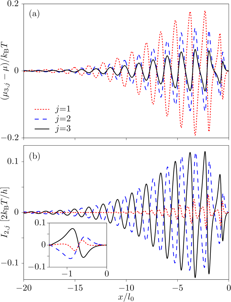
Figure 5: (a) Electrochemical potential measured by the tip, $\mu_{3,j}$, and (b) thermoelectric current, $I_{2,j}$, when the temperature of terminal $j$ is increased by $\delta T=T/2$. The inset in panel (b) shows a zoom on the currents at short distances. Parameters: $\varepsilon=R=0.5$, $\chi_{0}=0$, $U_{0}=0$, and $\mu=20k_{\text{B}}T$.

Numerically evaluating the integrals in Eqs. (12) and (13), under the condition that $\mu_{3}$ is such that $I_{3}=0$, affords a more complete understanding. We restrict in the following to $x<0$, so charge currents are given by Eqs. (15) and (16). We do this for different configurations, depending on which terminal $j$ holds a temperature increase ${\mathop{\delta{T}}}$ (and assuming $\mu_{1}=\mu_{2}=\mu)$. This results in different probe electrochemical potentials, $\mu_{3,j}$ and currents $I_{2,j}$. The result is plotted in Fig. 5 as a function of the tip position, with $l_{0}=\hbar/\sqrt{8mk_{\rm B}T}$. The electrochemical potential of the probe oscillates around $\mu$, cf. Fig. 5(a). Note that when terminal 1 is hot, the electrochemical potential has the opposite sign with respect to the other cases. It also gives the oscillations with the largest amplitude. This is in contrast with the generated current in Fig. 5(b): the smaller the probe response, the largest the current is.

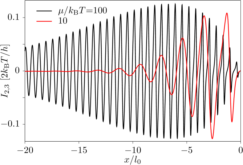
Figure 6: Dependence of the nonlocal thermoelectric current ($T_{3}=T+{\mathop{\delta{T}}}$) on the electrochemical potential $\mu$, for otherwise the same parameters of Fig. 5.

The currents in Fig. 5(b) reproduce the behaviour expected from the Sommerfeld expansion ($I_{2,j}\approx-{\cal L}_{2,j}^{\rm S}{\mathop{\delta{T}}}$) at short distances, compare Fig. 3 with the zoom in the inset of Fig. 5(b). The same pattern repeats over $x$, with the oscillation amplitudes modulated by the distance. For short distances, the amplitude increases linearly, in agreement with the Sommerfeld expansion. However, there is a crossover to longer distances where the currents decrease. In this regime, the energy dependence of the transmission probabilities around the Fermi energy becomes sensitive to the electrochemical potential $\mu$ through the argument $2k|x|$ of the oscillating term, see Eqs. (8) to (10). The energy separation of the oscillations decreases with increasing $|x|$ to a point where they are averaged out in the integration. See Appendix C for a more detailed discussion of this point. This is confirmed by the results shown in Fig. 6: For larger ratios $\mu/k_{\text{B}}T$, the interference pattern survives at longer distances, and the linear increase for low $x$ can also be more clearly appreciated. For lower $\mu/k_{\text{B}}T$, thermal fluctuations dominate at shorter distances. However, the maximal generated currents are of the same order in both cases.

IV.1 Active tip: Nonlocal thermoelectric current

Let us focus on the case where the tip is hotter, $T_{3}=T+{\mathop{\delta{T}}}$, while $T_{1}=T_{2}=T$ and $\mu_{1}=\mu_{2}=\mu$. It is interesting to compare this configuration with typical thermocouples where two junctions separate a central hot region (in contact with the heat source) from the rest of the conductor. Those two junctions are furthermore responsible for the separation of electron-hole excitations. Mesoscopic analogs maintain this structure Jaliel et al. (2019). Our case is different, since the conductor has a single barrier. The conductor-tip coupling provides the mechanism of heat injection from the source (terminal 3), as well as that for thermoelectric current generation. Local thermalization of electrons is not required, i.e., there is no need to define an internal temperature distribution in the conductor (we will however come back to this point in Sec. V). Transport is hence affected by the nonequilibrium properties of the injected electrons.

In this sense, the thermoelectric properties and the heat source are external to the circuit where current is generated. The tip in a voltage probe configuration injects electron-hole excitations into the system, hence no charge (on average) but heat. In their propagation between the tip and the barrier, electron and hole quasiparticles acquire different phases, which gives an effect due to the interference of the possible internal reflections. The tip position $x$ hence marks the point where both nonequilibrium excitations and electron-hole asymmetry are induced. The relevance of the phase coherence will be further explored in Sec. V by introducing dephasing probes phenomenologically.

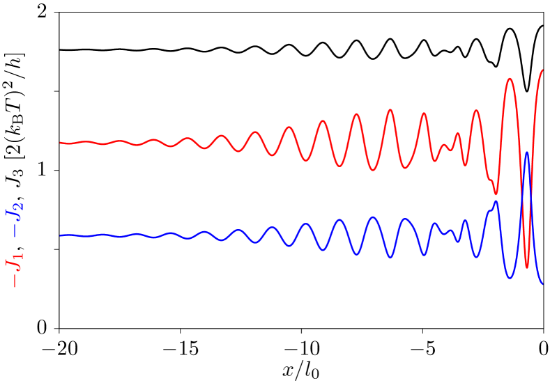
Figure 7: Heat currents into the different terminals, $J_{i}$, when the tip temperature is hot, $T_{3}=T+{\mathop{\delta{T}}}$, for the same parameters as in Fig. 5.

The heat currents due to the coupling to the hot tip are also affected by the interference pattern, as shown in Fig. 7. Note that, as for $I_{2,1}$, a double oscillation is apparent for low $x$ that we similarly attribute to the tip probe conditions, see the competition of terms in the linear coefficients in Appendix B. However, they are always finite. As expected, for the tip being far from the barrier, the heat current is larger in the terminal that is the closest to the tip i.e., $J_{1}>J_{2}$ for $x<0$. As the tip approaches the barrier, oscillations appear with opposite phase in terminals 1 and 2 and increase their amplitude to a point that eventually makes the heat current through the barrier larger than that flowing directly to the nearest terminal ($J_{2}>J_{1}$, in this case).

As there is always one terminal into which electrons flow without being scattered, a large amount of heat will be absorbed by the conductor without contributing to generating a charge current. For this reason, the injected heat current, $J_{3}$, is expected to be much larger than the power generated in the nonlocal thermoelectric conversion, $P=-(\mu_{2}-\mu_{1})I_{2}$. We show this in Figs. 8(a) and 8(b) for the parameters where the linear response coefficient ${\cal L}^{S}_{23}$ is maximal within Sommerfeld, i.e., with $\varepsilon=0.5$ and $R=0.75$, see Fig. 4(b). Indeed, we find that the efficiency $\eta_{3}=P/J_{3}$ is smaller than 2.6% of the Carnot efficiency, $\eta_{C}=1-T/T_{3}$, for the chosen parameters, see Fig. 8(c). Interestingly, due to the coherent oscillations, the system behaves as a bipolar converter able to produce power for opposite bias voltages but the same temperature configuration, only by shifting the position of the tip.

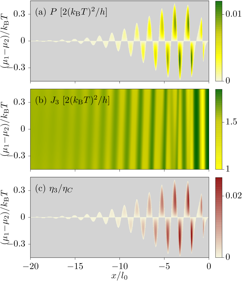
Figure 8: Performance of the nonlocal thermoelectric effect. (a) Generated power, (b) injected heat current from the hot tip (with $T_{3}=T+\delta T$), and (c) efficiency of the heat to power conversion, for $\varepsilon=0.5$ and $R=0.75$. Other parameters are as in Fig. 5. The light-grey background in (a) and (c) marks regions where power is dissipated, $P<0$.

We speculate that the performance will be improved if the tip is placed between two barriers. Such configuration furthermore introduces an additional interference mode. However, a detailed investigation of this particular issue is out of the scope of this paper.

IV.2 Passive tip: Thermoelectric diode

A longitudinal thermoelectric effect appears in the case that the hot terminal is in the conductor (either terminal 1 or 2) provided the coupling to the tip is finite. It was discussed above that the response is asymmetric and depends on the position of the tip with respect to the barrier and the heat source [$I_{1,2}(x)=I_{2,1}(-x)\neq I_{2,1}(x)$], cf. Figs. 3 and 5. This is possible because energy is relaxed in the voltage probe by means of inelastic scattering Büttiker (1986). The probe then induces a thermoelectric rectification effect even in the linear regime Rosselló et al. (2017).

The asymmetry does not only affect the magnitude of the currents: To be more precise, we recall that the number of current sign changes with the tip position is doubled when the hot terminal and the tip are on the same side of the barrier; see, e.g., Fig. 5(b). Let us restrict for clarity to the case $x<0$ (the case of positive tip positions is obtained by changing terminals 1 and 2 everywhere in the discussion). In that case, there exist some positions $x$ of the tip where $I_{2,1}(x)=0$ while $I_{2,2}(x)\neq 0$, i.e., charge flows or not through the conductor, depending on which of its terminals is coupled to the heat source, which is very much what one expects of an ideal diode when reversing the sign of the applied voltage. The system then works as an ideal thermoelectric diode.

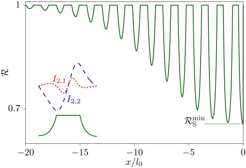
Figure 9: Thermoelectric rectification coefficient ${\cal R}$ for the currents plotted in Fig. 5(b). A zoom at small $x$ (coinciding with the inset of Fig. 5) is shown in the inset for clarity. For short distances, ${\cal R}$ oscillates between 1 and ${\cal R}_{\text{S}}^{\rm min}$, as described by the Sommerfeld expansion in Eq. (29).

To quantify the behaviour of a diode, one compares the forward current $I_{\rightarrow}=I_{2,1}$ measured in terminal 2 when 1 is hot, and the backward one $I_{\leftarrow}=I_{1,2}$ in the opposite case. Remember we have $I_{1,l}=-I_{2,l}$. We parametrize its performance by means of the rectification coefficient:

$${\cal R}=\frac{|I_{\rightarrow}-I_{\leftarrow}|}{|I_{\rightarrow}|+|I_{\leftarrow}|},$$ (28)

which gives ${\cal R}=1$ in the mentioned ideal case and ${\cal R}=0$ if there is no rectification. As shown in Fig. 9 and its inset, the zeros of $I_{2,1}$ define regions where the thermoelectric current flows in the same direction irrespective of the sign of the temperature gradient along the conductor, resulting in the plateaus with ${\cal R}=1$. Similar features may appear for the heat currents in interacting quantum dot systems because the third terminal acts as a heat sink Sánchez et al. (2017). However, we emphasize that in our case, the rectified (particle) current is conserved in the conductor.

We note that for tip positions close to the barrier, the rectification coefficient is well described by the results of the Sommerfeld expansion

$${\cal R}_{\text{S}}=\frac{|C_{1}+C_{2}|}{|C_{1}|+|C_{2}|},$$ (29)

with the coefficients $C_{i}$ given in Eqs. (III.2). In this regime, the linear dependence of the currents with $x$ shown in Eq. (26) makes ${\cal R}_{\text{S}}$ vary between 1 and a constant value (i.e., independent of $x$), marked by ${\cal R}_{\text{S}}^{\rm min}$ in Fig. 9. As the current oscillations decrease with the distance (in a regime where the Sommerfeld expansion breaks down), the minima of ${\cal R}$ increase toward 1. In this regime there is a useless strong rectification of tiny currents.

V Additional probes

The phenomena discussed above arise from quantum interference. In real systems, electrons might however lose phase coherence while propagating along the conductor. It is hence important to explore the robustness of the phenomena to the presence of decoherence.

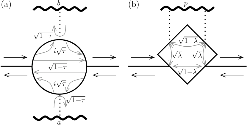
Figure 10: Representation of the scattering matrices for decoherence processes. (a) $S^{\ocircle}$ describes pure dephasing. Two fictitious probes, $a$ and $b$, are coupled via the dotted channels to the conductor in a chiral way: each of them absorbs and reinjects only left- or right-moving electrons with amplitude $i\sqrt{\tau}$. They have an internal reflection amplitude $\sqrt{1{-}\tau}$. (b) $S^{\Diamond}$ describes the coupling, with amplitude $\sqrt{\lambda}$, of an invasive probe terminal $p$ inducing backscattering. Depending on the boundary conditions, it is used to model quasielastic or inelastic scattering processes.

This is typically done by adding probe terminals to the region between the tip and the barrier. Electrons propagating along the conductor can be absorbed and reinjected by these probes, resulting in phase randomization. The desired properties are phenomenologically described depending on the characteristics of the coupling (given by a scattering matrix) and the boundary conditions imposed to the probe(s). We will consider two kinds of couplings, represented in Fig. 10. They differ in whether they introduce phase randomization without backscattering [$S^{\ocircle}$, cf. Fig. 10(a)], and are hence appropriate for describing pure dephasing, or whether they randomize momentum as well [$S^{\Diamond}$, cf. Fig. 10(b)]. The latter (which we refer to as invasive in the following) are good for describing decoherence induced by inelastic Büttiker (1986, 1988) and quasielastic scattering de Jong and Beenakker (1996). Furthermore, they serve as models of thermometers Engquist and Anderson (1981); Jacquet and Pillet (2012); Meair et al. (2014); Argüello-Luengo et al. (2015); Stafford (2016). Experimentally, spatially resolved nonequilibrium distribution Tikhonov et al. (2020) and temperature Halbertal et al. (2016, 2017); Marguerite et al. (2019) measurements have been achieved with more involved probes. A simple analytical treatment is however sufficient for our purposes here.

Hereafter, we use the two kinds of probes with different boundary conditions to model separately the effect of pure dephasing, of quasielastic scattering, and of a temperature probe inducing (electron-electron) inelastic scattering.

V.1 Pure dephasing

In order to take processes that only affect the phase into account (avoiding additional backscattering), we need a four-channel scattering matrix: two channels [represented by full lines in Fig. 10(a)] correspond to the partitioned channel of the conductor. The other two [dotted lines in Fig. 10(a)] are connected to two fictitious probes, $a$ and $b$, with probability $\tau$. The coupling of the probes to the conductor is chiral Büttiker (1991): each of them absorbs electrons from a different ingoing conductor mode and reinjects them in the opposite outgoing mode with the same energy. To mimic pure dephasing, we impose the boundary conditions ${\cal I}_{a}(E)={\cal I}_{b}(E)=0$, i.e. charge is conserved at every energy in each probe terminal. This way, after visiting the corresponding probe, where they lose their phase information, electrons continue propagating in the same direction with no energy being exchanged between system and probe.

We will only consider cases where the dephasing probes are placed between the tip and the barrier. Details on the scattering matrix $S^{\ocircle}$, as well as how the transmission probabilities are modified and the expressions for the resulting currents are given in Appendix D.

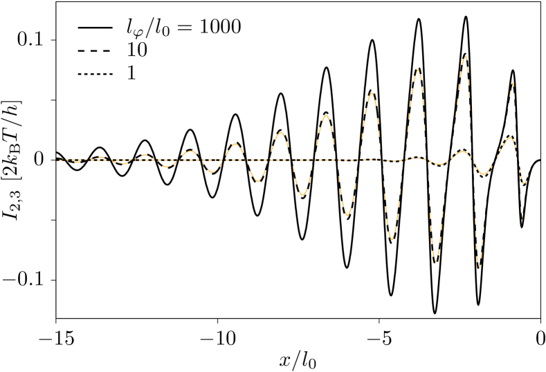
Figure 11: Effect of pure dephasing on the nonlocal thermoelectric current ($T_{3}=T+\delta T$), parametrized by the phase coherence length, $l_{\varphi}$, defined in Eq. (30). Parameters are as in Fig. 5, whose curve $I_{2,3}$ is the limit $l_{\varphi}\rightarrow\infty$ of this case. As there, $\delta T=T/2$. The cases with decoherence due to a (non momentum conserving) quasielastic scattering for the same values of the length defined in Eq. (31) are shown in orange, for comparison.

The probe conditions ${\cal I}_{a}(E)={\cal I}_{b}(E)=0$ are satisfied only if the probes acquire a nonequilibrium distribution, as discussed in Appendix D, see Eq. (72). The resulting nonlocal current is plotted in Fig. 11. We get a more physical insight of the effect of dephasing by introducing a phenomenological dephasing length defined as

$$\tau(x)=1-e^{-|x|/l_{\varphi}}.$$ (30)

That is, the phase coherence of the injected electrons is fully lost before any internal reflection occurs if the tip and the barrier are far enough ($|x|\gg l_{\varphi}$), as they will likely be absorbed by terminals $a$ or $b$. When the tip distance is of the order of the dephasing length, the loss of phase coherence between tip and barrier will only be partial. This is shown for various $l_{\varphi}$ in Fig. 11. The current vanishes for tip positions larger than $l_{\varphi}$, confirming the importance of the interference effect for having a nonlocal thermoelectric response. Conductors with a short coherence length will generate current only for tips in the close vicinity of the barrier.

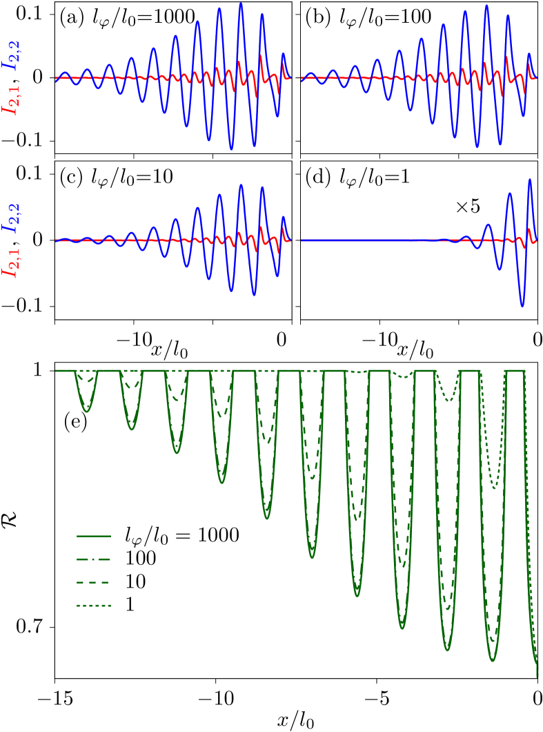
Figure 12: Dependence of (a)-(d) the longitudinal currents $I_{2,1}$ and $I_{2,2}$ and (e) the thermoelectric rectification coefficient ${\cal R}(x)$ on the phase coherence length due to pure dephasing, $l_{\varphi}$. All other parameters are as in Figs. 5 and 9, which correspond to taking $l_{\varphi}\rightarrow\infty$.

The longitudinal currents are affected by dephasing in a similar way, as shown in Fig. 12. As the coupling to the probes increases, the amplitude of the oscillations decreases. As the probes respect the electronic propagation, the different features of the currents $I_{\rightarrow}$ and $I_{\leftarrow}$ that resulted in the rectification properties discussed in Sec. IV.2 are maintained, see Fig. 12(a)-(d). As a consequence, we still find regions where the two currents have the same sign (and give ${\cal R}=1$). Furthermore, the rectification coefficient increases when the dephasing length decreases, see Fig. 12(e), with the drawback that the rectified currents become small.

V.2 Quasielastic scattering

Dephasing and/or decoherence can also be caused by processes that randomize both phase and momentum of the carriers. A minimal description of these processes is given by connecting the conductor to a single probe terminal, which we will label $p$, where electrons relax before being reinjected into the conductor Büttiker (1986), see Fig. 10(b). The coupling probability is in this case $\lambda$. Processes of different microscopic origins can be mimicked by imposing appropriate boundary conditions at the probe. We now consider elastic scattering, and discuss inelastic processes in Sec. V.3. We give details of the probe scattering matrix $S^{\Diamond}$ and the corresponding transmission probabilities ${\cal T}_{\alpha\beta}^{\lambda}$, as well as the expression for the resulting currents in Appendix E.

The fictitious probe terminal $p$ describes quasielastic dephasing by again imposing energy-resolved boundary conditions, ${\cal I}_{p}(E)=0$: the probe absorbs and reinjects electrons without changing their energy, but randomizing their phase and momentum de Jong and Beenakker (1996). As a result the probe acquires a nonequilibrium distribution, cf. Eq. (82).

A phenomenological phase coherence length $l_{\varphi}$ can also be defined in this case as

$$\lambda(x)=1-e^{-|x|/l_{\varphi}}.$$ (31)

Its effect on the nonlocal response is shown in Fig. 11, being almost indistinguishable from the case of pure dephasing, especially for short coherence lengths. However, we observe that the amplitude of the oscillations is most effectively reduced by the quasielastic scattering processes, due to the additional relaxation of momentum.

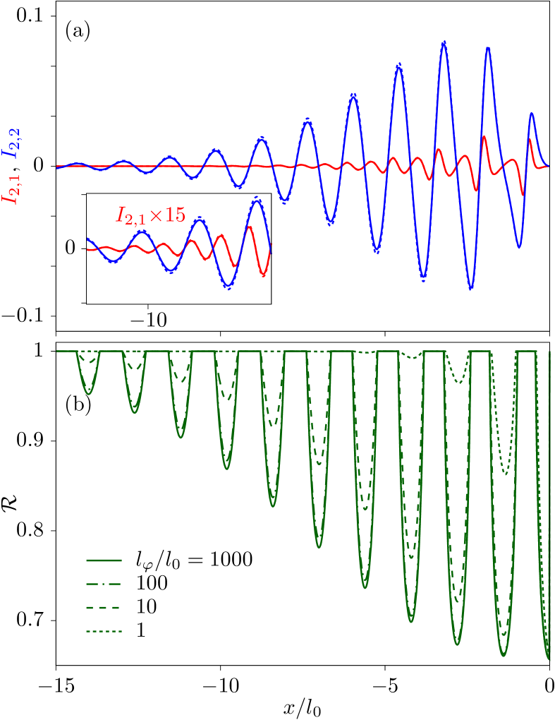
Figure 13: Effect of quasielastic scattering on the longitudinal response. (a) Longitudinal currents $I_{2,1}$ (full red line) and $I_{2,2}$ (full blue line), for $l_{\varphi}=10/l_{0}$. The case where the same $l_{\varphi}$ corresponds to pure dephasing is shown in dotted lines, see Fig. 12(c) for comparison. The inset shows a zoom of some oscillations. (b) Thermoelectric rectification coefficient ${\cal R}(x)$ for different coherence lengths. All other parameters are as in Figs. 5 and 9, which correspond to the case $l_{\varphi}\rightarrow\infty$.

Differently from the pure dephasing case of Sec. V.1, the probe introduces backscattering, which erases the information related to the terminal where electrons are injected. This however does not affect the diode effect appreciably. The asymmetry between $I_{\rightarrow}$ and $I_{\leftarrow}$ is also reduced but robust so as to still give a high rectification coefficient for strongly decoherent conductors, see Fig. 13(b). However this again occurs for vanishingly small currents.

V.3 Thermometer

Alternatively we can use the invasive probe described by the scattering matrix $S^{\Diamond}$ as a thermometer Engquist and Anderson (1981). For this, we assume that electrons entering the probe relax energy and thermalize due to inelastic scattering. The probe compensates this by increasing its temperature, so it does not inject any heat in the conductor. Mathematically, the electrochemical potential and temperature of the probe are adapted to the boundary conditions $I_{p}=J_{p}=0$, this time imposed to the average currents. Note the difference with the dephasing probe in Sec. V.2, which imposes ${\cal I}_{p}(E)=0$ to the energy-resolved particle current. The distribution of the probe, rather than being out of equilibrium locally as in Eq. (82) will be given by a Fermi distribution defined by the resulting $\mu_{p}$ and $T_{p}$. Other definitions of a local thermal probe can however be used Zhang et al. (2019).

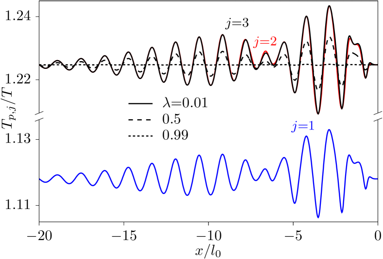
Figure 14: Temperature of the probe terminal when the temperature of terminal $j=1$ (blue), $j=2$ (red), and $j=3$ (black), is $T_{j}=1.5T$, with $\lambda=0.01$. Dashed and dotted lines show the case of a hot tip for increasing values of the coupling $\lambda$, as labeled. Same parameters as in Fig. 5.

As a thermometer, it is important that the probe does not have its own thermoelectric response, which is achieved by considering that the coupling $\lambda$ is an energy independent constant. Unlike the tip, this probe does not have spacial resolution, so it measures the effective temperature of the region between the tip and the scattering region not . Note that the electrochemical potential at the probe, $\mu_{p}$, is in general different from the one simultaneously measured by the tip, $\mu_{3}$. The measured temperature is shown in Fig. 14. The spacial modulation of the probe outcomes with the position of the tip shows a beating behaviour which reflects that of the heat currents flowing into the conductor terminals, see $J_{1}$ and $J_{2}$ in Fig. 7. The same pattern appears independently of which terminal is hot, only the amplitude of the oscillations and a global shift are affected. This makes it difficult to identify the temperature features with those of the heat current. Note that for the chosen parameters, the probe does not distinguish whether heat is injected from the tip or from terminal 2, while heat injected from terminal 1 induces a lower increase of $T_{p}$. This is understood in that particular case (with $\varepsilon=R=0.5$) because in the limit $\lambda\rightarrow 0$, we have ${\cal T}_{p3}^{-\lambda}\approx{\cal T}_{p2}^{-\lambda}=2{\cal T}_{p1}^{-\lambda}$, see Eqs. (E).

Increasing the coupling to the probe, the generated currents $I_{2,j}$ are suppressed, as expected because of phase randomization in the probe (not shown). The amplitude of the temperature oscillations also decreases when $\lambda$ increases. The probe becomes less sensitive to the details of the conductor heat currents, emphasizing the need for a weak system-probe coupling to have a meaningful measurement outcome. For large coupling, $\lambda$, the probe temperature, $T_{p,j}$ tends to the asymptotic value corresponding to $x\rightarrow 0$ and $x\rightarrow\infty$.

VI Conclusions

We have explored the mechanisms of thermoelectric current generation in a quantum coherent conductor locally coupled to a probe reservoir. For this, we invoked a minimal model including an ideal conductor hosting a single pointlike scattering region, in contact with a tip consisting of a single-channel splitter. The conductor lacks any intrinsic thermoelectric response, since its transmission probability is energy independent. However, when coupling to the tip, electron-hole symmetry is broken by the quantum interference of trajectories multiply reflected between the barrier and the tip, provided the conductor is noisy (i.e., partly open). This generalizes the mechanisms involved in resonant tunneling Humphrey et al. (2002); Paulsson and Datta (2003); Nakpathomkun et al. (2010); Cui et al. (2017) to multiterminal configurations.

The generated current shows distinct properties depending on which terminal acts as the heat source. When the tip is hot, a nonlocal current is generated in the conductor. The necessary broken mirror symmetry Benenti et al. (2017) is introduced by the position of the tip relative to the scatterer. Spacial oscillations appear as the tip scans the conductor, and are antisymmetric when exchanging its position with respect to the scatterer. When one of the conductor terminals is heated, a longitudinal response appears. The number of oscillation nodes is doubled when the tip is between the hot terminal and the scatterer, resulting in rectifying configurations: the current flows in the same direction for opposite temperature gradients. This effect can be used to define an ideal thermoelectric diode.

The effects of phase and momentum randomization are disentangled by introducing fictitious probes. Pure dephasing is shown to suppress the amplitude of the current oscillations for tip distances longer than the dephasing length, emphasizing their interference origin. Momentum randomization by quasielastic scattering furthermore affects the mirror asymmetric properties of the current, nevertheless not affecting the rectification coefficient in a distinct manner. However, high rectification coefficients persist in the presence of strong dephasing. A probe inducing inelastic scattering is used to track the energy dissipation in the conductor.

We considered a simple noninteracting model which can be solved analytically. Extensions of our work to more realistic scatterers (including an intrinsic thermoelectric response, for instance) or other kinds of tips (like scanning gates that do not exchange charge with the system at all Gorini et al. (2013); Steinacher et al. (2018)), as well as the inclusion of electron-electron interactions Blanter et al. (1998); Imura et al. (2002); Crépieux et al. (2003); Guigou et al. (2009a, b) remain as topics to be addressed in the future.

Note added in proof— We stress that we discuss effects independent of mechanisms appearing beyond linear response, such as charge accumulation Whitney (2013); Sánchez and López (2013); Meair and Jacquod (2013) and spontaneous symmetry breaking Marchegiani et al. (2020b).

Erratum— There is a missing factor in the expressions for ${\cal T}_{1p}^{-\lambda}$ and ${\cal T}_{3p}^{-\lambda}$ in Eq. (E) of the published version of this manuscript. The magenta fonts in this manuscript mark the necessary changes involving the invasive probe. The results shown in Figs. 11, 13, and 14 are affected and have been corrected in this version.

Appendix A Scattering matrices in series

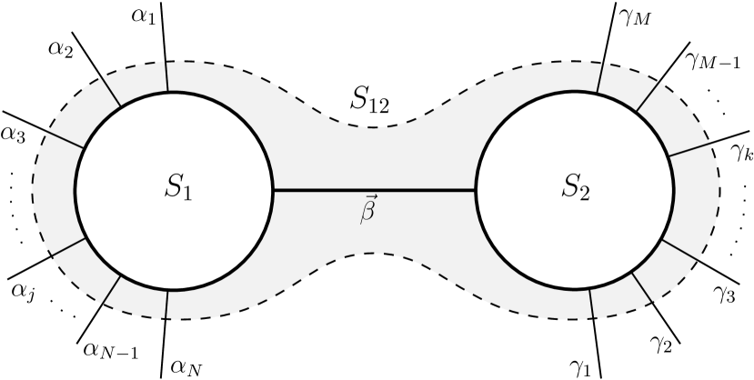
Figure 15: Scheme of two scattering matrices, $S_{1}$ and $S_{2}$, coupled in series, which combine to give $S_{12}$.

Consider two scattering regions $i$=1,2 which are connected in series by one or more internal channels labelled by $\vec{\beta}$, as sketched in Fig. 15. Their respective scattering matrices can be written as

$$\displaystyle{\left(\begin{array}[]{c}\vec{\alpha}^{\prime}\\ \vec{\beta}^{\prime}\\ \end{array}\right)=S_{1}\left(\begin{array}[]{c}\vec{\alpha}\\ \vec{\beta}\\ \end{array}\right)\quad\text{and}\quad\left(\begin{array}[]{c}\vec{\beta}\\ \vec{\gamma}^{\prime}\\ \end{array}\right)=S_{2}\left(\begin{array}[]{c}\vec{\beta}^{\prime}\\ \vec{\gamma}\\ \end{array}\right)}$$ (40)

where the outgoing waves in channels $\vec{\beta}^{\prime}$ of region 1 are ingoing waves of region 2 (and viceversa with $\vec{\beta}$). The scattering matrices are:

$$\displaystyle{S_{i}=\left(\begin{array}[]{cc}r_{i}&t^{\prime}_{i}\\ t_{i}&r^{\prime}_{i}\\ \end{array}\right).}$$ (43)

The scattering matrix of the whole system

$$\displaystyle{\left(\begin{array}[]{c}\vec{\alpha}^{\prime}\\ \vec{\gamma}^{\prime}\\ \end{array}\right)=S_{12}\left(\begin{array}[]{c}\vec{\alpha}\\ \vec{\gamma}\\ \end{array}\right),\quad\text{with}\quad S_{12}=\left(\begin{array}[]{cc}r&t^{\prime}\\ t&r^{\prime}\\ \end{array}\right),}$$ (50)

is obtained by simple linear algebra, leading to

$$r =r_{1}+t^{\prime}_{1}r_{2}(1-r_{1}^{\prime}r_{2})^{-1}t_{1}$$ (51)

$$t =t_{2}(1-r_{1}^{\prime}r_{2})^{-1}t_{1}$$ (52)

$$r^{\prime} =r_{2}^{\prime}+t_{2}(1-r_{1}^{\prime}r_{2})^{-1}r^{\prime}_{1}t^{\prime}_{2}$$ (53)

$$t^{\prime} =t^{\prime}_{1}\left[1+r_{2}(1-r_{1}^{\prime}r_{2})^{-1}r^{\prime}_{1}\right]t^{\prime}_{2}.$$ (54)

In the previous, we have ignored the phases accumulated along the connecting channels. Usually these are the only phases with a physical meaning. A convenient way to take them into account is by taking all arbitrary phases in $S_{1}$ and $S_{2}$ to zero and treating the propagation along the connecting channels as an additional scattering region for which waves are perfectly transmitted along every channel $i$ gaining a phase $\phi_{i}$. For a single channel connection, and in the absence of a magnetic field, this can be written as

$$\displaystyle{S_{\rm ph}(\varphi)=\left(\begin{array}[]{cc}0&e^{i\varphi}\\ e^{i\varphi}&0\\ \end{array}\right).}$$ (57)

In the case of having $N$ channels, we have

$$S_{\rm ph}(\vec{\varphi})=\sum_{i=1}^{N}S_{\rm ph}(\varphi_{i})\otimes{\rm diag}_{N}(\delta_{ii}),$$ (58)

where ${\rm diag}_{N}(\delta_{ii})$ is a $N\times N$ matrix whose only nonvanishing element is the $i$th element of the diagonal, which is 1. The total scattering matrix is hence the result of combining the three matrices $S_{1}$, $S_{\rm ph}(\vec{\varphi})$, and $S_{2}$.

Appendix B Linear coefficients for heat currents

In the linear regime, assuming the probe condition for the tip, $I_{3}=0$, we get for the heat currents

$$J_{i}={\cal M}_{i}(\mu_{2}-\mu_{1})+\sum_{j}{\cal K}_{ij}\delta T_{j},$$ (59)

with ${\cal M}_{1}=-{\cal M}_{2}-{\cal M}_{3}$,

$${\cal M}_{2} =M_{21}+\frac{G_{13}M_{23}}{G_{13}+G_{23}}$$ (60)

$${\cal M}_{3} =\frac{G_{32}M_{31}-G_{13}M_{23}}{G_{13}+G_{23}},$$ (61)

and the thermal conductances:

$${\cal K}_{ij}=q_{\rm H}\delta_{ij}-K_{ij}-\frac{M_{i3}L_{3j}}{G_{31}+G_{32}}.$$ (62)

Appendix C Limitations of the Sommerfeld expansion

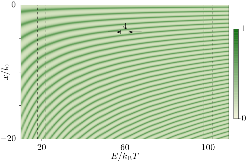
Figure 16: Energy dependence of the transmission probability ${\cal T}_{23}$ as a function of the tip position. The relevant temperature scale $4k_{\text{B}}T$ around the chemical potentials $\mu=20k_{\text{B}}T$ (considered in most figures) and $\mu=100k_{\text{B}}T$ (considered in one of the cases in Fig. 6) is delimited by dashed lines as a guide to the eye.

The Sommerfeld expansion is known to behave well for low temperatures $k_{\text{B}}T\ll\mu$, provided the transmission probabilities are smooth. In our system, the oscillatory energy dependence of the transmission probabilities sets an additional limitation depending on the position of the tip at finite temperatures. The Sommerfeld approximation breaks down when the energy associated to the distance of two peaks,

$$\Delta E=\frac{2\pi^{2}\hbar^{2}}{mx^{2}}\left(1-\frac{1}{\pi}k|x|\right),$$ (63)

becomes comparable to the thermal energy. This depends on the chemical potential around which the current integrals are performed. At short distances, $\Delta E$ diverges, as shown in Fig. 16 for the case of ${\cal T}_{23}$, which stays constant over all energies as $x\rightarrow 0$ (similar behaviour is obtained for ${\cal T}_{12}$ and ${\cal T}_{13}$). $\Delta E$ decreases when the tip separates from the scatterer, most dramatically for low energies.

Appendix D Coupling to a dephasing probe

We obtain the scattering matrix for pure dephasing processes by assuming that the coupling to each of the fictitious probes, $a$ and $b$, is defined by a tunnel barrier with transmission probability $\tau$, cf. Fig. 10(a). The coupling is the same for both probes, so no propagation direction is privileged. We can simply combine the elements of two scattering matrices of the form of Eq. (3), choosing $\phi=0$ in order to avoid the dephasing probe to introduce unnecessary phases. With this, we arrive at

$$\displaystyle{S^{\ocircle}=\left(\begin{array}[]{cccc}0&\sqrt{1{-}\tau}&0&i\sqrt{\tau}\\ \sqrt{1{-}\tau}&0&i\sqrt{\tau}&0\\ i\sqrt{\tau}&0&\sqrt{1{-}\tau}&0\\ 0&i\sqrt{\tau}&0&\sqrt{1{-}\tau}\\ \end{array}\right).}$$ (68)

Note that different conventions are also possible Datta (1995).

We now calculate the transmission probabilities, modified by the presence of the probes, ${\cal T}_{\alpha\beta}^{\pm\tau}$. The indices $\alpha,\beta$ accounting for all conductor terminals (indices $i$ and $j$ will still be used when the probes are explicitly excluded). The transmission probabilities, irrespective of the relative position of the tip, ${\cal T}_{\alpha\beta}^{\tau}$ are obtained from ${\cal T}_{\alpha\beta}^{\pm\tau}$ as it was done in Eq. (11). Note that they do not depend on the position of the probes, but only on how strongly they are coupled to the conductor. In the strongly coupled limit with $\tau=1$, we get ${\cal A}_{\tau}=1$ and $\zeta_{\tau}=0$, i.e. every phase dependence is lost.

Considering that the tip position is $x<0$, the transmission probabilities between the conductor terminals and the tip are modified by the coupling to the pure dephasing probes ($S^{\ocircle}$) with respect to what we got in Eq. (8):

$${\cal T}_{12}^{-\tau} =\frac{(1-R)(1-\tau)(\eta_{+}-\varepsilon)}{2{\cal A}_{\tau}}$$

$${\cal T}_{13}^{-\tau} =\frac{\varepsilon({\cal A}_{\tau}+\zeta_{\tau})}{{\cal A}_{\tau}}$$ (69)

$${\cal T}_{23}^{-\tau} =\frac{(1-R)(1-\tau)\varepsilon}{{\cal A}_{\tau}},$$

where ${\cal A}_{\tau}$ and $\zeta_{\tau}$ are respectively obtained from ${\cal A}$ and $\zeta$ [Eqs. (9) and (10)] by replacing $R\rightarrow R_{\tau}=R(1-\tau)^{2}$. They are now conditioned on the electrons being reflected at the coupling to the probes.

The probabilities for an electron injected from a conductor terminal to be absorbed by one of the probes are:

$${\cal T}_{a1}^{-\tau} =\frac{\tau\eta_{+}^{2}}{4{\cal A}_{\tau}} {\cal T}_{b1}^{-\tau} =(1{-}\tau)R{\cal T}_{a1}^{-\tau}$$

$${\cal T}_{b2}^{-\tau} =\frac{\tau(1-R)}{{\cal A}_{\tau}} {\cal T}_{a2}^{-\tau} =(1{-}\tau)\eta_{-}^{2}{\cal T}_{b2}^{-\tau}/4$$ (70)

$${\cal T}_{a3}^{-\tau} =\frac{\varepsilon\tau}{{\cal A}_{\tau}} {\cal T}_{b3}^{-\tau} =(1{-}\tau)R{\cal T}_{a3}^{-\tau}.$$

For electrons to be transmitted from one probe to the other we find

$${\cal T}_{ab}^{-\tau}=\frac{\tau^{2}\eta_{-}^{2}}{4{\cal A}_{\tau}}\quad{\rm and}\quad{\cal T}_{ba}^{-\tau}=\frac{\tau^{2}R}{{\cal A}_{\tau}}.$$ (71)

By symmetry we obtain the remaining ones: ${\cal T}_{ai}^{-\tau}={\cal T}_{ib}^{-\tau}$ and ${\cal T}_{bi}^{-\tau}={\cal T}_{ia}^{-\tau}$, and, for the internal reflection at the probes: ${\cal T}_{aa}^{-\tau}=1-\sum_{\alpha\neq a}{\cal T}_{a\alpha}^{-\tau}$ and ${\cal T}_{bb}^{-\tau}=1-\sum_{\alpha\neq b}{\cal T}_{b\alpha}^{-\tau}$.

The probabilities ${\cal T}_{\alpha\beta}^{+\tau}$ are obtained from the previous expressions for ${\cal T}_{\alpha\beta}^{-\tau}$, by replacing $1\leftrightarrow 2$ and $a\leftrightarrow b$.

The probe conditions ${\cal I}_{a}(E)={\cal I}_{b}(E)=0$ are satisfied only if the probes acquire a nonequilibrium distribution, in particular

$$f_{\alpha}=\sum_{i}Y_{\alpha i}f_{i},$$ (72)

for terminals $\alpha=a,b$, with $Y_{\alpha i}=y_{\alpha i}/\sum_{i}y_{\alpha i}$ and

$$y_{ai}=(1-{\cal T}_{aa}^{\tau}){\cal T}_{ai}^{\tau}+{\cal T}_{ab}^{\tau}{\cal T}_{bi}^{\tau},$$ (73)

and likely for $y_{bi}$ by replacing $a\leftrightarrow b$. Note that equilibrium properties are recovered as $\sum_{i}Y_{ai}=\sum_{i}Y_{bi}=1$.

The currents in the conductor terminals can then be calculated from

$${\cal I}_{i}=\frac{2e}{h}\sum_{i=1}^{3}\left(\delta_{ij}-\tilde{\cal T}_{ij}\right)f_{i}(E),$$ (74)

with the generalized transmissions:

$$\tilde{\cal T}_{ij}={\cal T}_{ij}^{\tau}+{\cal T}_{ia}^{\tau}Y_{aj}+{\cal T}_{ib}^{\tau}Y_{bj}.$$ (75)

Appendix E Coupling to an invasive probe

Consider that the conductor is coupled to a fictitious probe $p$ via two additional channels, as shown in Fig. 10(b). Imposing that the different channels are not reflected at the probe (i.e., the diagonal elements of the scattering matrix are zero) and that the probe couples symmetrically to the conductor, one finds that the scattering matrix is given by $S_{ij}^{\Diamond}=\sigma_{ij}^{\Diamond}e^{i(\theta_{i}+\theta_{j})}$, with Büttiker (1986)

$$\displaystyle{\sigma^{\Diamond}=\left(\begin{array}[]{cccc}0&\sqrt{1{-}\lambda}&\sqrt{\lambda}&0\\ \sqrt{1{-}\lambda}&0&0&\sqrt{\lambda}\\ \sqrt{\lambda}&0&0&-\sqrt{1{-}\lambda}\\ 0&\sqrt{\lambda}&-\sqrt{1{-}\lambda}&0\\ \end{array}\right),}$$ (80)

where $\lambda$ parametrizes the conductor-probe coupling. Note however that each probe channel is coupled to only one conductor channel, so nothing avoids an electron absorbed by the probe to be reemitted into the same channel, resulting in the reversal of its momentum. For $\lambda=0$, the probe is not coupled. For $\lambda=1$, every electron incoming from the conductor channels are absorbed by the probe. Note that, also in this case, the result does not depend on the position of the probe.

As for the pure dephasing case in Appendix D, we need a four channel scattering matrix (two channels in the conductor and two connected to the probe): a single channel connection (as for the model of the tip) does not include the desired properties that all electrons are absorbed by a strongly coupled probe Büttiker (1986) and that it does not add additional phases to the dynamics.

In this case, the transmission probabilities between conductor terminals ${\cal T}_{ij}^{-\lambda}$ can be obtained from Eqs. (D) by simply replacing $\tau\rightarrow\lambda$. For the new coefficient ${\cal A}_{\lambda}$ one additionally needs to replace $\chi\rightarrow\chi_{\lambda}=\chi+2(\theta_{1}+\theta_{2})$. The transmission probabilities from the probe (considering the contribution of the two channels) are

$${\cal T}_{1p}^{-\lambda} =\frac{\lambda(\eta_{+}-\varepsilon)[1+R{\color[rgb]{.75,0,.25}(1-\lambda)}]}{2{\cal A}_{\lambda}}$$

$${\cal T}_{2p}^{-\lambda} =\frac{\lambda(1-R)[1+(1-\lambda)(\eta_{-}-\varepsilon)]}{{\cal A}_{\lambda}}$$ (81)

$${\cal T}_{3p}^{-\lambda} =\frac{\lambda\varepsilon[1+R{\color[rgb]{.75,0,.25}(1-\lambda)}]}{{\cal A}_{\lambda}}.$$

For the probabilities ${\cal T}_{\alpha\beta}^{+\lambda}$, one needs to exchange 1$\leftrightarrow$2 in the corresponding expressions for ${\cal T}_{\alpha\beta}^{-\lambda}$. Again, all phases are lost for $\lambda=1$.

In this case, the probe maintains the symmetry ${\cal T}_{\alpha\beta}^{\lambda}={\cal T}_{\beta\alpha}^{\lambda}$.

In the case of imposing a quasi-elastic boundary condition ${\cal I}_{p}(E)=0$, as is done in Sec. V.2, we solve for the distribution of the probe, which becomes

$$f_{p}(E)=\frac{{\cal T}_{p1}^{\lambda}f_{1}(E)+{\cal T}_{p2}^{\lambda}f_{2}(E)+{\cal T}_{p3}^{\lambda}f_{3}(E)}{2-{\cal T}_{pp}^{\lambda}},$$ (82)

where the factor 2 in the denominator accounts for the two channels of terminal $p$. The currents at the other conductor terminals $i=1,2,3$ can then be written from

$${\cal I}_{i}=\frac{2}{h}\sum_{j=1}^{3}\left({\cal T}_{ij}^{\lambda}+\frac{{\cal T}_{ip}^{\lambda}{\cal T}_{pj}^{\lambda}}{2-{\cal T}_{pp}^{\lambda}}\right)(f_{i}-f_{j}),$$ (83)

where the second term in the first brackets (proportional to $\lambda$) introduces the transition from the coherent to the incoherent transport regimes Büttiker (1988).

References

- Hicks and Dresselhaus (1993) L. D. Hicks and M. S. Dresselhaus, “Thermoelectric figure of merit of a one-dimensional conductor,” Phys. Rev. B 47, 16631–16634 (1993).
- Mahan and Sofo (1996) G. D. Mahan and J. O. Sofo, “The best thermoelectric,” Proc. Natl. Acad. Sci. USA 93, 7436–7439 (1996).
- Whitney (2014) R. S. Whitney, “Most Efficient Quantum Thermoelectric at Finite Power Output,” Phys. Rev. Lett. 112, 130601 (2014).
- Datta (1995) S. Datta, Electronic Transport in Mesoscopic Systems (Cambridge University Press, 1995).
- Ihn (2009) T. Ihn, Semiconductor Nanostructures: Quantum states and electronic transport (Oxford University Press, 2009).
- Nazarov and Blanter (2009) Y. V. Nazarov and Y. M. Blanter, Quantum Transport: Introduction to Nanoscience (Cambridge University Press, 2009).
- Molenkamp et al. (1990) L. W. Molenkamp, H. van Houten, C. W. J. Beenakker, R. Eppenga, and C. T. Foxon, “Quantum oscillations in the transverse voltage of a channel in the nonlinear transport regime,” Phys. Rev. Lett. 65, 1052–1055 (1990).
- Staring et al. (1993) A. A. M. Staring, L. W. Molenkamp, B. W. Alphenaar, H. van Houten, O. J. A. Buyk, M. A. A. Mabesoone, C. W. J. Beenakker, and C. T. Foxon, “Coulomb-Blockade Oscillations in the Thermopower of a Quantum Dot,” EPL 22, 57–62 (1993).
- Dzurak et al. (1993) A. S. Dzurak, C. G. Smith, M. Pepper, D. A. Ritchie, J. E. F. Frost, G. A. C. Jones, and D. G. Hasko, “Observation of Coulomb blockade oscillations in the thermopower of a quantum dot,” Solid State Commun. 87, 1145–1149 (1993).
- Dzurak et al. (1997) A. S. Dzurak, C. G. Smith, C. H. W. Barnes, M. Pepper, L. Martín-Moreno, C. T. Liang, D. A. Ritchie, and G. A. C. Jones, “Thermoelectric signature of the excitation spectrum of a quantum dot,” Phys. Rev. B 55, R10197–R10200(R) (1997).
- Small et al. (2003) J. P. Small, K. M. Perez, and P. Kim, “Modulation of Thermoelectric Power of Individual Carbon Nanotubes,” Phys. Rev. Lett. 91, 256801 (2003).
- Llaguno et al. (2004) M. C. Llaguno, J. E. Fischer, A. T. Johnson, and J. Hone, “Observation of Thermopower Oscillations in the Coulomb Blockade Regime in a Semiconducting Carbon Nanotube,” Nano Lett. 4, 45–49 (2004).
- Scheibner et al. (2007) R. Scheibner, E. G. Novik, T. Borzenko, M. König, D. Reuter, A. D. Wieck, H. Buhmann, and L. W. Molenkamp, “Sequential and cotunneling behavior in the temperature-dependent thermopower of few-electron quantum dots,” Phys. Rev. B 75, 041301 (2007).
- Svensson et al. (2012) S. F. Svensson, A. I. Persson, E. A. Hoffmann, N. Nakpathomkun, H. A. Nilsson, H. Q. Xu, L. Samuelson, and H. Linke, “Lineshape of the thermopower of quantum dots,” New J. Phys. 14, 033041 (2012).
- Svensson et al. (2013) S. F. Svensson, E. A. Hoffmann, N. Nakpathomkun, P. M. Wu, H. Q. Xu, H. A. Nilsson, D. Sánchez, V. Kashcheyevs, and H. Linke, “Nonlinear thermovoltage and thermocurrent in quantum dots,” New J. Phys. 15, 105011 (2013).
- Thierschmann et al. (2013) H. Thierschmann, M. Henke, J. Knorr, L. Maier, C. Heyn, W. Hansen, H. Buhmann, and L. W. Molenkamp, “Diffusion thermopower of a serial double quantum dot,” New J. Phys. 15, 123010 (2013).
- Harzheim et al. (2020) A. Harzheim, J. K. Sowa, J. L. Swett, G. A. D. Briggs, J. A. Mol, and P. Gehring, “Role of metallic leads and electronic degeneracies in thermoelectric power generation in quantum dots,” Phys. Rev. Res. 2, 013140 (2020).
- Josefsson et al. (2018) M. Josefsson, A. Svilans, A. M. Burke, E. A. Hoffmann, S. Fahlvik, C. Thelander, M. Leijnse, and H. Linke, “A quantum-dot heat engine operating close to the thermodynamic efficiency limits,” Nat. Nanotechnol. 13, 920–924 (2018).
- Finch et al. (2009) C. M. Finch, V. M. García-Suárez, and C. J. Lambert, “Giant thermopower and figure of merit in single-molecule devices,” Phys. Rev. B 79, 033405 (2009).
- Bergfield and Stafford (2009) J. P. Bergfield and C. A. Stafford, “Thermoelectric Signatures of Coherent Transport in Single-Molecule Heterojunctions,” Nano Lett. 9, 3072–3076 (2009).
- Karlström et al. (2011) O. Karlström, H. Linke, G. Karlström, and A. Wacker, “Increasing thermoelectric performance using coherent transport,” Phys. Rev. B 84, 113415 (2011).
- Trocha and Barnaś (2012) P. Trocha and J. Barnaś, “Large enhancement of thermoelectric effects in a double quantum dot system due to interference and Coulomb correlation phenomena,” Phys. Rev. B 85, 085408 (2012).
- Gómez-Silva et al. (2012) G. Gómez-Silva, O. Ávalos Ovando, M. L. Ladrón de Guevara, and P. A. Orellana, “Enhancement of thermoelectric efficiency and violation of the Wiedemann-Franz law due to Fano effect,” J. Appl. Phys. 111, 053704 (2012).
- Hershfield et al. (2013) S. Hershfield, K. A. Muttalib, and B. J. Nartowt, “Nonlinear thermoelectric transport: A class of nanodevices for high efficiency and large power output,” Phys. Rev. B 88, 085426 (2013).
- Benenti et al. (2017) G. Benenti, G. Casati, K. Saito, and R. S. Whitney, “Fundamental aspects of steady-state conversion of heat to work at the nanoscale,” Phys. Rep. 694, 1 (2017).
- Entin-Wohlman et al. (2010) O. Entin-Wohlman, Y. Imry, and A. Aharony, “Three-terminal thermoelectric transport through a molecular junction,” Phys. Rev. B 82, 115314 (2010).
- Sánchez and Büttiker (2011) R. Sánchez and M. Büttiker, “Optimal energy quanta to current conversion,” Phys. Rev. B 83, 085428 (2011).
- Sothmann et al. (2012) B. Sothmann, R. Sánchez, A. N. Jordan, and M. Büttiker, “Rectification of thermal fluctuations in a chaotic cavity heat engine,” Phys. Rev. B 85, 205301 (2012).
- Mazza et al. (2014) F. Mazza, R. Bosisio, G. Benenti, V. Giovannetti, R. Fazio, and F. Taddei, “Thermoelectric efficiency of three-terminal quantum thermal machines,” New J. Phys. 16, 085001 (2014).
- Entin-Wohlman and Aharony (2012) O. Entin-Wohlman and A. Aharony, “Three-terminal thermoelectric transport under broken time-reversal symmetry,” Phys. Rev. B 85, 085401 (2012).
- Sothmann and Büttiker (2012) B. Sothmann and M. Büttiker, “Magnon-driven quantum-dot heat engine,” EPL 99, 27001 (2012).
- Ruokola and Ojanen (2012) T. Ruokola and T. Ojanen, “Theory of single-electron heat engines coupled to electromagnetic environments,” Phys. Rev. B 86, 035454 (2012).
- Jiang et al. (2012) J.-H. Jiang, O. Entin-Wohlman, and Y. Imry, “Thermoelectric three-terminal hopping transport through one-dimensional nanosystems,” Phys. Rev. B 85, 075412 (2012).
- Hofer et al. (2016) P. P. Hofer, J.-R. Souquet, and A. A. Clerk, “Quantum heat engine based on photon-assisted Cooper pair tunneling,” Phys. Rev. B 93, 041418(R) (2016).
- Jordan et al. (2013) A. N. Jordan, B. Sothmann, R. Sánchez, and M. Büttiker, “Powerful and efficient energy harvester with resonant-tunneling quantum dots,” Phys. Rev. B 87, 075312 (2013).
- Bergenfeldt et al. (2014) C. Bergenfeldt, P. Samuelsson, B. Sothmann, C. Flindt, and M. Büttiker, “Hybrid microwave-cavity heat engine,” Phys. Rev. Lett. 112, 076803 (2014).
- Sánchez et al. (2015) R. Sánchez, B. Sothmann, and A. N. Jordan, “Chiral thermoelectrics with quantum Hall edge states,” Phys. Rev. Lett. 114, 146801 (2015).
- Mazza et al. (2015) F. Mazza, S. Valentini, R. Bosisio, G. Benenti, V. Giovannetti, R. Fazio, and F. Taddei, “Separation of heat and charge currents for boosted thermoelectric conversion,” Phys. Rev. B 91, 245435 (2015).
- Bosisio et al. (2016) R. Bosisio, G. Fleury, J.-L. Pichard, and C. Gorini, “Nanowire-based thermoelectric ratchet in the hopping regime,” Phys. Rev. B 93, 165404 (2016).
- Sánchez et al. (2018) R. Sánchez, P. Burset, and A. L. Yeyati, “Cooling by Cooper pair splitting,” Phys. Rev. B 98, 241414 (2018).
- Thierschmann et al. (2015a) H. Thierschmann, R. Sánchez, B. Sothmann, F. Arnold, C. Heyn, W. Hansen, H. Buhmann, and L. W. Molenkamp, “Three-terminal energy harvester with coupled quantum dots,” Nat. Nanotechnol. 10, 854 (2015a).
- Roche et al. (2015) B. Roche, P. Roulleau, T. Jullien, Y. Jompol, I. Farrer, D. A. Ritchie, and D. C. Glattli, “Harvesting dissipated energy with a mesoscopic ratchet,” Nat. Commun. 6, 6738 (2015).
- Jaliel et al. (2019) G. Jaliel, R. K. Puddy, R. Sánchez, A. N. Jordan, B. Sothmann, I. Farrer, J. P. Griffiths, D. A. Ritchie, and C. G. Smith, “Experimental realization of a quantum dot energy harvester,” Phys. Rev. Lett. 123, 117701 (2019).
- Dorsch et al. (2021) S. Dorsch, A. Svilans, M. Josefsson, B. Goldozian, M. Kumar, C. Thelander, A. Wacker, and A. Burke, “Heat Driven Transport in Serial Double Quantum Dot Devices,” Nano Lett. 21, 988–994 (2021).
- Sánchez and Serra (2011) D. Sánchez and L. Serra, “Thermoelectric transport of mesoscopic conductors coupled to voltage and thermal probes,” Phys. Rev. B 84, 201307 (2011).
- Matthews et al. (2012) J. Matthews, D. Sánchez, M. Larsson, and H. Linke, “Thermally driven ballistic rectifier,” Phys. Rev. B 85, 205309 (2012).
- Matthews et al. (2014) J. Matthews, F. Battista, D. Sánchez, P. Samuelsson, and H. Linke, “Experimental verification of reciprocity relations in quantum thermoelectric transport,” Phys. Rev. B 90, 165428 (2014).
- Thierschmann et al. (2015b) H. Thierschmann, F. Arnold, M. Mittermüller, L. Maier, C. Heyn, W. Hansen, H. Buhmann, and L. W. Molenkamp, “Thermal gating of charge currents with Coulomb coupled quantum dots,” New J. Phys. 17, 113003 (2015b).
- Sánchez et al. (2015) R. Sánchez, B. Sothmann, and A. N. Jordan, “Heat diode and engine based on quantum Hall edge states,” New J. Phys. 17, 075006 (2015).
- Jiang et al. (2015) J.-H. Jiang, M. Kulkarni, D. Segal, and Y. Imry, “Phonon thermoelectric transistors and rectifiers,” Phys. Rev. B 92, 045309 (2015).
- Rosselló et al. (2017) G. Rosselló, R. López, and R. Sánchez, “Dynamical Coulomb blockade of thermal transport,” Phys. Rev. B 95, 235404 (2017).
- Sánchez et al. (2017) R. Sánchez, H. Thierschmann, and L. W. Molenkamp, “Single-electron thermal devices coupled to a mesoscopic gate,” New J. Phys. 19, 113040 (2017).
- Hwang et al. (2018) S.-Y. Hwang, F. Giazotto, and B. Sothmann, “Phase-Coherent Heat Circulator Based on Multiterminal Josephson Junctions,” Phys. Rev. Appl. 10, 044062 (2018).
- Goury and Sánchez (2019) D. Goury and R. Sánchez, “Reversible thermal diode and energy harvester with a superconducting quantum interference single-electron transistor,” Appl. Phys. Lett. 115, 092601 (2019).
- Acciai et al. (2021) M. Acciai, F. Hajiloo, F. Hassler, and J. Splettstoesser, “Phase-coherent heat circulators with normal or superconducting contacts,” Phys. Rev. B 103, 085409 (2021).
- Cao et al. (2015) Z. Cao, T.-F. Fang, L. Li, and H.-G. Luo, “Thermoelectric-induced unitary Cooper pair splitting efficiency,” Appl. Phys. Lett. 107, 212601 (2015).
- Machon et al. (2013) P. Machon, M. Eschrig, and W. Belzig, “Nonlocal Thermoelectric Effects and Nonlocal Onsager relations in a Three-Terminal Proximity-Coupled Superconductor-Ferromagnet Device,” Phys. Rev. Lett. 110, 047002 (2013).
- Hussein et al. (2019) R. Hussein, M. Governale, S. Kohler, W. Belzig, F. Giazotto, and A. Braggio, “Nonlocal thermoelectricity in a Cooper-pair splitter,” Phys. Rev. B 99, 075429 (2019).
- Kirsanov et al. (2019) N. S. Kirsanov, Z. B. Tan, D. S. Golubev, P. J. Hakonen, and G. B. Lesovik, “Heat switch and thermoelectric effects based on Cooper-pair splitting and elastic cotunneling,” Phys. Rev. B 99, 115127 (2019).
- Blasi et al. (2020a) G. Blasi, F. Taddei, L. Arrachea, M. Carrega, and A. Braggio, “Nonlocal Thermoelectricity in a Superconductor–Topological-Insulator–Superconductor Junction in Contact with a Normal-Metal Probe: Evidence for Helical Edge States,” Phys. Rev. Lett. 124, 227701 (2020a).
- Blasi et al. (2020b) G. Blasi, F. Taddei, L. Arrachea, M. Carrega, and A. Braggio, “Nonlocal thermoelectricity in a topological Andreev interferometer,” Phys. Rev. B 102, 241302 (2020b).
- Tan et al. (2021) Z. B. Tan, A. Laitinen, N. S. Kirsanov, A. Galda, V. M. Vinokur, M. Haque, A. Savin, D. S. Golubev, G. B. Lesovik, and P. J. Hakonen, “Thermoelectric current in a graphene Cooper pair splitter,” Nat. Commun. 12, 1–7 (2021).
- Binnig and Rohrer (1987) G. Binnig and H. Rohrer, “Scanning tunneling microscopy - from birth to adolescence,” Rev. Mod. Phys. 59, 615 (1987).
- Hasegawa and Avouris (1993) Y. Hasegawa and Ph. Avouris, “Direct observation of standing wave formation at surface steps using scanning tunneling spectroscopy,” Phys. Rev. Lett. 71, 1071–1074 (1993).
- Crommie et al. (1993a) M. F. Crommie, C. P. Lutz, and D. M. Eigler, “Imaging standing waves in a two-dimensional electron gas,” Nature 363, 524–527 (1993a).
- Crommie et al. (1993b) M. F. Crommie, C. P. Lutz, and D. M. Eigler, “Confinement of Electrons to Quantum Corrals on a Metal Surface,” Science 262, 218–220 (1993b).
- Büttiker (1989) M. Büttiker, “Chemical potential oscillations near a barrier in the presence of transport,” Phys. Rev. B 40, 3409–3412(R) (1989).
- Vannucci et al. (2015) L. Vannucci, F. Ronetti, G. Dolcetto, M. Carrega, and M. Sassetti, “Interference-induced thermoelectric switching and heat rectification in quantum Hall junctions,” Phys. Rev. B 92, 075446 (2015).
- Hofer and Sothmann (2015) P. P. Hofer and B. Sothmann, “Quantum heat engines based on electronic Mach-Zehnder interferometers,” Phys. Rev. B 91, 195406 (2015).
- Samuelsson et al. (2017) P. Samuelsson, S. Kheradsoud, and B. Sothmann, “Optimal Quantum Interference Thermoelectric Heat Engine with Edge States,” Phys. Rev. Lett. 118, 256801 (2017).
- Haack and Giazotto (2019) G. Haack and F. Giazotto, “Efficient and tunable Aharonov-Bohm quantum heat engine,” Phys. Rev. B 100, 235442 (2019).
- Marchegiani et al. (2020a) G. Marchegiani, A. Braggio, and F. Giazotto, “Phase-tunable thermoelectricity in a Josephson junction,” Phys. Rev. Res. 2, 043091 (2020a).
- Chen et al. (2012) C. Y. Chen, A. Shik, A. Pitanti, A. Tredicucci, D. Ercolani, L. Sorba, F. Beltram, and H. E. Ruda, “Electron beam induced current in InSb-InAs nanowire type-III heterostructures,” Appl. Phys. Lett. 101, 063116 (2012).
- Harzheim et al. (2018) A. Harzheim, J. Spiece, C. Evangeli, E. McCann, V. Falko, Y. Sheng, J. H. Warner, G. A. D. Briggs, J. A. Mol, P. Gehring, and O. V. Kolosov, “Geometrically Enhanced Thermoelectric Effects in Graphene Nanoconstrictions,” Nano Lett. 18, 7719–7725 (2018).
- Fast et al. (2020) J. Fast, E. Barrigon, M. Kumar, Y. Chen, L. Samuelson, M. Borgström, A. Gustafsson, S. Limpert, A. Burke, and H. Linke, “Hot-carrier separation in heterostructure nanowires observed by electron-beam induced current,” Nanotechnology 31, 394004 (2020).
- Gächter et al. (2020) N. Gächter, F. Könemann, M. Sistani, M. G. Bartmann, M. Sousa, P. Staudinger, A. Lugstein, and B. Gotsmann, “Spatially resolved thermoelectric effects in operando semiconductor–metal nanowire heterostructures,” Nanoscale 12, 20590–20597 (2020).
- Xu et al. (2010) X. Xu, N. M. Gabor, J. S. Alden, A. M. van der Zande, and P. L. McEuen, “Photo-Thermoelectric Effect at a Graphene Interface Junction,” Nano Lett. 10, 562 (2010).
- Lemme et al. (2011) M. C. Lemme, F. H. L. Koppens, A. L. Falk, M. S. Rudner, H. Park, L. S. Levitov, and C. M. Marcus, “Gate-Activated Photoresponse in a Graphene p–n Junction,” Nano Lett. 11, 4134 (2011).
- Zolotavin et al. (2017) P. Zolotavin, C. I. Evans, and D. Natelson, “Substantial local variation of the Seebeck coefficient in gold nanowires,” Nanoscale 9, 9160 (2017).
- Mitra et al. (2021) R. Mitra, M. R. Sahu, A. Sood, T. Taniguchi, K. Watanabe, H. Shtrikman, S. Mukerjee, A. K. Sood, and A. Das, “Anomalous thermopower oscillations in graphene-nanowire vertical heterostructures,” Nanotechnology 32, 345201 (2021).
- Landauer (1988) R. Landauer, “Motion out of noisy states,” J. Stat. Phys. 53, 233–248 (1988).
- Büttiker (1987) M. Büttiker, “Transport as a consequence of state-dependent diffusion,” Z. Phys. B: Condens. Matter 68, 161–167 (1987).
- van Kampen (1988) N. G. van Kampen, “Relative stability in nonuniform temperature,” IBM J. Res. Dev. 32, 107–111 (1988).
- Fleury et al. (2021) G. Fleury, C. Gorini, and R. Sánchez, “Scanning probe-induced thermoelectrics in a quantum point contact,” Appl. Phys. Lett. 119, 043101 (2021).
- Park et al. (2013) J. Park, G. He, R. M. Feenstra, and A.-P. Li, “Atomic-scale mapping of thermoelectric power on graphene: Role of defects and boundaries,” Nano Lett. 13, 3269 (2013).
- Menges et al. (2016) F. Menges, P. Mensch, H. Schmid, H. Riel, A. Stemmer, and B. Gotsmann, “Temperature mapping of operating nanoscale devices by scanning probe thermometry,” Nat. Commun. 7, 10874 (2016).
- Steinacher et al. (2018) R. Steinacher, C. Pöltl, T. Krähenmann, A. Hofmann, C. Reichl, W. Zwerger, W. Wegscheider, R. A. Jalabert, K. Ensslin, D. Weinmann, and T. Ihn, “Scanning gate experiments: From strongly to weakly invasive probes,” Phys. Rev. B 98, 075426 (2018).
- Marguerite et al. (2019) A. Marguerite, J. Birkbeck, A. Aharon-Steinberg, D. Halbertal, K. Bagani, I. Marcus, Y. Myasoedov, A. K. Geim, D. J. Perello, and E. Zeldov, “Imaging work and dissipation in the quantum Hall state in graphene,” Nature 575, 628–633 (2019).
- Sellier et al. (2011) H. Sellier, B. Hackens, P. M. G, F. Martins, S. Baltazar, X. Wallart, L. Desplanque, V. Bayot, and S. Huant, “On the imaging of electron transport in semiconductor quantum structures by scanning-gate microscopy: successes and limitations,” Semicond. Sci. Technol. 26, 064008 (2011).
- Gorini et al. (2013) C. Gorini, R. A. Jalabert, W. Szewc, S. Tomsovic, and D. Weinmann, “Theory of scanning gate microscopy,” Phys. Rev. B 88, 035406 (2013).
- Brun et al. (2019) B. Brun, F. Martins, S. Faniel, A. Cavanna, C. Ulysse, A. Ouerghi, U. Gennser, D. Mailly, P. Simon, S. Huant, M. Sanquer, H. Sellier, V. Bayot, and B. Hackens, “Thermoelectric scanning-gate interferometry on a quantum point contact,” Phys. Rev. Applied 11, 034069 (2019).
- Eom et al. (1998) J. Eom, C.-J. Chien, and V. Chandrasekhar, “Phase Dependent Thermopower in Andreev Interferometers,” Phys. Rev. Lett. 81, 437–440 (1998).
- Parsons et al. (2003) A. Parsons, I. A. Sosnin, and V. T. Petrashov, “Reversal of thermopower oscillations in the mesoscopic Andreev interferometer,” Phys. Rev. B 67, 140502 (2003).
- Jacquod and Whitney (2010) Ph. Jacquod and R. S. Whitney, “Coherent thermoelectric effects in mesoscopic Andreev interferometers,” EPL 91, 67009 (2010).
- Kalenkov and Zaikin (2017) M. S. Kalenkov and A. D. Zaikin, “Large thermoelectric effect in ballistic Andreev interferometers,” Phys. Rev. B 95, 024518 (2017).
- Engquist and Anderson (1981) H.-L. Engquist and P. W. Anderson, “Definition and measurement of the electrical and thermal resistances,” Phys. Rev. B 24, 1151–1154(R) (1981).
- Büttiker (1986) M. Büttiker, “Role of quantum coherence in series resistors,” Phys. Rev. B 33, 3020–3026 (1986).
- Büttiker (1988) M. Büttiker, “Coherent and sequential tunneling in series barriers,” IBM J. Res. Dev. 32, 63–75 (1988).
- de Jong and Beenakker (1996) M. J. M. de Jong and C. W. J. Beenakker, “Semiclassical theory of shot noise in mesoscopic conductors,” Physica A 230, 219–248 (1996).
- Büttiker (1991) M. Büttiker, “Quantum Coherence and Phase Randomization in Series Resistors,” in Resonant Tunneling in Semiconductors (Springer US, Boston, MA, USA, 1991) pp. 213–227.
- Pilgram et al. (2006) S. Pilgram, P. Samuelsson, H. Förster, and M. Büttiker, “Full-Counting Statistics for Voltage and Dephasing Probes,” Phys. Rev. Lett. 97, 066801 (2006).
- Förster et al. (2007) H. Förster, P. Samuelsson, S. Pilgram, and M. Büttiker, “Voltage and dephasing probes in mesoscopic conductors: A study of full-counting statistics,” Phys. Rev. B 75, 035340 (2007).
- Knittel et al. (1999) I. Knittel, F. Gagel, and M. Schreiber, “Quantum transport and momentum-conserving dephasing,” Phys. Rev. B 60, 916–921 (1999).
- Li and Yan (2002) X.-Q. Li and Y. Yan, “Partially coherent tunneling through a series of barriers: Inelastic scattering versus pure dephasing,” Phys. Rev. B 65, 155326 (2002).
- Golizadeh-Mojarad and Datta (2007) R. Golizadeh-Mojarad and S. Datta, “Nonequilibrium Green’s function based models for dephasing in quantum transport,” Phys. Rev. B 75, 081301 (2007).
- Sivan and Imry (1986) U. Sivan and Y. Imry, “Multichannel Landauer formula for thermoelectric transport with application to thermopower near the mobility edge,” Phys. Rev. B 33, 551–558 (1986).
- Streda (1989) P. Streda, “Quantised thermopower of a channel in the ballistic regime,” J. Phys.: Condens. Matter 1, 1025 (1989).
- Butcher (1990) P. N. Butcher, “Thermal and electrical transport formalism for electronic microstructures with many terminals,” J. Phys.: Condens. Matter 2, 4869 (1990).
- van Houten et al. (1992) H. van Houten, L. W. Molenkamp, C. W. J. Beenakker, and C. T. Foxon, “Thermo-electric properties of quantum point contacts,” Semicond. Sci. Technol. 7, B215 (1992).
- Büttiker et al. (1984) M. Büttiker, Y. Imry, and M. Ya. Azbel, “Quantum oscillations in one-dimensional normal-metal rings,” Phys. Rev. A 30, 1982–1989 (1984).
- Gramespacher and Büttiker (1997) T. Gramespacher and M. Büttiker, “Nanoscopic tunneling contacts on mesoscopic multiprobe conductors,” Phys. Rev. B 56, 13026–13034 (1997).
- Gramespacher and Büttiker (1999) T. Gramespacher and M. Büttiker, “Local non-equilibrium distribution of charge carriers in a phase-coherent conductor,” Comptes Rendus de l’Académie des Sciences - Series IIB - Mechanics-Physics-Astronomy 327, 877–884 (1999).
- Whitney (2013) R. S. Whitney, “Nonlinear thermoelectricity in point contacts at pinch off: A catastrophe aids cooling,” Phys. Rev. B 88, 064302 (2013).
- Sánchez and López (2013) D. Sánchez and R. López, “Scattering Theory of Nonlinear Thermoelectric Transport,” Phys. Rev. Lett. 110, 026804 (2013).
- Meair and Jacquod (2013) J. Meair and P. Jacquod, “Scattering theory of nonlinear thermoelectricity in quantum coherent conductors,” J. Phys.: Condens. Matter 25, 082201 (2013).
- Casimir (1945) H. B. G. Casimir, “On Onsager’s Principle of Microscopic Reversibility,” Rev. Mod. Phys. 17, 343–350 (1945).
- Pendry (1983) J. B. Pendry, “Quantum limits to the flow of information and entropy,” J. Phys. A: Math. Gen. 16, 2161–2171 (1983).
- Jacquet and Pillet (2012) Ph. A. Jacquet and C.-A. Pillet, “Temperature and voltage probes far from equilibrium,” Phys. Rev. B 85, 125120 (2012).
- Meair et al. (2014) J. Meair, J. P. Bergfield, C. A. Stafford, and Ph. Jacquod, “Local temperature of out-of-equilibrium quantum electron systems,” Phys. Rev. B 90, 035407 (2014).
- Argüello-Luengo et al. (2015) J. Argüello-Luengo, D. Sánchez, and R. López, “Heat asymmetries in nanoscale conductors: The role of decoherence and inelasticity,” Phys. Rev. B 91, 165431 (2015).
- Stafford (2016) C. A. Stafford, “Local temperature of an interacting quantum system far from equilibrium,” Phys. Rev. B 93, 245403 (2016).
- Tikhonov et al. (2020) E. S. Tikhonov, A. O. Denisov, S. U. Piatrusha, I. N. Khrapach, J. P. Pekola, B. Karimi, R. N. Jabdaraghi, and V. S. Khrapai, “Spatial and energy resolution of electronic states by shot noise,” Phys. Rev. B 102, 085417 (2020).
- Halbertal et al. (2016) D. Halbertal, J. Cuppens, M. B. Shalom, L. Embon, N. Shadmi, Y. Anahory, H. R. Naren, J. Sarkar, A. Uri, Y. Ronen, Y. Myasoedov, L. S. Levitov, E. Joselevich, A. K. Geim, and E. Zeldov, “Nanoscale thermal imaging of dissipation in quantum systems,” Nature 539, 407–410 (2016).
- Halbertal et al. (2017) D. Halbertal, M. Ben Shalom, A. Uri, K. Bagani, A. Y. Meltzer, I. Marcus, Y. Myasoedov, J. Birkbeck, L. S. Levitov, A. K. Geim, and E. Zeldov, “Imaging resonant dissipation from individual atomic defects in graphene,” Science 358, 1303–1306 (2017).
- Zhang et al. (2019) D. Zhang, X. Zheng, and M. Di Ventra, “Local temperatures out of equilibrium,” Phys. Rep. 830, 1–66 (2019).
- (126) We have already discussed how a spatially resolved measurement (the one made by the tip) introduces privileged phases resulting in thermoelectric contributions. The thermometer does not yield any such contributions, precisely since it lacks resolution.
- Humphrey et al. (2002) T. E. Humphrey, R. Newbury, R. P. Taylor, and H. Linke, “Reversible quantum Brownian heat engines for electrons,” Phys. Rev. Lett. 89, 116801 (2002).
- Paulsson and Datta (2003) M. Paulsson and S. Datta, “Thermoelectric effect in molecular electronics,” Phys. Rev. B 67, 241403 (2003).
- Nakpathomkun et al. (2010) N. Nakpathomkun, H. Q. Xu, and H. Linke, “Thermoelectric efficiency at maximum power in low-dimensional systems,” Phys. Rev. B 82, 235428 (2010).
- Cui et al. (2017) L. Cui, R. Miao, K. Wang, D. Thompson, L. A. Zotti, J. C. Cuevas, E. Meyhofer, and P. Reddy, “Peltier cooling in molecular junctions,” Nat. Nanotechnol. 13, 122–127 (2017).
- Blanter et al. (1998) Ya. M. Blanter, F. W. J. Hekking, and M. Büttiker, “Interaction Constants and Dynamic Conductance of a Gated Wire,” Phys. Rev. Lett. 81, 1925–1928 (1998).
- Imura et al. (2002) K.-I. Imura, K.-V. Pham, P. Lederer, and F. Piéchon, “Conductance of one-dimensional quantum wires,” Phys. Rev. B 66, 035313 (2002).
- Crépieux et al. (2003) A. Crépieux, R. Guyon, P. Devillard, and T. Martin, “Electron injection in a nanotube: Noise correlations and entanglement,” Phys. Rev. B 67, 205408 (2003).
- Guigou et al. (2009a) M. Guigou, T. Martin, and A. Crépieux, “Screening of a Luttinger liquid wire by a scanning tunneling microscope tip. I. Spectral properties,” Phys. Rev. B 80, 045420 (2009a).
- Guigou et al. (2009b) M. Guigou, T. Martin, and A. Crépieux, “Screening of a Luttinger liquid wire by a scanning tunneling microscope tip. II. Transport properties,” Phys. Rev. B 80, 045421 (2009b).
- Marchegiani et al. (2020b) G. Marchegiani, A. Braggio, and F. Giazotto, “Nonlinear thermoelectricity with electron-hole symmetric systems,” Phys. Rev. Lett. 124, 106801 (2020b).