Empirical Evaluation of Circuit Approximations on Noisy Quantum Devices

Abstract.

Noisy Intermediate-Scale Quantum (NISQ) devices fail to produce outputs with sufficient fidelity for deep circuits with many gates today. Such devices suffer from read-out, multi-qubit gate and cross-talk noise combined with short decoherence times limiting circuit depth. This work develops a methodology to generate shorter circuits with fewer multi-qubit gates whose unitary transformations approximate the original reference one. It explores the benefit of such generated approximations under NISQ devices. Experimental results with Grover’s algorithm, multiple-control Toffoli gates, and the Transverse Field Ising Model show that such approximate circuits produce higher fidelity results than longer, theoretically precise circuits on NISQ devices, especially when the reference circuits have many CNOT gates to begin with. With this ability to fine-tune circuits, it is demonstrated that quantum computations can be performed for more complex problems on today’s devices than was feasible before, sometimes even with a gain in overall precision by up to 60%.

1. Introduction

Contemporary quantum computing devices are commonly referred to as Noisy Intermediate-Scale Quantum (NISQ) computers as they are fraught by a multitude of device, systemic, and environmental sources of noise that adversely affect results of computations (preskill2018, ). A number of factors contribute to noise, or errors, experienced during the execution of a quantum program. These include

• noise related to limits on qubit excitation time and program runtime due to decoherence;

• noise related to operations, i.e., gates performing transformations on the states of one or more qubits;

• noise related to interference from (crosstalk with) other qubits; and

• noise subject to the process of measuring the state of a qubit via a detector when producing a program’s output.

Efforts to reduce — or otherwise mitigate — noise are at the front of the effort to create better, more practical quantum computers today (Murali2019, ; murali2019noise, ; wilson20, ; scaffcc, ; preskill2018, ; ibm-pulses, ; openpulse, ; zulehner2018efficient, ; DBLP:conf/micro/TannuQ19, ; DBLP:conf/micro/TannuQ19a, ; Tannu:2019:QCE:3297858.3304007, ; li2019tackling, ; liquantum2020, ; wille2016look, ; siraichi2018qubit, ). Our work builds upon and complements these previous efforts.

All of these sources of noise have a common characteristic in that noise becomes worse with circuit depth, i.e., the more sequential gates a quantum circuit has, as quantum states (particularly excited states) decohere over time. Today’s NISQ devices feature qubits with relatively short coherence times — the longer an excited state has to be maintained, the more noise is introduced, to the point where eventually noise dominates and the original state become unrecoverable. Current devices also suffer from noisy or imprecise gates, which add imprecision to a circuit each time a gate is applied, i.e., qubit state diverges slightly from the expected state with the application of each transformation (rotation). Depending on the type of gate, noise varies significantly: Gates operating on two qubits are an order of magnitude more noisy than single qubit gates. Two qubit gates also experience more cross-talk, due to interference with other qubits in close vicinity. Finally, measurement of state (read-outs) is also subject to considerable noise, on par with cross talk and two qubit gates, as opposed to said single qubit noise.

A quantum program expressed as a circuit of gates operating on virtual qubits needs to be translated into a sequence of pulses directed at physical qubits. This translation step (a.k.a. transpilation) offers optimization opportunities to reduce noise. Besides translation of pulses, quantum compilers consider secondary, noise-related objectives to generate optimized quantum programs, e.g., by mapping virtual qubits to less noisy physical qubits (in terms of readouts) (murali2019noise, ; Tannu:2019:QCE:3297858.3304007, ; DBLP:conf/micro/TannuQ19, ) and their connections (for two qubit gates) (murali2019noise, ; DBLP:conf/micro/TannuQ19a, ), or even by increasing the distance to reduce cross-talk between qubits for a given device layout (ibm-pulses, ; murali20, ; ding20, ).

Another angle to address noise is to reduce the depth of circuits. By reducing the number of gates in a circuit, especially the number of two-qubit gates, the depth of the circuit, i.e., the span of time during which qubits remain in excited states, is shortened, which lowers the effect of decoherence. In fact, this may well bring long circuits within reach of short decoherence times that otherwise could not finish on a NISQ device before losing their states. One promising way to reduce the number of gates is to create an approximate circuit (Amy2013, ; DeVos2015, ; alam20, ), i.e., a circuit which does not provide an exact (theoretically perfect) transformation for a target unitary but rather a “close” fit for the unitary. (One could make a comparison to fixed precision arithmetic in classical computation here, which often relies on converging calculations as an approximation of exact numerical results.) On a NISQ device, an exact quantum circuit is prone to develop large error with increasing circuit depth. In contrast, a near-equivalent approximate quantum circuit with shorter depth, even though subject to a slightly incorrect transformation, may have the potential to yield a result that is closer to the noise-free (theoretically) desired output. This opens up an interesting trade-off between longer-depth theoretical precision with more noise vs. shorter-depth approximation with less noise. It is this trade-off this work aims to assess and quantify.

The task of finding an approximate circuit is similar to the process of circuit synthesis (qs, ; qfast, ). Circuit synthesis is another avenue that attempts to reduce circuit depth. Synthesis here refers to the process of what can be considered design space exploration: Given a quantum program, expressed as an exact circuit or an equivalent unitary matrix, other circuits are systematically constructed and then evaluated in a search for an equivalent, shorter depth quantum circuit with the same unitary. If found, such a target circuit can be transpiled to a specific machine layout and set of gates with shorter execution time, which may be within the given decoherence threshold of a NISQ device.

The main difference between circuit synthesis and searching for an approximate circuit is that instead of searching for an equivalent (functionally indistinguishable) circuit, the latter searches for an approximate circuit of a shorter depth with a slightly different unitary. While this leads to inferior results on a noise-free machine, the intuition is that due to noisy gates, shorter, approximate circuits have the potential to outperform longer, more precise circuits.

There are many different metrics which can be used to determine whether two circuits are equivalent. Quantum synthesis compilers (qs, ; qfast, ) typically use distance metrics between “process” representations of the program, such as the Hilbert-Schmidt (HS) distance between the associated unitary matrices, or the diamond norm (Gilchrist_2005, ; ahar97, ). In the process view, two programs are deemed equivalent when at distance “zero”.

In the context of this work aiming at approximation, synthesis is used to find a circuit exceeding a distance of zero relative to the original program so that, when run on a NISQ machine, its output is expected to be close to that of the original program. One challenge with using approximate circuits is that of finding a suitable metric to assess the appropriateness of a set of approximate circuits. One potential option is a process distance, such as HS, within a certain range (threshold). Another is to instead consider output-related metrics, such as the Jensen-Shannon Divergence or Total Variation Distance (endres_03, ). This remains an open question.

The novelty of this work is in its focus on the analysis of a particular use-case of approximate circuits, namely by considering a set of approximate circuits created by quantum synthesis software. When these offered an unworkable number of circuits, we constrained which ones we used by a given HS distance as a threshold. We never choose an HS threshold of less than 0.1, which still results in a wide range of approximate circuits. With a large selection of circuits we can investigate the behavior of many approximate circuits in the presence of different noise levels.

With this work, we make the following novel contributions to the broader aim of searching for approximate circuits:

• We demonstrate how to obtain a wide range of approximate circuits from custom modified circuit synthesis tools.

• We provide a proof-of-concept that approximate circuits can outperform exact circuits on NISQ devices for small, well known algorithms — Grover’s Algorithm and the Multiple-control Toffoli gate — as well as a specific physics application, namely the three-four qubit Transverse Field Ising Model (TFIM).

• We show how the results of approximate circuits change relative to the noise induced by two-qubit errors. Specifically, we assess the effect of two-qubit errors of lower-depth circuits with different approximation thresholds vs. that of the exact, longer circuit. Experiments indicate improvements in overall precision for shorter approximate circuits over longer precise ones by up to 60%.

2. Problem Statement and Objectives

This work seeks to assess if approximate circuits can outperform exact circuits on today’s NISQ devices. Utilizing approximate circuits ultimately comes with challenges posing four fundamental questions:

1. How can approximate circuits be generated?

2. Can the search for or generation process of approximate circuits be constrained and, if so, how?

3. Will the resulting approximate circuits outperform their equivalent original ones?

4. Can algorithms be designed to make circuit synthesis and the search of resulting circuits scalable?

Before investigating these problems, however, a more fundamental question should be asked: Is there any value in approximate circuits to begin with? In other words, can any approximate circuit actually outperform the original circuit at all? It is this line of reasoning that our work is trying to answer — before we can explore the more general challenges posed by the four questions above.

In this work, we show that there is potential value in approximate circuits: They can outperform theoretically perfect circuits on today’s NISQ hardware. We also confirm that any method of selecting appropriate approximate circuits will need to take the noise/error levels of target devices into account.

3. Design

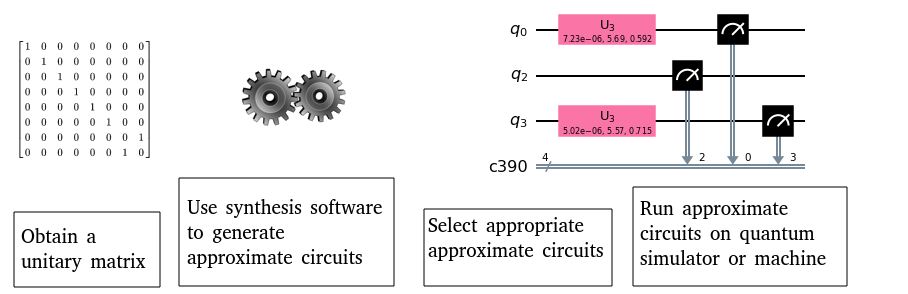
Figure 1. Generic workflow of using approximate circuits. The example is an approximation of the first timestep of the TFIM circuit.

One way to find approximate circuits is to look at approximate circuits generated by the intermediate steps of circuit synthesis programs. These programs do not typically scale to a level which would make them an ideal way to create large approximate circuits in practice, but are an easy way to create them as a proof of concept. Synthesis programs typically look for the shortest circuit they can find with a distance of some kind at “zero”. As these programs are interested in finding as short a circuit as possible, they tend to investigate many shorter circuits before finding their target; these circuits are already nearly optimized for their layout, making them ideal approximate candidates.

Before utilizing synthesis software to generate approximate circuits, we typically need to alter the synthesis tools to produce as output, besides a single circuit, additional circuits that are farther away from the target. These tools already generate and test many circuits during the search for an equivalent circuit, which allows our enhancements to integrate naturally with the existing flow within synthesis tools.

Figure 1 shows the workflow of our process. We first need to obtain our target unitary. Quantum operations can be represented by matrices, and the target unitary is the result of multiplying these transforming matrices of a circuit (or subcircuit) that is to be approximated. In IBM’s Qiskit python interface (Qiskit, ), the unitary of a circuit can be obtained with the following command on the target QuantumCircuit object $circuit$:

$$matrix=qiskit.quantum\_info.Operator(circuit).data$$

The second step is to use our altered synthesis software to generate approximate circuits for our target matrix.

Third, given the the enhanced synthesis software that outputs every circuit it checks, we need to select which approximate circuits we want to check. How to perform this selection is still an open question. For our analysis, we intend to compare a large number of circuits, so we select many circuits with little to no filter for pre-selecting the most accurate ones.

Finally, the selected circuits need to be run on a quantum machine or simulator. For our study, we then compare the results with the expected output, either a known value or our original circuit run on a simulator with no errors.

4. Implementation

For our exploration of approximate circuits, we use two different synthesis tools, QSearch and QFast, both of which are part of the Berkeley Quantum Synthesis Toolkit (BQSkit).

The QSearch (qs, ) optimal depth circuit synthesis tool builds a sequence of circuits of increasing length and decreasing HS distance until it finds the first circuit with a distance of “zero”, a value which can be specified but which defaults to less than 1e-10. It does this by following the A* algorithm. Specifically, it explores different branches of the circuit space by adding on blocks of three gates. Certain machine layouts can be taken into account by restricting these blocks to only being placed between connected qubits. These blocks are made up of one two qubit controlled NOT (CNOT) gate and two single qubit U3 gates on each of the same qubits. The U3 parameters are optimized using one of a number of different numerical optimizers, including COBYLA and BFGS, provided by SciPy 1.20, and reoptimized after each step. This optimization ensures that, for this specific layout of CNOT and U3 gates, this circuit is the closest possible to the target. Because it considers each option, this is guaranteed to be depth optimal with respect to two-qubit gates.

The QFast (qfast, ) synthesis tool likewise builds a sequence of circuits of increasing length, but it has a more complicated algorithm for finding circuits of increasingly higher quality. QFast is not guaranteed to be optimal and gives less of a choice of approximate circuits, but handles circuits with more qubits than QSearch within acceptable search times.

In our work we enhance the QSearch software such that instead of saving only the final circuit, it also saves every intermediate circuit during its search. We then select a portion of the circuits, always with a maximum HS distance threshold of at least 0.1, in order to have a wide range of circuits but none which differ entirely from the target circuit. QFast requires no source code alteration, but it needs to be given a dictionary with the key of “partial_solution_callback” pointing to a function to output these solutions. This dictionary is used by calling QFast with the keyword “model_options”.

These circuits are then executed in three different methods. First, they are executed on the IBM Qiskit (ibm-noise-sim, ) simulator using hardware specific (ibmq_ourense, ibmq_toronto, ibmq_manhattan, ibmq_rome, ibmq_santiago) noise models. These noise models are created using error data collected from IBM’s own physical machines, creating a noisy simulator.

Second, they are executed on noise level sweeps. These use the ibmq_ourense noise model as a base, but change the two-qubit gate noise level during a sensitivity study in order to observe the effect of different types and levels of noise.

Finally, The approximate circuits are also executed on the ibmq_ manhattan, ibmq_toronto, and ibmq_rome physical machines.

5. Experimental Framework

We selected three different algorithms for the evaluation. We start with circuits generated (bassman2020towards, ; bassman2021constantdepth, ) for the time-dependent Transverse Field Ising Model (TFIM). The TFIM is a quintessential model for studying various condensed matter systems, and its time-dependent manifestation shows promise for revealing new information about non-equilibrium effects in materials. Current algorithms for designing quantum circuits for the simulation of such models, however, produce circuits that increase in depth with the growing number of time-steps; circuits quickly grow beyond the NISQ fidelity budget, placing tight limits on the number of time-steps that can be simulated. This class of circuits, therefore, stands to greatly benefit from shorter, approximate circuits. In addition, the output for these circuits can be condensed to a single number to easily be compared to the output of the approximate circuits, allowing for an easy target for the approximate circuits.

We next study Grover’s algorithm (Grover1996:search, ) followed by the multi-control Toffoli gate (Toffoli_1980, ) to demonstrate the general capability of our method.

We decided to focus on small circuits for this work due to NISQ and synthesis limitations. We use the three and four qubit execution of the circuits for most of our experiments, and scale up to five qubits with the multi-control Toffoli gate. For TFIM, we assess at the first 21 time steps of 3ns. This results in 21 different circuits for different times in the evolution of the magnetization. All of these circuits are related, but they can also be investigated individually.

IBM Machine	Num. qubits	Av. CNOT err.
Manhattan	65	.01578
Toronto	27	.01377
Santiago	5	.01131
Rome	5	.02965
Ourense	5	.00767

Table 1. Average CNOT errors on a selection of IBM physical machines as of 2021/01/18

Table 1 provides a snapshot of typical CNOT error rates at the time of writing. they give a contemporary view of the types of CNOT errors that we compare against and reflect the constant changes of NISQ devices with different error rates on different qubit connections even on the same device.

For our experiments using simulators we transpile under IBM’s optimization level 1 with mappings to qubits 0, 1, 2, 3, and 4. Our experiments on physical machines are transpiled under optimization level 3, which at the time of writing allows IBM to map virtual qubits to the best available physical qubits. All work is performed with Python 3.8.2 and Qiskit 0.18.3, Qiskit-aer 0.5.1, Qiskit-ibmq-provider 0.6.1, and Qiskit-terra 0.13.0. Our QSearch enhancements are based on search_compiler version 1.2.1, and we used QFast version 2.1.0.

6. Results

We first report experimental results for simulations under given noise models of contemporary quantum devices subject to NISQ constraints. We then perform a sensitivity study on the effect of noise levels, including both smaller (future) and larger (past) noise levels than seen on the reference device, still using simulation. This is followed by experiments on IBM Q devices with approximate circuits under default transpilation with full optimization. Finally, we perform a sensitivity study investigating the effect of how approximate circuits are mapped to qubits on hardware devices with respect to noise level, particularly of CNOT gates.

6.1. Noise Model Simulations

We first investigate the noise and approximation quality of our approach. Figure 2 depicts results for a 3-qubit TFIM problem under the Toronto (IBM Q) noise model with magnetization (y-axis) over time steps (x-axis) in 21 intervals of 3ns each. Series “Noise free reference” shows the result for the circuit generated by the TFIM domain generator and simulated on the ideal hardware. This is the target for the other circuits; the closer they are to these results, the better they are. Series “Noisy reference” shows the behavior of the same circuits when simulated with the hardware specific noise model. “Noisy reference” behavior quickly diverges from the ideal as circuits become more complex with increasing timesteps. Series “Minimal HS” shows the behavior of the synthesized circuits when using process metrics (HS) as the quality indicator. As these are much shorter (six CNOTs versus tens of CNOTs for the reference circuit) than the baseline implementation, their results are typically closer to the ideal results.

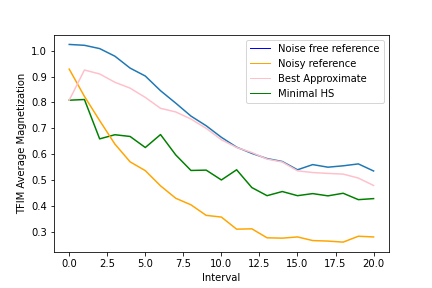
Figure 2. Magnetization over 21 timesteps of selected (best/minimal HS) approximate circuits for the 3-qubit TFIM using the Toronto error model.

The potential of approximate circuits is depicted by Series “Best approximate”, where we select the circuits with “best” output behavior. Their CNOT depth is always shorter than the HS=0 circuits, and so even though the process distance is greater they provide a result closer to the noise free reference. This was also observed across other noise models.

Observation 1: Short approximate circuits can outperform long circuits with a lower process distance in simulation under device noise models.

Let us investigate the range of solutions generated by approximate circuits in more detail. Figure  3 shares the noise free and noisy reference data series with Figure 2, but it additionally includes dots representing each approximate circuit. The colors of the dots indicate how many CNOTs were used in the approximate circuits; in this case, red dots represent two CNOTs and blue dots represent six. It can be seen that while there was a wide difference in accuracy over the different approximate circuits, nearly all of them performed better than the noisy reference.

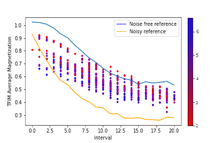
Figure 3. Magnetization over 21 timesteps of all approximate circuits for the 3-qubit TFIM using the Toronto error model.

We next investigate the impact of circuit width (in qubits) and depth (in CNOT gates) for the same TFIM application. Figure 4 represents the four qubit TFIM circuit with the same line graphs again. The number of CNOTs in an individual circuit in this case can range from 1 to 48, which illustrates the wide range of approximate circuits, many of which are closer to the noiseless reference than the noisy reference is.

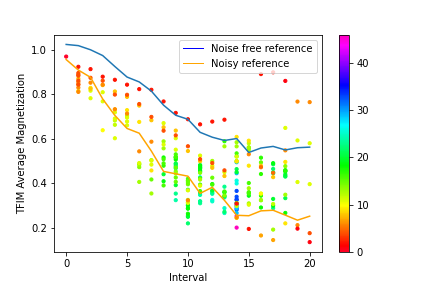
Figure 4. Magnetization over 21 timesteps of approximate circuits for 4 qubit TFIM sing the Santiago noise model.

We now turn our investigation to the impact of circuit approximation for different algorithms and circuits, first with Grover and then with Toffoli. Figure 5 depicts results for Grover’s algorithm with a search target of ’111’ over eight boxes, where each dot represents a circuit. The blue dots each indicate an approximate circuit, while the orange dot and the line represent the output circuit of the hand-coded reference implementation with nine CNOTs. Figure 5 shows the quality of the circuits as the probability of selecting the correct box (y-axis), where higher probability is better. Here, CNOT count is shown on the x-axis rather than indicated by color coding. This shows a wide array of approximate circuits, many of which outperform the reference; only a smaller fraction (below the dashed line) underperform. The challenge here is to select a “good” approximate circuit from the wide array of possible candidates. We observe and investigate this challenge with different metrics but its solution is ultimately beyond the scope of this paper.

Observation 2: To capitalize on the potential of approximate circuits, a selection method and an associate metric are required to ensure superior performance under noise.

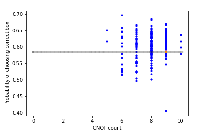
Figure 5. Probability of correct result over CNOT count of approximate circuits for 3 qubit Grover’s algorithm using the Toronto noise model. Reference circuit in red.

We further perform experiments for the Toffoli gate with different numbers of qubits. Figure 6 shows the results for four qubit Toffoli gate—that is, three control qubits to one target qubit. We use the Jensen Shannon (JS) distance(endres_03, ) to analyze these circuits (y-axis), as the Toffoli gate can be programmed to represent a variety of functions, each with different (but known) output. We test each approximate circuits for a subset of such functions and parameters since a given circuit results in different probabilities for correct output. The JS distance provides a composite metric to reflect accuracy (lower is better in this case).

The four qubit results indicate that low-depth approximate circuits outperform those with high CNOT depth. The orange dot on the dashed line represents Qiskit’s multiple-control Toffoli gate without any ancilla bits while the red dot indicates QFast’s default result of an equivalent circuit. The JS metric indicates that the former (orange) outperforms the latter (red). Furthermore, many deeper approximate circuits perform worse than Qiskit’s Toffoli without ancilla while shorter approximations (below the line) can provide even better results than Qiskit. This implies that there is room for improvement even over the reference implementation of given circuits on today’s noisy machines.

Observation 3: Approximate circuits generated from synthesis can outperform discrete reference circuits under noise.

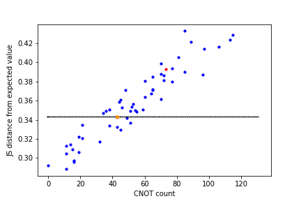
Figure 6. Jensen Shannon (JS) distance over CNOT count of approximate circuits for 4 qubit Toffoli compared to the reference circuit using the Manhattan noise model. Qiskit (orange) and QFast (red) circuits are outperformed by other approximate circuits.

Figure 7 depicts results for a five qubit Toffoli gate, again without any ancilla qubits for either the reference or approximate circuits. These results reinforce the earlier four qubit results: The JS distance of the reference circuit is higher for five qubits, but some approximate circuits have a distance even closer to zero than the best of those for the four qubit Toffoli gate. The correlation of shorter circuits performing better is evident, but outliers exist. As the number of CNOTs increases to the hundreds, the JS values approach 0.465. This is significant because, in this implementation, random noise (an equal number of results of 00000 as 00001 as 00010 and so on) results in a JS distance from the target of 0.465.

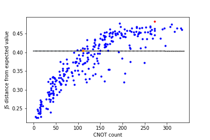
Figure 7. JS distance over CNOT count of approximate circuits for 5 qubit Toffoli compared to the reference circuit using the Manhattan noise model.

We also performed experiments for a 3-qubit Toffoli gate. In this case, the 3-qubit approximate circuits performed poorly compared to the optimized hand-crafted Toffoli gate commonly used, which uses only 6 CNOTs (graph omitted). This illustrates that simple, short circuits provide little benefit for approximations via QSearch or QFast whereas deeper and more complex ones can benefit significantly for today’s noisy quantum hardware. It also presents a challenge for synthesis tools as wider circuits (beyond 6-8 qubits) with corresponding depth results in excessive search cost.

Observation 4: The benefit of using approximate circuits increases with the depth of the reference circuit.

6.2. Error Sensitivity Studies

We assess the sensitivity of approximate circuits to noise. To this end, we use the Ourense noise model as a base but change the CNOT error rate to assess how the performance of circuits changes results in response. Figures 8, 9, and 10 present the approximate circuits with increasing noise. Circuits are again color coded using their depth, with red circuits consisting of two CNOTs and blue circuits of six. The lines of these colors represent the best performing approximate circuits for that number of CNOT gates.

Figure 8 depicts simulations for a CNOT noise level of zero. It illustrates the spread of circuits with different noise sources (with the exception of CNOT noise), and shows that CNOT depth is not closely correlated to the quality of results with no CNOT noise.

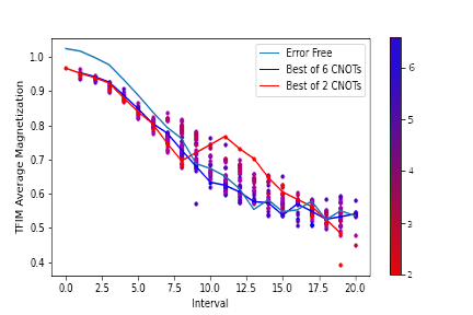
Figure 8. Magnetization over 21 timesteps of approximate circuits for 3-qubit TFIM using the Ourense noise model with no CNOT error.

Figure 9 shows the simulation for a CNOT error of 0.12, similar to that of today’s lowest quality physical devices, and assesses the impact on performance. Note that the increase in CNOT error is accompanied by a decrease in the observed average magnetization. Many of the longer circuits in blue or purple, which were covered up by the red dots, become visible showing that a diverse number of approximate circuits react differently under CNOT noise.

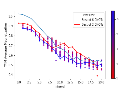
Figure 9. Magnetization over 21 timesteps of approximate circuits for 3-qubit TFIM using the Ourense noise model with a simulated CNOT error of 0.12.

Figure 10 depicts simulations for a CNOT error of 0.24, which is worse than many current IBM machines and reinforces this trend. These results are promising. We clearly see that some individual circuits improve, i.e., more closely approximate the error free reference, with an increase in two-qubit error. We also see that deeper circuits are more affected by CNOT error than shallower circuits. With a low two-qubit error, many of the deeper circuits lie on the line corresponding to the error free reference. As this error increases, these deep circuits quickly decline in quality, and the shallower circuits perform relatively better. This is seen as the best of the longest circuits perform worse than the best of the shortest circuits for all timesteps; but without CNOT noise, this is not necessarily true. Some of these circuits actually benefit from the noise and more closely approximate the error free reference.

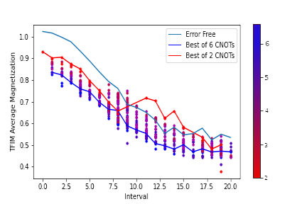
Figure 10. Magnetization over 21 timesteps of approximate circuits for 3-qubit TFIM using the Ourense noise model with a simulated CNOT error of 0.24.

The takeaway from this trend is that different approximate circuits should be chosen based on the error levels of the physical machine. A program can afford to use a long circuit on machines with low error, but a noisier machine will benefit from a shorter, approximate circuit.

Observation 5: Beyond merely being less affected by noise than the reference circuit, some approximate circuits perform better in the presence of noise. This performance increase is dependent on the noise parameters of the system.

Figure 11 further supports this by depicting the depth of the best performing circuit for different noise levels. A trend can be seen: the worse the error (the more red the line), the shallower the circuits with the highest performance in general, but not under all circumstances. A similar trend is seen with our other algorithms (figures omitted).

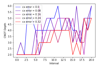
Figure 11. CNOT depth over 21 timesteps of approximate circuits for TFIM showing the best approximate circuits for select CNOT errors.

These results generally support the initial conjecture: as the amount of noise in the models increases, the output quality of deeper circuits deteriorates more quickly than that of the shallower circuits. This causes some of the shallower circuits to produce results that are closer to the ideal results than the deeper circuits, even though the deeper circuits would perform better on an ideal, noise-free machine. This is most noticeable with circuits that contain many CNOTs and on noisier models. It is less noticeable with circuits which are already short or simulated on models of low noise.

Observation 6: The greater the level of two-qubit noise on the target machine, the more benefit is gained from short approximate circuits.

6.3. Results on IBM Q Hardware

Figures 12 and 13 depict results from running the three and four qubit TFIM circuits on contemporary IBM quantum hardware devices. These results provide insight on how much can be gained from using approximate circuits in practice today. We observe that almost all of the approximate circuits in Figure 12 and the large majority of the approximate circuits in Figure 13 perform better than the default circuits.

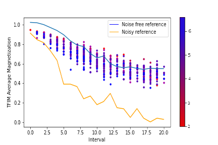
Figure 12. Magnetization over 21 intervals of approximate circuits for 3 qubit TFIM on the Manhattan physical machine.

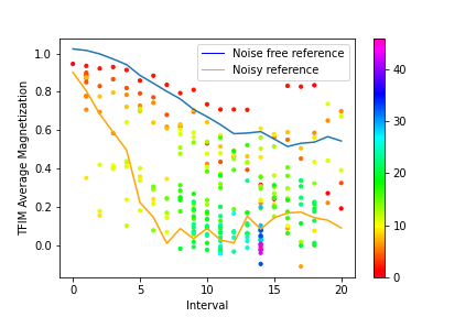
Figure 13. Magnetization over 21 timesteps of approximate circuits for 4 qubit TFIM on the Manhattan physical machine.

We also observe that the approximate circuits here are distributed similarly to Figure 9, showing that the earlier constructed noise models are not far off from actual noise on hardware today.

Observation 7: Approximate circuits can perform well compared to reference circuits on real quantum hardware devices as well as on noisy simulators.

Figure 14, similar to Figure 5, depicts results from experiments with the 3 qubit implementation of Grover’s algorithm. As before, many (but not all) of the approximate circuits perform better than the reference circuit. There is a minor bias to shorter circuits performing better, but not a significant one. It should be noted that the reference circuit here had more than 50 CNOTs and is thus omitted from the figure. The line is still at the performance level of the reference circuit.

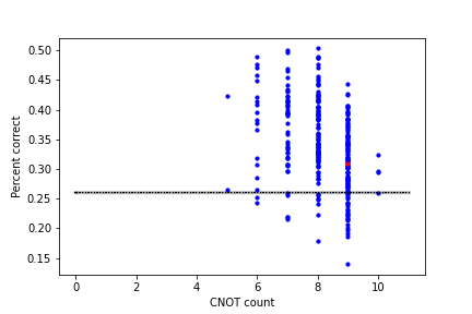
Figure 14. Probability of correct results over CNOT count of approximate circuits for 3 qubit Grover’s Algorithm on the Rome physical machine.

Figure 15 shows the result of the 4 qubit Toffoli and its approximates on a real machine. At first, the result looks similar to the distribution in Figure 6. However, while the best approximate circuits do have a much lower JS score (by 78%) than the reference circuit (orange), the reference circuit and many of the approximate circuits actually perform worse than random noise (as mentioned in the context of discussing Figure 7, random noise has a distance of 0.465).

This indicates that even the approximate circuits are still too noisy to run on the physical machines, but we expect them to perform better than the reference circuit when run on less noisy devices.

Observation 8: Trends indicate a continuing potential of approximate circuits to outperform reference circuits in the near future, even as noise levels in physical machines decline.

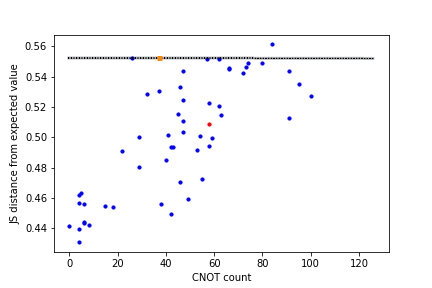
Figure 15. JS distance over CNOT count of approximate circuits for 4 qubit Toffoli on the Manhattan physical machine.

6.4. Sensitivity to Qubit Mappings on IBM Q Hardware

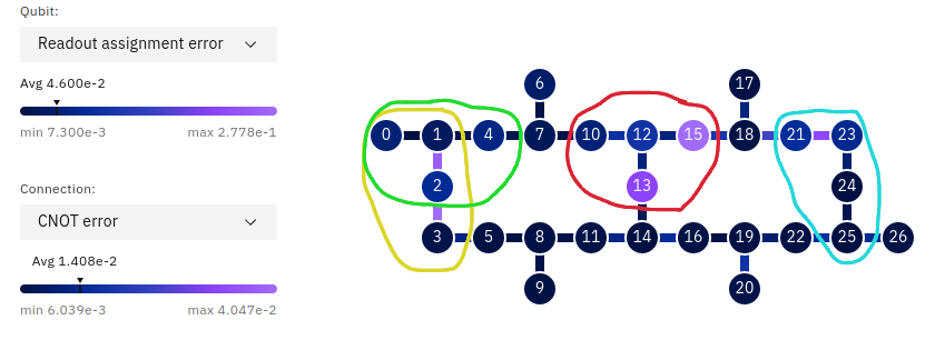
Figure 16. Noise report from IBM for their Toronto machine at the time of study. Different circles represent different mappings.

We further investigate the impact of mapping circuits to specific qubits with CNOT resonance channels of different noise levels for the IBM Toronto physical quantum device using the 4 qubit Toffoli. The qubit connectivity of this machine is shown in Figure 16, as reported by IBM on the day of experimentation. The nodes represent different qubits, and their color indicates the readout error in the range depicted on the upper heatmap index to the left. The edges represent the connection between the qubits, and their color indicates the CNOT error level on the lower heatmap index.

Experiments are conducted with four different (manual) mappings for the approximate circuits plus one (automatic) mapping using Qiskit’s transpiler at optimization level 3. We depict only the circuits with the best and worst results here.

Figure 17 shows results for circuits mapped onto the qubits within the blue circle in Figure 16. These results exhibit the shortest JS distance of $\approx$0.4 (best), and about a third of the circuits lie below the reference of $\approx$0.47.

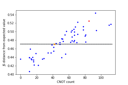
Figure 17. JS distance over CNOT count of approximate circuits for 4 qubit Toffoli on the Toronto physical machine showing the best performing mapping.

Figure 18 depicts the results for mappings into the red circle, which provided the worst results with higher JS distance (reference: JS$\approx$ 0.485, approximate circuits start at JS$\approx$0.45) than that of any other mapping. Other mappings (not depicted) lie in between these results.

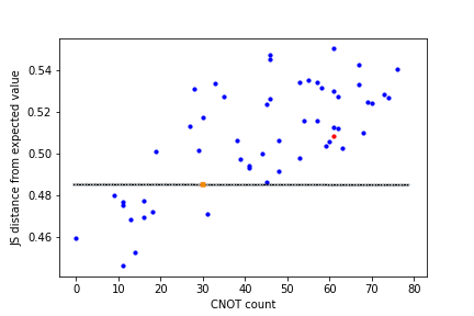
Figure 18. JS distance over CNOT count of approximate circuits for 4 qubit Toffoli on the Toronto physical machine showing the worst performing mapping.

Figure 19 shows the results of transpiling the same approximate circuits with Qiskit under level three optimizations. As each approximate circuit was mapped individually and automatically by Qiskit, no single mapping can be reported. The green circle shows the mapping for the best performing circuit within that run, and yellow indicates that of the reference circuit. Fewer circuits have a lower JS than the reference ($\approx.$ 0.46) but they start as JS$\approx$0.42.

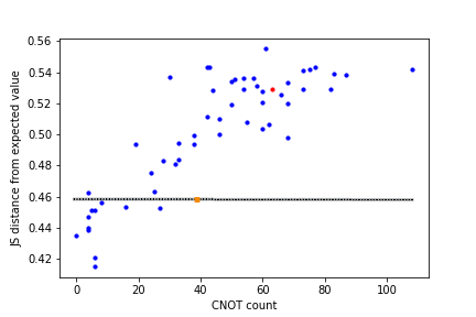
Figure 19. JS distance over CNOT count of approximate circuits for 4 qubit Toffoli on the Toronto physical machine showing mappings generated by Qiskit with optimization level 3.

These results are interesting when considering the noise levels in Figure 16. The yellow reference circuit (with results in Figure 19) chooses two connections with relatively high noise and utilizes about 40 CNOTs, but qubits have relatively high readout fidelity. Nonetheless, it performs better than than the reference circuit in Figure 18, which has relatively good connections and only 30 CNOTs. The results indicate that CNOT error cannot be the only source of noise influencing results.

Likewise, the blue mapping has one bad connection, but it provides the best performing circuits (Figure 17) with about the same readout fidelity as for yellow. The worst results (Figure 18) contribute few (if any) good circuits, yet benefit from relatively good connections but lower readout fidelity according to IBM’s noise data.

We know from Observation 6 that increasing CNOT error provides additional opportunities for approximate circuits. Our mapping study is an indication that other noise sources contribute as well, particularly read-out errors (as depicted in Figure 16) as well as cross-talk (not reported by IBM but also known to be of the same magnitude). This aspect requires further investigation.

Observation 9: Sources other than CNOT error appear to contribute to the performance of approximate circuits.

6.5. Roadmap and Future Work

Noisy gates enable and encourage circuit approximations. We plan to extend this study and correlate circuit behavior with commonly accepted hardware evaluation metrics, such as gate, read-out, and cross-talk fidelity, and also “quantum volume” (Bishop2017QuantumV, ). This will allow us to project the potential of approximations in the face of continuous hardware evolution and decreasing noise. Metrics such as quantum volume capture the impact of the relatively short chip coherence times. A “small” quantum volume indicates there are empirical practical bounds on the circuit depth, where we can expect approximations to benefit. Finally, best circuit selection is performed using simulation/execution and examining the result in its specific context. In order to guide circuit generation and synthesis from first principles, we are interested in a thorough analysis of the numerical value of different metrics (Hilbert-Schmidt distance (Gilchrist_2005, ), Kullback-Leibler divergence (Kullback_1951, ), Jensen-Shannon distance (endres_03, ), etc.)

We are also looking into both deeper and wider circuits. QSearch begins to require a prohibitive amount of search time when exposing it to more than four qubits. QFast is a little faster and can typically work with up to six qubits, but is still restricted in the number of qubits it can handle. The Berkeley Quantum Synthesis Kit recently acquired another method of synthesis, QFactor (qfactor, ), with the ability to synthesize circuits of up to eight qubits. QFactor may be able to create approximate circuits in that range, but a new method of developing approximate circuits is needed for even wider circuits.

One possible solution to consider is that of breaking a large program into pieces; it may be possible to create a large circuit out of many small circuits, and we are interested in assessing if approximate circuits also prove to be useful in such a context.

7. Related Work

While finding an approximate circuit is typically seen as less desirable than finding an exact circuit, much work has been put in in an effort to finding approximate circuits. The Solovay-Kitaev algorithm (SK2005, ) is well known to generate quantum gates which have a specified accuracy.

Work on circuit synthesis (qs, ; qfast, ; Amy2013, ; DeVos2015, ) is often classified as either “exact” or “approximate”. But even the approximate algorithms often end up finding closer approximations for circuits than those we are interested in; the small allowable error does not add enough wiggle room to take advantage of short circuits. We are most interested in $\epsilon$-approximate synthesis techniques, which can be coarsened to find circuits which are “more approximate”. Closely related is the Quantum Fast Circuit Optimizer (QFactor) (qfactor, ), a newly developed piece of synthesis software being distributed as part of the Berkeley Quantum Synthesis Toolkit, just as QSearch and QFast are. It can handle a greater number of qubits than QSearch and QFast can, but is focused more on circuit optimization than just synthesis, and works through tensor networks.

The Quantum Approximate Optimization Algorithm (QAOA) (farhi2015quantum, ) can also be said to create approximate circuits, though it differs from the work done here in that there is not a known target circuit. Much work has gone into optimizing QAOA circuits. Especially interesting with relation to this work is the work of (alam20, ), which reorders gates in order to reduce circuit length, similarly finding that approximate circuits with fewer CNOTs tend to outperform approximate circuits with more.

Much more work is being done on other ways to reduce noise or circuit depth (ding20, ; Murali2019, ; li2019tackling, ; wilson20, ; gokhale20, ; ibm-pulses, ; wille2016look, ). We are optimistic about these being able to work alongside approximate circuits, though it is unclear whether the benefits of approximate circuits will hold for process which require post-processing or manipulation of error levels, as these may end up interfering with the noise which the approximate circuits rely on to perform better than exact circuits.

8. Conclusion

Experimental results confirm that on NISQ devices approximate circuits have the potential to outperform theoretically precise reference circuits. Even though these circuits would perform worse on a perfect machine, if they are created to be similar to the reference circuits but have fewer CNOT gates, these approximate circuits produce higher fidelity results.

Because these improvements rely on reducing the number of CNOT gates, we see approximate circuits perform best relative to reference circuits in situations where the reference circuit has many CNOT gates, namely by up to 60% in experiments.

We have shown that approximate circuits can show greatly increased performance, but we have also shown that selecting the proper approximate circuit is more complicated than comparing process metrics. At the very least, target machine noise levels need to be taken into account. Finding a reliable way to determine the ideal approximate circuit remains an open problem.

References

- (1) J. Preskill, “Quantum computing in the NISQ era and beyond,” arXiv:1801.00862v3, vol. [quant-ph], 2018.
- (2) P. Murali, N. M. Linke, M. Martonosi, A. J. Abhari, N. H. Nguyen, and C. H. Alderete, “Full-stack, real-system quantum computer studies: Architectural comparisons and design insights,” in International Symposium on Computer Architecture, 2019, pp. 527–540.
- (3) P. Murali, J. M. Baker, A. J. Abhari, F. T. Chong, and M. Martonosi, “Noise-adaptive compiler mappings for noisy intermediate-scale quantum computers,” arXiv preprint arXiv:1901.11054, 2019.
- (4) E. Wilson, S. Singh, and F. Mueller, “Just-in-time quantum circuit transpilation reduces noise,” in IEEE International Conference on Quantum Computing and Engineering (QCE), Oct. 2020.
- (5) A. JavadiAbhari, S. Patil, D. Kudrow, J. Heckey, A. Lvov, F. T. Chong, and M. Martonosi, “ScaffCC: A framework for compilation and analysis of quantum computing programs,” in Proceedings of the 11th ACM Conference on Computing Frontiers, ser. CF ’14. New York, NY, USA: ACM, 2014, pp. 1:1–1:10. [Online]. Available: http://doi.acm.org/10.1145/2597917.2597939
- (6) L. Bishop and J. Gambetta, “Reduction and/or mitigation of crosstalk in quantum bit gates,” 2019, US Patent App. 15/721,194.
- (7) D. C. McKay, T. Alexander, L. Bello, M. J. Biercuk, L. Bishop, J. Chen, J. M. Chow, A. D. Córcoles, D. Egger, S. Filipp, J. Gomez, M. Hush, A. Javadi-Abhari, D. Moreda, P. Nation, B. Paulovicks, E. Winston, C. J. Wood, J. Wootton, and J. M. Gambetta, “Qiskit backend specifications for OpenQASM and OpenPulse experiments,” preprint arXiv:1809.03452, 2018.
- (8) A. Zulehner, A. Paler, and R. Wille, “An efficient methodology for mapping quantum circuits to the IBM QX architectures,” IEEE Transactions on Computer-Aided Design of Integrated Circuits and Systems, 2018.
- (9) S. S. Tannu and M. K. Qureshi, “Ensemble of diverse mappings: Improving reliability of quantum computers by orchestrating dissimilar mistakes,” in International Symposium on Microarchitecture, 2019, pp. 253–265.
- (10) ——, “Mitigating measurement errors in quantum computers by exploiting state-dependent bias,” in International Symposium on Microarchitecture, 2019, pp. 279–290.
- (11) ——, “Not all qubits are created equal: A case for variability-aware policies for NISQ-era quantum computers,” in Proceedings of the Twenty-Fourth International Conference on Architectural Support for Programming Languages and Operating Systems, 2019.
- (12) G. Li, Y. Ding, and Y. Xie, “Tackling the qubit mapping problem for NISQ-era quantum devices,” in Architectural Support for Programming Languages and Operating Systems, 2019, pp. 1001–1014.
- (13) ——, “Towards efficient superconducting quantum processor architecture design,” in Conference on Architectural Support for Programming Languages and Operating Systems, 2020.
- (14) R. Wille, O. Keszocze, M. Walter, P. Rohrs, A. Chattopadhyay, and R. Drechsler, “Look-ahead schemes for nearest neighbor optimization of 1D and 2D quantum circuits,” in 2016 21st Asia and South Pacific Design Automation Conference (ASP-DAC). IEEE, 2016, pp. 292–297.
- (15) M. Y. Siraichi, V. F. d. Santos, S. Collange, and F. M. Q. Pereira, “Qubit allocation,” in Proceedings of the 2018 International Symposium on Code Generation and Optimization. ACM, 2018, pp. 113–125.
- (16) P. Murali, D. C. Mckay, M. Martonosi, and A. Javadi-Abhari, “Software mitigation of crosstalk on noisy intermediate-scale quantum computers,” in Proceedings of the Twenty-Fifth International Conference on Architectural Support for Programming Languages and Operating Systems, ser. ASPLOS ’20. New York, NY, USA: Association for Computing Machinery, 2020, p. 1001–1016. [Online]. Available: https://doi.org/10.1145/3373376.3378477
- (17) Y. Ding, P. Gokhale, S. Lin, R. Rines, T. Propson, and F. T. Chong, “Systematic crosstalk mitigation for superconducting qubits via frequency-aware compilation,” in 2020 53rd Annual IEEE/ACM International Symposium on Microarchitecture (MICRO). Los Alamitos, CA, USA: IEEE Computer Society, oct 2020, pp. 201–214. [Online]. Available: https://doi.ieeecomputersociety.org/10.1109/MICRO50266.2020.00028
- (18) M. Amy, D. Maslov, M. Mosca, and M. Roetteler, “A meet-in-the-middle algorithm for fast synthesis of depth-optimal quantum circuits,” IEEE Transactions on Computer-Aided Design of Integrated Circuits and Systems, vol. 32, no. 6, pp. 818–830, 2013.
- (19) A. De Vos and S. De Baerdemacker, “The block-zxz synthesis of an arbitrary quantum circuit,” Physical Review A, 2015.
- (20) M. Alam, A. Ash-Saki, and S. Ghosh, “Circuit compilation methodologies for quantum approximate optimization algorithm,” in 2020 53rd Annual IEEE/ACM International Symposium on Microarchitecture (MICRO). Los Alamitos, CA, USA: IEEE Computer Society, oct 2020, pp. 215–228. [Online]. Available: https://doi.ieeecomputersociety.org/10.1109/MICRO50266.2020.00029
- (21) M. G. Davis, E. Smith, A. Tudor, K. Sen, I. Siddiqi, and C. Iancu, “Heuristics for quantum compiling with a continuous gate set,” 2019.
- (22) E. Younis, K. Sen, K. Yelick, and C. Iancu, “Qfast: Quantum synthesis using a hierarchical continuous circuit space,” 2020.
- (23) A. Gilchrist, N. K. Langford, and M. A. Nielsen, “Distance measures to compare real and ideal quantum processes,” Physical Review A, vol. 71, no. 6, Jun 2005. [Online]. Available: http://dx.doi.org/10.1103/PhysRevA.71.062310
- (24) D. Aharonov, A. Kitaev, and N. Nisan, “Quantum circuits with mixed states,” in Proceedings of the Thirtieth Annual ACM Symposium on Theory of Computation (STOC), 1997, pp. 20–30.
- (25) D. M. Endres and J. E. Schindelin, “A new metric for probability distributions,” IEEE Transactions on Information Theory, vol. 49, no. 7, pp. 1858–1860, 2003.
- (26) H. Abraham, AduOffei, I. Y. Akhalwaya, and et al., “Qiskit: An open-source framework for quantum computing,” 2019. [Online]. Available: qiskit.org
- (27) C. J. Wood, “Introducing Qiskit Aer: A high performance simulator framework for quantum circuits,” https://medium.com/qiskit/qiskit-aer-d09d0fac7759.
- (28) L. Bassman, K. Liu, A. Krishnamoorthy, T. Linker, Y. Geng, D. Shebib, S. Fukushima, F. Shimojo, R. K. Kalia, A. Nakano et al., “Towards simulation of the dynamics of materials on quantum computers,” Physical Review B, vol. 101, no. 18, p. 184305, 2020.
- (29) L. Bassman, R. V. Beeumen, E. Younis, E. Smith, C. Iancu, and W. A. de Jong, “Constant-depth circuits for dynamic simulations of materials on quantum computers,” 2021.
- (30) L. K. Grover, “A fast quantum mechanical algorithm for database search,” in Proceedings of the Twenty-Eighth Annual ACM Symposium on Theory of Computing. New York, New York, USA: ACM, 1996, pp. 212–219.
- (31) T. Toffoli, “Reversible computing,” in Automata, Languages and Programming, J. de Bakker and J. van Leeuwen, Eds. Berlin, Heidelberg: Springer Berlin Heidelberg, 1980, pp. 632–644.
- (32) L. Bishop, S. Bravyi, A. Cross, J. Gambetta, J. Smolin, and March, “Quantum volume,” 2017.
- (33) S. Kullback and R. A. Leibler, “On Information and Sufficiency,” The Annals of Mathematical Statistics, vol. 22, no. 1, pp. 79 – 86, 1951. [Online]. Available: https://doi.org/10.1214/aoms/1177729694
- (34) E. Younis, “Bqskit/qfactor.” [Online]. Available: https://github.com/bqskit/qfactor
- (35) C. M. Dawson and M. A. Nielsen, “The solovay-kitaev algorithm,” Quantum Information and Computation, 2005.
- (36) E. Farhi, J. Goldstone, and S. Gutmann, “A quantum approximate optimization algorithm applied to a bounded occurrence constraint problem,” 2015.
- (37) P. Gokhale, A. Javadi-Abhari, N. Earnest, Y. Shi, and F. T. Chong, “Optimized quantum compilation for near-term algorithms with openpulse,” in 2020 53rd Annual IEEE/ACM International Symposium on Microarchitecture (MICRO). Los Alamitos, CA, USA: IEEE Computer Society, oct 2020, pp. 186–200. [Online]. Available: https://doi.ieeecomputersociety.org/10.1109/MICRO50266.2020.00027