An exactly solvable problem of wave fronts
and applications to the asymptotic theory

Abstract.

This is the full and extended version of the brief note arxiv.org/abs/1908.00938. A nontrivially solvable 4-dimensional Hamiltonian system is applied to the problem of wave fronts and to the asymptotic theory of partial differential equations. The Hamilton function we consider is $H(\mathbf{x},\mathbf{p})=\sqrt{D(\mathbf{x})}|\mathbf{p}|$. Such Hamiltonians arise when describing the fronts of linear waves generated by a localized source in a basin with a variable depth. We consider two realistic types of bottom shape: 1) the depth of the basin is determined, in the polar coordinates, by the function $D(\varrho,\varphi)=(\varrho^{2}+b)/(\varrho^{2}+a)$ and 2) the depth function is $D(x,y)=(x^{2}+b)/(x^{2}+a)$. As an application, we construct the asymptotic solution to the wave equation with localized initial conditions and asymptotic solutions of the Helmholtz equation with a localized right-hand side.

Introduction

In the present paper we consider an exactly solvable Hamiltonian system

$$\dot{\mathbf{x}}=H_{\mathbf{p}}\mskip 1.0mu,\quad\dot{\mathbf{p}}=-H_{\mathbf{x}}\mskip 1.0mu,\quad\mathbf{x},\mathbf{p}\in\mathbb{R}^{2}$$ (1)

with the Hamiltonian

$$H=|\mathbf{p}|C(\mathbf{x}),\quad C(\mathbf{x})=\sqrt{gD(\mathbf{x})}$$ (2)

and an associated problem of the wave fronts under the initial conditions

$$\mathbf{p}|_{t=t_{\circ}}=\mathbf{n}(\psi)=\begin{pmatrix}\cos\psi\\ \sin\psi\end{pmatrix},\quad\psi\in[0,2\pi],\quad\mathbf{x}|_{t=t_{\circ}}=\mathbf{x}^{\circ}\in\mathbb{R}^{2}\mskip 1.0mu.$$ (3)

The function $D(\mathbf{x})$ is assumed to be one of two types, which will be given bellow. Solutions to these problems can then be represented in terms of elliptic functions [1].

Among other things the Hamiltonian systems of that sort arise in the study of waves generated by a localized source. This problem, in turn, appears in modeling the tsunami waves [20] and mesoscale eddies in the ocean. It is well known [22, 20] that the long-wave approximation in an infinite basin with a variable depth defined by the function $D(\mathbf{x})>0$ leads to the linear wave equation of the form

$$\frac{\partial^{2}w}{\partial t^{2}}-\big{\langle}\nabla,C^{2}(\mathbf{x})\nabla\big{\rangle}w=0,\quad C^{2}(\mathbf{x})=gD(\mathbf{x}),\quad\mathbf{x}\in\mathbb{R}^{2}\mskip 1.0mu.$$ (4)

Here, $g$ is the gravity acceleration, $\nabla$ denotes the two-dimensional gradient, $\langle\cdot,\cdot\rangle$ is the usual scalar product, so $\big{\langle}\nabla,C^{2}(\mathbf{x})\nabla\big{\rangle}w=C^{2}(\mathbf{x})\Delta w+2C(\mathbf{x})(C^{\prime}_{x_{1}}w^{\prime}_{x_{1}}+C^{\prime}_{x_{2}}w^{\prime}_{x_{2}})$. For this equation we consider the Cauchy problem with localized initial conditions

$$w|_{t=0}=v\vbox{\hbox{\large$\Big{(}$}}\frac{\mathbf{x}-\mathbf{x}^{\circ}}{l}\vbox{\hbox{\large$\Big{)}$}},\quad\frac{\partial w}{\partial t}\Big{|}_{t=0}=0,$$ (5)

where smooth function $V(y)$ (that decreasing fast as $|y|\to\infty$) characterizes the uplift of the ocean surface, the parameter $l$ characterizes the source size, and $\mathbf{x}^{\circ}$ is a point in whose neighborhood the initial perturbation is localized.

To the best of our knowledge, the complete analytic solutions to problems of this kind are either absent or are somewhat artificial/non-realistic. On the other hand, the realistic Hamiltonians and depth-functions may lead, when solvable, to nontrivial representation problems with (elliptic) theta-functions, especially considering the fact that the ultimate formulas may give rise to the rather nonstandard inversion problems [3]. It is this situation—transcendental equations in sect.1—that arises in the procedure of integrating the system (1)–(2). In the theory of integrable systems [15, 9, 6], such equations correspond to a non-linear evolution on Jacobians and to inversion of meromorphic [2, 3] and logarithmic integrals rather than the holomorphic ones. See also [8, sect.9.2] for explicit formulas and monograph [15] for extensive bibliography along these lines.

It is also known that solvability in terms of elliptic functions [1] constitutes presently a school in its own right and impart the great analytic effectiveness to the general integrability-theory [6, 9]; even the ‘modular part’ of the elliptic theory—Weierstrass’ parameters $g_{2},g_{3}$—meets (nonstandard) inversion problems and has nontrivial applications [21].

As for the wave applications, we consider waves propagating over underwater banks and ridges. Accordingly, the function $D$ that determines the shape of the basin bottom has one of two types. In the case of a bank, the basin depth is defined by the function

$$D(\varrho,\varphi)=\frac{\varrho^{2}+b}{\varrho^{2}+a}\mskip 1.0mu$$ (6)

where $\varrho$ is a polar radius and $a>b>0$ are constants. For a ridge, the basin depth is defined by the function

$$D(\mathbf{x})=\frac{x_{1}^{2}+b}{x_{1}^{2}+a},\quad\mathbf{x}=(x_{1},x_{2})$$ (7)

with the same restriction on the constants $a$ and $b$. The exact analytical solutions of the corresponding Hamiltonian systems are given in sect.1.1 and sect.1.2 respectively.

The problem of constructing such solutions is interesting both in its own right and in applications. In particular, the system (1)–(2) arises when constructing the asymptotic solutions to the various boundary-value problems for the wave equation with a variable velocity $C(\mathbf{x})$ by application of the well-known in physics the ray method [5, sect.I]. This technique is based on the eikonal equation—the Hamilton–Jacobi equation for a Hamiltonian—and on the transport equations through a transition to the ray coordinates. Let us briefly describe the idea of the method and explain how the asymptotic solution of equation (4) is related to the Hamiltonian(2).

If the source-localization parameter $l$ tends to zero we may seek an asymptotic solution of the problem (4)–(5) in the form

$$w=f\vbox{\hbox{\large$\Big{(}$}}\frac{t-s(\mathbf{x})}{l},\mathbf{x},t\vbox{\hbox{\large$\Big{)}$}}+O(l)\mskip 1.0mu,$$

where $f(y,\mathbf{x})$ and $s(\mathbf{x})$ are smooth functions, and $f(y,\mathbf{x})$ is decreasing fast as $|y|\rightarrow\infty$. Substituting this ansatz into (4) and equating the coefficient at $l^{-2}$ to zero, we get the Hamilton–Jacobi equation for the function $s(\mathbf{x})$:

$$C(\mathbf{x})\sqrt{\left(\frac{\partial s(\mathbf{x})}{\partial x_{1}}\right)^{2}+\left(\frac{\partial s(\mathbf{x})}{\partial x_{2}}\right)^{2}}=\pm 1.$$ (8)

Note that the left-hand side of this equation is obtained from function (2) by replacing $p_{i}$ with $\frac{\partial s}{\partial x_{i}}$ ($i=1,2$). Equation (8) can thus be solved along characteristics $\mathbf{x}(\tau),\mskip 1.0mu\mathbf{p}(\tau)$ that are determined from the system (1)–(2); namely, $\mathbf{p}(\tau)=\frac{\partial s}{\partial\mathbf{x}}(\mathbf{x}(\tau))$ and $\frac{ds(\mathbf{x}(\tau))}{d\tau}=\langle\mathbf{p}(\tau),\frac{d\mathbf{x}(\tau)}{d\tau}\rangle=\pm 1$.

Solutions of the system (1)–(3) determine both rays—projections of the characteristics onto plane $(x_{1},x_{2})$ (the angle $\psi$ specifies the direction of the ray)—and the wave fronts. The wave front at time $t$ is a curve $s(\mathbf{x})=t$. Parenthetically, the generalized phase $S(\mathbf{x},t)$ is also determined by rays and $S(\mathbf{x},t)=0$ at front points. The choice of the initial conditions $\mathbf{x}(t)|_{t=t_{\circ}}=\mathbf{x}^{\circ}$ for the system (we release characteristics from the point $\mathbf{x}^{\circ}$) is explained by the fact that the initial condition (5) for the wave equation (4) is localized in a neighborhood of $\mathbf{x}^{\circ}$. If rays do not cross and fronts are smooth curves, then equation (8) is solved by passing from coordinates $(\tau,\psi)$ to $(x_{1},x_{2})$. The equating the coefficients at $l^{-1}$ to zero yields a transport equation for the function $f$, whose solution can also be obtained by the ray method. However, in the vicinity of the singularity of the rays’ field—focal points of fronts—one should use other methods, in particular, the method of the Maslov canonical operator. See the monographs [17, secs.III.8–12] and [18, secs.I.6–8] for details.

Let us give more precise definitions of the concepts mentioned earlier. Let $\mathbf{X}(\psi,t)$ and $\mathbf{P}(\psi,t)$ be a solution of the problem (1)–(3). Then the ray is by definition an $\mathbb{R}^{2}_{\mathbf{x}}$-subset $\{(x_{1},x_{2})=(X_{1}(\psi_{0},t),X_{2}(\psi_{0},t)):\mskip 1.0mut>0\}$ under the fixed $\psi_{0}\in[0,2\pi)$. At each moment of time $t$ the ends of trajectories define smooth closed curves $\Gamma_{t}=\{\mathbf{x}=\mathbf{X}(\psi,t),\mskip 1.0mu\mathbf{p}=\mathbf{P}(\psi,t)\}$ in the four-dimensional phase space $\mathbb{R}_{\mathbf{xp}}^{4}$.

Definition.

Curves $\Gamma_{t}$ are called the wave fronts in the phase space. Curves $\gamma_{t}=\{\mathbf{x}=\mathbf{X}(\psi,t),\psi\in S^{1}\}$, which are projections of $\Gamma_{t}$ on $\mathbb{R}_{\mathbf{x}}^{2}$, are called the wave fronts in the configuration space. The points of the fronts $\gamma_{t}$ wherein $\partial_{\psi}\mathbf{X}=0$ will be termed the focal points.

According to [12, 13, 10], at each moment of time $t$ an asymptotic solution of the problem (4)–(5) as $l\rightarrow 0$ is determined by $\Gamma_{t}$ and has been localized in a neighborhood of $\gamma_{t}$. Note that in contrast to $\Gamma_{t}$ the curves $\gamma_{t}$ may be nonsmooth and have points of self-intersection. Moreover, the asymptotic formulas differ in the neighborhood of nonfocal and focal points of the front. Thus, from the point of view of applications, a problem of visualizing the fronts is relevant. The corresponding algorithm is described in sect.2.1. Formulas for the asymptotic solution of the problem (4)–(5) as $l\rightarrow 0$ are given in sect.2.2.

This methodology can be further applied to the constructing the asymptotic solutions of a PDEs with a localized right-hand side. To illustrate, we consider an inhomogeneous equation

$$\frac{\partial^{2}u}{\partial t^{2}}-\big{\langle}\nabla,C^{2}(\mathbf{x})\nabla\big{\rangle}u=F(\mathbf{x},t),\quad\mathbf{x}\in\mathbb{R}^{2}.$$ (9)

Such equation describes the situation when a source acts over time, while the Cauchy problem (5) for the homogeneous wave equation (4) describes the instantaneous action of the source. Suppose that the source is harmonic in time and localized in space, i.e., let $F=\frac{1}{\varepsilon^{3}}e^{\frac{i}{\varepsilon}\omega t}\cdot V(\frac{\mathbf{x}-\mathbf{x}^{\circ}}{\varepsilon})$, with $\omega>0$. If we represent solution of equation (9) in the form $u=e^{\frac{i}{\varepsilon}\omega t}v$ we obtain the Helmholtz equation

$$-\omega^{2}v-\varepsilon^{2}\big{\langle}\nabla,C^{2}(\mathbf{x})\nabla\big{\rangle}v=\frac{1}{\varepsilon}V\vbox{\hbox{\large$\Big{(}$}}\frac{\mathbf{x}-\mathbf{x}^{\circ}}{\varepsilon}\vbox{\hbox{\large$\Big{)}$}},\quad\mathbf{x}\in\mathbb{R}^{2}.$$ (10)

The work [4] describes an approach to the constructing the asymptotic solutions of inhomogeneous equations of this type. Using the Maupertuis–Jacobi method, we transform the original Hamiltonian $\mathscr{H}(\mathbf{x},\mathbf{p})=-\omega^{2}+C^{2}(\mathbf{x})|\mathbf{p}|^{2}$ for equation (10) (the differential operator $\mathscr{H}(\mathbf{x},\hat{\mathbf{p}}),\mskip 1.0mu\hat{\mathbf{p}}=-i\varepsilon\nabla$ defines the equation) to the Hamiltonian (2), which is considered in the present work. The exact formulas for the fronts allow us to obtain quiet simple expression for the asymptotic solution. An example pertaining to this situation is discussed in sect.2.3.

1. Analytical solutions

1.1. Underwater bank

Consider first a situation in which the bottom has the shape of underwater bank. This means that the basin depth is defined by the function (6). Since it is symmetric, without loss of generality we can assume that $\mathbf{x}^{\circ}=(-\xi,0)$, where $\xi>0$. We also put the free-fall acceleration to be equal to unity: $g=1$.

The polar symmetry guides us to pass to the polar coordinates

$$x_{1}=\varrho\cos\varphi,\quad x_{2}=\varrho\sin\varphi,$$

$$p_{1}=u\cos\varphi-\frac{1}{\varrho}v\sin\varphi,\quad p_{2}=u\sin\varphi+\frac{1}{\varrho}v\cos\varphi,$$ (11)

where $u:=p_{\varrho}$, $v:=p_{\varphi}$ are the momenta corresponding to the variables $(\varrho,\varphi)$. In these coordinates the Hamiltonian (2) acquires the form

$$\mathscr{H}(\varrho,\varphi;u,v)=\sqrt{u^{2}+\frac{v^{2}}{\varrho^{2}}}\cdot\sqrt{\frac{\varrho^{2}+b}{\varrho^{2}+a}}$$ (12)

and initial conditions (3) become

$$u|_{t=t_{\circ}}=-\cos\psi,\quad v|_{t=t_{\circ}}=-\xi\sin\psi,\quad\varrho|_{t=t_{\circ}}=\xi,\quad\varphi|_{t=t_{\circ}}=\pi.$$ (13)

Since all the solutions to our models involve the elliptic integrals and functions, we shall adopt in what follows a shortened Weierstrass notation for them [1]:

$$\wp(z)=\wp(z;\alpha,\beta),\quad\zeta(z)=\zeta(z;\alpha,\beta),\quad\sigma(z)=\sigma(z;\alpha,\beta).$$

Proposition 1.

The solution of the Hamiltonian system (1)–(2) and (12) under the initial conditions (13) is given by the following expressions

$$\left\{\begin{aligned} \varrho&=\sqrt{\wp(\boldsymbol{\mathfrak{p}})+\delta-a},\\ \varphi&=\pi\pm\bigg{\{}1+2\mskip 1.0mub\mskip 1.0mu\frac{\zeta(\varkappa)}{\wp^{\prime}(\varkappa)}\bigg{\}}h\cdot(\boldsymbol{\mathfrak{p}}-\mathfrak{p}_{\circ})\pm\frac{b\mskip 1.0muh}{\wp^{\prime}(\varkappa)}\ln\frac{\sigma(\boldsymbol{\mathfrak{p}}-\varkappa)\mskip 1.0mu\sigma(\mathfrak{p}_{\circ}+\varkappa)}{\sigma(\boldsymbol{\mathfrak{p}}+\varkappa)\mskip 1.0mu\sigma(\mathfrak{p}_{\circ}-\varkappa)}\\ u&=-\frac{1}{2}\sqrt{\frac{\xi^{2}+b}{\xi^{2}+a}}\mskip 1.0mu\frac{\wp^{\prime}(\boldsymbol{\mathfrak{p}})}{\wp(\boldsymbol{\mathfrak{p}})+\delta-a+b}\mskip 1.0mu\frac{1}{\sqrt{\wp(\boldsymbol{\mathfrak{p}})+\delta-a}},\quad v=-\xi\sin\psi\end{aligned}\right.,$$ (14)

The functions $\boldsymbol{\mathfrak{p}}$, $\mathfrak{p}_{\circ}$, and $\varkappa$ are solutions of the transcendental equations

$$\wp(\mathfrak{p}_{\circ})=\xi^{2}-\delta+a\mskip 1.0mu,\quad\wp(\varkappa)=\frac{1}{3}(a+b-\mathfrak{h})\mskip 1.0mu,\quad t-t_{\circ}=\delta\cdot(\boldsymbol{\mathfrak{p}}-\mathfrak{p}_{\circ})-\zeta(\boldsymbol{\mathfrak{p}})+\zeta(\mathfrak{p}_{\circ})\mskip 1.0mu.$$ (15)

The expressions for $\delta$, $\alpha$ and $\beta$ in terms of parameters of the problem are as follows

$$\left\{\begin{aligned} \delta&=\frac{1}{3}\mskip 1.0mu({\mathfrak{h}}+2\mskip 1.0mua-b),\quad\alpha=\frac{4}{3}\mskip 1.0mu\big{(}{\mathfrak{h}}^{2}-2\mskip 1.0mu(a-2\mskip 1.0mub)\mskip 1.0mu{\mathfrak{h}}+a^{2}-a\mskip 1.0mub+b^{2}\big{)}\\[4.30554pt] \beta&=\frac{4}{27}\mskip 1.0mu\big{(}{\mathfrak{h}}-a+2\mskip 1.0mub\big{)}\big{(}2\mskip 1.0mu{\mathfrak{h}}^{2}-4\mskip 1.0mu(a-2\mskip 1.0mub){\mathfrak{h}}+(2\mskip 1.0mua-b)(a+b)\big{)}\end{aligned}\right.,$$ (16)

where

$$h^{2}=\mathrel{\mathop{:}}{\mathfrak{h}}=\xi^{2}\mskip 1.0mu\frac{\xi^{2}+a}{\xi^{2}+b}\sin^{2}\psi\mskip 1.0mu.$$ (17)

Remark 1.

All the quantities $\mathfrak{p}_{\circ}$, $\boldsymbol{\mathfrak{p}}$, and $\varkappa$ may be complex. They lie on the edges of the parallelogram $(0,\omega,\omega+\omega^{\prime},\omega^{\prime}),$ where $\omega$ is the pure real period of the Weierstrass function and $\omega^{\prime}$ is pure imaginary. Besides, $\boldsymbol{\mathfrak{p}}$ lies on the same edge of the parallelogram as $\mathfrak{p}_{\circ}$. It should be noted that equations (15) have infinitely many roots. Because of this, we assume that the roots from the first positive branch are taken. An algorithm which illustrates the formulas and this remark is discussed in sect.2.1.

Proof.

Since transformation (11) is canonical, the polar representation of the system under consideration has the same gradient form as (1). Solution of (1)–(3) thus boils down to integrating the equations

$$\dot{u} =-\mathscr{H}_{\varrho}\mskip 1.0mu, \dot{\varrho}=\frac{u\mskip 1.0mu\varrho}{\sqrt{u^{2}\varrho^{2}+v^{2}}}\mskip 1.0mu\sqrt{\frac{\varrho^{2}+b}{\varrho^{2}+a}}\qquad(=\mathscr{H}_{u}),$$

$$\dot{v} =0\mskip 1.0mu, \dot{\varphi}=\frac{(v/\varrho)}{\sqrt{u^{2}\varrho^{2}+v^{2}}}\mskip 1.0mu\sqrt{\frac{\varrho^{2}+b}{\varrho^{2}+a}}\qquad(=\mathscr{H}_{v})$$ (18)

with the Hamiltonian function (12) and initial conditions (13). We however do not use the canonicity of this transformation, because the mere form (18) suggests the scheme of obtaining the separable dynamical equations. For the same reason, nor do we resort to the standard separability theory (see, e.g. [7]),

Indeed, the following laws of conservation are obvious:

$$|p|c(\varrho)=c_{\circ},\quad c_{\circ}=c(|\xi|)\equiv\sqrt{\frac{b+\xi^{2}}{a+\xi^{2}}},\quad v=-\xi\sin\psi\mskip 1.0mu,$$ (19)

and we represent them through the free complex constants $\gamma$ and $h$:

$$v=\gamma\quad(=\mathrm{const})\mskip 1.0mu,\qquad\mathscr{H}^{2}(\varrho,\varphi;u,\gamma)=\vbox{\hbox{\large$\Big{(}$}}u^{2}+\frac{\gamma^{2}}{\varrho^{2}}\vbox{\hbox{\large$\Big{)}$}}\frac{\varrho^{2}+b}{\varrho^{2}+a}=\frac{\gamma^{2}}{h^{2}}\quad(=\mathrm{const})\mskip 1.0mu.$$ (20)

These constants are related with the initial conditions, and it is not difficult to see that these relationships are equivalent to the following ones:

$$\gamma=-\xi\sin\psi,\quad h^{2}=\xi^{2}\frac{a+\xi^{2}}{b+\xi^{2}}\sin^{2}\psi.$$

Let us ascertain the dynamics $\varrho=R(t)$. By rewriting the integral (20) in the form $\mathscr{H}(\varrho,\varphi;u,v)=\gamma/h$, we obtain identity $\sqrt{\frac{\varrho^{2}+b^{2}}{\varrho^{2}+a^{2}}}=\frac{\gamma}{h\sqrt{u^{2}+\gamma^{2}/\varrho}}$, whence one gets

$$\dot{\varrho}=\frac{(\gamma/h)\cdot u}{u^{2}+\gamma^{2}/\varrho^{2}}.$$ (21)

Expressing $u$ via variable $\varrho$ and using the integral $\mathscr{H}(\varrho,\varphi;u,v)=\gamma/h$, we obtain the autonomous dynamics for the function $\varrho$:

$$\varrho\mskip 1.0mu\dot{\varrho}=\frac{\sqrt{(\varrho^{2}+b)\vbox{\hbox{\small$\big{[}$}}\varrho^{2}(\varrho^{2}+a)-(\varrho^{2}+b)h^{2}\vbox{\hbox{\small$\big{]}$}}}}{(\varrho^{2}+a)}\mskip 1.0mu.$$

The change $\varrho^{2}+a=\mathrel{\mathop{:}}z$ suggests itself, and we derive

$$\frac{1}{2}\mskip 1.0mu\dot{z}=\frac{1}{z}\mskip 1.0mu\sqrt{(z-a+b)\vbox{\hbox{\small$\big{[}$}}z\mskip 1.0mu(z-a)-(z-a+b)h^{2}\vbox{\hbox{\small$\big{]}$}}}\mskip 1.0mu.$$

This dynamics is readily transformed into the integral form

$$\int\limits^{z}_{\infty}{z}\mskip 1.0mu\frac{dz}{w}=t\mskip 1.0mu,\qquad\begin{aligned} w^{2}\mathrel{\mathop{:}}={}&4\mskip 1.0mu\vbox{\hbox{\small$\big{[}$}}z\mskip 1.0mu(z-a)-(z-a+b)h^{2}\vbox{\hbox{\small$\big{]}$}}(z-a+b)=\\ ={}&4\mskip 1.0mu(z-A)(z-B)(z-C)\end{aligned}\mskip 1.0mu,$$ (22)

where constants $(A,B,C)$ can be expressed through the parameters of the problem $(a,b,\xi)$ and constants $(\gamma,h)$. As was mentioned in Introduction, we arrive at the problem of inversion of a meromorphic elliptic integral.

Let us reduce (22) to the canonical Weierstrass form. For this we make a shift

$$z\mathrel{{\mathchar 1081\relax}{\mathchar 1081\relax}\mathchar 1099\relax}s =z-\delta\mskip 1.0mu,\quad\delta\mathrel{\mathop{:}}=\frac{1}{3}\mskip 1.0mu(A+B+C)$$

in order to obtain the standard: $4\mskip 1.0mus^{3}-\alpha\mskip 1.0mus-\beta=4\mskip 1.0mu(z-A)\mskip 1.0mu(z-B)\mskip 1.0mu(z-C)$. Hence it follows that the new constants $(\alpha,\beta)$ are given by the expressions (16). Then equation (22) takes the form

$$\int\limits^{\varrho^{2}+a-\delta}_{\infty}\mskip-8.0mu\frac{(s+\delta)\mskip 1.0muds}{\sqrt{4\mskip 1.0mus^{3}-\alpha\mskip 1.0mus-\beta}}=t\qquad\mathrel{{\mathchar 1081\relax}{\mathchar 1081\relax}\mathchar 1099\relax}\qquad\varrho=R(t)\mskip 1.0mu$$

and its solution can be represented in terms of $\wp$-function as

$$\varrho=R(t)=\sqrt{\wp\big{(}{\mathfrak{p}}(t);\alpha,\beta\big{)}+\delta-a}.$$ (23)

Here, the function ${\mathfrak{p}}(t)$ is determined—in the full elliptic notation—from equation

$$\delta\cdot\boldsymbol{\mathfrak{p}}-\zeta(\boldsymbol{\mathfrak{p}};\alpha,\beta)=t,$$ (24)

and $\zeta(\boldsymbol{\mathfrak{p}};\alpha,\beta)$ is the associated Weierstrass zeta-function. It is related to the $\wp$-function by definition $\zeta^{\prime}(\boldsymbol{\mathfrak{p}};\alpha,\beta)=-\wp(\boldsymbol{\mathfrak{p}};\alpha,\beta)$. Let us adopt the solution $\varrho=R(t)$, i.e., formulas (23)–(24) for the case of an arbitrary initial condition $R(t_{\circ})=\varrho_{\circ}$. It is more convenient to represent it in a $\boldsymbol{\mathfrak{p}}$-parametric form:

$$\begin{aligned} \varrho=\sqrt{\wp(\boldsymbol{\mathfrak{p}})+\delta-a}\mskip 1.0mu,\quad t-t_{\circ}=\delta\cdot(\boldsymbol{\mathfrak{p}}-\mathfrak{p}_{\circ})-\zeta(\boldsymbol{\mathfrak{p}})+\zeta(\mathfrak{p}_{\circ}),\end{aligned}$$

$$\mathfrak{p}_{\circ}\mskip 1.0mu:\quad\sqrt{\wp(\mathfrak{p}_{\circ})+\delta-a}=\varrho_{\circ}\qquad\text{(initial condition)}\mskip 1.0mu.$$

The solution $u=U(t)$ can be derived from (20)–(21) and from the relation

$$\dot{\boldsymbol{\mathfrak{p}}}(t)=\frac{1}{\wp(\boldsymbol{\mathfrak{p}}(t))+\delta}.$$

Substituting the expression for $\varrho=R(t)$ we get the 3-rd formula in (14).

Consider now the solution $\varphi=\Phi(t)$. With use of the last equation of system (18) and expression (23), we obtain

$$\dot{\varphi}=\frac{h}{\varrho^{2}}\mskip 1.0mu\frac{\varrho^{2}+b}{\varrho^{2}+a}=h\vbox{\hbox{\large$\Big{(}$}}1+\frac{b}{\wp(\boldsymbol{\mathfrak{p}})+\delta-a}\vbox{\hbox{\large$\Big{)}$}}\frac{1}{\wp(\boldsymbol{\mathfrak{p}})+\delta}\mskip 1.0mu.$$

Note that we have used the integral (20) as a radical. Therefore the sign should be taken into consideration, and we understand $\pm h$ by the notation $h$. Thus,

$$\varphi=\varphi_{\circ}+h\mskip 1.0mu(\boldsymbol{\mathfrak{p}}-\mathfrak{p}_{\circ})+b\mskip 1.0muh\cdot\int\limits^{t}_{t_{\circ}}\frac{1}{\wp\vbox{\hbox{\small$\big{(}$}}\mathfrak{p}(t)\vbox{\hbox{\small$\big{)}$}}+\delta-a}\cdot\frac{dt}{\wp\vbox{\hbox{\small$\big{(}$}}\mathfrak{p}(t)\vbox{\hbox{\small$\big{)}$}}+\delta}.$$

Making the change of variable by equality $dt=(\wp(\boldsymbol{\mathfrak{p}})+\delta)\mskip 1.0mud\boldsymbol{\mathfrak{p}}$, one obtains

$$\varphi=\varphi_{\circ}+h\mskip 1.0mu(\boldsymbol{\mathfrak{p}}-\mathfrak{p}_{\circ})+b\mskip 1.0muh\cdot\int\limits^{\mathfrak{p}(t)}_{\mathfrak{p}_{\circ}}\frac{d\boldsymbol{\mathfrak{p}}}{\wp(\boldsymbol{\mathfrak{p}})-\lambda},\qquad\lambda\mathrel{\mathop{:}}=a-\delta\mskip 1.0mu.$$

This is nothing but the logarithmic elliptic integral, which can be easily evaluated [1]. We then arrive at formula

$$\varphi=\varphi_{\circ}+h\mskip 1.0mu(\boldsymbol{\mathfrak{p}}-\mathfrak{p}_{\circ})+\left.\frac{b\mskip 1.0muh}{\wp^{\prime}(\varkappa)}\bigg{\{}\ln\frac{\sigma^{2}(\boldsymbol{\mathfrak{p}}-\varkappa)}{\sigma^{2}(\boldsymbol{\mathfrak{p}})}-\ln\big{(}\wp(\boldsymbol{\mathfrak{p}})-\lambda\big{)}+2\mskip 1.0mu\zeta(\varkappa)\mskip 1.0mu\boldsymbol{\mathfrak{p}}\bigg{\}}\right|_{\mathfrak{p}_{\circ}}^{\boldsymbol{\mathfrak{p}}}\mskip 1.0mu,$$

where $\varkappa$ is defined by the equality $\lambda=\wp(\varkappa)$. This expression can be rewritten in terms of Weierstrass $\sigma$-functions alone:

$$\varphi={} \varphi_{\circ}\pm\bigg{\{}1+2\mskip 1.0mub\mskip 1.0mu\frac{\zeta(\varkappa)}{\wp^{\prime}(\varkappa)}\bigg{\}}h\cdot(\boldsymbol{\mathfrak{p}}-\mathfrak{p}_{\circ})\pm\frac{b\mskip 1.0muh}{\wp^{\prime}(\varkappa)}\ln\frac{\sigma(\boldsymbol{\mathfrak{p}}-\varkappa)\mskip 1.0mu\sigma(\mathfrak{p}_{\circ}+\varkappa)}{\sigma(\boldsymbol{\mathfrak{p}}+\varkappa)\mskip 1.0mu\sigma(\mathfrak{p}_{\circ}-\varkappa)}\mskip 1.0mu,$$

$$\varkappa\mathrel{\mathop{:}}={} \wp^{-1}\big{(}\tfrac{1}{3}(a+b-\mathfrak{h})\big{)}\mskip 1.0mu.$$

Invoking the initial condition (13), we get finally the solution (14). ∎

1.2. Underwater ridge

Consider now the underwater ridge. This means that the basin depth is defined be the function (7). As earlier we set the free-fall acceleration to unity. Then the Hamiltonian (2) has the form

$$\mathscr{H}(x_{1},x_{2};p_{1},p_{2})=\sqrt{p_{1}^{2}+p_{2}^{2}}\cdot\sqrt{\frac{x_{1}^{2}+b}{x_{2}^{2}+a}}\mskip 1.0mu,$$ (25)

$$(p_{1},p_{2})\mathrel{\mathop{:}}=(p_{x_{1}},p_{x_{2}}).$$

As in the previous section, by symmetry and without loss of generality, we may set $\mathbf{x}^{\circ}=(-\xi,0),$ $\xi>0$. The initial conditions (3) are thus as follows

$$x_{1}|_{t=t_{\circ}}=-\xi,\qquad x_{2}|_{t=t_{\circ}}=0,\qquad p_{1}|_{t=t_{\circ}}=\cos\psi,\qquad p_{2}|_{t=t_{\circ}}=\sin\psi.$$ (26)

Proposition 2.

The solution of the Hamiltonian system (1)–(2) and (25) under the initial conditions (26) is given by the following expressions

$$\left\{\begin{aligned} x_{1}&=-\sqrt{\wp(\boldsymbol{\mathfrak{p}};\alpha,\beta)+\delta-a},\quad x_{2}=\sqrt{1-\mathfrak{h}^{-1}}\cdot t+\sqrt{\mathfrak{h}-1}\mskip 1.0mu(b-a)\cdot(\boldsymbol{\mathfrak{p}}-\mathfrak{p}_{\circ})\\ p_{1}&=\frac{1}{2}\mskip 1.0mu\frac{\gamma}{\sqrt{\mathfrak{h}-1}}\frac{\wp^{\prime}\big{(}{\mathfrak{p}}(t)\big{)}}{\wp\big{(}{\mathfrak{p}}(t)\big{)}+\delta-a+b}\sqrt[-2]{\wp\big{(}{\mathfrak{p}}(t)\big{)}+\delta-a},\quad p_{2}=\gamma\end{aligned}\right.\mskip 1.0mu.$$ (27)

The functions $\boldsymbol{\mathfrak{p}}$ and $\mathfrak{p}_{\circ}$ are solutions of transcendental equations

$$\frac{1}{h}\mskip 1.0mu(t-t_{\circ})=\delta\cdot(\boldsymbol{\mathfrak{p}}-\mathfrak{p}_{\circ})-\zeta(\boldsymbol{\mathfrak{p}};\alpha,\beta)+\zeta(\mathfrak{p}_{\circ};\alpha,\beta)\mskip 1.0mu,\quad\mathfrak{p}_{\circ}=\wp^{-1}(\xi^{2}-\delta+a;\alpha,\beta)\mskip 1.0mu.$$ (28)

The expressions for $\delta$, $\alpha$ and $\beta$ in terms of parameters of the problem are as follows

$$\left\{\begin{aligned} \delta&=\frac{1}{3}\mskip 1.0mu\big{(}(b-a)\mskip 1.0mu\mathfrak{h}+3\mskip 1.0mua-2\mskip 1.0mub\big{)},\quad\alpha=\frac{4}{3}\mskip 1.0mu\big{(}(b-a)^{2}\mathfrak{h}^{2}-(b-a)\mskip 1.0mub\mskip 1.0mu\mathfrak{h}+b^{2}\big{)}\\[4.30554pt] \beta&=\frac{4}{27}\mskip 1.0mu\big{(}(b-a)\mskip 1.0mu\mathfrak{h}+b\big{)}\big{(}(b-a)\mskip 1.0mu\mathfrak{h}-2\mskip 1.0mub\big{)}\big{(}2\mskip 1.0mu(b-a)\mskip 1.0mu\mathfrak{h}-b\big{)}\end{aligned}\right.\mskip 1.0mu,$$ (29)

where

$$\mathfrak{h}=\frac{\xi^{2}+b}{(\xi^{2}+b)-\sin^{2}\psi(\xi^{2}+a)},\quad\gamma=\sin\psi.$$

Proof.

The Hamiltonian system with the Hamiltonian (25) has the form

$$\dot{p}_{1} =-\mathscr{H}_{x_{1}}\mskip 1.0mu, \dot{x}_{1}=\frac{p_{1}}{\sqrt{p_{1}^{2}+p_{2}^{2}}}\mskip 1.0mu\sqrt{\frac{x_{1}^{2}+b}{x_{1}^{2}+a}}\qquad(=\mathscr{H}_{p_{1}}),$$

$$\dot{p}_{2} =0\mskip 1.0mu, \dot{x}_{2}=\frac{p_{2}}{\sqrt{p_{1}^{2}+{p_{2}}^{2}}}\mskip 1.0mu\sqrt{\frac{x_{1}^{2}+b}{x_{1}^{2}+a}}\qquad(=\mathscr{H}_{p_{2}}).$$ (30)

Using laws of conservation, we obtain

$$p_{2}=\gamma\qquad(=\mathrm{const})\mskip 1.0mu,\qquad(p_{1}^{2}+\gamma^{2})\mskip 1.0mu\frac{x_{1}^{2}+b}{x_{1}^{2}+a}=\frac{\gamma^{2}\mskip 1.0muh^{2}}{h^{2}-1}\qquad(=\mathrm{const})\mskip 1.0mu.$$ (31)

Here, $\gamma$ and $h$ are the complex constants related to initial conditions of the problem through the formulas

$$\gamma=\sin\psi,\qquad\frac{\xi^{2}+b}{\xi^{2}+a}=\frac{\gamma^{2}\mskip 1.0mu\mathfrak{h}}{\mathfrak{h}-1}\qquad(\mathfrak{h}\mathrel{\mathop{:}}=h^{2})\mskip 1.0mu,$$ (32)

and $(a,b,\xi)$ are parameters of the problem.

Let us ascertain the dynamics $x_{1}=X_{1}(t)$. Using the integral $\mathscr{H}(x_{1},x_{2};p_{1},p_{2})=\frac{\gamma h}{\sqrt{\mathfrak{h}-1}}$, we obtain

$$\dot{x}_{1}=\frac{p_{1}}{p_{1}^{2}+\gamma^{2}}\cdot\frac{\gamma\mskip 1.0muh}{\sqrt{\mathfrak{h}-1}}\mskip 1.0mu.$$ (33)

Acting in the same way as in the previous case, we derive the dynamics for the variable $x_{1}$

$$x_{1}\mskip 1.0mu\dot{x}_{1}=\frac{\sqrt{x_{1}^{2}\big{(}x_{1}^{2}+b\big{)}\big{(}x_{1}^{2}-(\mathfrak{h}-1)(b-a)\big{)}}}{h(x_{1}^{2}+a)}.$$

The change $z\mathrel{\mathop{:}}=x_{1}^{2}+a$ gives rise again to a meromorphic integral:

$$\int\limits_{t_{\circ}}^{z}z\mskip 1.0mu\frac{dz}{w}=\frac{1}{h}\cdot(t-t_{\circ})\mskip 1.0mu,\qquad\begin{aligned} w^{2}\mathrel{\mathop{:}}={}&4\mskip 1.0mu(z-a)(z-a+b)\big{(}z-(\mathfrak{h}-1)\mskip 1.0mu(b-a)\big{)}=\\ ={}&4\mskip 1.0mu(z-a)(z-a+b)(z-C).\end{aligned}$$

As previously, we reduce this expression to the canonical form by a shift $z\mathrel{{\mathchar 1081\relax}{\mathchar 1081\relax}\mathchar 1099\relax}s=z-\delta$ in order to obtain the Weierstrassian standard: $4\mskip 1.0mus^{3}-\alpha\mskip 1.0mus-\beta=4\mskip 1.0mu(z-a)\mskip 1.0mu(z-a+b)\mskip 1.0mu(z-C)$. Hence, the constant $\delta$ and invariants of elliptic functions $\alpha$ and $\beta$ are calculated through $a,b,\xi,\psi$; these are expressions (29).

The solution has the same structure as in the previous case:

$$\begin{aligned} x_{1}=\pm\sqrt{\wp\big{(}\mathfrak{p}(t);\alpha,\beta\big{)}-(a-\delta)},\\[4.30554pt] \delta\cdot(\boldsymbol{\mathfrak{p}}-\mathfrak{p}_{\circ})-\zeta(\boldsymbol{\mathfrak{p}};\alpha,\beta)+\zeta(\mathfrak{p}_{\circ};\alpha,\beta)&=\frac{1}{h}\cdot(t-t_{\circ}),\end{aligned}$$

$$\mathfrak{p}_{\circ}\mskip 1.0mu:\quad\sqrt{\wp(\mathfrak{p}_{\circ})+\delta-a}=\xi\qquad\text{(initial condition)}\mskip 1.0mu.$$

Using (31), (33) and the relation

$$\dot{\mathfrak{p}}(t)=\frac{1}{h}\mskip 1.0mu\frac{1}{\wp\vbox{\hbox{\small$\big{(}$}}{\mathfrak{p}}(t)\vbox{\hbox{\small$\big{)}$}}+\delta}\mskip 1.0mu,$$

we do substitute $x_{1}=X_{1}(t)$ found above and obtain solution $p_{1}=P_{1}(t)$ displayed in (27).

Let us determine the dynamics $x_{2}=X_{2}(t)$. From the last equation of the system (30) one obtains

$$\dot{x}_{2}=\sqrt{1-\mathfrak{h}^{-1}}\mskip 1.0mu\frac{x_{1}^{2}+b}{x_{1}^{2}+a}=\sqrt{1-\mathfrak{h}^{-1}}\vbox{\hbox{\large$\Big{(}$}}1+\frac{b-a}{\wp(\boldsymbol{\mathfrak{p}})+\delta}\vbox{\hbox{\large$\Big{)}$}}\mskip 1.0mu.$$

Hence,

$$x_{2}=x_{2}^{\circ}+\sqrt{1-\mathfrak{h}^{-1}}\cdot(t-t_{\circ})+\sqrt{1-\mathfrak{h}^{-1}}\mskip 1.0mu(b-a)\cdot\int\limits^{t}_{t_{\circ}}\frac{dt}{\wp\vbox{\hbox{\small$\big{(}$}}{\mathfrak{p}}(t)\vbox{\hbox{\small$\big{)}$}}+\delta}\mskip 1.0mu.$$

Rewriting the last integral in terms of elliptic functions, we arrive at (27). No use is required of the $\sigma$-functions in this case. ∎

2. Applications to asymptotic theory

In this section we discuss some applications of obtained analytical solutions to the asymptotic theory. We rely on the results by Dobrokhotov, Nazaikinskii, Shafarevich, and by others [4, 10, 11, 12, 13] in their study of the linear shallow-water waves, which are generated by a localized source and propagate in the basin with a variable depth. The method used is based on a modification of the Maslov canonical operator [18, secs.I.6–8]. One of the advantages of this method is that it gives the convenient asymptotic formulas in the neighborhood of focal points and caustics. Thus, the analytical formulas for solutions of the Hamiltonian systems under consideration allow us, among other things, to seek focal points. We also note that the turning points at the wave fronts are focal. Thereby visualization of the fronts can be considered as one of the applications.

2.1. Visualization of fronts. The algorithm

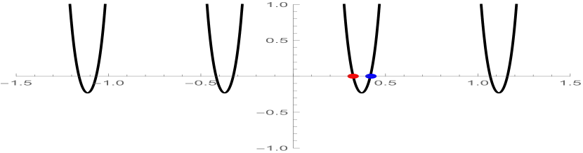
Figure 1. Graph $y=\wp(x)-\xi^{2}+\delta-a$ under $\psi=\frac{9\pi}{10}$

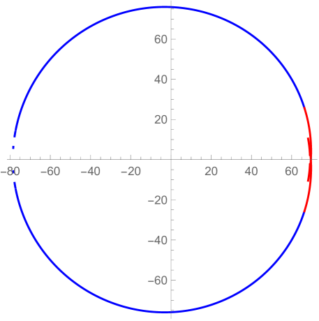
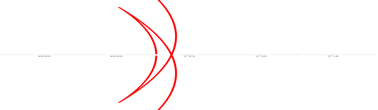
Figure 2. Graph of front under $t=100$

Here we describe an algorithm for constructing the fronts $\gamma_{t}$; it has been implemented with use of the software package Wolfram Mathematica and intensively exploits the elliptic transcendents. Except for visualizating the fronts and focal points, the algorithm can be applied to the asymptotic theory and allows us to determine the structure of Lagrangian manifolds [19, sect.2.1] and to construct the asymptotic solutions of other problems. In particular, the problem (4)–(5) is solved with use of the ray method or the Maslov canonical operator theory, which is its generalization. We will briefly describe the idea of Maslov’s theory further bellow. Moreover, as mentioned earlier, the asymptotic solution of the problem (4)–(5) is localized in the neighborhood of the front [12, 13, 10].

Algorithm:

1. Fix first the parameters of the problem and, by way of illustration, consider the case of underwater bank (sect.1.1). Constants $a$, $b$ determine the bottom shape and constant $\xi$ define the source position. We take the following values: $a=100$, $b=1$, and $\xi=0.5.$

2. For each fixed $\psi\in[0,\pi]$, there exist infinitely many roots of the equation

$$\wp(p_{0})=\xi^{2}-\delta+a.$$ (34)

As values of $p_{01}(\psi)$ and $p_{02}(\psi)$ we choose the first and second positive roots respectively (see Fig.2). In this figure, the red point corresponds to $p_{01}$ and the blue point corresponds to $p_{02}$. The quantity $\varkappa(\psi)$ is determined by the formula (15), where we take again the first positive root.

Remark 2.

As mentioned above, the roots of the equation (34) need not to be real. We have to seek the complex roots in one of the forms ${\mathrm{i}}\mskip 1.0mup_{0}$, $p_{0}+\omega^{\prime}$, or ${\mathrm{i}}\mskip 1.0mup_{0}+\omega$, where $\omega$ is the pure real period of the Weierstrassian $\wp$, and $\omega^{\prime}$ is its pure imaginary period; the $p_{0}$ is real. Hence we obtain some equation for $p_{0}$, which has infinitely many solutions. As $p_{01}$ and $p_{02}$ we must take, respectively, the nearest first and second positive roots (roots from the first positive branch).

3. Fix further the point of time $t$. Let $p_{i}(\psi,t)$ $(i=1,2)$ be the first positive root of the equation

$$t=\delta\cdot(p-p_{0i}(\psi))-\zeta(p)+\zeta(p_{0i}(\psi))\quad(i=1,2).$$

If $p_{0i}$ is not real, then we should seek $p_{i}$ in the same manner as $p_{0i}$; i.e., on the same edge of the parallelogram.

4. For each fixed $t$ we plot the curves in polar coordinates $\varrho,\varphi$ by formula (14). In the case $\psi\in\left[0,\frac{\pi}{2}\right]$ we take $p_{01}$ and $p_{1}$ as parameters, and in the case $\psi\in\left[\frac{\pi}{2},\pi\right]$ we take $p_{02}$ and $p_{2}$.

5. By symmetry, we reflect the obtained graph about the horizontal axis $Ox$. Figure2 exhibits a front at $t=100$; the blue curve in this figure corresponds to $\psi\in\left[0,\frac{\pi}{2}\right]$ and the red curves correspond to $\psi\in\left[\frac{\pi}{2},\pi\right]$.

Remark 3.

Once more to emphasize, the inversion of integrals/functions we have met in the algorithm is a necessary attribute for representing the solutions. As is well known, the explicit $t$-dynamics calls for inversion of integrals [6, 8]. It is this point that creates the $t$-dependence perse in the Liouvillian integrability [8, 7]; even the trivial harmonic oscillator is not an exception. In turn, the problem of wave fronts in and of itself requires the elimination of initial data from this $t$-dependence and, thereby, also deals with further transcendental act. With that, this second transcendence is not a trivial inversion of the first one; they have different nature. We thus arrive at the ‘double complication’, which is however an inevitable property of any analytic theory, not a specific feature of the elliptic case. To get an analytic writing for both the transcendences, as have been pointed out in Introduction, is a nontrivial task. Our elliptic formulas correspond to a situation when all the inversion problems have an explicit function-shape, and it is these formulas that allow us to advance in the problem of asymptotics; see below. It is in this sense that we mean the problem as exactly solvable. In other words, just as the class of functions in use is supplemented with $\{\Theta,\wp,\zeta,\ldots\}$-objects [8, sect.6] in the classical solvability [6], so also we should supplement the theory of fronts with new operations—solutions of our transcendental equations. No matter what that procedure may be, numerical or non.

2.2. Cauchy problem with localized initial conditions

As just mentioned, the exact analytical formulas for the solution of the problem (1)–(3) allow one to obtain an expression for the asymptotic solution of the problem (4)–(5) as $l\rightarrow 0$. Asymptotic formulas for such problems were discussed, for example, in [10, 12, 13]. These works are based on the theory of the Maslov canonical operator. This operator describes asymptotic solutions to a wide class of problems for differential equations. In turn, the method of constructing the Maslov operator is a generalization of the ray method and of the Wentzel–Kramers–Brillouin–Jeffreys (WKBJ) approximation [16].

By using the WKBJ approximation or an approximation similar to that given in the Introduction, one can define the Hamilton function corresponding to the differential operator. A surface formed by the phase trajectories of the corresponding dynamical system does then determine the Lagrangian manifold. If this manifold is projected onto the physical space ambiguously, i.e.., when the focal points and caustics do appear, the standard methods are not applicable. Meantime, the canonical operator allows one to avoid this problem by a rotating of the coordinate system. Thus, the construction of the canonical operator is defined by the structure of the Lagrangian manifold. Since the canonical-operator method exploits the rather complicated mathematical technique even at the level of strict definitions [18, Part I], we do not expound it here and use only some consequences stemmed from this method.

In this subsection, we present a result for one of the bottom types considered above—the underwater ridge. That is, let function $D$ be defined by the expression (7); again and without loss of generality, we assume that $g=1$ and $\mathbf{x}^{\circ}=(-\xi,0)$ with $\xi>0$. Then, using the result of the work [12], we arrive at the following statement.

Proposition 3.

For $t>\sigma>0$ in the neighborhood of nonfocal point of the front $\gamma_{t}$ the asymptotic solution to the problem (4)–(5) has the form

$$w(\mathbf{x},t) =\left.\frac{l^{\scriptscriptstyle\frac{1}{2}}}{|\mathbf{X}^{\prime}_{\psi}(\psi,t)|^{\frac{1}{2}}}\left(\frac{b(x_{1}^{2}+a)}{a(x_{1}^{2}+b)}\right)^{\frac{1}{4}}\mathrm{Re}\left[e^{-i\pi m(\psi,t)/2}F\left(\frac{S(\mathbf{x},t)}{l},\psi\right)\right]\right|_{\psi=\psi(\mathbf{x},t)}$$ (35)

$$\quad+O\vbox{\hbox{\large$\Big{(}$}}\frac{l}{|\mathbf{X}-\mathbf{x}^{\circ}|}\vbox{\hbox{\large$\Big{)}$}}.$$

Here, outside this region $w(\mathbf{x},t)=O\big{(}\frac{l}{|\mathbf{X}-\mathbf{x}^{\circ}|}\big{)}$ and function $F$ is defined as follows

$$F(z,\psi)=\frac{e^{-i\pi/4}}{\sqrt{2\pi}}\int\limits_{0}^{\infty}\tilde{V}(s\mathbf{n}(\psi))e^{izs}ds\mskip 1.0mu,\quad\tilde{V}(k)=\frac{1}{\sqrt{2\pi}}\int\mkern-12.0mu\int_{\mathbb{R}^{2}}V(s)e^{-i\langle s,k\rangle}ds.$$

The phase $S$ has the form

$$S(\mathbf{x},t)=\big{\langle}\textbf{P}(\psi(\mathbf{x},t),t),\mathbf{x}-\mathbf{X}(\psi(\mathbf{x},t),t)\big{\rangle}=\left(\frac{b(X_{1}^{2}(\psi(\mathbf{x},t),t)+a)}{a(X_{1}^{2}(\psi(\mathbf{x},t),t)+b)}\right)^{\frac{1}{2}}L(\mathbf{x},t),$$

where $L(\mathbf{x},t)$ is the distance between point $\mathbf{x}$ and the wave front $\gamma_{t}$. Moreover, we put $L>0$ for the external subset of the front and $L<0$ for the internal subset, the $\psi(\mathbf{x},t)$ is defined by the condition $\langle\mathbf{x}-\mathbf{X}(\psi,t),\mathbf{X}^{\prime}_{\psi}(\mathbf{x},t)\rangle=0$, and $m(\psi,t)$ is the Maslov index coinciding with the Morse index of the trajectory $(\mathbf{X}(\psi,\tau),\mathbf{P}(\psi,\tau)),\mskip 1.0mu\tau\in(0,t)$ under the notation $\mathbf{X}(\psi,t)\mathrel{\mathop{:}}=(x_{1}(\psi,t),x_{2}(\psi,t))$, $\mathbf{P}(\psi,t)\mathrel{\mathop{:}}=(p_{1}(\psi,t),p_{2}(\psi,t))$. All the functions $x_{1},\mskip 1.0mux_{2},\mskip 1.0mup_{1},\mskip 1.0mup_{2}$ are defined by the elliptic formulas(27).

The expression for an asymptotic solution in a neighborhood of a focal point is more cumbersome; we do not display it here. The case of arbitrary $D$-functions is elaborated in the work [12] and can be adopted to the cases we consider.

As was mentioned earlier, asymptotics similar to (35) and a similar formula in the vicinity of focal points can be obtained for the solution of the wave equation (4) with any bottom-depth function $D$ if it corresponds to an integrable Hamiltonian. Such asymptotics is determined by the solutions to this dynamical system and by the profile function $F$ according to the choice of the source function $V$. Of course, the generic Hamiltonian system can be integrated by numerical methods. But we stress that the exact solvability of Hamiltonians (2) with the $D$-functions (6)–(7) entails the completely analytical formula for the asymptotics. These $D$’s are not trivial and describe bottom inhomogeneities, the presence of which gives birth to the focal points and caustics.

2.3. Helmholtz equation with a localized right-hand side

Yet another application of the Hamiltonian system above comes from the search for asymptotic solutions to the wave equation (9) with a localized right-hand side. Such problems were discussed, for example, in works [10, 11]. As mentioned in Introduction, we assume that the source is harmonic in time. Then the wave equation can be reduced to the Helmholtz equation (10). We do also assume that at infinity the sought-for solution satisfies conditions of the asymptotic limiting absorption principle [4, p.407], which is an asymptotic analogue to the standard principle of limiting absorption [14]. As applied to our method this means that the trajectories of the corresponding Hamiltonian system do not lie in the compact space.

We present a result for the case when the bottom has the form of an underwater bank:

$$C^{2}(|\mathbf{x}|)=\frac{|\mathbf{x}|^{2}+b}{|\mathbf{x}|^{2}+a}.$$ (36)

As elsewhere, without loss of generality, we put $\mathbf{x}^{\circ}=(-\xi,0)$, $\xi>0$. Suppose that the right-hand side has the form of a non-symmetric ‘Gauss bell’:

$$V(y)=\exp\left[-\frac{1}{2}\left(\frac{y_{1}^{2}}{c^{2}}+\frac{y_{2}^{2}}{d^{2}}\right)\right],$$ (37)

where $c$ and $d$ are constants.

To describe the asymptotic solution of equation (10) with the velocity (36) and right-hand side (37) as $\varepsilon\rightarrow 0$, we use the Maupertuis–Jacobi principle and a result of the work [4]. This article describes an approach for obtaining asymptotics of the stationary problems with localized right-hand sides by use of the Maslov canonical operator on a pair of Lagrangian manifolds.

The equation (10) can be rewritten as follows

$$\mathscr{H}(\mathbf{x},\hat{\mathbf{p}})v(\mathbf{x})=\frac{1}{\varepsilon}V\vbox{\hbox{\large$\Big{(}$}}\frac{\mathbf{x}-\mathbf{x}^{\circ}}{\varepsilon}\vbox{\hbox{\large$\Big{)}$}},\quad\mathscr{H}(\mathbf{x},\hat{\mathbf{p}})=-\omega^{2}+\big{\langle}\hat{\mathbf{p}},C^{2}(|\mathbf{x}|)\hat{\mathbf{p}}\big{\rangle},\quad\hat{\mathbf{p}}=\vbox{\hbox{\large$\Big{(}$}}{-}i\varepsilon\frac{\partial}{\partial x_{1}},-i\varepsilon\frac{\partial}{\partial x_{2}}\vbox{\hbox{\large$\Big{)}$}}.$$

Thus, the symbol of the operator has the form $\mathscr{H}(\mathbf{x},\mathbf{p})=-\omega^{2}+C^{2}(|\mathbf{x}|)(p_{1}^{2}+p_{2}^{2}).$ Notice that instead of $\mathscr{H}(\mathbf{x},\mathbf{p})$ we may consider the Hamiltonian

$$H(\mathbf{x},\mathbf{p})=\sqrt{\frac{|\mathbf{x}|^{2}+b}{|\mathbf{x}|^{2}+a}}\cdot|\mathbf{p}|\mskip 1.0mu,$$

which was studied in sect.1.1. Since the level surfaces $\mathscr{H}(\mathbf{x},\mathbf{p})=0$ and $H(\mathbf{x},\mathbf{p})=\omega$ coincide, the phase trajectories of the vector fields $V_{\mathscr{H}}$ and $V_{H}$, in accord with the Maupertuis–Jacobi principle, do also coincide. Therefore

$$\Lambda_{+}=\operatorname*{\text{\large$\cup$}}_{\scriptscriptstyle\tau\geqslant 0}g^{\tau}_{\scriptscriptstyle\mathscr{H}}(L_{0})=\operatorname*{\text{\large$\cup$}}_{\scriptscriptstyle t\geqslant 0}g^{t}_{\scriptscriptstyle H}(L_{0}),$$

where

$$L_{0}=\big{\{}\mathbf{x}=(-\xi,0),\quad\mathbf{p}=\frac{\omega}{C(\xi)}(\cos\psi,\sin\psi)\big{\}}$$

and

$$g^{t}_{H}(L_{0})=\Big{(}\varrho\cos\varphi\mskip 1.0mu,\;\varrho\sin\varphi\mskip 1.0mu,\;\frac{\omega}{C(\xi)}u\cos\varphi-\frac{\omega}{C(\xi)\varrho}v\sin\varphi\mskip 1.0mu,\;\frac{\omega}{C(\xi)}u\sin\varphi+\frac{\omega}{C(\xi)\varrho}v\cos\varphi\Big{)}$$ (38)

is a shift of $L_{0}$ along the trajectories of the vector field $V_{H}$, and dependencies $\varrho(\boldsymbol{\mathfrak{p}},\psi)$, $\varphi(\boldsymbol{\mathfrak{p}},\psi)$, $u(\boldsymbol{\mathfrak{p}},\psi)$, $v(\boldsymbol{\mathfrak{p}},\psi)$ are defined by—again the elliptic—expressions (14).

Figure 3. Asymptotic solution of the equation (10) in the neighborhood of nonfocal points for $a=100,b=1,\xi=\frac{1}{2},c=\frac{1}{200},d=\frac{1}{300},\varepsilon=\frac{1}{20}$

Figure 4. Asymptotic solution in the direction $\psi=\frac{9}{10}\pi$

Every point on the manifold $\Lambda_{+}$ is defined by two coordinates $(\psi,t)$, where $\psi$ is the coordinate on $L_{0}$ and the coordinate $t$ characterizes time along the trajectory of the field $V_{H}$. Note that the coordinate $t$ can be changed to the coordinate $\tilde{\boldsymbol{\mathfrak{p}}}=\boldsymbol{\mathfrak{p}}-\mathfrak{p}_{\circ}$. Using the equalities

$$\int_{0}^{t}p\cdot H_{p}\Big{|}_{\begin{smallmatrix}\scriptscriptstyle\mathbf{x}=\mathbf{X}(\eta,\psi)\\ \scriptscriptstyle\mathbf{p}=\mathbf{P}(\eta,\psi)\end{smallmatrix}}d\eta=\omega\mskip 1.0mut\mskip 1.0mu,\quad\frac{\partial\boldsymbol{\mathfrak{p}}}{\partial\tau}=\frac{2\omega}{\delta+\wp(\boldsymbol{\mathfrak{p}})}\mskip 1.0mu,$$

one can derive the following result.

Proposition 4.

The equation (10) with the right-hand side (37) has an asymptotic solution $v(\mathbf{x},\varepsilon)$, which satisfies the asymptotic limiting absorption principle. If preimage of the point $\mathbf{x}$ in $\Lambda_{+}$ is a unique and nonsingular point $(\boldsymbol{\mathfrak{p}},\psi)$, then the principal part of the asymptotic solution $v(\mathbf{x},\varepsilon)$ near $\mathbf{x}$ can be written in the form

$$v(\mathbf{x},\varepsilon) =cd\mskip 1.0mu\frac{C(\varrho)}{C(\xi)}\frac{\sqrt{\pi\big{|}\delta(\psi)+\wp(\tilde{\boldsymbol{\mathfrak{p}}}+\mathfrak{p}_{\circ})\big{|}}}{\sqrt{\varepsilon\omega|\tilde{J}(\tilde{\boldsymbol{\mathfrak{p}}},\psi)|}}\mskip 1.0mu\exp\left[-\frac{\omega^{2}(c^{2}\cos^{2}\psi+d^{2}\sin^{2}\psi)}{2C^{2}(\xi)}\right]$$

$$\quad\times\exp\left[\frac{i\omega}{\varepsilon}\big{(}\delta(\psi)\tilde{\boldsymbol{\mathfrak{p}}}-\zeta(\tilde{\boldsymbol{\mathfrak{p}}}+\mathfrak{p}_{\circ})+\zeta(\mathfrak{p}_{\circ})\big{)}-\frac{i\pi}{2}\left(\frac{1}{2}+\mathrm{ind}\mskip 1.0mu\gamma\right)\right],$$

where $\delta(\psi)$ is defined by (16) and $\varrho=\varrho(\tilde{\boldsymbol{\mathfrak{p}}}+\mathfrak{p}_{\circ},\psi)$, $\varphi=\varphi(\tilde{\boldsymbol{\mathfrak{p}}}+\mathfrak{p}_{\circ},\psi)$, $\tilde{J}(\tilde{\boldsymbol{\mathfrak{p}}},\psi)=\det\big{|}\frac{\partial(\varrho\cos\varphi,\varrho\sin\varphi)}{\partial(\tilde{\boldsymbol{\mathfrak{p}}},\psi)}\big{|}$. The $\mathrm{ind}\mskip 1.0mu\gamma$ is a Maslov index of the path $\gamma$ joining nonsingular points $(+0,\psi_{0})$ and $(\tilde{\boldsymbol{\mathfrak{p}}},\psi)$ on$\Lambda_{+}$.

The latter formula for asymptotics is illustrated in the Figs.4 and 4.

In conclusion, note that the solutions of the considered Hamiltonian systems allow us to derive an analytical formula for the asymptotic solution of the Helmholtz equation with a localized right-hand side in a neighborhood of a regular point. In the general case—say, in a neighborhood of caustics—the solution can be represented in the form of the Maslov canonical operator on the Lagrangian manifold $\Lambda_{+}$. This manifold is defined by the expression (38) and involves the exact solutions of the Hamiltonian system.

Yu.V.Brezhnev

Tomsk State University

Tomsk, 634050 Russia

brezhnev@phys.tsu.ru

A.V.Tsvetkova

Ishlinsky Institute for Problems in Mechanics RAS

Moscow, 119526 Russia

annatsvetkova25@gmail.com

References

- [1] N.I.Akhiezer. Elements of the Theory of Elliptic Functions. Transl. Math. Monogr. 79. AMS Providence, R.I. (1990).
- [2] M.S.Alber & Yu.N.Fedorov. Wave solutions of evolution equations and Hamiltonian flows on nonlinear subvarieties of generalized Jacobians. J. Phys. A: Math. Gen. 33 (2000), 8409–8425.
- [3] M.S.Alber, G.G.Luther & J.E.Marsden. Energy dependent Schrödinger operators and complex Hamiltonian systems on Riemann surfaces. Nonlinearity 10 (1997), 223–241.
- [4] A.Yu.Anikin, S.Yu.Dobrokhotov, V.E.Nazaikinskii & M.Rouleux. The Maslov canonical operator on a pair of Lagrangian manifolds and asymptotic solution of stationary equations with localized right-hand sides. Doklady Math. 96(1) (2017), 406–410.
- [5] V.M.Babic & V.S.Buldyrev. Asymptotic methods in short-wavelength diffraction theory. Alpha Science International (2009).
- [6] E.D.Belokolos, A.I.Bobenko, V.Z.Enol’skii, A.R.Its & V.B.Matveev. Algebro-Geometric Approach to Nonlinear Integrable Equations. Springer (1994).
- [7] M.Błaszak. Multi-Hamiltonian Theory of Dynamical Systems. Springer (1998).
- [8] Yu.V.Brezhnev. Spectral/quadrature duality: Picard–Vessiot theory and finite-gap potentials. Contemp. Math. 563 (2012), 1–31.
- [9] L.A.Dickey Soliton Equations and Hamiltonian Systems. World Scientific (2003).
- [10] S.Yu.Dobrokhotov & V.E.Nazaikinskii. Asymptotics of localized wave end vortex solutions of a linearized system of shallow water equations. In: Actual Problems of Mechanics (2015), 98–139, Nauka, Moscow (in Russian).
- [11] S.Yu.Dobrokhotov, V.E.Nazaikinskii, & B.Tirozzi. Asymptotic Solution of 2D wave equation with variable velocity and localized right-hand side. Russ. J. Math. Phys. 17(1) (2010), 66–76.
- [12] S.Yu.Dobrokhotov, S.Ya.Sekerzh–Zenkovich, B.Tirozzi & B.Volkov. Explicit asymptotics for tsunami waves in framework of the piston model. Russ. J. Earth Sciences 8(ES403) (2006), 1–12.
- [13] S.Yu.Dobrokhotov, A.I.Shafarevich & B.Tirozzi. Localized wave and vortical solutions to linear hyperbolic systems and their application to linear shallow water equations. Russ. J. Math. Phys. 15(2) (2008), 192–221.
- [14] D.M.Eidus. On the Principle of Limiting Absorption. New York University (1963).
- [15] F.Gesztesy & H.Holden. Soliton Equations and Their Algebro-Geometric Solutions. -Dimensional Continuous Models. Cambridge studies in advanced mathematics 79, Cambridge University Press (2003).
- [16] J.Heading. An Introduction to Phase-Integral methods. Wiley (1962).
- [17] V.P.Maslov. Operational Methods. Mir (1976).
- [18] V.P.Maslov, M.V.Fedoriuk. Semi-classical approximation in quantum mechanics. Reidel, Dordrecht (2001).
- [19] A.S.Mishchenko, V.E.Shatalov & B.Y.Sternin. Lagrangian Manifolds and the Maslov Operator. Springer (1990).
- [20] E.Pelinovsky. Hydrodynamics of Tsunami Waves. Waves in Geophysical Fluids. CISM International Centre for Mechanical Sciences 489. Springer (2006).
- [21] J.A.Sherratt & Yu.V.Brezhnev. The mean values of the Weierstrass elliptic function: Theory and application. PhysicaD 263 (2013), 86–98.
- [22] J.J.Stocker. Waves on Water. The Mathematical Theory and Applications. New York-London, Interscience (1957).