Hot and Dense Matter Equation of State Probability
Distributions
for Astrophysical Simulations
Abstract
We add an ensemble of nuclei to the equation of state for homogeneous nucleonic matter to generate a new set of models suitable for astrophysical simulations of core-collapse supernovae and neutron star mergers. We implement empirical constraints from (i) nuclear mass measurements, (ii) proton-proton scattering phase shifts, and (iii) neutron star observations. Our model is also guided by microscopic many-body theory calculations based on realistic nuclear forces, including the zero-temperature neutron matter equation of state from quantum Monte Carlo simulations and thermal contributions to the free energy from finite-temperature many-body perturbation theory. We ensure that the parameters of our model can be varied while preserving thermodynamic consistency and the connection to experimental or observational data, thus providing a probability distribution of the astrophysical hot and dense matter equation of state. We compare our results with those obtained from other available equations of state. While our probability distributions indeed represent a large number of possible equations of state, we cannot yet claim to have fully explored all of the uncertainties, especially with regard to the structure of nuclei in the hot and dense medium.
pacs:
97.60.Jd, 95.30.Cq, 26.60.-cI Introduction
The equation of state (EOS) of nuclear matter is a central microscopic input for the simulation of core-collapse supernovae and neutron star mergers. In a supernova, the nuclear incompressibility generated from Fermi degeneracy pressure and short-range nuclear forces is essential in providing the pressure support which causes the infalling shockwave to “bounce” and propel the mantle off the protoneutron star underneath Bethe et al. (1979). In a neutron star merger, the EOS determines the compactness of the two stars, which in turn determines the amount of r-process material ejected in a merger Sekiguchi et al. (2015), the properties of the kilonova emission Kasen et al. (2017), and features of the late-inspiral gravitational wave emissions (e.g. see Ref. Hinderer (2008)). The EOS also determines the lifetime and final fate of the merger remnant Bauswein et al. (2017); Margalit and Metzger (2017); Radice et al. (2018); Rezzolla et al. (2018); Ruiz et al. (2018); Shibata et al. (2017) through the relationship between the EOS and the neutron star maximum mass.
Since weak equilibrium is not fully achieved in the short dynamical timescale of either a supernova explosion or a neutron star merger, there are at least three relevant quantities for describing the composition of dense matter: the number density of baryons , the electron fraction , and the temperature . Muons, pions, and strangeness-containing hadrons may introduce additional complexity, but as a minimal model we neglect these more exotic degrees of freedom in the present work. Simulations of supernovae or mergers which employ realistic EOSs often use tabulations that span baryon number densities g/cm3, electron fractions , and temperatures MeV.
EOSs for core-collapse supernovae were first developed by Lattimer and Swesty Lattimer and Swesty (1991), who employed three different non-relativistic Skyrme effective interactions and the single-nucleus approximation to account for the presence of heavy nuclei in a gas of unbound nucleons. A second set of EOS tables was developed H. Shen et al. Shen et al. (1998) (also using the single-nucleus approximation), which was based on the NL3 relativistic mean-field Lagrangian. While the single-nucleus approximation is sufficient to describe the bulk thermodynamics, it does not in general accurately describe the composition Burrows and Lattimer (1984); Hix et al. (2003); Botvina and Mishustin (2005); O’Connor et al. (2007); Arcones et al. (2008); Souza et al. (2009) and the associated weak reaction rates. G. Shen et al. Shen et al. (2010) constructed the first full table to go beyond the single-nucleus approximation. Their work was based on a more modern relativistic mean-field model, “FSUGold” Todd-Rutel and Piekarewicz (2005), and goes beyond the single nucleus approximation to include a full distribution of nuclei in nuclear statistical equilibrium (NSE). Alternative formalisms were developed by Furusawa et al. Furusawa et al. (2011) and Hempel et al. Hempel and Schaffner-Bielich (2010); Hempel et al. (2012), which resulted in EOS tables built upon several nucleon-nucleon interactions, including FSUGold, DD2 Typel et al. (2010), IUFSU Fattoyev et al. (2010), SFHo Steiner et al. (2013) and SFHx Steiner et al. (2013). More recently, several EOSs have been added to the CompOSE (CompStar Online Supernovae Equations of State) database Typel et al. (2013), including an EOS with hyperons Banik et al. (2014). Recent EOS tables with a similar goal of matching observational and experimental constraints have been released by Schneider et al. Schneider et al. (2019a, b).
The basic paradigm under which most EOS tables are constructed is to compute the thermodynamic quantities based on a single model of the nucleon-nucleon interaction. However, this paradigm fails when one wants to perform uncertainty quantification. There is currently no model for the nucleon-nucleon interaction and the accompanying EOS which (i) faithfully describes matter in all of the density and temperature regimes which are relevant for supernovae and mergers and (ii) allows one to vary a set of parameters in such a way as to explore the uncertainties in the EOS without spoiling agreement with experiments or observations. For example, Skyrme Skyrme (1959) models are often used to describe dense matter for the purposes of EOS tables, but often fail to describe low-density matter as described by the virial expansion or nuclear effective field theory Krüger et al. (2013). Even when a Skyrme effective interaction does happen to match model-independent properties of the EOS at low-densities, it does so at the cost of suppressing the uncertainties in matter at higher densities and introducing unphysical correlations between matter in the two density regimes.
Future work on the nucleon-nucleon interaction and the equation of state may eventually resolve some of these issues. In the meantime, a different approach is required to ensure that simulations can quantify the uncertainties in the EOS without over- or underconstraining the EOS. Based on our previous work in Ref. Du et al. (2019), we construct a phenomenological description of the free energy for hot and dense stellar matter which is able to (i) faithfully describe nuclear matter under conditions that are probed by nuclear experiments and observations of neutron stars and (ii) provides parameters which allow one to (at least partially) quantify the uncertainties which result from our imperfect knowledge of the nucleon-nucleon interaction. We add nuclei to the EOS of homogeneous nuclear matter described in Ref. Du et al. (2019) and show that our results compare well with other EOS tables which are available.
II Method
II.1 Basic Formalism
We use the formalism developed in Ref. Hempel and Schaffner-Bielich (2010) to describe nucleons in thermodynamic equilbrium with a distribution of nuclei. Neutrons, protons, particles, deuterons, tritons, , and are treated separately to more easily describe the neutrino opacities near the neutrinosphere Horowitz et al. (2012). The Helmholtz free energy density can be written as
| (1) |
where and are the free neutron and proton number densities, is the number density of nucleus , and denotes the Coulomb free energy described in more detail below. We take . Baryon number conservation and global charge neutrality imply two constraints, which we write as
| (2) |
The free energy density of nucleons outside the nucleus, denoted , is based on the homogenous nucleonic matter EOS from Ref. Du et al. (2019) (see discussion below). (See also Ref. Huth et al. (2021) for an alternative EOS for homogeneous nucleonic matter.) We include an excluded volume correction (which is only turned on between nucleons and nuclei), to correct for the fact that the volume available to the nucleons is reduced by the nuclei. We denote the volume available to nucleons as , where is the number of nuclei of type in the volume , is the volume occupied by one nucleus of type , and is the saturation density of symmetric nuclear matter, . The volume fraction that free nucleons explore is . Thus,
| (3) |
The and are local densities and are defined by , separately. We ignore rest mass contribution here and put a tilde on top when it is added back.
The free energy density of the light nuclei and heavy nucleus are treated as classical Boltzmann particles:
| (4) |
where is the thermal wavelength
| (5) |
and is the volume fraction explorable to the nucleus of type , with . The quantity is the temperature-dependent partition function. The prescription we use follows from Refs. Fowler et al. (1978); Shen et al. (2010) and will be addressed in the next section. Using these definitions
| (6) |
One can also rewrite in terms of and the nucleon densities
| (7) |
The Coulomb energy in the Wigner-Seitz cell is Baym et al. (1971)
| (8) |
where
| (9) |
where is the nuclear radius and the size of the Wigner-Seitz cell, , is given by
| (10) |
The radius of nuclei is constrained by which limits .
We take into account all charged particles here except protons, the advantage is the Coulomb energy is merely a function of charge and atomic number given and . After applying charge neutrality, the total free energy density becomes
| (11) | |||||
II.2 Homogeneous matter
We slightly modify the EOS of homogeneous matter from Ref. Du et al. (2019) to no longer enforce a quadratic expansion for the isospin-asymmetry dependence of the finite-temperature contributions. The free energy is separated into a contribution from the virial expansion and a contribution from degenerate matter:
| (12) | |||||
The free energy density for degenerate matter is
| (13) | |||||
Based on the work in Ref. Zhang et al. (2018), we use the Skyrme model labeled SKm∗ to compute . This Skryme model was fitted to the equation of state of asymmetric nuclear matter Sammarruca et al. (2015); Wellenhofer et al. (2015) calculated from several realistic chiral two- and three-body forces as well as consistent nucleon isoscalar and isovector effective masses derived from the nucleon self energy Holt et al. (2013, 2016). In particular, the description of nuclear matter thermal properties relies on accurately modeling the nucleon effective mass, which is proportional to the density of states near the Fermi surface and hence the temperature dependence of the entropy Constantinou et al. (2014); Rrapaj et al. (2016). The derivatives of the degenerate free energy density are
| (14) | |||||
| (15) | |||||
and
| (16) |
where
| (17) | |||||
In Eq. (17), the auxiliary function is used to interpolate between the pure neutron matter equation of state valid around normal nuclear densities and the high-density equation of state that may be constrained by neutron star observations. Note that is given by the quantum Monte Carlo-inspired form
| (18) |
II.3 The Saha equations
In order to fix the densities of the nuclei, we solve the equations
| (19) |
Before we begin, it is useful to define
| (20) |
as the classical part of the nuclear free energy.
We can rewrite the full free energy from Eq. (11) in terms of and
| (21) |
to re-express the derivative ( is implicitly held constant)
| (22) | |||||
Thus, we obtain the Saha equations
| (23) |
with the chemical potentials defined by
| (24) |
We also define . These chemical potentials can be written analytically. For the nuclei, we define
| (25) |
as in Ref. Hempel and Schaffner-Bielich (2010) and this definition implies
| (26) |
For the nuclei, this definition gives
| (27) | |||||
where . For the nucleons
| (28) |
and
| (29) |
where and . Note that because we have not included electrons as separate degrees of freedom in Eq. (11), the electron chemical potential appears in Eq. (29). Thus, our chemical potentials above match those in Ref. Hempel and Schaffner-Bielich (2010). Using the Saha equation, we find
| (30) | |||||
which gives us a recipe for computing the free energy for each nucleus. Using , we can rewrite this result slightly
| (31) |
The excluded volume effect reflected in the and terms suppresses the number density of nuclei near saturation densities.
At a fixed grid point in space, given and , we can compute and using their definitions above, compute the homogeneous matter EOS and and thus use Eq. (31) to compute . This is then used to compute and then we can solve Eqs. (2) to obtain the correct value of and . Internally, our code defines and and then solves Eqs. (2) in terms of the variables and .
The solution of Eqs. (2) is not unique because of the liquid-gas phase transition and the discrete nature of the nuclei in the distribution, so we often use neighboring points as initial guesses and choose the solution that minimizes the free energy. Our solver automatically decreases the step size when unphysical configurations are encountered, but occasionally it does not converge, especially just below the nuclear saturation density.
We approach this with a combination of techniques, all of which are automatically applied until a solution is found: (i) iteratively solving for neutron and proton conservation separately using a bracketing method (ii) using a minimizer instead of a solver and (iii) restarting the solver with random initial points near the initial guess.
II.4 First derivatives
After having solved the Saha equations for , it is useful to define new “effective” chemical potentials for the nucleons which include the nucleons both inside and outside nuclei
| (32) |
(note that these differ from Eq. (24) in that they no longer hold constant) which gives a new thermodynamic identity
| (33) |
Rewriting the free energy again
| (34) |
which implies that the effective chemical potentials can be computed in terms of the definitions above
| (35) |
for both and . Defining
| (36) |
we can take advantage of the fact that all the are constant to write
| (37) |
The first derivative on the RHS can be obtained directly from Eqs. (27), (28), and (29). The second derivative is just an element along the diagonal of the inverse of the matrix
| (38) |
The numerical errors associated with inverting this large matrix decreases the benefit of the analytical formalism. Thus we compute and numerically for now. The entropy is easier to compute
| (39) |
where and
| (40) |
II.5 Nuclei
We use the nuclear masses from experiment Audi et al. (2012) wherever they are available. The atomic mass tables usually include an empirical bounded electron contribution term , which is subtracted before the binding energy is calculated. We use the theoretical masses from Ref. Möller et al. (1995) for nuclei which do not have experimental mass measurements up to the neutron and proton drip lines. We use the experimental or theoretical spins tabulated in Ref. Goriely et al. (2007). Finally, we limit and in order to avoid extreme nuclei which our model likely does not describe well.
II.6 Partition function
The partition function we use for light nuclei and the representative heavy nucleus follows from Ref. Shen et al. (2010). The nuclear partition function can be expressed as a sum of discrete states and an integral of the level density
| (41) |
where the level density is the backshifted Fermi-gas formula given below. The limits on the integral in the partition function are determined from
| (42) | |||
| (43) |
where and are the neutron and proton separation energies. The quantity is the zero-point energy and with the nuclear radius approximated by . The Coulomb barrier is . When either or is negative, the contribution of the level density to the partition function is neglected.
The expression for the level density begins by defining a backshift parameter for each nucleus. The prescription from Ref. Fowler et al. (1978) is
| (44) | |||
| (45) |
with . We will also need the level density parameter, , for which an approximate model is
| (46) | |||
| (47) |
Finally, different expressions are used for the level density depending on the relative size of and . When is smaller than , the level density has the expression
| (48) |
where .
When is larger than , is set to (so that ) and the level density is
| (49) |
where
| (50) | |||
The derivative of the partition function with respect to the temperature is required for computing the entropy (see Eq. (40)), and this is straightforward to compute analytically.
III Results
While our EOS formalism is designed to be used for any physical values of the parameters, we precompute 7 tables and present results based on those parameterizations. The parameters are (i) the choice of high-density EOS parameterization selected from a discrete set of Markov-chain samples constructed in Ref. Steiner et al. (2015), (ii) the choice of Skyrme effective interaction selected from 1000 samples generated from the posterior probability distribution in Ref. Kortelainen et al. (2014), (iii and iv) the power and prefactor in Eq. (18) for the neutron matter equation of state, (v and vi) the symmetry energy slope parameter, the symmetry energy, and (vii) the speed of sound at the largest density we consider, . The parameters of the seven equation of state tables are listed in Table 1. The fiducial EOS is consistent with the most probable neutron star mass and radius while having moderate and (see details in Ref. Du et al. (2019)). The Skyrme parameters for our fiducial EOS are listed in Table 2. In the following, the figures are demonstrated for our fiducial EOS.
| 470 | 738 | 0.5 | 13.0 | 62.4 | 32.8 | 0.9 | |
| 783 | 738 | 0.5 | 13.0 | 62.4 | 32.8 | 0.9 | |
| 214 | 738 | 0.5 | 13.0 | 62.4 | 32.8 | 0.9 | |
| 256 | 738 | 0.5 | 13.0 | 62.4 | 32.8 | 0.9 | |
| 0 | 738 | 0.5 | 13.0 | 62.4 | 32.8 | 0.9 | |
| 470 | 738 | 0.5 | 13.0 | 23.7 | 29.5 | 0.9 | |
| 470 | 738 | 0.5 | 13.0 | 100.0 | 36.0 | 0.9 |
| 2719.7 | |
| 417.64 | |
| 66.687 | |
| 15042 | |
| 0.16154 | |
| 0.047986 | |
| 0.027170 | |
| 0.13611 | |
| 0.14416 |
III.1 Composition of Hot and Dense Matter
In Fig. 1, the baryon number fraction of free neutrons, protons, light nuclei and heavy nuclei are plotted as a function of baryon density for and . The baryon number fraction of species is
| (51) |
where is the number per unit volume for species and is the number of baryons in species . Eq. (2) ensures . The quantity is defined by
| (52) |
At low densities, the system consists of only protons and neutrons. For and , as density increases, the mass fraction of alpha partices rises to around 0.2 for between and . Above , the light nuclei are gradually replaced by heavy nuclei. The transition density from light to heavy nuclei increases as temperature increases. For , alpha particles are even more prominent at lower densities and heavier nuclei dominate more strongly near the transition to nucleonic matter. For higher temperature (but independent of electron fraction), the region of light and heavy nuclei gradually merge to a single peak.
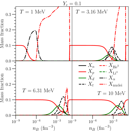

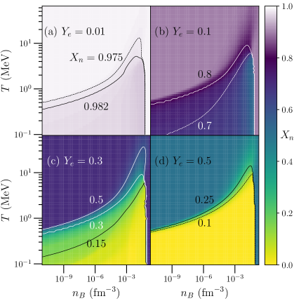
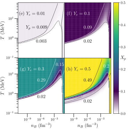
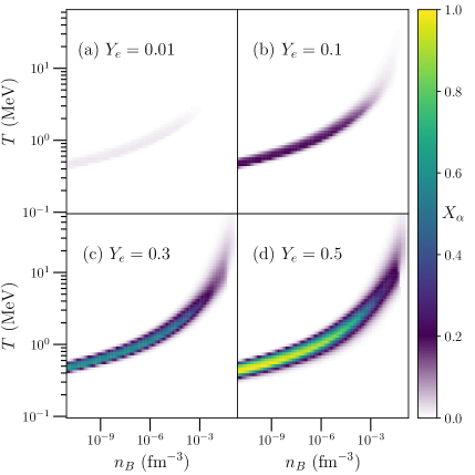
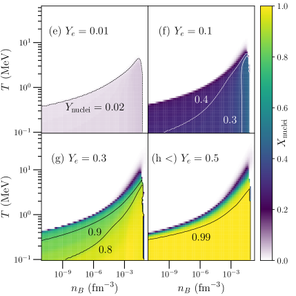
Fig. 2 shows baryon number fractions , and Fig. 3 shows baryon number fractions , as a function of baryon density and temperature. Near and at low temperatures, the system consists almost entirely of heavy nuclei. As the temperature increases, the non-uniform clusters transform to uniform matter. On the other hand, as decreases, nuclei are replaced by free neutrons. The critical temperature of the gas-liquid phase transition is around several to tens of MeV depending on the proton fraction.
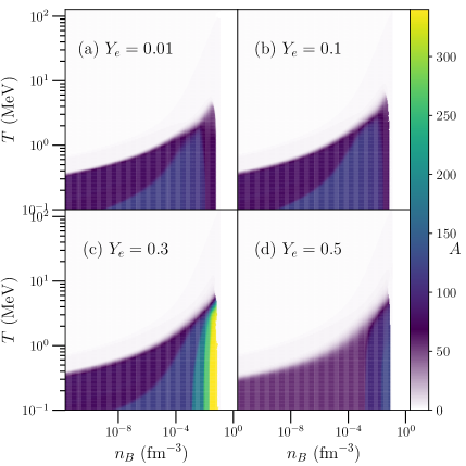
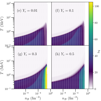
To compute the average proton and neutron number of nuclei, we define
| (53) |
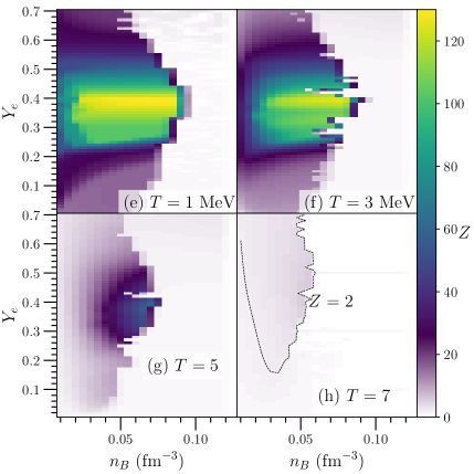
where this sum includes the light nuclei , , , and . We define a similar quantity , and the average nuclear mass number is then . Fig. 4 shows and as a function of baryon density and temperature. The maximum A for our EOS is limited to about 340. For symmetric nuclear matter, reaches the upper limit we set. For smaller electron fractions, the maximum mass number decreases to 120 as neutrons leave nuclei to form a gas. The shell structure of nuclei is evident in the figures as rapid color changes. As baryon density increases, rises to several plateaus. Fig. 5 shows the charge and mass number of nuclei as a function of density and electron fraction at four fixed temperatures. The transition density from inhomogeneous matter to homogeneous matter is not independent of proton fraction, as observed in microscopic calculations of the equation of state Fiorilla et al. (2012); Wellenhofer et al. (2015). The transition density is largest near , which is to be expected since heavy laboratory nuclei have a similar proton fraction. At higher temperatures nuclei disappear as we approach the liquid gas transition.
III.2 Comparison with other EOSs
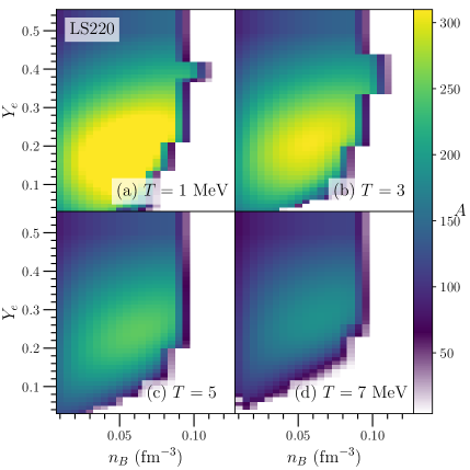
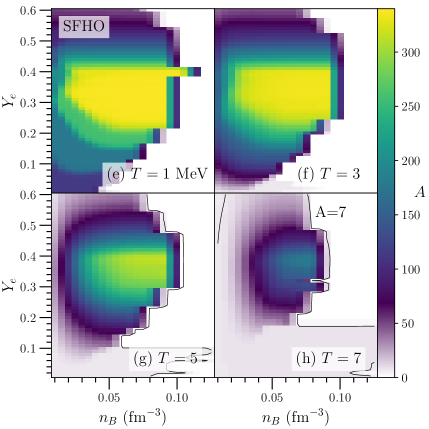
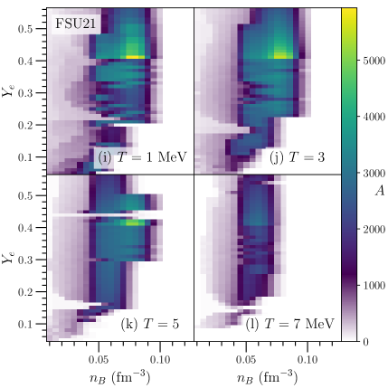
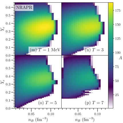
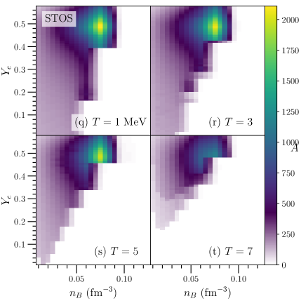
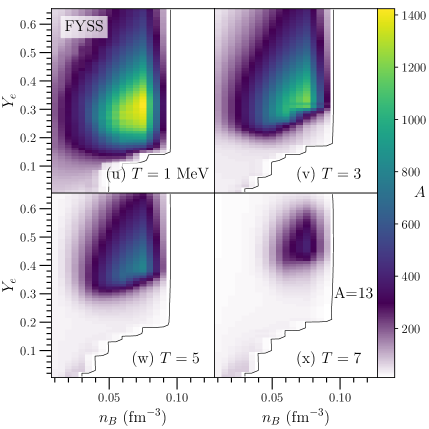
Fig. 6 shows the average mass number as a function of baryon density and temperature for several other EOSs: LS220 Lattimer and Swesty (1991), SFHO Steiner et al. (2013), FSU21 Shen et al. (2011), NRAPR Schneider et al. (2019a), STOS Shen et al. (1998), and FYSS Furusawa et al. (2011). Note that these results were interpolated from the files created by Ref. O'Connor and Ott (2010) (and stored at stellarcollapse.org), and thus details may differ slightly from the original files. Significant differences can be found among these plots for the predictions of mass number in inhomogeneous phase. The plots fall into two categories. STOS, FSU21 and FYSS allow nuclei with maximum mass number around several thousand, while LS220, NRAPR and SFHo limit A below several hundred. There is also some variation between models in the dependence of the phase transition between nuclei and nuclear matter. In FSU21 and FYSS, the phase transition is nearly -independent. Note that different panels have different maximum values of , and this impacts the apparent shape of the transition to nucleonic matter. The STOS, FSU21, and FYSS tables all include a pasta phase before transitioning to homogeneous matter, and this also complicates the comparison. The inclusion of the pasta phase, in general, decreases binding energy and therefore favors a late transition to homogeneous matter. Note however that the difference of the mass number between EOS tables does not strongly impact the thermodynamic quantities such as the pressure and entropy Burrows and Lattimer (1984).
III.3 Nuclear distribution
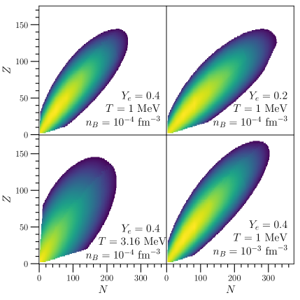
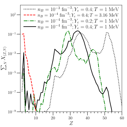
Fig. 7 shows the nuclear distribution for selected points in the EOS as in Shen et al. (2010). Our results are similar, and our restriction of and is evident in the linear cutoff in the distribution near the lower-left corner in each panel. A significant number of nuclei participate in the EOS at each point. Even though we do not fully explore this uncertainty in this work, we find that changing the distribution can significantly change the transition to nucleonic matter. This variation may impact core-collapse supernovae and protoneutron star evolution, as implied by the recent discussion in Ref. Roggero et al. (2018). Fig. 8 shows the isotopic distribution for the same four points in the space. The distribution shows a structure created by the magic numbers (peaks near Z=28 and Z=50 are evident), as well as a peak at low Z as found earlier in Ref. Souza et al. (2009).
III.4 Monte Carlo results
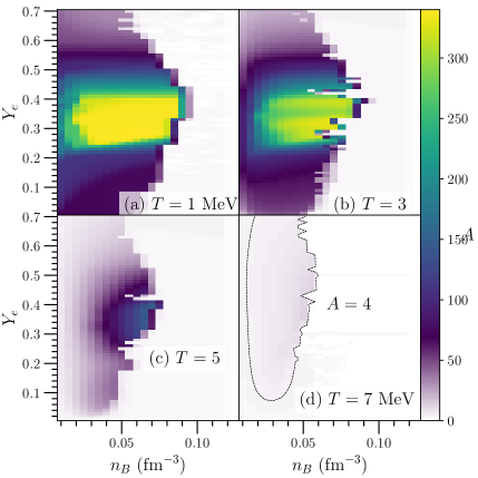
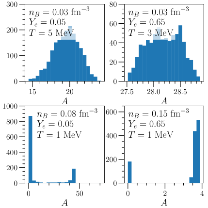
Fig. 9 shows four Monte Carlo plots of the average mass number for some selected points when the seven parameters in our EOS are randomly selected. The distribution gives uncertainty of the EOS in subnuclear density at low temperature at four points where the distribution is nearly maximal. The distribution of A is wider at extreme values of , the top panels show results for and . The bottom-left panel shows that the probability distribution is particularly wide for larger densities near the transition to nucleonic matter in large part because heavy nuclei are present in some models but not others. This effect persists even up to large densities, as shown in the lower-right panel, where nuclei are present for some models but not others.
At some points in the space, the variation shown in Fig. 9 is much smaller than the variation between other EOS tables. At , and MeV (corresponding to the upper-left panel of Fig. 9), LS220 gives but STOS gives whereas our result is . Our variation in some regions, however, is larger than the variation between EOS tables. At , and MeV (corresponding to the lower-left panel of Fig. 9), NRAPR gives , FSU21 gives , FYSS gives , LS220 gives , SFHO gives , and STOS gives , while our result is as large as for some parameterizations.
IV Discussion
While we have created a code which can propagate the uncertainties in the nucleon-nucleon interaction to the resulting equation of state, we have not yet fully included all of the uncertainties. In particular, in addition to the several uncertainties which are involved in the calculation of homogeneous nucleonic matter (discussed in Ref. Du et al. (2019)), there are several additional uncertainties involving nuclei which we have not included. Pasta structures, which are present to surprisingly large temperatures, are not included in the present work. In addition, the modification of the nuclear surface energy due to the presence of nucleons outside nuclei (see, e.g., Refs. Lattimer et al. (1985); Steiner et al. (2005) has not been included in this work. While these corrections are principally important at lower temperatures, and are thus subleading, they may impact the resulting nuclear distribution, particularly in core-collapse supernovae.
One important consideration is the recent experimental measurement of a large value for , as measured in PREX-II Adhikari et al. (2021); Reed et al. (2021). While our fiducial model has a smaller value of one of our alternate parameterizations has a value of MeV, only 6 MeV away from the central value suggested in Ref. Reed et al. (2021).
The nucleon effective mass has been recently shown to be particularly important for both core-collapse supernovae and mergers Andersen et al. (2021); Raithel et al. (2021). While the parameterizations tabulated in Table I all use the same Skryme model (which has a reduced effective mass of 0.904), the zero temperature effective masses are indeed modified in our full Monte Carlo results presented in Figure 9. We do not vary the finite-temperature effective mass from our Skyrme model, SKm∗, because we do not yet have a probability distribution for the finite temperature part of the EOS, but this work is in progress. The effective mass, unlike the equation of state, is not a quantum mechanical observable (it depends, for example, on the arbitrary demarcation between the kinetic and potential energy). Thus it only has a unique specification in the context of a particular model or class of models. However, the effective mass is important for computing the neutrino mean free path, which is well-defined, and clearly relevant for simulations of supernovae and mergers. Thus the best way to properly assess the impact of the effective mass is construct a probability distribution of both the equation of state and the neutrino opacities together. Work on this direction is also in progress.
Acknowledgements
The work of XD and AWS was supported by DOE SciDAC grant DE-SC0018232 and the DOE Office of Nuclear Physics. The work of JWH is supported by the National Science Foundation under Grant No. PHY1652199 and by the U.S. Department of Energy National Nuclear Security Administration under Grant No. DE-NA0003841. This research used resources of the National Energy Research Scientific Computing Center (NERSC), a U.S. Department of Energy Office of Science User Facility located at Lawrence Berkeley National Laboratory, operated under Contract No. DE-AC02-05CH11231. The open-source code for this work, https://github.com/awsteiner/eos, is built upon O2scl Steiner (2014), GSL, HDF5, and matplotlib Hunter (2007). Tables are available for download at https://neutronstars.utk.edu/code/eos.
References
- Bethe et al. (1979) H. A. Bethe, G. E. Brown, J. Applegate, and J. M. Lattimer, Nucl. Phys. A 324, 487 (1979), URL https://doi.org/10.1016/0375-9474(79)90596-7.
- Sekiguchi et al. (2015) Y. Sekiguchi, K. Kiuchi, K. Kyutoku, and M. Shibata, Phys. Rev. D 91, 064059 (2015), URL https://doi.org/10.1103/PhysRevD.91.064059.
- Kasen et al. (2017) D. Kasen, B. Metzger, J. Barnes, E. Quataert, and E. Ramirez-Ruiz, Nature 551, 80 (2017), ISSN 1476-4687, URL https://doi.org/10.1038/nature24453.
- Hinderer (2008) T. Hinderer, Astrophys. J. 677, 1216 (2008), URL https://doi.org/10.1086/533487.
- Bauswein et al. (2017) A. Bauswein, O. Just, H.-T. Janka, and N. Stergioulas, Astrophys. J. Lett. 850, L34 (2017), URL https://doi.org/10.3847%2F2041-8213%2Faa9994.
- Margalit and Metzger (2017) B. Margalit and B. D. Metzger, Astrophys. J. Lett. 850, L19 (2017), URL https://doi.org/10.3847%2F2041-8213%2Faa991c.
- Radice et al. (2018) D. Radice, A. Perego, F. Zappa, and S. Bernuzzi, Astrophys. J. Lett. 852, L29 (2018), URL https://doi.org/10.3847%2F2041-8213%2Faaa402.
- Rezzolla et al. (2018) L. Rezzolla, E. R. Most, and L. R. Weih, Astrophys. J. Lett. 852, L25 (2018), URL https://doi.org/10.3847%2F2041-8213%2Faaa401.
- Ruiz et al. (2018) M. Ruiz, S. L. Shapiro, and A. Tsokaros, Phys. Rev. D 97, 021501 (2018), URL https://link.aps.org/doi/10.1103/PhysRevD.97.021501.
- Shibata et al. (2017) M. Shibata, S. Fujibayashi, K. Hotokezaka, K. Kiuchi, K. Kyutoku, Y. Sekiguchi, and M. Tanaka, Phys. Rev. D 96, 123012 (2017), URL https://link.aps.org/doi/10.1103/PhysRevD.96.123012.
- Lattimer and Swesty (1991) J. M. Lattimer and F. D. Swesty, Nucl. Phys. A 535, 331 (1991), URL https://doi.org/10.1016/0375-9474(91)90452-C.
- Shen et al. (1998) H. Shen, H. Toki, K. Oyamatsu, and K. Sumiyoshi, Nucl. Phys. A 637, 435 (1998), URL https://doi.org/10.1016/S0375-9474(98)00236-X.
- Burrows and Lattimer (1984) A. Burrows and J. M. Lattimer, Astrophys. J. 285, 294 (1984), URL https://doi.org/10.1086/162505.
- Hix et al. (2003) W. R. Hix, O. E. B. Messer, A. Mezzacappa, M. Liebendörfer, J. Sampaio, K. Langanke, D. J. Dean, and G. Martinez-Pinedo, Phys. Rev. Lett. 91, 201102 (2003), URL https://doi.org/10.1103/PhysRevLett.91.201102.
- Botvina and Mishustin (2005) A. Botvina and I. N. Mishustin, Phys. Rev. C 72, 048801 (2005), URL https://doi.org/10.1103/PhysRevC.72.048801.
- O’Connor et al. (2007) E. O’Connor, D. Gazit, C. J. Horowitz, A. Schwenk, and N. Barnea, Phys. Rev. C 75, 055803 (2007), URL https://doi.org/10.1103/PhysRevC.75.055803.
- Arcones et al. (2008) A. Arcones, G. Martinez-Pinedo, E. O’Connor, A. Schwenk, H.-T. Janka, C. J. Horowitz, and K. Langanke, Phys. Rev. C 78, 015806 (2008), URL https://doi.org/10.1103/PhysRevC.78.015806.
- Souza et al. (2009) S. R. Souza, A. W. Steiner, W. G. Lynch, R. Donangelo, and M. A. Famiano, Astrophys. J. 707, 1495 (2009), URL https://doi.org/10.1088/0004-637X/707/2/1495.
- Shen et al. (2010) G. Shen, C. J. Horowitz, and S. Teige, Phys. Rev. C82, 045802 (2010), eprint 1006.0489, URL https://doi.org/10.1103/PhysRevC.82.045802.
- Todd-Rutel and Piekarewicz (2005) B. G. Todd-Rutel and J. Piekarewicz, Phys. Rev. Lett. 95, 122501 (2005), URL https://doi.org/10.1103/PhysRevLett.95.122501.
- Furusawa et al. (2011) S. Furusawa, S. Yamada, K. Sumiyoshi, and H. Suzuki, Astrophys. J. 738, 178 (2011), URL https://doi.org/10.1088%2F0004-637x%2F738%2F2%2F178.
- Hempel and Schaffner-Bielich (2010) M. Hempel and J. Schaffner-Bielich, Nucl. Phys. A 837, 210 (2010), URL https://doi.org/10.1016/j.nuclphysa.2010.02.010.
- Hempel et al. (2012) M. Hempel, T. Fischer, J. Schaffner-Bielich, and M. Liebendörfer, Astrophys. J. 748, 70 (2012), URL https://doi.org/10.1088/0004-637X/748/1/70.
- Typel et al. (2010) S. Typel, G. Röpke, T. Klähn, D. Blaschke, and H. H. Wolter, Phys. Rev. C 81, 015803 (2010), URL https://doi.org/10.1103/PhysRevC.81.015803.
- Fattoyev et al. (2010) F. J. Fattoyev, C. J. Horowitz, J. Piekarewicz, and G. Shen, Phys. Rev. C 82, 055803 (2010), URL https://doi.org/10.1103/PhysRevC.82.055803.
- Steiner et al. (2013) A. W. Steiner, M. Hempel, and T. Fischer, Astrophys. J. 774, 17 (2013), URL https://doi.org/10.1088/0004-637X/774/1/17.
- Typel et al. (2013) S. Typel, M. Oertel, and T. Klaehn, arXiv:1307.5715 (2013), URL http://compose.obspm.fr/.
- Banik et al. (2014) S. Banik, M. Hempel, and D. Bandyopadhyay, Astrophys. J. Suppl. Ser. 214, 22 (2014), URL https://doi.org/10.1088/0067-0049/214/2/22.
- Schneider et al. (2019a) A. Schneider, L. Roberts, C. Ott, and E. O’Connor, Phys. Rev. C 100, 055802 (2019a), eprint 1906.02009, URL https://doi.org/10.1103/PhysRevC.100.055802.
- Schneider et al. (2019b) A. Schneider, C. Constantinou, B. Muccioli, and M. Prakash, Phys. Rev. C 100, 025803 (2019b), eprint 1901.09652, URL https://doi.org/10.1103/PhysRevC.100.025803.
- Skyrme (1959) T. H. R. Skyrme, Nucl. Phys. 9, 615 (1959), URL https://doi.org/10.1016/0029-5582(58)90345-6.
- Krüger et al. (2013) T. Krüger, I. Tews, K. Hebeler, and A. Schwenk, Phys. Rev. C 88, 025802 (2013), URL https://doi.org/10.1103/PhysRevC.88.025802.
- Du et al. (2019) X. Du, A. W. Steiner, and J. W. Holt, Phys. Rev. C 99, 025803 (2019), eprint 1802.09710, URL https://doi.org/10.1103/PhysRevC.99.025803.
- Horowitz et al. (2012) C. Horowitz, G. Shen, E. O’Connor, and C. D. Ott, Phys. Rev. C 86, 065806 (2012), eprint 1209.3173, URL https://dx.doi.org/10.1103/PhysRevC.86.065806.
- Huth et al. (2021) S. Huth, C. Wellenhofer, and A. Schwenk, Phys. Rev. C 103, 025803 (2021), URL https://link.aps.org/doi/10.1103/PhysRevC.103.025803.
- Fowler et al. (1978) W. A. Fowler, C. A. Engelbrecht, and S. E. Woosley, Astrophys. J. 226, 984 (1978), URL https://doi.org/10.1086/156679.
- Baym et al. (1971) G. Baym, C. Pethick, and P. Sutherland, Astrophys. J. 170, 299 (1971), URL https://doi.org/10.1086/151216.
- Zhang et al. (2018) Z. Zhang, Y. Lim, J. W. Holt, and C. M. Ko, Phys. Lett. B 777, 73 (2018), URL https://doi.org/10.1016/j.physletb.2017.12.012.
- Sammarruca et al. (2015) F. Sammarruca, L. Coraggio, J. Holt, N. Itaco, R. Machleidt, and L. Marcucci, Phys. Rev. C 91, 054311 (2015).
- Wellenhofer et al. (2015) C. Wellenhofer, J. W. Holt, and N. Kaiser, Phys. Rev. C 92, 015801 (2015), URL https://doi.org/10.1103/PhysRevC.92.015801.
- Holt et al. (2013) J. W. Holt, N. Kaiser, G. A. Miller, and W. Weise, Phys. Rev. C 88, 024614 (2013), URL https://doi.org/10.1103/PhysRevC.88.024614.
- Holt et al. (2016) J. W. Holt, N. Kaiser, and G. A. Miller, Phys. Rev. C 93, 064603 (2016), URL https://doi.org/10.1103/PhysRevC.93.064603.
- Constantinou et al. (2014) C. Constantinou, B. Muccioli, M. Prakash, and J. M. Lattimer, Phys. Rev. C89, 065802 (2014), URL https://doi.org/10.1103/PhysRevC.89.065802.
- Rrapaj et al. (2016) E. Rrapaj, A. Roggero, and J. W. Holt, Phys. Rev. C 93, 065801 (2016), URL https://link.aps.org/doi/10.1103/PhysRevC.93.065801.
- Audi et al. (2012) G. Audi, M. Wang, A. Wapstra, F. Kondev, M. MacCormick, X. Xu, and B. Pfeiffer, Chinese Physics C 36, 1287 (2012), URL https://doi.org/10.1088/1674-1137/36/12/002.
- Möller et al. (1995) P. Möller, J. R. Nix, W. D. Myers, and W. J. Swiatecki, Atom. Data Nucl. Data Tabl. 59, 185 (1995), URL https://doi.org/10.1006/adnd.1995.1002.
- Goriely et al. (2007) S. Goriely, M. Samyn, and J. M. Pearson, Phys. Rev. C 75, 064312 (2007), URL https://doi.org/10.1103/PhysRevC.75.064312.
- Steiner et al. (2015) A. W. Steiner, S. Gandolfi, F. J. Fattoyev, and W. G. Newton, Phys. Rev. C 91, 015804 (2015), URL https://doi.org/10.1103/PhysRevC.91.015804.
- Kortelainen et al. (2014) M. Kortelainen, J. McDonnell, W. Nazarewicz, E. Olsen, P.-G. Reinhard, J. Sarich, N. Schunck, S. M. Wild, D. Davesne, J. Erler, et al., Phys. Rev. C 89, 054314 (2014), URL https://doi.org/10.1103/PhysRevC.89.054314.
- Fiorilla et al. (2012) S. Fiorilla, N. Kaiser, and W. Weise, Nucl. Phys. A880, 65 (2012), eprint 1111.2791, URL https://doi.org/10.1016/j.nuclphysa.2012.01.003.
- Shen et al. (2011) G. Shen, C. J. Horowitz, and E. O’Connor, Phys. Rev. C 83, 065808 (2011), URL https://doi.org/10.1103/PhysRevC.83.065808.
- O'Connor and Ott (2010) E. O'Connor and C. D. Ott, Classical and Quantum Gravity 27, 114103 (2010), URL https://doi.org/10.1088/0264-9381/27/11/114103.
- Roggero et al. (2018) A. Roggero, J. Margueron, L. F. Roberts, and S. Reddy, Phys. Rev. C 97, 045804 (2018), URL https://link.aps.org/doi/10.1103/PhysRevC.97.045804.
- Lattimer et al. (1985) J. M. Lattimer, C. J. Pethick, D. G. Ravenhall, and D. Q. Lamb, Nucl. Phys. A 432, 646 (1985), URL https://doi.org/10.1016/0375-9474(85)90006-5.
- Steiner et al. (2005) A. W. Steiner, M. Prakash, J. M. Lattimer, and P. J. Ellis, Phys. Rep. 411, 325 (2005), URL http://doi.org/10.1016/j.physrep.2005.02.004.
- Adhikari et al. (2021) D. Adhikari, H. Albataineh, D. Androic, K. Aniol, D. S. Armstrong, T. Averett, C. Ayerbe Gayoso, S. Barcus, V. Bellini, R. S. Beminiwattha, et al. (PREX Collaboration), Phys. Rev. Lett. 126, 172502 (2021), URL https://link.aps.org/doi/10.1103/PhysRevLett.126.172502.
- Reed et al. (2021) B. T. Reed, F. J. Fattoyev, C. J. Horowitz, and J. Piekarewicz, Phys. Rev. Lett. 126, 172503 (2021), URL https://link.aps.org/doi/10.1103/PhysRevLett.126.172503.
- Andersen et al. (2021) O. E. Andersen, S. Zha, A. da Silva Schneider, A. Betranhandy, S. M. Couch, and E. P. O’Connor, arXiv:2106.09734 (2021), URL https://arxiv.org/abs/2106.09734.
- Raithel et al. (2021) C. Raithel, V. Paschalidis, and F. Özel, arXiv:2104.07226 (2021), URL https://arxiv.org/abs/2104.07226.
- Steiner (2014) A. W. Steiner, O2scl: Object-oriented scientific computing library (2014), Astrophysics Source Code Library, record ascl:1408.019, URL http://ascl.net/1408.019.
- Hunter (2007) J. D. Hunter, Computing in Science & Engineering 9, 90 (2007).