Solving discrete constrained problems on de Rham complex

Abstract

The main difficulty in solving the discrete constrained problem is its poor and even ill condition. In this paper, we transform the discrete constrained problems on de Rham complex to Laplace-like problems. This transformation not only make the constrained problems solvable, but also make it easy to use the existing iterative methods and preconditioning techniques to solving large-scale discrete constrained problems.

Keywords: constrained problem, divergence-free, ill condition, iterative method

1 Introduction

Many systems of partial differential equations contain constraint conditions. For example, when solving the second-order Maxwell equation, we want the solution to satisfy the divergence-free condition $\nabla\cdot\mathbf{u}=0$. To this end, we insert a Lagrange multiplier into the equation

$$\begin{split}\nabla\times\nabla\times\mathbf{u}+c\mathbf{u}+\nabla p&=\mathbf{f},\\ \nabla\cdot\mathbf{u}&=0.\end{split}$$ (1)

Then the component in the solution that dose not satisfy the condition $\nabla\cdot\mathbf{u}=0$ is eliminated. The weak formulation for such problems is

$$\begin{split}a(\mathbf{u},\mathbf{v})+b(\mathbf{v},p)&=(\mathbf{f},\mathbf{v})\,\quad\forall\mathbf{v}\in V,\\ b(\mathbf{u},q)&=0\qquad\quad\forall q\in Q.\end{split}$$ (2)

Here $V$ and $Q$ are the function spaces for $\mathbf{u}$ and $p$, respectively. By constructing two proper finite element spaces $V_{h}$ and $Q_{h}$ for the two spaces, we obtain its discrete problem

$$\begin{split}a(\mathbf{u}_{h},\mathbf{v})+b(\mathbf{v}_{h},p_{h})&=(\mathbf{f},\mathbf{v}_{h})\quad\forall\mathbf{v}_{h}\in V_{h},\\ b(\mathbf{u}_{h},q_{h})&=0\qquad\quad\;\,\forall q_{h}\in Q_{h}.\end{split}$$ (3)

Usually this kind of discrete problems has poor condition. This results in that many existing iterative methods and preconditioning techniques that are efficient for Laplace-like problems are inefficient and even invalid for such problems. With some boundary conditions and domains with some special shapes, we can prove that $\mathbf{u}$ in (2) and $\mathbf{u}_{h}$ in (3) for the mixed Maxwell equation (1) are unique, but the terms $b(\mathbf{u},q)$ in (2) and $b(q_{h},\mathbf{u}_{h})$ in (3) no longer satisfy the inf-sup condition. This makes its discrete system non-invertible. Even direct methods can not solve it. Thing is worse for the constrained grad-div problem

$$\begin{split}-\nabla(\nabla\cdot\mathbf{u})+c\mathbf{u}+\nabla\times\mathbf{p}&=\mathbf{f},\\ \nabla\times\mathbf{u}&=0.\end{split}$$

There is an infinite-dimensional kernel contained in its constraint condition $\nabla\times\mathbf{u}=0$. Its corresponding discrete system is highly ill.

A popular method to deal with such discrete problems is penalty method [4]. If the $\mathbf{u}_{h}$ in (3) is unique, the system of the penalty method is solvable. With the penalty parameter becoming large, the penalty solution tends to the exact solution. If we want more precious solution, the penalty parameter should be larger. However, if the penalty parameter is too large, the condition of the system of penalty method become terrible. Besides this, because of the limited machine precision, the penalty parameter can be arbitrarily large. There are also researches on the preconditioned discretizations for partial differential equations that can match such problems [6].

The Maxwell operator and grad-div operator are the $k=1$ and $k=2$ forms of $d^{*}d$ operator on $\mathbb{R}^{3}$ complex

$$\begin{split}\lx@xy@svg{\hbox{\raise 0.0pt\hbox{\kern 5.5pt\hbox{\ignorespaces\ignorespaces\ignorespaces\hbox{\vtop{\kern 0.0pt\offinterlineskip\halign{\entry@#!@&&\entry@@#!@\cr&&&&&\crcr}}}\ignorespaces{\hbox{\kern-5.5pt\raise 0.0pt\hbox{\hbox{\kern 0.0pt\raise 0.0pt\hbox{\hbox{\kern 3.0pt\raise 0.0pt\hbox{$\textstyle{0\ignorespaces\ignorespaces\ignorespaces\ignorespaces}$}}}}}}}\ignorespaces\ignorespaces\ignorespaces\ignorespaces{}{\hbox{\lx@xy@droprule}}\ignorespaces{\hbox{\kern 29.5pt\raise 0.0pt\hbox{\hbox{\kern 0.0pt\raise 0.0pt\hbox{\lx@xy@tip{1}\lx@xy@tip{-1}}}}}}{\hbox{\lx@xy@droprule}}{\hbox{\lx@xy@droprule}}{\hbox{\kern 29.5pt\raise 0.0pt\hbox{\hbox{\kern 0.0pt\raise 0.0pt\hbox{\hbox{\kern 3.0pt\raise 0.0pt\hbox{$\textstyle{H({\text{grad}})\ignorespaces\ignorespaces\ignorespaces\ignorespaces}$}}}}}}}\ignorespaces\ignorespaces\ignorespaces\ignorespaces{}{\hbox{\lx@xy@droprule}}\ignorespaces\ignorespaces\ignorespaces{\hbox{\kern 77.2639pt\raise 5.39166pt\hbox{{}\hbox{\kern 0.0pt\raise 0.0pt\hbox{\hbox{\kern 3.0pt\hbox{\hbox{\kern 0.0pt\raise-2.39166pt\hbox{$\scriptstyle{\nabla}$}}}\kern 3.0pt}}}}}}\ignorespaces{\hbox{\kern 95.87503pt\raise 0.0pt\hbox{\hbox{\kern 0.0pt\raise 0.0pt\hbox{\lx@xy@tip{1}\lx@xy@tip{-1}}}}}}{\hbox{\lx@xy@droprule}}{\hbox{\lx@xy@droprule}}{\hbox{\kern 95.87503pt\raise 0.0pt\hbox{\hbox{\kern 0.0pt\raise 0.0pt\hbox{\hbox{\kern 3.0pt\raise 0.0pt\hbox{$\textstyle{H({\text{curl}})\ignorespaces\ignorespaces\ignorespaces\ignorespaces}$}}}}}}}\ignorespaces\ignorespaces\ignorespaces\ignorespaces{}{\hbox{\lx@xy@droprule}}\ignorespaces\ignorespaces\ignorespaces{\hbox{\kern 138.06253pt\raise 5.68333pt\hbox{{}\hbox{\kern 0.0pt\raise 0.0pt\hbox{\hbox{\kern 3.0pt\hbox{\hbox{\kern 0.0pt\raise-2.1pt\hbox{$\scriptstyle{\nabla\times}$}}}\kern 3.0pt}}}}}}\ignorespaces{\hbox{\kern 159.47226pt\raise 0.0pt\hbox{\hbox{\kern 0.0pt\raise 0.0pt\hbox{\lx@xy@tip{1}\lx@xy@tip{-1}}}}}}{\hbox{\lx@xy@droprule}}{\hbox{\lx@xy@droprule}}{\hbox{\kern 159.47226pt\raise 0.0pt\hbox{\hbox{\kern 0.0pt\raise 0.0pt\hbox{\hbox{\kern 3.0pt\raise 0.0pt\hbox{$\textstyle{H({\text{div}})\ignorespaces\ignorespaces\ignorespaces\ignorespaces}$}}}}}}}\ignorespaces\ignorespaces\ignorespaces\ignorespaces{}{\hbox{\lx@xy@droprule}}\ignorespaces\ignorespaces\ignorespaces{\hbox{\kern 195.8702pt\raise 5.39166pt\hbox{{}\hbox{\kern 0.0pt\raise 0.0pt\hbox{\hbox{\kern 3.0pt\hbox{\hbox{\kern 0.0pt\raise-2.39166pt\hbox{$\scriptstyle{\nabla\cdot}$}}}\kern 3.0pt}}}}}}\ignorespaces{\hbox{\kern 219.98618pt\raise 0.0pt\hbox{\hbox{\kern 0.0pt\raise 0.0pt\hbox{\lx@xy@tip{1}\lx@xy@tip{-1}}}}}}{\hbox{\lx@xy@droprule}}{\hbox{\lx@xy@droprule}}{\hbox{\kern 219.98618pt\raise 0.0pt\hbox{\hbox{\kern 0.0pt\raise 0.0pt\hbox{\hbox{\kern 3.0pt\raise 0.0pt\hbox{$\textstyle{L^{2}\ignorespaces\ignorespaces\ignorespaces\ignorespaces}$}}}}}}}\ignorespaces\ignorespaces\ignorespaces\ignorespaces{}{\hbox{\lx@xy@droprule}}\ignorespaces{\hbox{\kern 259.59174pt\raise 0.0pt\hbox{\hbox{\kern 0.0pt\raise 0.0pt\hbox{\lx@xy@tip{1}\lx@xy@tip{-1}}}}}}{\hbox{\lx@xy@droprule}}{\hbox{\lx@xy@droprule}}{\hbox{\kern 259.59174pt\raise 0.0pt\hbox{\hbox{\kern 0.0pt\raise 0.0pt\hbox{\hbox{\kern 3.0pt\raise 0.0pt\hbox{$\textstyle{0.}$}}}}}}}\ignorespaces}}}}\ignorespaces\end{split} \textstyle{0\ignorespaces\ignorespaces\ignorespaces\ignorespaces} \textstyle{H({\text{grad}})\ignorespaces\ignorespaces\ignorespaces\ignorespaces} \scriptstyle{\nabla} \textstyle{H({\text{curl}})\ignorespaces\ignorespaces\ignorespaces\ignorespaces} \scriptstyle{\nabla\times} \textstyle{H({\text{div}})\ignorespaces\ignorespaces\ignorespaces\ignorespaces} \scriptstyle{\nabla\cdot} \textstyle{L^{2}\ignorespaces\ignorespaces\ignorespaces\ignorespaces} \textstyle{0.} \textstyle{0\ignorespaces\ignorespaces\ignorespaces\ignorespaces} \textstyle{H({\text{grad}})\ignorespaces\ignorespaces\ignorespaces\ignorespaces} \scriptstyle{\nabla} \textstyle{H({\text{curl}})\ignorespaces\ignorespaces\ignorespaces\ignorespaces} \scriptstyle{\nabla\times} \textstyle{H({\text{div}})\ignorespaces\ignorespaces\ignorespaces\ignorespaces} \scriptstyle{\nabla\cdot} \textstyle{L^{2}\ignorespaces\ignorespaces\ignorespaces\ignorespaces} \textstyle{0.}$$

For the general de Rham complex

$$\begin{split}\lx@xy@svg{\hbox{\raise 0.0pt\hbox{\kern 5.5pt\hbox{\ignorespaces\ignorespaces\ignorespaces\hbox{\vtop{\kern 0.0pt\offinterlineskip\halign{\entry@#!@&&\entry@@#!@\cr&&&&&\crcr}}}\ignorespaces{\hbox{\kern-5.5pt\raise 0.0pt\hbox{\hbox{\kern 0.0pt\raise 0.0pt\hbox{\hbox{\kern 3.0pt\raise 0.0pt\hbox{$\textstyle{0\ignorespaces\ignorespaces\ignorespaces\ignorespaces}$}}}}}}}\ignorespaces\ignorespaces\ignorespaces\ignorespaces{}{\hbox{\lx@xy@droprule}}\ignorespaces{\hbox{\kern 29.5pt\raise 0.0pt\hbox{\hbox{\kern 0.0pt\raise 0.0pt\hbox{\lx@xy@tip{1}\lx@xy@tip{-1}}}}}}{\hbox{\lx@xy@droprule}}{\hbox{\lx@xy@droprule}}{\hbox{\kern 29.5pt\raise 0.0pt\hbox{\hbox{\kern 0.0pt\raise 0.0pt\hbox{\hbox{\kern 3.0pt\raise 0.0pt\hbox{$\textstyle{V^{0}\ignorespaces\ignorespaces\ignorespaces\ignorespaces}$}}}}}}}\ignorespaces\ignorespaces\ignorespaces\ignorespaces{}{\hbox{\lx@xy@droprule}}\ignorespaces\ignorespaces\ignorespaces{\hbox{\kern 52.53386pt\raise 6.075pt\hbox{{}\hbox{\kern 0.0pt\raise 0.0pt\hbox{\hbox{\kern 3.0pt\hbox{\hbox{\kern 0.0pt\raise-3.075pt\hbox{$\scriptstyle{d^{0}}$}}}\kern 3.0pt}}}}}}\ignorespaces{\hbox{\kern 70.35556pt\raise 0.0pt\hbox{\hbox{\kern 0.0pt\raise 0.0pt\hbox{\lx@xy@tip{1}\lx@xy@tip{-1}}}}}}{\hbox{\lx@xy@droprule}}{\hbox{\lx@xy@droprule}}{\hbox{\kern 70.35556pt\raise 0.0pt\hbox{\hbox{\kern 0.0pt\raise 0.0pt\hbox{\hbox{\kern 3.0pt\raise 0.0pt\hbox{$\textstyle{V^{1}\ignorespaces\ignorespaces\ignorespaces\ignorespaces}$}}}}}}}\ignorespaces\ignorespaces\ignorespaces\ignorespaces{}{\hbox{\lx@xy@droprule}}\ignorespaces\ignorespaces\ignorespaces{\hbox{\kern 92.55052pt\raise 6.075pt\hbox{{}\hbox{\kern 0.0pt\raise 0.0pt\hbox{\hbox{\kern 3.0pt\hbox{\hbox{\kern 0.0pt\raise-3.075pt\hbox{$\scriptstyle{d^{1}}$}}}\kern 3.0pt}}}}}}\ignorespaces{\hbox{\kern 111.21112pt\raise 0.0pt\hbox{\hbox{\kern 0.0pt\raise 0.0pt\hbox{\lx@xy@tip{1}\lx@xy@tip{-1}}}}}}{\hbox{\lx@xy@droprule}}{\hbox{\lx@xy@droprule}}{\hbox{\kern 111.21112pt\raise 0.0pt\hbox{\hbox{\kern 0.0pt\raise 0.0pt\hbox{\hbox{\kern 3.0pt\raise 0.0pt\hbox{$\textstyle{\cdots\ignorespaces\ignorespaces\ignorespaces\ignorespaces}$}}}}}}}\ignorespaces\ignorespaces\ignorespaces\ignorespaces{}{\hbox{\lx@xy@droprule}}\ignorespaces\ignorespaces\ignorespaces{\hbox{\kern 130.00151pt\raise 6.075pt\hbox{{}\hbox{\kern 0.0pt\raise 0.0pt\hbox{\hbox{\kern 3.0pt\hbox{\hbox{\kern 0.0pt\raise-3.075pt\hbox{$\scriptstyle{d^{n-1}}$}}}\kern 3.0pt}}}}}}\ignorespaces{\hbox{\kern 148.71112pt\raise 0.0pt\hbox{\hbox{\kern 0.0pt\raise 0.0pt\hbox{\lx@xy@tip{1}\lx@xy@tip{-1}}}}}}{\hbox{\lx@xy@droprule}}{\hbox{\lx@xy@droprule}}{\hbox{\kern 148.71112pt\raise 0.0pt\hbox{\hbox{\kern 0.0pt\raise 0.0pt\hbox{\hbox{\kern 3.0pt\raise 0.0pt\hbox{$\textstyle{V^{n}\ignorespaces\ignorespaces\ignorespaces\ignorespaces}$}}}}}}}\ignorespaces\ignorespaces\ignorespaces\ignorespaces{}{\hbox{\lx@xy@droprule}}\ignorespaces{\hbox{\kern 190.12799pt\raise 0.0pt\hbox{\hbox{\kern 0.0pt\raise 0.0pt\hbox{\lx@xy@tip{1}\lx@xy@tip{-1}}}}}}{\hbox{\lx@xy@droprule}}{\hbox{\lx@xy@droprule}}{\hbox{\kern 190.12799pt\raise 0.0pt\hbox{\hbox{\kern 0.0pt\raise 0.0pt\hbox{\hbox{\kern 3.0pt\raise 0.0pt\hbox{$\textstyle{0,}$}}}}}}}\ignorespaces}}}}\ignorespaces\end{split} \textstyle{0\ignorespaces\ignorespaces\ignorespaces\ignorespaces} \textstyle{V^{0}\ignorespaces\ignorespaces\ignorespaces\ignorespaces} \scriptstyle{d^{0}} \textstyle{V^{1}\ignorespaces\ignorespaces\ignorespaces\ignorespaces} \scriptstyle{d^{1}} \textstyle{\cdots\ignorespaces\ignorespaces\ignorespaces\ignorespaces} \scriptstyle{d^{n-1}} \textstyle{V^{n}\ignorespaces\ignorespaces\ignorespaces\ignorespaces} \textstyle{0,} \textstyle{0\ignorespaces\ignorespaces\ignorespaces\ignorespaces} \textstyle{V^{0}\ignorespaces\ignorespaces\ignorespaces\ignorespaces} \scriptstyle{d^{0}} \textstyle{V^{1}\ignorespaces\ignorespaces\ignorespaces\ignorespaces} \scriptstyle{d^{1}} \textstyle{\cdots\ignorespaces\ignorespaces\ignorespaces\ignorespaces} \scriptstyle{d^{n-1}} \textstyle{V^{n}\ignorespaces\ignorespaces\ignorespaces\ignorespaces} \textstyle{0,}$$

these constrained problems can be written in a uniform formulation

$$\begin{split}(d^{k})^{*}d^{k}\mathbf{u}+c\mathbf{u}+d^{k-1}\mathbf{p}&=\mathbf{f},\\ (d^{k-1})^{*}\mathbf{u}&=\mathbf{g}.\end{split}$$ (4)

In this paper, we study the discrete problem of the constrained problem (4) in the uniform framework of de Rham complex. Using the property of complex, we construct several equivalent problems for the corresponding discrete problem (3) for (4). No mater whether the discrete system (3) is invertible or not, only if the component $\mathbf{u}_{h}$ is unique, we can solve it though some well-posed problems in the equivalent problems that we construct. Furthermore, the spectral distributions of the equations contained in these equivalent problems are Laplace-like. Then it is easy to use many existing iterative methods and preconditioning techniques to solve large-scalar discrete constrained problems.

This paper is organized as follows. We consider the matrix form of the discrete constrained system first. In Section 2, we set up the matrix constrained system and derive some theoretical results that we shall use in the later sections. In Section 3 and Section 4, we construct equivalent problems for the case $\mathbf{g}=0$ and $\mathbf{g}\not=0$ in (4), respectively. In Section 5, we study the discretization of the constrained problems on de Rham complex and illustrate its relationship with the matrix system we studied in previous sections. In Section 6, we consider some problems that are involved in solving the equivalent problems. In Section 7, we take the constrained Maxwell and grad-div problems as numerical examples to verify the equivalent problems we construct. Section 8 are some conclusions.

2 Matrix aspects of the constrained problem

Before we consider the discretization of the constrained problems on de Rham complex, we study its matrix system:

$$\begin{split}(\mathcal{A}+c\mathcal{M})u+\mathcal{B}p&=\mathcal{F},\\ \mathcal{B}^{T}u&=\mathcal{G}.\end{split}$$ (5)

In this section, we definite this matrix system and derive some theoretical results that we shall use in the later sections. In Section 5, we will show the relation between the finite element discretization and this system.

In the system (5), it involves the following matrices and vectors:

Definition 2.1.

Let $N,M$ be two positive integers. Let $\mathcal{A}\in\mathbb{C}^{N\times N}$, $\mathcal{B}\in\mathbb{C}^{N\times M}$, $\mathcal{M}\in\mathbb{C}^{N\times N}$, $\mathcal{F}\in\mathbb{C}^{N\times 1}$, $\mathcal{G}\in\mathbb{C}^{M\times 1}$, $u\in\mathbb{C}^{N\times 1}$, $p\in\mathbb{C}^{M\times 1}$ and $c\geq 0$ be a nonnative real number. Here $\mathcal{A}$ is Hermitian positive semi-definite and $\mathcal{M}$ is Hermitian positive definite.

There is an assumption on $\mathcal{A}$, $\mathcal{M}$ and $\mathcal{B}$.

Assumption 1.

$\mathcal{M}$-complex property:

$$\begin{split}\mathcal{A}\mathcal{M}^{-1}\mathcal{B}=0.\end{split}$$

This is the main difference between the system (5) and general systems with constraint conditions. This property corresponds to the basic property of the operator on complexes. This is the reason that we call this property ’complex’. When solving the system (5), it also involves an extra matrix:

Definition 2.2.

$\mathcal{U}\in\mathbb{C}^{M\times M}$ is a Hermitian positive definite matrix.

We consider the Hermitian generalized eigenvalue problem

$$\begin{split}\mathcal{A}u=\lambda\mathcal{M}u,\\ \end{split}$$ (6)

According to its solutions, the entire space $\mathbb{C}^{N}$ can be divided into two $\mathcal{M}$-orthogonal parts:

$$\begin{split}\mathbb{C}^{N}=\mathbb{C}_{1}\oplus_{\mathcal{M}}{\text{Ker}}\mathcal{A}.\end{split}$$

Here $\mathbb{C}_{1}$ is spanned by the eigenvectors of the nonzero eigenvalues of (6). The set of nonzero eigenpairs of (6) is denoted by

$$\begin{split}\left\{\left(\lambda^{(1)}_{i},\mathfrak{u}^{(1)}_{i}\right)\right\}_{i=1}^{\dim\mathbb{C}_{1}}.\end{split}$$ (7)

The set

$$\begin{split}\left\{\mathfrak{u}^{(1)}_{i}\right\}_{i=1}^{\dim\mathbb{C}_{1}}.\end{split}$$ (8)

can be a base of the subspace $\mathbb{C}_{1}$. Similar to (6), for the Hermitian generalized eigenvalue problem

$$\begin{split}\mathcal{B}\mathcal{U}\mathcal{B}^{T}u=\lambda\mathcal{M}u,\end{split}$$ (9)

there is another $\mathcal{M}$-orthogonal decomposition for $\mathbb{C}^{N}$:

$$\begin{split}\mathbb{C}^{N}=\mathbb{C}_{2}\oplus_{\mathcal{M}}{\text{Ker}}\mathcal{B}\mathcal{U}\mathcal{B}^{T},\end{split}$$

where $\mathbb{C}_{2}$ is spanned by the eigenvectors of the nonzero eigenvalues of (9). The set of nonzero eigenpairs of (9) is denoted by

$$\begin{split}\left\{\left(\lambda^{(2)}_{i},\mathfrak{u}^{(2)}_{i}\right)\right\}_{i=1}^{\dim\mathbb{C}_{2}}.\end{split}$$ (10)

The set

$$\begin{split}\left\{\mathfrak{u}^{(2)}_{i}\right\}_{i=1}^{\dim\mathbb{C}_{2}}.\end{split}$$ (11)

can be a base of the subspace $\mathbb{C}_{2}$.

For an eigenpair $\left(\lambda^{(2)}_{i},\mathfrak{u}^{(2)}_{i}\right)$ in the set (10), we have

$$\begin{split}\frac{1}{\lambda^{(2)}_{i}}\mathcal{M}^{-1}\mathcal{B}\mathcal{U}\mathcal{B}^{T}\mathfrak{u}^{(2)}_{i}=\mathfrak{u}^{(2)}_{i}.\end{split}$$

By Assumption 1, we have

$$\begin{split}\mathcal{A}\mathfrak{u}^{(2)}_{i}=\frac{1}{\lambda^{(2)}_{i}}\mathcal{M}^{-1}\mathcal{A}\mathcal{B}\mathcal{U}\mathcal{B}^{T}\mathfrak{u}^{(2)}_{i}=0,\end{split}$$

and we obtain

$$\begin{split}\mathfrak{u}^{(2)}_{i}\in{\text{Ker}}\mathcal{A}.\end{split}$$

As the set (11) is a base of $\mathbb{C}_{2}$, we have

$$\begin{split}\mathbb{C}_{2}\subset{\text{Ker}}\mathcal{A}.\end{split}$$

We denote the intersection of ${\text{Ker}}\mathcal{A}$ and ${\text{Ker}}\mathcal{B}\mathcal{U}\mathcal{B}^{T}$ by

$$\begin{split}\mathbb{C}_{0}\triangleq{\text{Ker}}\mathcal{A}\cap{\text{Ker}}\mathcal{B}\mathcal{U}\mathcal{B}^{T}.\end{split}$$

The $\mathbb{C}_{0}$ is the eigenspace of the zero eigenvalue of the generalized eigenvalue problem

$$\begin{split}\left(\mathcal{A}+\mathcal{B}\mathcal{U}\mathcal{B}^{T}\right)u=\lambda\mathcal{M}u.\end{split}$$ (12)

Then the entire space $\mathbb{C}^{N}$ can be decomposed into three $\mathcal{M}$-orthogonal parts:

$$\begin{split}\mathbb{C}^{N}=\mathbb{C}_{0}\oplus_{\mathcal{M}}\mathbb{C}_{1}\oplus_{\mathcal{M}}\mathbb{C}_{2}.\end{split}$$ (13)

Consequently, there is a $\mathcal{M}^{-1}$-orthogonal decomposition for $\mathbb{C}^{N}$:

$$\begin{split}\mathbb{C}^{N}=\mathcal{M}\mathbb{C}_{0}\oplus_{\mathcal{M}^{-1}}\mathcal{M}\mathbb{C}_{1}\oplus_{\mathcal{M}^{-1}}\mathcal{M}\mathbb{C}_{2}.\end{split}$$

The two kernels can be presented by

$$\begin{split}{\text{Ker}}\mathcal{A}=\mathbb{C}_{0}\oplus_{\mathcal{M}}\mathbb{C}_{2}\quad\text{and}\quad{\text{Ker}}\mathcal{B}\mathcal{U}\mathcal{B}^{T}=\mathbb{C}_{0}\oplus_{\mathcal{M}}\mathbb{C}_{1}.\end{split}$$ (14)

Definition 2.3.

The set $\left\{\mathfrak{u}^{(0)}_{i}\right\}_{i=1}^{\dim\mathbb{C}_{0}}$ is a $\mathcal{M}$-orthogonal base of the subspace $\mathbb{C}_{0}$. There is $\mathfrak{u}^{(0)T}_{i}\mathcal{M}\mathfrak{u}^{(0)}_{i}=1$ for $i=1,\cdots,\dim\mathbb{C}_{0}$. The matrix $\mathcal{H}\in\mathbb{C}^{N\times\dim\mathbb{C}_{0}}$ is constructed by this base $\mathcal{H}=\left[\mathfrak{u}^{(0)}_{1},\mathfrak{u}^{(0)}_{2},\cdots,\mathfrak{u}^{(0)}_{\dim\mathbb{C}_{0}}\right]$.

The set $\left\{\mathfrak{u}^{(0)}_{i}\right\}_{i=1}^{\dim\mathbb{C}_{0}}$ can be gotten through computing the eigenvectors of zero eigenvalue in the eigenvalue problem (12). We consider the generalized eigenvalue problem

$$\begin{split}\mathcal{M}\mathcal{H}\mathcal{H}^{T}\mathcal{M}u=\lambda\mathcal{M}u.\end{split}$$ (15)

By Definition 2.3, for a $\mathfrak{u}^{(0)}_{i}$ in the set $\left\{\mathfrak{u}^{(0)}_{i}\right\}_{i=1}^{\dim\mathbb{C}_{0}}$, we have

$$\begin{split}\mathcal{M}\mathcal{H}\mathcal{H}^{T}\mathcal{M}\mathfrak{u}^{(0)}_{i}=\left(u^{(0)T}_{i}\mathcal{M}\mathfrak{u}^{(0)}_{i}\right)\mathcal{M}\mathfrak{u}^{(0)}_{i}=\mathcal{M}u^{(0)}_{i}.\end{split}$$

Then the set of nonzero eigenpairs of (15) is

$$\begin{split}\left\{\left(1,\mathfrak{u}^{(0)}_{i}\right)\right\}_{i=1}^{\dim\mathbb{C}_{0}}.\end{split}$$ (16)

By the $\mathcal{M}$-orthogonal decomposition (13), we know

$$\begin{split}{\text{Ker}}\mathcal{M}\mathcal{H}\mathcal{H}^{T}\mathcal{M}=\mathbb{C}_{1}\oplus_{\mathcal{M}}\mathbb{C}_{2}.\end{split}$$

Summarizing the matrix operators and the subspaces, we have the following theorem.

Theorem 2.4.

$$\begin{split}\mathcal{A}\mathbb{C}_{0}&=\{0\},\qquad\qquad\qquad\mathcal{A}\mathbb{C}_{2}=\mathcal{M}\mathbb{C}_{1},\qquad\qquad\mathcal{A}\mathbb{C}_{2}=\{0\},\\ \mathcal{B}\mathcal{U}\mathcal{B}^{T}\mathbb{C}_{0}&=\{0\},\qquad\qquad\mathcal{B}\mathcal{U}\mathcal{B}^{T}\mathbb{C}_{2}=\{0\},\qquad\quad\mathcal{B}\mathcal{U}\mathcal{B}^{T}\mathbb{C}_{2}=\mathcal{M}\mathbb{C}_{2},\\ \mathcal{M}\mathcal{H}\mathcal{H}^{T}\mathcal{M}\mathbb{C}_{0}&=\mathcal{M}\mathbb{C}_{0},\quad\,\mathcal{M}\mathcal{H}\mathcal{H}^{T}\mathcal{M}\mathbb{C}_{2}=\{0\},\quad\mathcal{M}\mathcal{H}\mathcal{H}^{T}\mathcal{M}\mathbb{C}_{2}=\{0\}.\end{split}$$

Theorem 2.5.

Let $c\geq 0$. For $f^{(1)}\in\mathbb{C}_{1}$, there a unique solution $u^{(1)}$ in the subspace $\mathbb{C}_{1}$ satisfying $\mathcal{A}u^{(1)}+c\mathcal{M}u^{(1)}=\mathcal{M}f^{(1)}$. For $f^{(2)}\in\mathbb{C}_{2}$, there a unique solution $u^{(2)}$ in the subspace $\mathbb{C}_{2}$ satisfying $\mathcal{B}^{T}\mathcal{U}\mathcal{B}u^{(2)}+c\mathcal{M}u^{(2)}=\mathcal{M}f^{(2)}$. For $f^{(0)}\in\mathbb{C}_{0}$, there a unique solution $u^{(0)}$ in the subspace $\mathbb{C}_{0}$ satisfying $\mathcal{M}\mathcal{H}\mathcal{H}^{T}\mathcal{M}u^{(0)}=\mathcal{M}f^{(0)}$.

Proof.

As $\mathcal{A}$ is positive semi-definite, the eigenvalues in the nonzero eigenpair set (7) are all positive. As $f^{(1)}\in\mathbb{C}_{1}$, using the base (8), it can be expanded as

$$\begin{split}f^{(1)}=\sum_{i=1}^{\dim\mathbb{C}_{1}}f^{(1)}_{i}\mathfrak{u}^{(1)}_{i}.\end{split}$$ (17)

Here $f^{(1)}_{i}\in\mathbb{C}$ is the coefficient of each eigenvector in the base (8). Similarly, $u^{(1)}\in\mathbb{C}_{1}$ can be expanded as

$$\begin{split}u^{(1)}=\sum_{i=1}^{\dim\mathbb{C}_{1}}u^{(1)}_{i}\mathfrak{u}^{(1)}_{i},\end{split}$$ (18)

where $u^{(1)}_{i}\in\mathbb{C}$ is the coefficient to be computed.

Putting the expansions (17) and (18) into the equation, we have

$$\begin{split}\left(\mathcal{A}+c\mathcal{M}\right)\sum_{i=1}^{\dim\mathbb{C}_{1}}u^{(1)}_{i}\mathfrak{u}^{(1)}_{i}=\mathcal{M}\sum_{i=1}^{\dim\mathbb{C}_{1}}f^{(1)}_{i}\mathfrak{u}^{(1)}_{i}.\end{split}$$

By the equation $\mathcal{A}\mathfrak{u}^{(1)}_{i}=\lambda^{(1)}_{i}\mathcal{M}\mathfrak{u}^{(1)}_{i}$, we have

$$\begin{split}\sum_{i=1}^{\dim\mathbb{C}_{1}}\left(\lambda^{(1)}_{i}+c\right)u^{(1)}_{i}\mathcal{M}\mathfrak{u}^{(1)}_{i}=\sum_{i=1}^{\dim\mathbb{C}_{1}}f^{(1)}_{i}\mathcal{M}\mathfrak{u}^{(1)}_{i}.\end{split}$$

Comparing the coefficients on both sides, we obtain

$$\begin{split}\left(\lambda^{(1)}_{i}+c\right)u^{(1)}_{i}=f^{(1)}_{i}\quad\text{for each }i.\end{split}$$

Then we have

$$\begin{split}u^{(1)}_{i}=\frac{f^{(1)}_{i}}{\lambda^{(1)}_{i}+c}\end{split}$$

and we obtain the unique solution $u^{(1)}\in\mathbb{C}_{1}$ of the equation $\mathcal{A}u^{(1)}+c\mathcal{M}u^{(1)}=\mathcal{M}f^{(1)}$.

The proofs for the following two results are similar. ∎

Theorem 2.6.

${\text{Ker}}\mathcal{B}^{T}={\text{Ker}}\mathcal{B}\mathcal{U}\mathcal{B}^{T}=\mathbb{C}_{0}\oplus_{\mathcal{M}}\mathbb{C}_{1}$.

Proof.

For $u\in{\text{Ker}}\mathcal{B}^{T}$, we have $\mathcal{B}\mathcal{U}\mathcal{B}^{T}u=\mathcal{B}\mathcal{U}(\mathcal{B}^{T}u)=0$ and then $u\in{\text{Ker}}\mathcal{B}\mathcal{U}\mathcal{B}^{T}$.

For $u\in{\text{Ker}}\mathcal{B}\mathcal{U}\mathcal{B}^{T}$, we have

$$\begin{split}\mathcal{B}\mathcal{U}\mathcal{B}^{T}u=0\Longrightarrow u^{T}\mathcal{B}\mathcal{U}\mathcal{B}^{T}u=0\Longrightarrow(\mathcal{B}^{T}u)^{T}\mathcal{U}(\mathcal{B}^{T}u)=0.\end{split}$$

As $\mathcal{U}$ is Hermitian positive definite, we have $\mathcal{B}^{T}u=0$ and then $u\in{\text{Ker}}\mathcal{B}^{T}$. ∎

Theorem 2.7.

$\mathbb{C}^{M}={\text{Ker}}\mathcal{B}\oplus{\text{Im}}\mathcal{B}^{T}$.

Proof.

There is an orthogonal decomposition for $\mathbb{C}^{M}$:

$$\begin{split}\mathbb{C}^{M}={\text{Im}}\mathcal{B}^{T}\oplus\left({\text{Im}}\mathcal{B}^{T}\right)^{\perp}.\end{split}$$ (19)

For $p\in\left({\text{Im}}\mathcal{B}^{T}\right)^{\perp}$, we have

$$\begin{split}(\mathcal{B}p,v)=(p,\mathcal{B}^{T}v)=0\quad\text{for any }v\in\mathbb{C}^{N}.\end{split}$$

Here we use $\mathcal{B}^{T}v\in{\text{Im}}\mathcal{B}^{T}$ for any $v\in\mathbb{C}^{N}$. Then we have $\mathcal{B}p=0$ and $\left({\text{Im}}\mathcal{B}^{T}\right)^{\perp}\subset{\text{Ker}}\mathcal{B}$.

For $p\in{\text{Im}}\mathcal{B}^{T}$, there is a $v\in\mathbb{C}^{N}$ such that $p=\mathcal{B}^{T}v$. For $q\in{\text{Ker}}\mathcal{B}$, we have

$$\begin{split}(p,q)=(\mathcal{B}^{T}v,p)=(v,\mathcal{B}q)=0.\end{split}$$

Then we have ${\text{Ker}}\mathcal{B}\perp{\text{Im}}\mathcal{B}^{T}$. By the decomposition (19), we have ${\text{Ker}}\mathcal{B}\subset\left({\text{Im}}\mathcal{B}^{T}\right)^{\perp}$.

Then we have ${\text{Ker}}\mathcal{B}=\left({\text{Im}}\mathcal{B}^{T}\right)^{\perp}$. By the decomposition (19), we obtain the conclusion. ∎

With the similar proof, we have the following theorem.

Theorem 2.8.

$\mathbb{C}^{N}={\text{Ker}}\mathcal{B}^{T}\oplus{\text{Im}}\mathcal{B}$.

Theorem 2.9.

$\mathbb{C}_{2}={\text{Im}}\mathcal{M}^{-1}\mathcal{B}$ and $\mathcal{M}\mathbb{C}_{2}={\text{Im}}\mathcal{B}$.

Proof.

By Theorem 2.8, we have

$$\begin{split}\mathbb{C}^{N}={\text{Ker}}\mathcal{B}^{T}\oplus{\text{Im}}\mathcal{B}={\text{Ker}}\mathcal{B}^{T}\oplus_{\mathcal{M}}\mathcal{M}^{-1}{\text{Im}}\mathcal{B}={\text{Ker}}\mathcal{B}^{T}\oplus_{\mathcal{M}}{\text{Im}}\mathcal{M}^{-1}\mathcal{B}.\end{split}$$

By Theorem 2.6, we have

$$\begin{split}{\text{Ker}}\mathcal{B}^{T}={\text{Ker}}\mathcal{B}\mathcal{U}\mathcal{B}^{T}=\mathbb{C}_{0}\oplus_{\mathcal{M}}\mathbb{C}_{1}.\end{split}$$

By the $\mathcal{M}$-decomposition for $\mathbb{C}^{N}$ (13), we obtain $\mathbb{C}_{2}={\text{Im}}\mathcal{M}^{-1}\mathcal{B}$.

The second result $\mathcal{M}\mathbb{C}_{2}={\text{Im}}\mathcal{B}$ is equivalent to the first one. ∎

Theorem 2.10.

For $\mathcal{G}\in{\text{Im}}\mathcal{B}^{T}$, if there is a $u\in\mathbb{C}^{N}$ such that $\mathcal{B}\mathcal{U}\mathcal{B}^{T}u=\mathcal{B}\mathcal{U}\mathcal{G}$, then $\mathcal{B}^{T}u=\mathcal{G}$.

Proof.

Letting $\tilde{\mathcal{G}}=\mathcal{B}^{T}u_{g}$, then we have $\tilde{\mathcal{G}}\in{\text{Im}}\mathcal{B}^{T}$ and $\mathcal{B}\mathcal{U}\mathcal{B}^{T}u_{g}=\mathcal{B}\mathcal{U}\tilde{\mathcal{G}}$. Consequently, we have $\mathcal{G}-\tilde{\mathcal{G}}\in{\text{Im}}\mathcal{B}^{T}$ and $\mathcal{B}\mathcal{U}(\mathcal{G}-\tilde{\mathcal{G}})=0$. Then $\mathcal{U}(\mathcal{G}-\tilde{\mathcal{G}})\in{\text{Ker}}\mathcal{B}$. As ${\text{Ker}}\mathcal{B}\perp{\text{Im}}\mathcal{B}^{T}$ by Theorem 2.7, we have $(\mathcal{G}-\tilde{\mathcal{G}})^{T}\mathcal{U}(\mathcal{G}-\tilde{\mathcal{G}})=0$. As $\mathcal{U}$ is a Hermitian positive definite matrix, we have $\mathcal{G}-\tilde{\mathcal{G}}=0$. ∎

3 The case $\mathcal{G}=0$

In this section, we consider the solution of (5) in the case $\mathcal{G}=0$:

$$\begin{split}(\mathcal{A}+c\mathcal{M})u+\mathcal{B}p&=\mathcal{F},\\ \mathcal{B}^{T}u&=0.\end{split}$$ (20)

3.1 The case $\dim\mathbb{C}_{0}=0$

In this case, the subspace $\mathbb{C}_{0}$ vanishes. The $\mathcal{M}$-orthogonal decomposition (13) for $\mathbb{C}^{N}$ becomes

$$\begin{split}\mathbb{C}^{N}=\mathbb{C}_{1}\oplus_{\mathcal{M}}\mathbb{C}_{2}.\end{split}$$ (21)

The vector $\mathcal{M}^{-1}\mathcal{F}$ can be divided into two $\mathcal{M}$- orthogonal parts:

$$\begin{split}\mathcal{M}^{-1}\mathcal{F}\triangleq f^{(1)}+f^{(2)}.\end{split}$$ (22)

Here $f^{(1)}\in\mathbb{C}_{1}$ and $f^{(2)}\in\mathbb{C}_{2}$. Consequently, the term $\mathcal{F}$ can be divided into two $\mathcal{M}^{-1}$- orthogonal parts:

$$\begin{split}\mathcal{F}=\mathcal{M}f^{(1)}+\mathcal{M}f^{(2)},\end{split}$$

where $\mathcal{M}f^{(1)}\in\mathcal{M}\mathbb{C}_{1}$ and $\mathcal{M}f^{(2)}\in\mathcal{M}\mathbb{C}_{2}$.

By the constraint condition $\mathcal{B}^{T}u=0$ in the system (20), we know that $u\in{\text{Ker}}\mathcal{B}^{T}$. As $\dim\mathbb{C}_{0}=0$, by Theorem 2.6, we have

$$\begin{split}{\text{Ker}}\mathcal{B}=\mathbb{C}_{1}.\end{split}$$

Then the solution $u\in\mathbb{C}^{N}$ in the system (20) can be written as

$$\begin{split}u\triangleq u^{(1)},\end{split}$$ (23)

where $u^{(1)}\in\mathbb{C}_{1}$. Putting the decompositions (22) and (23) into the first equation of (20), we have

$$\begin{split}(\mathcal{A}+c\mathcal{M})u+\mathcal{B}p&=\mathcal{F},\\ (\mathcal{A}+c\mathcal{M})u^{(1)}+\mathcal{B}p&=\mathcal{M}f^{(1)}+\mathcal{M}f^{(2)},\\ \underbrace{(\mathcal{A}+c\mathcal{M})u^{(1)}-\mathcal{M}f^{(1)}}_{\mathcal{M}\mathbb{C}_{1}}&=\underbrace{\mathcal{M}f^{(2)}-\mathcal{B}p}_{\mathcal{M}\mathbb{C}_{2}}.\end{split}$$ (24)

By Theorem 2.4 and $\mathcal{B}p\in{\text{Im}}\mathcal{B}=\mathcal{M}\mathbb{C}_{2}$ in Theorem 2.9, we know that the two parts in the equation above belong to two $\mathcal{M}^{-1}$-orthogonal parts, respectively. Then, to make this equation hold, both parts should be zero. By Theorem 2.5, there is a unique solution $u^{(1)}\in\mathbb{C}_{1}$ satisfying

$$\begin{split}(\mathcal{A}+c\mathcal{M})u^{(1)}=\mathcal{M}f^{(1)}.\end{split}$$

Then by decomposition (23), the solution of $u\in\mathbb{C}^{N}$ in the system (20) is unique in the case $\dim\mathbb{C}_{0}=0$. By Theorem 2.9, there exists a $p\in\mathbb{C}^{M}$ such that

$$\begin{split}\mathcal{B}p=\mathcal{M}f^{(2)}.\end{split}$$ (25)

If the kernel ${\text{Ker}}\mathcal{B}$ in Theorem 2.7 is not trivial or in other words, the columns of $\mathcal{B}$ are not full-rank, $p$ in (20) is not unique.

We consider the equation

$$\begin{split}(\mathcal{A}+\mathcal{B}\mathcal{U}\mathcal{B}^{T})\tilde{u}=\mathcal{F}.\end{split}$$ (26)

As the subspace $\mathbb{C}_{0}$ vanishes, this equation is well-posed and has a unique solution. We divide $\tilde{u}$ into two $\mathcal{M}$-orthogonal parts

$$\begin{split}\tilde{u}\triangleq\tilde{u}^{(1)}+\tilde{u}^{(2)},\end{split}$$ (27)

where $\tilde{u}^{(1)}\in\mathbb{C}_{1}$ and $\tilde{u}^{(2)}\in\mathbb{C}_{2}$. Putting the decompositions (22) and (27) into the equation (26), we have

$$\begin{split}(\mathcal{A}+\mathcal{B}\mathcal{U}\mathcal{B}^{T})\tilde{u}&=\mathcal{F},\\ (\mathcal{A}+\mathcal{B}\mathcal{U}\mathcal{B}^{T})\left(\tilde{u}^{(1)}+\tilde{u}^{(2)}\right)&=\mathcal{M}f^{(1)}+\mathcal{M}f^{(2)},\\ \underbrace{\mathcal{A}\tilde{u}^{(1)}-\mathcal{M}f^{(1)}}_{\mathcal{M}\mathbb{C}_{1}}&=\underbrace{\mathcal{B}\mathcal{U}\mathcal{B}^{T}\tilde{u}^{(2)}-\mathcal{M}f^{(2)}}_{\mathcal{M}\mathbb{C}_{2}}.\end{split}$$

By Theorem 2.4, we know that the two parts in the equation above belong to two $\mathcal{M}^{-1}$-orthogonal parts, respectively. Then, to make this equation hold, both parts should be zero. By Theorem 2.5, $\tilde{u}^{(1)}\in\mathbb{C}_{1}$ and $\tilde{u}^{(2)}\in\mathbb{C}_{2}$ are the unique solutions of $\mathcal{A}\tilde{u}^{(1)}=\mathcal{M}f^{(1)}$ and $\mathcal{B}\mathcal{U}\mathcal{B}^{T}\tilde{u}^{(2)}=\mathcal{M}f^{(2)}$, respectively. Then if we have the solution $\tilde{u}$ of the equation (26), we can obtain the explicit decomposition for the right hand side $\mathcal{F}$:

$$\begin{split}\mathcal{M}f^{(1)}&\equiv\mathcal{A}\tilde{u}^{(1)}=\mathcal{A}\tilde{u},\\ \mathcal{M}f^{(2)}&\equiv\mathcal{B}\mathcal{U}\mathcal{B}^{T}\tilde{u}^{(2)}=\mathcal{B}\mathcal{U}\mathcal{B}^{T}\tilde{u}.\end{split}$$ (28)

Remark 3.1.

If we have the solution $\tilde{u}$ of the equation (26), let $p=\mathcal{U}\mathcal{B}^{T}\tilde{u}$. By the explicit decomposition (28), this $p$ satisfies $\mathcal{B}p=\mathcal{M}f^{(2)}$ in (25). Then we obtain a solution of $p$ for the system (20).

Next, we consider the equation

$$\begin{split}(\mathcal{A}+\mathcal{B}\mathcal{U}\mathcal{B}^{T}+c\mathcal{M})\bar{u}=\mathcal{F}-\mathcal{B}\mathcal{U}\mathcal{B}^{T}\tilde{u}.\end{split}$$ (29)

We divide $\tilde{u}$ into two $\mathcal{M}$-orthogonal parts

$$\begin{split}\bar{u}\triangleq\bar{u}^{(1)}+\bar{u}^{(2)},\end{split}$$ (30)

where $\bar{u}^{(1)}\in\mathbb{C}_{1}$ and $\bar{u}^{(2)}\in\mathbb{C}_{2}$. Putting the decompositions (22) and (30) into the equation (29), we have

$$\begin{split}(\mathcal{A}+\mathcal{B}\mathcal{U}\mathcal{B}^{T}+c\mathcal{M})\bar{u}&=\mathcal{F}-\mathcal{B}\mathcal{U}\mathcal{B}^{T}\tilde{u},\\ (\mathcal{A}+\mathcal{B}\mathcal{U}\mathcal{B}^{T}+c\mathcal{M})\left(\bar{u}^{(1)}+\bar{u}^{(2)}\right)&=\mathcal{M}f^{(1)},\\ \underbrace{(\mathcal{A}+c\mathcal{M})\bar{u}^{(1)}-\mathcal{M}f^{(1)}}_{\mathcal{M}\mathbb{C}_{1}}&=\underbrace{-(\mathcal{B}\mathcal{U}\mathcal{B}^{T}+c\mathcal{M})\bar{u}^{(2)}}_{\mathcal{M}\mathbb{C}_{2}}.\end{split}$$ (31)

By Theorem 2.5, the $\bar{u}^{(1)}\in\mathbb{C}_{1}$ is the unique solution of $(\mathcal{A}+c\mathcal{M})\bar{u}^{(1)}=\mathcal{M}f^{(1)}$ and the $\bar{u}^{(2)}=0\in\mathbb{C}_{2}$ is the unique solution of $(\mathcal{B}\mathcal{U}\mathcal{B}^{T}+c\mathcal{M})\bar{u}^{(2)}=0$. Then combining with the decomposition (30), we obtain the unique solution $\bar{u}$ of the equation (29).

If we compare each component in the solution $\bar{u}$ of (31) and the solution $u$ of (24), we can find that

$$\begin{split}\bar{u}=u.\end{split}$$

Then the solution of $u\in\mathbb{C}^{N}$ in the system (20) can be obtained through solving the two equations (26) and (29). We summarize the two equations as an equivalent problem for the solution $u\in\mathbb{C}^{N}$ in the system (20):

$$\boxed{\begin{split}&\text{If $\dim\mathbb{C}_{0}=0$, solve $\tilde{u}\in\mathbb{C}^{N}$ such that }\\ &\qquad(\mathcal{A}+\mathcal{B}\mathcal{U}\mathcal{B}^{T})\tilde{u}=\mathcal{F},\\ &\text{then solve $u\in\mathbb{C}^{N}$ such that}\\ &\quad(\mathcal{A}+\mathcal{B}\mathcal{U}\mathcal{B}^{T}+c\mathcal{M})u=\mathcal{F}-\mathcal{B}\mathcal{U}\mathcal{B}^{T}\tilde{u}.\\ \end{split}}$$ (32)

For the case $\dim\mathbb{C}_{0}=0$ and $c>0$, we consider the equation

$$\begin{split}(\mathcal{A}+c\mathcal{M})\hat{u}=\mathcal{F}-\mathcal{B}\mathcal{U}\mathcal{B}^{T}\tilde{u}.\end{split}$$ (33)

We divide $\hat{u}$ into two $\mathcal{M}$-orthogonal parts

$$\begin{split}\hat{u}\triangleq\hat{u}^{(1)}+\hat{u}^{(2)},\end{split}$$ (34)

where $\hat{u}^{(1)}\in\mathbb{C}_{1}$ and $\hat{u}^{(2)}\in\mathbb{C}_{2}$. Putting the decompositions (22) and (34) into the equation (33), we have

$$\begin{split}(\mathcal{A}+c\mathcal{M})\hat{u}&=\mathcal{F}-\mathcal{B}\mathcal{U}\mathcal{B}^{T}\tilde{u},\\ (\mathcal{A}+c\mathcal{M})\left(\hat{u}^{(1)}+\hat{u}^{(2)}\right)&=\mathcal{M}f^{(1)},\\ \underbrace{(\mathcal{A}+c\mathcal{M})\hat{u}^{(1)}-\mathcal{M}f^{(1)}}_{\mathcal{M}\mathbb{C}_{1}}&=\underbrace{-c\mathcal{M}\hat{u}^{(2)}}_{\mathcal{M}\mathbb{C}_{2}}.\end{split}$$

By Theorem 2.5, the $\hat{u}^{(1)}\in\mathbb{C}_{1}$ is the unique solution of $(\mathcal{A}+c\mathcal{M})\hat{u}^{(1)}=\mathcal{M}f^{(1)}$. As $\mathcal{M}$ is full-rank. the $\hat{u}^{(2)}=0\in\mathbb{C}_{2}$ is the unique solution of $c\mathcal{M}\hat{u}^{(2)}=0$. If we compare the component in the solution $\hat{u}$ of (35) and the solution $u$ of (24), we can find that

$$\begin{split}\hat{u}=u.\end{split}$$ (35)

Then we have another equivalent problem for the solution $u\in\mathbb{C}^{N}$ in the system (20):

$$\boxed{\begin{split}&\text{If $\dim\mathbb{C}_{0}=0$ and $c>0$,}\\ &\text{ solve $\tilde{u}\in\mathbb{C}^{N}$ such that }\\ &\qquad(\mathcal{A}+\mathcal{B}\mathcal{U}\mathcal{B}^{T})\tilde{u}=\mathcal{F},\\ &\text{ then solve $u\in\mathbb{C}^{N}$ such that}\\ &\quad(\mathcal{A}+c\mathcal{M})u=\mathcal{F}-\mathcal{B}\mathcal{U}\mathcal{B}^{T}\tilde{u}.\\ \end{split}}$$ (36)

Remark 3.2.

If we use direct method, the equation (33) is a little easier to solve than the equation (29) as the equation (29) has more nonzero entries because of the term $\mathcal{B}\mathcal{U}\mathcal{B}^{T}$. When using iterative methods, the equation (29) may be better than the equation (33), especially for large-scalar problems, which we have discussed in our paper [5].

When $c=0$ in this case $\dim\mathbb{C}_{0}=0$, we can construct another equivalent problem for the system (20). By Theorem 2.5, let $u^{(1)}$ be the unique solution in the subspace $\mathbb{C}_{1}$ of the equation $\mathcal{A}u^{(1)}=\mathcal{M}f^{(1)}$ and $u^{(2)}$ be the unique solution in the subspace $\mathbb{C}_{2}$ of the equation $\mathcal{B}\mathcal{U}\mathcal{B}^{T}u^{(2)}=\mathcal{M}f^{(2)}$. The $u=u^{(1)}$ in the unique solution in the system (20) in the case $\dim\mathbb{C}_{0}=0$ and $c=0$. Then for a positive number $\alpha_{1}>0$, we can verify that

$$\begin{split}u_{1}\triangleq u^{(1)}+\frac{1}{\alpha_{1}}u^{(2)}\\ \end{split}$$ (37)

is the unique solution of the equation

$$\begin{split}(\mathcal{A}+\alpha_{1}\mathcal{B}\mathcal{U}\mathcal{B}^{T})u_{1}&=\mathcal{F},\\ (\mathcal{A}+\alpha_{1}\mathcal{B}\mathcal{U}\mathcal{B}^{T})(u^{(1)}+\frac{1}{\alpha_{1}}u^{(2)})&=\mathcal{M}f^{(1)}+\mathcal{M}f^{(2)},\\ \underbrace{\mathcal{A}u^{(1)}-\mathcal{M}f^{(1)}}_{\mathcal{M}\mathbb{C}_{1}}&=\underbrace{\mathcal{M}f^{(2)}-\mathcal{B}\mathcal{U}\mathcal{B}^{T}u^{(2)}}_{\mathcal{M}\mathbb{C}_{2}}.\end{split}$$ (38)

Similarly, for another positive number $\alpha_{2}\not=\alpha_{1}$, we know that

$$\begin{split}u_{2}\triangleq u^{(1)}+\frac{1}{\alpha_{2}}u^{(2)}\end{split}$$ (39)

is the solution of the equation

$$\begin{split}(\mathcal{A}+\alpha_{2}\mathcal{B}\mathcal{U}\mathcal{B}^{T})u_{2}=\mathcal{F}.\end{split}$$ (40)

By combining $u_{1}$ in (37) and $u_{2}$ in (39), we can obtain the solution $u\in\mathbb{C}^{N}$ in the system (20) by

$$\begin{split}u\equiv u^{(1)}=\frac{\alpha_{1}u_{1}-\alpha_{2}u_{2}}{\alpha_{1}-\alpha_{2}}.\end{split}$$

Then in the case $\dim\mathbb{C}_{0}=0$ and $c=0$, the solution $u\in\mathbb{C}^{N}$ in the system (20) can be obtained through the two equations (38) and (40):

$$\boxed{\begin{split}&\text{If $\dim\mathbb{C}_{0}=0$ and $c=0$,}\\ &\text{ solve $u_{1},u_{2}\in\mathbb{C}^{N}$ such that}\\ &\qquad\left(\mathcal{A}+\alpha_{1}\mathcal{B}^{T}\mathcal{U}\mathcal{B}\right)u_{1}=\mathcal{F}\quad\text{ and }\\ &\qquad\left(\mathcal{A}+\alpha_{2}\mathcal{B}^{T}\mathcal{U}\mathcal{B}\right)u_{2}=\mathcal{F},\\ &\text{ then the solution is}\\ &\qquad\qquad u=\frac{\alpha_{1}u_{1}-\alpha_{2}u_{2}}{\alpha_{1}-\alpha_{2}}.\end{split}}$$ (41)

Remark 3.3.

The equivalent problems (32) and (41) are mathematically equivalent in the case $\dim\mathbb{C}_{0}=0$ and $c=0$. The difference is that the last equation in (32) depends on the first solution, while the two equations in (41) are independent. When using iterative methods, two equations in (41) can be solved simultaneously.

3.2 The case $\dim\mathbb{C}_{0}\not=0$ and $c>0$

In this case, the subspace $\mathbb{C}_{0}$ is not trivial. According to the decomposition (13), the vector $\mathcal{M}^{-1}\mathcal{F}$ can be divided into three $\mathcal{M}$-orthogonal parts

$$\begin{split}\mathcal{M}^{-1}\mathcal{F}\triangleq f^{(0)}+f^{(1)}+f^{(2)},\end{split}$$

where $f^{(0)}\in\mathbb{C}_{0}$, $f^{(1)}\in\mathbb{C}_{1}$ and $f^{(2)}\in\mathbb{C}_{2}$. Then there is a $\mathcal{M}^{-1}$-orthogonal decomposition for $\mathcal{F}$

$$\begin{split}\mathcal{F}=\mathcal{M}f^{(0)}+\mathcal{M}f^{(1)}+\mathcal{M}f^{(2)},\end{split}$$ (42)

where $\mathcal{M}f^{(0)}\in\mathcal{M}\mathbb{C}_{0}$, $\mathcal{M}f^{(1)}\in\mathcal{M}\mathbb{C}_{1}$ and $\mathcal{M}f^{(2)}\in\mathcal{M}\mathbb{C}_{2}$.

From the constraint condition $\mathcal{B}^{T}u=0$ in the system (20) and by Theorem 2.6, we know that

$$\begin{split}u\in{\text{Ker}}\mathcal{B}^{T}=\mathbb{C}_{0}\oplus_{\mathcal{M}}\mathbb{C}_{1}.\end{split}$$ (43)

Then the solution of $u\in\mathbb{C}^{N}$ in the system (20) can be divided into two $\mathcal{M}$-orthogonal parts

$$\begin{split}u\triangleq u^{(0)}+u^{(1)},\end{split}$$ (44)

where $u^{(0)}\in\mathbb{C}_{0}$ and $u^{(1)}\in\mathbb{C}_{1}$. Putting the decompositions (42) and (44) into the first equation of the system (20), we have

$$\begin{split}(\mathcal{A}+c\mathcal{M})u+\mathcal{B}p&=\mathcal{F},\\ (\mathcal{A}+c\mathcal{M})(u^{(0)}+u^{(1)})+\mathcal{B}p&=\mathcal{M}{f^{(0)}+\mathcal{M}f^{(1)}+\mathcal{M}f^{(2)}},\\ \underbrace{c\mathcal{M}u^{(0)}-\mathcal{M}f^{(0)}}_{\mathcal{M}\mathbb{C}_{0}}+\underbrace{(\mathcal{A}+c\mathcal{M})u^{(1)}-\mathcal{M}f^{(1)}}_{\mathcal{M}\mathbb{C}_{1}}&=\underbrace{\mathcal{M}f^{(2)}-\mathcal{B}p}_{\mathcal{M}\mathbb{C}_{2}}.\end{split}$$ (45)

By Theorem 2.4 and $\mathcal{B}p\in{\text{Im}}\mathcal{B}=\mathcal{M}\mathbb{C}_{2}$ in Theorem 2.9, we know that the three parts in the equation above belong to three $\mathcal{M}^{-1}$-orthogonal parts, respectively. Then, to make this equation hold, all the three parts should be zero. By Theorem 2.5, there is a unique solution $u^{(1)}\in\mathbb{C}_{1}$ satisfying

$$\begin{split}(\mathcal{A}+c\mathcal{M})u^{(1)}=\mathcal{M}f^{(1)}.\end{split}$$

As $\mathcal{M}$ is full-rank,

$$\begin{split}u^{(2)}=\frac{1}{c}f^{(2)}\end{split}$$

is the unique solution of the equation

$$\begin{split}c\mathcal{M}u^{(0)}-\mathcal{M}f^{(0)}=0.\end{split}$$

Then by the decomposition (44), the solution of $u\in\mathbb{C}^{N}$ in the system (20) is unique in the case $\dim\mathbb{C}_{0}\not=0$ and $c>0$. By Theorem 2.9, there exists a $p\in\mathbb{C}^{M}$ such that

$$\begin{split}\mathcal{B}p=\mathcal{M}f^{(2)}.\end{split}$$ (46)

We compute the eigenvectors of the zero eigenvalue of the generalized eigenvalue problem

$$\begin{split}(\mathcal{A}+\mathcal{B}\mathcal{U}\mathcal{B}^{T})u=\lambda\mathcal{M}u.\end{split}$$ (47)

The eigenvectors of the zero eigenvalue can form a base $\left\{\mathfrak{u}^{(0)}_{1}\right\}_{i=1}^{\dim\mathbb{C}_{0}}$ of the subspace $\mathbb{C}_{0}$ that satisfies Definition 2.3. Let $\mathcal{H}\in\mathbb{C}^{N\times\dim\mathbb{C}_{0}}$:

$$\begin{split}\mathcal{H}=\left[\mathfrak{u}^{(0)}_{1},\mathfrak{u}^{(0)}_{2},\cdots,\mathfrak{u}^{(0)}_{\dim\mathbb{C}_{0}}\right].\end{split}$$

We consider the following equation

$$\begin{split}\left(\mathcal{A}+\mathcal{B}\mathcal{U}\mathcal{B}^{T}+\mathcal{M}\mathcal{H}\mathcal{H}^{T}\mathcal{M}\right)\tilde{u}=\mathcal{F}.\end{split}$$ (48)

We divide $\tilde{u}$ into three $\mathcal{M}$-orthogonal parts

$$\begin{split}\tilde{u}\triangleq\tilde{u}^{(0)}+\tilde{u}^{(1)}+\tilde{u}^{(2)},\end{split}$$ (49)

where $\tilde{u}^{(0)}\in\mathbb{C}_{0}$, $\tilde{u}^{(1)}\in\mathbb{C}_{1}$ and $\tilde{u}^{(2)}\in\mathbb{C}_{2}$. Putting the decompositions (42) and (49) into the equation (48), we have

$$\begin{split}\left(\mathcal{A}+\mathcal{B}\mathcal{U}\mathcal{B}^{T}+\mathcal{M}\mathcal{H}\mathcal{H}^{T}\mathcal{M}\right)\tilde{u}&=\mathcal{F}\\ \left(\mathcal{A}+\mathcal{B}\mathcal{U}\mathcal{B}^{T}+\mathcal{M}\mathcal{H}\mathcal{H}^{T}\mathcal{M}\right)\left(\tilde{u}^{(0)}+\tilde{u}^{(1)}+\tilde{u}^{(2)}\right)&=\mathcal{M}f^{(0)}+\mathcal{M}f^{(1)}+\mathcal{M}f^{(2)}\\ \mathcal{A}\tilde{u}^{(1)}+\mathcal{B}\mathcal{U}\mathcal{B}^{T}\tilde{u}^{(2)}+\mathcal{M}\mathcal{H}\mathcal{H}^{T}\mathcal{M}\tilde{u}^{(0)}&=\mathcal{M}f^{(0)}+\mathcal{M}f^{(1)}+\mathcal{M}f^{(2)}\\ \underbrace{\mathcal{M}\mathcal{H}\mathcal{H}^{T}\mathcal{M}\tilde{u}^{(0)}-\mathcal{M}f^{(0)}}_{\mathcal{M}\mathbb{C}_{0}}+\underbrace{\mathcal{A}\tilde{u}^{(1)}-\mathcal{M}f^{(1)}}_{\mathcal{M}\mathbb{C}_{1}}&=\underbrace{\mathcal{B}\mathcal{U}\mathcal{B}^{T}\tilde{u}^{(2)}-\mathcal{M}f^{(2)}}_{\mathcal{M}\mathbb{C}_{2}}.\end{split}$$

By Theorem 2.4, we know that the three parts in the equation above belong to two $\mathcal{M}^{-1}$-orthogonal parts, respectively. Then, to make this equation hold, all the three parts should be zero. By Theorem 2.5, $\tilde{u}^{(0)}\in\mathbb{C}_{0}$ is the unique solution of $\mathcal{M}\mathcal{H}\mathcal{H}^{T}\mathcal{M}\tilde{u}^{(0)}=\mathcal{M}f^{(0)}$, $\tilde{u}^{(1)}\in\mathbb{C}_{1}$ is the unique solution of $\mathcal{A}\tilde{u}^{(1)}=\mathcal{M}f^{(1)}$ and $u^{(2)}\in\mathbb{C}_{2}$ is the unique solution of $\mathcal{B}\mathcal{U}\mathcal{B}^{T}\tilde{u}^{(2)}=\mathcal{M}f^{(2)}$. Similar to (28), if we have the solution $\tilde{u}$ of the equation (48), we can obtain the explicit decomposition for the right hand side $\mathcal{F}$ in the case $\dim\mathbb{C}_{0}\not=0$:

$$\begin{split}\mathcal{M}f^{(0)}&=\mathcal{M}\mathcal{H}\mathcal{H}^{T}\mathcal{M}\tilde{u},\\ \mathcal{M}f^{(1)}&=\mathcal{A}\tilde{u},\\ \mathcal{M}f^{(2)}&=\mathcal{B}\mathcal{U}\mathcal{B}^{T}\tilde{u}.\end{split}$$ (50)

We consider the equation

$$\begin{split}\left(\mathcal{A}+\mathcal{B}\mathcal{U}\mathcal{B}^{T}+c\mathcal{M}\right)\bar{u}=\mathcal{F}-\mathcal{B}\mathcal{U}\mathcal{B}^{T}\tilde{u}.\end{split}$$ (51)

In this equation, by the decomposition (50), the component of the right hand side in $\mathcal{M}\mathbb{C}_{2}$ is eliminated. To study its solution, we also divide $\bar{u}$ in three $\mathcal{M}$-orthogonal parts

$$\begin{split}\bar{u}\triangleq\bar{u}^{(0)}+\bar{u}^{(1)}+\bar{u}^{(2)},\end{split}$$

where $\bar{u}^{(0)}\in\mathbb{C}_{0}$, $\bar{u}^{(1)}\in\mathbb{C}_{1}$ and $\bar{u}^{(2)}\in\mathbb{C}_{2}$. Then we have

$$\begin{split}(\mathcal{A}+\mathcal{B}\mathcal{U}\mathcal{B}^{T}+c\mathcal{M})\hat{u}&=\mathcal{F}-\mathcal{B}\mathcal{U}\mathcal{B}^{T}\tilde{u}\\ (\mathcal{A}+\mathcal{B}\mathcal{U}\mathcal{B}^{T}+c\mathcal{M})\left(\bar{u}^{(0)}+\bar{u}^{(1)}+\bar{u}^{(2)}\right)&=\mathcal{M}f^{(0)}+\mathcal{M}f^{(1)}\\ \underbrace{c\mathcal{M}\bar{u}^{(0)}-\mathcal{M}f^{(0)}}_{\mathcal{M}\mathbb{C}_{0}}+\underbrace{(\mathcal{A}+c\mathcal{M})\bar{u}^{(1)}-\mathcal{M}f^{(1)}}_{\mathcal{M}\mathbb{C}_{1}}&=-\underbrace{(\mathcal{B}\mathcal{U}\mathcal{B}^{T}+c\mathcal{M})\bar{u}^{(2)}}_{\mathcal{M}\mathbb{C}_{2}}.\end{split}$$

To make this equation hold, all the three parts should be zero as before. By Theorem 2.5, $\bar{u}^{(1)}\in\mathbb{C}_{1}$ is the unique solution of the equation

$$\begin{split}(\mathcal{A}+c\mathcal{M})\bar{u}^{(1)}=\mathcal{M}f^{(1)},\end{split}$$

and $\bar{u}^{(1)}=0\in\mathbb{C}_{2}$ is the unique solution of the equation

$$\begin{split}(\mathcal{B}\mathcal{U}\mathcal{B}^{T}+c\mathcal{M})\bar{u}^{(2)}=0.\end{split}$$

As $\mathcal{M}$ is full-rank,

$$\begin{split}\bar{u}^{(0)}=\frac{1}{c}f^{(0)}\end{split}$$

is the unique solution of the equation

$$\begin{split}c\mathcal{M}\hat{u}^{(0)}-\mathcal{M}f^{(0)}=0.\end{split}$$

If we compare each component in the solution $\bar{u}$ of the equation (51) and the solution $u$ of the equation (45), we obtain that

$$\begin{split}\bar{u}=u.\end{split}$$

Then we have an equivalent problem for the solution $u\in\mathbb{C}^{N}$ in the system (20) in the case $\dim\mathbb{C}_{0}\not=0$ and $c>0$:

$$\boxed{\begin{split}&\text{If $\dim\mathbb{C}_{0}\not=0$ and $c>0$,}\\ &\text{ find the eigenvectors $\mathcal{H}$ of the zero eigenvalue}\\ &\qquad\left(\mathcal{A}+\mathcal{B}\mathcal{U}\mathcal{B}^{T}\right)u=\lambda\mathcal{M}u,\\ &\text{ then solve $\tilde{u}\in\mathbb{C}^{N}$ such that }\\ &\qquad\left(\mathcal{A}+\mathcal{B}\mathcal{U}\mathcal{B}^{T}+\mathcal{M}\mathcal{H}\mathcal{H}^{T}\mathcal{M}\right)\tilde{u}=\mathcal{F},\\ &\text{ then solve $u\in\mathbb{C}^{N}$ such that}\\ &\quad\left(\mathcal{A}+\mathcal{B}\mathcal{U}\mathcal{B}^{T}+c\mathcal{M}\right)u=\mathcal{F}-\mathcal{B}\mathcal{U}\mathcal{B}^{T}\tilde{u}.\\ \end{split}}$$ (52)

Remark 3.4.

The subspace $\mathbb{C}_{0}$ is an inherent characteristic of a system. For a system, the eigenvalue problems (47) needs to be computed only once. The matrix $\mathcal{H}$ can be fixed when the right hand side varies.

As the eigenvectors with zero eigenvalue of the eigenvalue problem are usually full vectors, the term $\mathcal{M}\mathcal{H}\mathcal{H}^{T}\mathcal{M}$ is probably a full matrix. This results that if the dimension of the matrix is a litter large, direct methods become inefficient and even impossible when computing the equation (48). Then the alternative choice is to use iterative methods, where the matrix-vector multiplication $\mathcal{M}\mathcal{H}\mathcal{H}^{T}\mathcal{M}u$ can be computed one by one. Thus we avoid dealing with the term $\mathcal{M}\mathcal{H}\mathcal{H}^{T}\mathcal{M}$ in an explicit way.

Similar to (33), as $c>0$, we consider the equation

$$\begin{split}(\mathcal{A}+c\mathcal{M})\hat{u}=&\mathcal{F}-\mathcal{B}\mathcal{U}\mathcal{B}^{T}\tilde{u}.\end{split}$$ (53)

We also divide $\hat{u}\in\mathbb{C}^{N}$ into three $\mathcal{M}$-orthogonal parts

$$\begin{split}\hat{u}\triangleq\hat{u}^{(0)}+\hat{u}^{(1)}+\hat{u}^{(2)},\end{split}$$ (54)

where $\hat{u}^{(0)}\in\mathbb{C}_{0}$, $\hat{u}^{(1)}\in\mathbb{C}_{1}$ and $\hat{u}^{(2)}\in\mathbb{C}_{2}$. Putting the decompositions (42) and (54) into the equation (53), we have

$$\begin{split}(\mathcal{A}+c\mathcal{M})\hat{u}&=\mathcal{F}-\mathcal{B}\mathcal{U}\mathcal{B}^{T}\tilde{u},\\ (\mathcal{A}+c\mathcal{M})\left(\hat{u}^{(0)}+\hat{u}^{(1)}+\hat{u}^{(2)}\right)&=\mathcal{M}f^{(0)}+\mathcal{M}f^{(1)},\\ \underbrace{c\mathcal{M}\hat{u}^{(0)}-\mathcal{M}f^{(0)}}_{\mathcal{M}\mathbb{C}_{0}}+\underbrace{(\mathcal{A}+c\mathcal{M})\hat{u}^{(1)}-\mathcal{M}f^{(1)}}_{\mathcal{M}\mathbb{C}_{1}}&=-\underbrace{c\mathcal{M}\hat{u}^{(2)}}_{\mathcal{M}\mathbb{C}_{2}}.\end{split}$$

To make this equation hold, all the three parts should be zero. By Theorem 2.5, $\hat{u}^{(1)}\in\mathbb{C}_{1}$ is the unique solution of the equation $\left(\mathcal{A}+c\mathcal{M}\right)\hat{u}^{(1)}=\mathcal{M}f^{(1)}$. As $\mathcal{M}$ is full-rank, $\hat{u}^{(0)}=\frac{1}{c}f^{(0)}$ is the unique solution of the equation $c\mathcal{M}\hat{u}^{(0)}-\mathcal{M}f^{(0)}=0$ and $\hat{u}^{(1)}=0\in\mathbb{C}_{2}$ is the unique solution of the equation $c\mathcal{M}\hat{u}^{(2)}=0$. If we compare each component in the solution $\hat{u}$ of the equation (53) and the solution $u$ of the equation (45), we obtain that

$$\begin{split}\hat{u}=u.\end{split}$$

Then we have another equivalent problem for the solution $u\in\mathbb{C}^{N}$ in the system (20) in the case $\dim\mathbb{C}_{0}\not=0$ and $c>0$:

$$\boxed{\begin{split}&\text{If $\dim\mathbb{C}_{0}\not=0$ and $c>0$,}\\ &\text{ find the eigenvectors $\mathcal{H}$ of the zero eigenvalue}\\ &\qquad\left(\mathcal{A}+\mathcal{B}\mathcal{U}\mathcal{B}^{T}\right)u=\lambda\mathcal{M}u,\\ &\text{ then solve $\tilde{u}\in\mathbb{C}^{N}$ such that }\\ &\qquad\left(\mathcal{A}+\mathcal{B}\mathcal{U}\mathcal{B}^{T}+\mathcal{M}\mathcal{H}\mathcal{H}^{T}\mathcal{M}\right)\tilde{u}=\mathcal{F},\\ &\text{ then solve $u\in\mathbb{C}^{N}$ such that}\\ &\quad\left(\mathcal{A}+c\mathcal{M}\right)u=\mathcal{F}-\mathcal{B}\mathcal{U}\mathcal{B}^{T}\tilde{u}.\\ \end{split}}$$ (55)

3.3 The case $\dim\mathbb{C}_{0}\not=0$ and $c=0$

In the case $c=0$, the problem (20) becomes

$$\begin{split}\mathcal{A}u+\mathcal{B}p&=\mathcal{F}\\ \mathcal{B}^{T}u&=0.\end{split}$$ (56)

As $\dim\mathbb{C}_{0}\not=0$, the right hand side $\mathcal{F}\in\mathbb{C}^{N}$ and the solution $u\in\mathbb{C}^{N}$ in this system can be still decomposed as (42) and (44), respectively. Putting the two decompositions into the first equation of the system (56), we have

$$\begin{split}\mathcal{A}u+\mathcal{B}p&=\mathcal{F},\\ \mathcal{A}(u^{(0)}+u^{(1)})+\mathcal{B}p&=\mathcal{M}f^{(0)}+\mathcal{M}f^{(1)}+\mathcal{M}f^{(2)},\\ \underbrace{\left(\mathcal{A}u^{(1)}-\mathcal{M}f^{(1)}\right)}_{\mathcal{M}\mathbb{C}_{1}}+\underbrace{\left(\mathcal{B}p-\mathcal{M}f^{(2)}\right)}_{\mathcal{M}\mathbb{C}_{2}}&=\underbrace{\mathcal{M}f^{(0)}}_{\mathcal{M}\mathbb{C}_{0}}.\end{split}$$

As the three parts in this equation are $\mathcal{M}^{-1}$-orthogonal, if the term $\mathcal{M}f^{(0)}\not=0$, the equation above never hold. If $\mathcal{M}f^{(0)}=0$, there exist $u^{(1)}$ and $p$ that make this equation hold. Here, $u^{(1)}$ is the unique solution of $\mathcal{A}u^{(1)}=\mathcal{M}f^{(1)}$ in $\mathcal{M}\mathbb{C}_{1}$ by Theorem 2.5 and $p$ satisfies $\mathcal{B}p=\mathcal{M}f^{(2)}$ by Theorem 2.9. However, there is no restriction on the component $u^{(0)}$. For any $u^{(0)}\in\mathbb{C}_{0}$, $u=u^{(0)}+u^{(1)}$ is a solution for $u\in\mathbb{C}^{N}$ in the system (56) when $\mathcal{M}f^{(0)}=0$.

In this paper, we shall not consider this case.

3.4 Summary

We summarize the equivalent problems in Table 1 for the solution $u\in\mathbb{C}^{N}$ in the system (20) with different cases.

	$c>0$	$c=0$
$\dim\mathbb{C}_{0}=0$	(32) (36)	(32) (41)
$\dim\mathbb{C}_{0}\not=0$	(52) (55)	no solution or no unique solution

Table 1: The equivalent problems for the solution $u\in\mathbb{C}^{N}$ in the system (20).

4 The case $\mathcal{G}\not=0$

In this section, we consider the general case $\mathcal{G}\not=0$ for the problem

$$\begin{split}(\mathcal{A}+c\mathcal{M})u+\mathcal{B}p&=\mathcal{F},\\ \mathcal{B}^{T}u&=\mathcal{G}.\end{split}$$ (57)

In this case, $\mathcal{G}$ is required to be contained in ${\text{Im}}\mathcal{B}^{T}$, i.e. $\mathcal{G}\in{\text{Im}}\mathcal{B}^{T}$. Otherwise, there is no solution satisfying the constraint condition $\mathcal{B}^{T}u=\mathcal{G}$.

Remark 4.1.

There is a special case that ${\text{Ker}}\mathcal{B}$ vanishes in Theorem 2.7 and ${\text{Im}}\mathcal{B}^{T}=\mathbb{C}^{M}$. Then there always exists a $u\in\mathbb{C}^{N}$ such that $\mathcal{B}^{T}u=\mathcal{G}$ for any $\mathcal{G}\in\mathbb{C}^{M}$.

In the case $0\not=\mathcal{G}\in{\text{Im}}\mathcal{B}^{T}$, if we have a $u_{g}\in\mathbb{C}^{N}$ satisfying

$$\begin{split}\mathcal{B}^{T}u_{g}=\mathcal{G},\end{split}$$ (58)

then the solution $u\in\mathbb{C}^{N}$ in the system (57) can be the superposition of the two components

$$\begin{split}u=u_{0}+u_{g}.\end{split}$$

Here $u_{0}$ is the solution of the system

$$\begin{split}(\mathcal{A}+c\mathcal{M})u_{0}+\mathcal{B}p&=\mathcal{F}-(\mathcal{A}+c\mathcal{M})u_{g},\\ \mathcal{B}^{T}u_{0}&=0.\end{split}$$ (59)

The solution of the system (59) has been considered in the previous section. The remained thing is how to find a $u_{g}\in\mathbb{C}^{N}$ satisfying the constraint condition $\mathcal{B}^{T}u_{g}=\mathcal{G}$.

By Theorem 2.9, we have

$$\begin{split}\mathcal{B}\mathcal{U}\mathcal{G}\in\mathcal{M}\mathbb{C}_{2}.\end{split}$$

We consider the equation

$$\begin{split}(\mathcal{A}+\mathcal{B}\mathcal{U}\mathcal{B}^{T})u_{g}=\mathcal{B}\mathcal{U}\mathcal{G}.\end{split}$$ (60)

We divide $u_{g}$ into three $\mathcal{M}$-orthogonal parts:

$$\begin{split}u_{g}=u_{g}^{(0)}+u_{g}^{(1)}+u_{g}^{(2)},\end{split}$$ (61)

where $u_{g}^{(0)}\in\mathbb{C}_{0}$, $u_{g}^{(1)}\in\mathbb{C}_{1}$ and $u_{g}^{(2)}\in\mathbb{C}_{2}$. Putting the decomposition (61) into the equation (60), we have

$$\begin{split}(\mathcal{A}+\mathcal{B}\mathcal{U}\mathcal{B}^{T})u_{g}&=\mathcal{B}\mathcal{U}\mathcal{G},\\ (\mathcal{A}+\mathcal{B}\mathcal{U}\mathcal{B}^{T})(u_{g}^{(0)}+u_{g}^{(1)}+u_{g}^{(2)})&=\mathcal{B}\mathcal{U}\mathcal{G},\\ \underbrace{\mathcal{A}u_{g}^{(1)}}_{\mathcal{M}\mathbb{C}_{1}}&=\underbrace{\mathcal{B}\mathcal{U}\mathcal{G}-\mathcal{B}\mathcal{U}\mathcal{B}^{T}u_{g}^{(2)}}_{\mathcal{M}\mathbb{C}_{2}}.\end{split}$$

The two parts in the equation above are $\mathcal{M}^{-1}$-orthogonal. To make this equation hold, both parts should be zero. By Theorem 2.5, $u_{g}^{(1)}=0\in\mathbb{C}_{1}$ is the unique solution of the equation $\mathcal{A}u_{g}^{(1)}=0$ and $u_{g}^{(2)}\in\mathbb{C}_{1}$ is the unique solution of the equation

$$\begin{split}\mathcal{B}\mathcal{U}\mathcal{G}-\mathcal{B}\mathcal{U}\mathcal{B}^{T}u_{g}^{(2)}=0.\end{split}$$ (62)

If $\dim\mathbb{C}_{0}=0$, the component $u_{g}^{(0)}$ vanishes. The equation (60) is well-posed and has a unique solution

$$\begin{split}u_{g}=u_{g}^{(2)}.\end{split}$$

If $\dim\mathbb{C}_{0}\not=0$, the solution of the equation (60) is not unique. For any $u_{g}^{(0)}\in\mathbb{C}_{0}$,

$$\begin{split}u_{g}=u_{g}^{(0)}+u_{g}^{(2)}\end{split}$$

is a solution of the equation (60), where $u_{g}^{(2)}$ satisfies the equation (62). As $u_{g}^{(0)}\in{\text{Ker}}\mathcal{B}\mathcal{U}\mathcal{B}^{T}$ by Theorem 2.4, in the both cases, we have

$$\begin{split}\mathcal{B}\mathcal{U}\mathcal{B}^{T}u_{g}=\mathcal{B}\mathcal{U}\mathcal{B}^{T}u_{g}^{(2)}=\mathcal{B}\mathcal{U}\mathcal{G}.\end{split}$$

In both cases, we know that this $u_{g}$ satisfies the constraint condition $\mathcal{B}^{T}u_{g}=\mathcal{G}\in{\text{Im}}\mathcal{B}^{T}$ by Theorem 2.10.

In the case $\dim\mathbb{C}_{0}\not=0$, we have an alternative way to obtain a $u_{g}$. We insert the term $\mathcal{M}\mathcal{H}\mathcal{H}^{T}\mathcal{M}$ into the equation (60) as that in (48) and get the equation

$$\begin{split}\left(\mathcal{A}+\mathcal{B}\mathcal{U}\mathcal{B}^{T}+\mathcal{M}\mathcal{H}\mathcal{H}^{T}\mathcal{M}\right)u_{g}=\mathcal{B}\mathcal{U}\mathcal{G}.\end{split}$$ (63)

Putting the decompositions (61) into this equation, we have

$$\begin{split}\left(\mathcal{A}+\mathcal{B}\mathcal{U}\mathcal{B}^{T}+\mathcal{M}\mathcal{H}\mathcal{H}^{T}\mathcal{M}\right)u_{g}&=\mathcal{B}\mathcal{U}\mathcal{G},\\ \left(\mathcal{A}+\mathcal{B}\mathcal{U}\mathcal{B}^{T}+\mathcal{M}\mathcal{H}\mathcal{H}^{T}\mathcal{M}\right)\left(u_{g}^{(0)}+u_{g}^{(1)}+u_{g}^{(2)}\right)&=\mathcal{B}\mathcal{U}\mathcal{G},\\ \mathcal{A}u_{g}^{(1)}+\mathcal{B}\mathcal{U}\mathcal{B}^{T}u_{g}^{(2)}+\mathcal{M}\mathcal{H}\mathcal{H}^{T}\mathcal{M}u_{g}^{(0)}&=\mathcal{B}\mathcal{U}\mathcal{G},\\ \underbrace{\mathcal{M}\mathcal{H}\mathcal{H}^{T}\mathcal{M}u_{g}^{(0)}}_{\mathcal{M}\mathbb{C}_{0}}+\underbrace{\mathcal{A}u_{g}^{(1)}}_{\mathcal{M}\mathbb{C}_{1}}&=\underbrace{\mathcal{B}\mathcal{U}\mathcal{G}-\mathcal{B}\mathcal{U}\mathcal{B}^{T}u_{g}^{(2)}}_{\mathcal{M}\mathbb{C}_{2}}.\end{split}$$

To make this equation hold, $u_{g}^{(0)}=0\in\mathbb{C}_{0}$, $u_{g}^{(1)}=0\in\mathbb{C}_{1}$ and $u_{g}^{(2)}\in\mathbb{C}_{2}$ are the unique solutions that make the three $\mathcal{M}^{-1}$-orthogonal parts be zero by Theorem 2.5. Then we obtain a unique solution of the equation (63)

$$\begin{split}u_{g}=u_{g}^{(2)}\in\mathbb{C}_{2}.\end{split}$$

This $u_{g}$ also satisfies the constraint condition $\mathcal{B}^{T}u_{g}=\mathcal{G}\in{\text{Im}}\mathcal{B}^{T}$.

Theorem 4.2.

If $u_{g}\in\mathbb{C}_{2}$ such that $\mathcal{B}^{T}u_{g}=\mathcal{G}\in{\text{Im}}\mathcal{B}^{T}$, and the solution $u$ in the system (20) and the solution $u_{0}$ in the system (59) are unique, then we have $u=u_{0}$.

Proof.

As $u_{g}\in\mathbb{C}_{2}$, we have

$$\begin{split}(\mathcal{A}+c\mathcal{M})u_{g}=c\mathcal{M}u_{g}\in\mathcal{M}\mathbb{C}_{2}.\end{split}$$ (64)

By the analysis in (24) and (45), the solutions $u$ in (20) and $u_{0}$ in (59) are decided by the components in the subspaces $\mathcal{M}\mathbb{C}_{0}$ and $\mathcal{M}\mathbb{C}_{1}$ of their right-hand sides, respectively. Compared with the system (20), the additional term in the right-hand side of the system (59) is $c\mathcal{M}u_{g}\in\mathcal{M}\mathbb{C}_{2}$ by (64). This term has no influence on the solution $u_{0}\in\mathbb{C}_{0}\oplus_{\mathcal{M}}\mathbb{C}_{1}$. The components in $\mathbb{C}_{0}\oplus_{\mathcal{M}}\mathbb{C}_{1}$ in the right-hand sides of the two system are the same. Consequently, their solutions $u$ and $u_{0}$ are the same. ∎

In the case $\dim\mathbb{C}_{0}=0$, we use the equation (60) to solve $u_{g}$, while in the case $\dim\mathbb{C}_{0}\not=0$, we use the equation (63) to solve $u_{g}$. The $u_{g}$ is unique in both equations and $u_{g}\in\mathbb{C}_{2}$ satisfying $\mathcal{B}^{T}u_{g}=\mathcal{G}\in{\text{Im}}\mathcal{B}^{T}$. Then, by Theorem 4.2, we can solve $u_{0}$ in the system (59) by the system (20) which is the case $\mathcal{G}=0$. After obtaining its solution, we add the solution $u_{g}$ of the equation (60) or (63) to it. That is the solution of the general case $0\not=\mathcal{G}\in{\text{Im}}\mathcal{B}^{T}$.

To add the term $u_{g}\in\mathbb{C}_{2}$, the last equations in the equivalent problems (32), (36), (52) and (55):

$$\begin{split}\left(\mathcal{A}+c\mathcal{M}\right)u&=\mathcal{F}-\mathcal{B}\mathcal{U}\mathcal{B}^{T}\tilde{u}\\ \text{and}\quad\left(\mathcal{A}+\mathcal{B}\mathcal{U}\mathcal{B}^{T}+c\mathcal{M}\right)u&=\mathcal{F}-\mathcal{B}\mathcal{U}\mathcal{B}^{T}\tilde{u}\end{split}$$

are modified as

$$\begin{split}\left(\mathcal{A}+c\mathcal{M}\right)u&=\mathcal{F}-\mathcal{B}\mathcal{U}\mathcal{B}^{T}\tilde{u}+\left(\mathcal{A}+c\mathcal{M}\right)u_{g}=\mathcal{F}-\mathcal{B}\mathcal{U}\mathcal{B}^{T}\tilde{u}+c\mathcal{M}u_{g}\\ \text{and}\quad\left(\mathcal{A}+\mathcal{B}\mathcal{U}\mathcal{B}^{T}+c\mathcal{M}\right)u&=\mathcal{F}-\mathcal{B}\mathcal{U}\mathcal{B}^{T}\tilde{u}+\left(\mathcal{A}+\mathcal{B}\mathcal{U}\mathcal{B}^{T}+c\mathcal{M}\right)u_{g}=\mathcal{F}-\mathcal{B}\mathcal{U}\mathcal{B}^{T}\tilde{u}+\mathcal{B}\mathcal{U}\mathcal{G}+c\mathcal{M}u_{g}.\end{split}$$

Here we use $\mathcal{B}\mathcal{U}\mathcal{B}^{T}u_{g}=\mathcal{B}\mathcal{U}\mathcal{G}$ and $\mathcal{A}u_{g}=0$ as $u_{g}\in\mathbb{C}_{2}$. Then, based on the the equivalent problems (32), (36), (52) and (55) for the case $\mathcal{G}=0$, the equivalent problems for the solution $u\in\mathbb{C}^{N}$ in the system (57) are the follows, respectively:

$$\boxed{\begin{split}&\text{If $\dim\mathbb{C}_{0}=0$, solve $u_{g}\in\mathbb{C}^{N}$ such that }\\ &\qquad\left(\mathcal{A}+\mathcal{B}\mathcal{U}\mathcal{B}^{T}\right)u_{g}=\mathcal{B}\mathcal{U}\mathcal{G},\\ &\text{ then solve $\tilde{u}\in\mathbb{C}^{N}$ such that}\\ &\qquad\left(\mathcal{A}+\mathcal{B}\mathcal{U}\mathcal{B}^{T}\right)\tilde{u}=\mathcal{F},\\ &\text{ then solve $u\in\mathbb{C}^{N}$ such that}\\ &\left(\mathcal{A}+\mathcal{B}\mathcal{U}\mathcal{B}^{T}+c\mathcal{M}\right)u=\mathcal{F}-\mathcal{B}\mathcal{U}\mathcal{B}^{T}\tilde{u}+\mathcal{B}\mathcal{U}\mathcal{G}+c\mathcal{M}u_{g}.\\ \end{split}}$$ (65)

$$\boxed{\begin{split}&\text{If $\dim\mathbb{C}_{0}=0$ and $c>0$,}\\ &\text{ solve $u_{g}\in\mathbb{C}^{N}$ such that }\\ &\qquad\left(\mathcal{A}+\mathcal{B}\mathcal{U}\mathcal{B}^{T}\right)u_{g}=\mathcal{B}\mathcal{U}\mathcal{G},\\ &\text{ then solve $\tilde{u}\in\mathbb{C}^{N}$ such that}\\ &\qquad\left(\mathcal{A}+\mathcal{B}\mathcal{U}\mathcal{B}^{T}\right)\tilde{u}=\mathcal{F},\\ &\text{ then solve $u\in\mathbb{C}^{N}$ such that}\\ &\left(\mathcal{A}+c\mathcal{M}\right)u=\mathcal{F}-\mathcal{B}\mathcal{U}\mathcal{B}^{T}\tilde{u}+c\mathcal{M}u_{g}.\end{split}}$$ (66)

$$\boxed{\begin{split}&\text{If $\dim\mathbb{C}_{0}\not=0$ and $c>0$,}\\ &\text{ find the eigenvectors $\mathcal{H}$ of the zero eigenvalue}\\ &\qquad\left(\mathcal{A}+\mathcal{B}\mathcal{U}\mathcal{B}^{T}\right)u=\lambda\mathcal{M}u,\\ &\text{ find $u_{g}\in\mathbb{C}^{N}$ such that }\\ &\qquad\left(\mathcal{A}+\mathcal{B}^{T}\mathcal{U}\mathcal{B}+\mathcal{M}\mathcal{H}\mathcal{H}^{T}\mathcal{M}\right)u_{g}=\mathcal{B}\mathcal{U}\mathcal{G},\\ &\text{ then solve $\tilde{u}\in\mathbb{C}^{N}$ such that }\\ &\qquad\left(\mathcal{A}+\mathcal{B}\mathcal{U}\mathcal{B}^{T}+\mathcal{M}\mathcal{H}\mathcal{H}^{T}\mathcal{M}\right)\tilde{u}=\mathcal{F},\\ &\text{ then solve $u\in\mathbb{C}^{N}$ such that}\\ &\left(\mathcal{A}+\mathcal{B}\mathcal{U}\mathcal{B}^{T}+c\mathcal{M}\right)u=\mathcal{F}-\mathcal{B}\mathcal{U}\mathcal{B}^{T}\tilde{u}+\mathcal{B}\mathcal{U}\mathcal{G}+c\mathcal{M}u_{g}.\\ \end{split}}$$ (67)

$$\boxed{\begin{split}&\text{If $\dim\mathbb{C}_{0}\not=0$ and $c>0$,}\\ &\text{ find the eigenvectors $\mathcal{H}$ of the zero eigenvalue}\\ &\qquad\left(\mathcal{A}+\mathcal{B}\mathcal{U}\mathcal{B}^{T}\right)u=\lambda\mathcal{M}u,\\ &\text{ find $u_{g}\in\mathbb{C}^{N}$ such that }\\ &\qquad\left(\mathcal{A}+\mathcal{B}^{T}\mathcal{U}\mathcal{B}+\mathcal{M}\mathcal{H}\mathcal{H}^{T}\mathcal{M}\right)u_{g}=\mathcal{B}\mathcal{U}\mathcal{G},\\ &\text{ then solve $\tilde{u}\in\mathbb{C}^{N}$ such that }\\ &\qquad\left(\mathcal{A}+\mathcal{B}\mathcal{U}\mathcal{B}^{T}+\mathcal{M}\mathcal{H}\mathcal{H}^{T}\mathcal{M}\right)\tilde{u}=\mathcal{F},\\ &\text{ then solve $u\in\mathbb{C}^{N}$ such that}\\ &\left(\mathcal{A}+c\mathcal{M}\right)u=\mathcal{F}-\mathcal{B}\mathcal{U}\mathcal{B}^{T}\tilde{u}+c\mathcal{M}u_{g}.\end{split}}$$ (68)

When $c=0$ in this case $\dim\mathbb{C}_{0}=0$, we find that $u_{g}$ is not necessary in the last equation of the equivalent problem (65). Then the last two equations are enough in the case $\dim\mathbb{C}_{0}=0$ and $c=0$:

$$\boxed{\begin{split}&\text{If $\dim\mathbb{C}_{0}=0$ and $c=0$,}\\ &\text{ solve $\tilde{u}\in\mathbb{C}^{N}$ such that }\\ &\qquad\left(\mathcal{A}+\mathcal{B}\mathcal{U}\mathcal{B}^{T}\right)\tilde{u}=\mathcal{F},\\ &\text{ then solve $u\in\mathbb{C}^{N}$ such that}\\ &\left(\mathcal{A}+\mathcal{B}\mathcal{U}\mathcal{B}^{T}\right)u=\mathcal{F}-\mathcal{B}\mathcal{U}\mathcal{B}^{T}\tilde{u}+\mathcal{B}\mathcal{U}\mathcal{G}.\\ \end{split}}$$ (69)

For the case $\dim\mathbb{C}_{0}=0$ and $c=0$, the equivalent problem (41) for $\mathcal{G}=0$ can be also modified for the general case $0\not=\mathcal{G}\in{\text{Im}}\mathcal{B}^{T}$. The solution $u\in\mathbb{C}^{N}$ in the system (57) is

$$\begin{split}u=u^{(1)}+u_{g}.\end{split}$$ (70)

Here $u^{(1)}\in\mathbb{C}_{1}$ is unique the solution of $\mathcal{A}u^{(1)}=\mathcal{M}f^{(1)}$ and $u_{g}\in\mathbb{C}_{2}$ is unique the solution of $\mathcal{B}\mathcal{U}\mathcal{B}^{T}u_{g}^{(2)}=\mathcal{B}\mathcal{U}\mathcal{G}$. Let $u^{(2)}\in\mathbb{C}_{2}$ denote the unique solution of $\mathcal{B}\mathcal{U}\mathcal{B}^{T}u^{(2)}=\mathcal{M}f^{(2)}$. Then for a positive number $\alpha_{1}>0$, we can verify that

$$\begin{split}u_{1}\triangleq u^{(1)}+u_{g}+\frac{1}{\alpha_{1}}u^{(2)}\\ \end{split}$$ (71)

is the solution of the problem

$$\begin{split}(\mathcal{A}+\alpha_{1}\mathcal{B}\mathcal{U}\mathcal{B}^{T})u_{1}&=\mathcal{F}+\alpha_{1}\mathcal{B}\mathcal{U}\mathcal{G},\\ (\mathcal{A}+\alpha_{1}\mathcal{B}\mathcal{U}\mathcal{B}^{T})(u^{(1)}+u_{g}+\frac{1}{\alpha_{1}}u^{(2)})&=\mathcal{M}f^{(1)}+\mathcal{M}f^{(2)}+\alpha_{1}\mathcal{B}\mathcal{U}\mathcal{G},\\ \underbrace{\mathcal{A}u^{(1)}-\mathcal{M}f^{(1)}}_{\mathcal{M}\mathbb{C}_{1}}&=\underbrace{\left(\mathcal{M}f^{(2)}-\mathcal{B}\mathcal{U}\mathcal{B}^{T}u^{(2)}\right)+\alpha_{1}\left(\mathcal{B}\mathcal{U}\mathcal{G}-\mathcal{B}\mathcal{U}\mathcal{B}^{T}u_{g}\right)}_{\mathcal{M}\mathbb{C}_{2}}.\end{split}$$ (72)

Similarly, we can also verify that

$$\begin{split}u_{2}\triangleq u^{(1)}+u_{g}+\frac{1}{\alpha_{2}}u^{(2)}\\ \end{split}$$ (73)

is the solution of the equation

$$\begin{split}(\mathcal{A}+\alpha_{2}\mathcal{B}\mathcal{U}\mathcal{B}^{T})u_{1}&=\mathcal{F}+\alpha_{2}\mathcal{B}\mathcal{U}\mathcal{G}.\end{split}$$

Finally, we can obtain the solution (70) by the linear combination of the solutions of two equations (71) and (73):

$$\begin{split}u\equiv u^{(1)}+u_{g}=\frac{\alpha_{1}u_{1}-\alpha_{2}u_{2}}{\alpha_{1}-\alpha_{2}}.\end{split}$$

Then we can obtain the following equivalent problem for the solution $u\in\mathbb{C}^{N}$ in the system (57) in the case $\dim\mathbb{C}_{0}=0$ and $c=0$:

$$\boxed{\begin{split}&\text{If $\dim\mathbb{C}_{0}=0$ and $c=0$, for $\alpha_{1}\not=\alpha_{2}>0$,}\\ &\text{ solve $u_{1},u_{2}\in\mathbb{C}^{N}$ such that}\\ &\;\;\left(\mathcal{A}+\alpha_{1}\mathcal{B}\mathcal{U}\mathcal{B}^{T}\right)u_{1}=\mathcal{F}+\alpha_{1}\mathcal{B}\mathcal{U}\mathcal{G}\;\;\text{ and }\\ &\;\;\left(\mathcal{A}+\alpha_{2}\mathcal{B}\mathcal{U}\mathcal{B}^{T}\right)u_{2}=\mathcal{F}+\alpha_{2}\mathcal{B}\mathcal{U}\mathcal{G},\\ &\text{ then the solution is}\\ &\qquad\qquad u=\frac{\alpha_{1}u_{1}-\alpha_{2}u_{2}}{\alpha_{1}-\alpha_{2}}.\end{split}}$$ (74)

In the equivalent problem (69) and (74), there is no need to compute an explicit $u_{g}$.

In the end of this section, we summarize the equivalent problems in Table 2 for the solution $u\in\mathbb{C}^{N}$ in the system (57) with different cases.

	$c>0$	$c=0$
$\dim\mathbb{C}_{0}=0$	(65) (66)	(65) (66) (69) (74)
$\dim\mathbb{C}_{0}\not=0$	(67) (68)	no solution or no unique solution

Table 2: The equivalent problems for the solution $u\in\mathbb{C}^{N}$ in the system (57).

5 The discretization using finite element complexes

In this section, we use the finite element spaces on discrete de Rham complex to discretize the constrained problem

$$\begin{split}(d^{k})^{*}d^{k}\mathbf{u}+c\mathbf{u}+d^{k-1}\mathbf{p}&=\mathbf{f},\\ (d^{k-1})^{*}\mathbf{u}&=\mathbf{g}.\end{split}$$ (75)

We will show the relation between its discrete weak formulation and the matrix system (5). The main results in this section have been proved in [1, 2, 3, 4]. We refer the readers to these references for more details.

5.1 The weak formulation

We study the weak formulation of (75) in the framework of the Hilbert complex. The de Rham complex is a typical example of the Hilbert complex when the operators are differential operators and the spaces are the corresponding function spaces.

Let us consider a Hilbert complex $(W,d)$. The $d^{k}$ is a closed densely defined operator from $W^{k}$ to $W^{k+1}$ and its domain is denoted by $V^{k}$. Then the corresponding domain complex is

$$\begin{split}\lx@xy@svg{\hbox{\raise 0.0pt\hbox{\kern 5.5pt\hbox{\ignorespaces\ignorespaces\ignorespaces\hbox{\vtop{\kern 0.0pt\offinterlineskip\halign{\entry@#!@&&\entry@@#!@\cr&&&&&\crcr}}}\ignorespaces{\hbox{\kern-5.5pt\raise 0.0pt\hbox{\hbox{\kern 0.0pt\raise 0.0pt\hbox{\hbox{\kern 3.0pt\raise 0.0pt\hbox{$\textstyle{0\ignorespaces\ignorespaces\ignorespaces\ignorespaces}$}}}}}}}\ignorespaces\ignorespaces\ignorespaces\ignorespaces{}{\hbox{\lx@xy@droprule}}\ignorespaces{\hbox{\kern 29.5pt\raise 0.0pt\hbox{\hbox{\kern 0.0pt\raise 0.0pt\hbox{\lx@xy@tip{1}\lx@xy@tip{-1}}}}}}{\hbox{\lx@xy@droprule}}{\hbox{\lx@xy@droprule}}{\hbox{\kern 29.5pt\raise 0.0pt\hbox{\hbox{\kern 0.0pt\raise 0.0pt\hbox{\hbox{\kern 3.0pt\raise 0.0pt\hbox{$\textstyle{V^{0}\ignorespaces\ignorespaces\ignorespaces\ignorespaces}$}}}}}}}\ignorespaces\ignorespaces\ignorespaces\ignorespaces{}{\hbox{\lx@xy@droprule}}\ignorespaces\ignorespaces\ignorespaces{\hbox{\kern 52.53386pt\raise 6.075pt\hbox{{}\hbox{\kern 0.0pt\raise 0.0pt\hbox{\hbox{\kern 3.0pt\hbox{\hbox{\kern 0.0pt\raise-3.075pt\hbox{$\scriptstyle{d^{0}}$}}}\kern 3.0pt}}}}}}\ignorespaces{\hbox{\kern 70.35556pt\raise 0.0pt\hbox{\hbox{\kern 0.0pt\raise 0.0pt\hbox{\lx@xy@tip{1}\lx@xy@tip{-1}}}}}}{\hbox{\lx@xy@droprule}}{\hbox{\lx@xy@droprule}}{\hbox{\kern 70.35556pt\raise 0.0pt\hbox{\hbox{\kern 0.0pt\raise 0.0pt\hbox{\hbox{\kern 3.0pt\raise 0.0pt\hbox{$\textstyle{V^{1}\ignorespaces\ignorespaces\ignorespaces\ignorespaces}$}}}}}}}\ignorespaces\ignorespaces\ignorespaces\ignorespaces{}{\hbox{\lx@xy@droprule}}\ignorespaces\ignorespaces\ignorespaces{\hbox{\kern 92.55052pt\raise 6.075pt\hbox{{}\hbox{\kern 0.0pt\raise 0.0pt\hbox{\hbox{\kern 3.0pt\hbox{\hbox{\kern 0.0pt\raise-3.075pt\hbox{$\scriptstyle{d^{1}}$}}}\kern 3.0pt}}}}}}\ignorespaces{\hbox{\kern 111.21112pt\raise 0.0pt\hbox{\hbox{\kern 0.0pt\raise 0.0pt\hbox{\lx@xy@tip{1}\lx@xy@tip{-1}}}}}}{\hbox{\lx@xy@droprule}}{\hbox{\lx@xy@droprule}}{\hbox{\kern 111.21112pt\raise 0.0pt\hbox{\hbox{\kern 0.0pt\raise 0.0pt\hbox{\hbox{\kern 3.0pt\raise 0.0pt\hbox{$\textstyle{\cdots\ignorespaces\ignorespaces\ignorespaces\ignorespaces}$}}}}}}}\ignorespaces\ignorespaces\ignorespaces\ignorespaces{}{\hbox{\lx@xy@droprule}}\ignorespaces\ignorespaces\ignorespaces{\hbox{\kern 130.00151pt\raise 6.075pt\hbox{{}\hbox{\kern 0.0pt\raise 0.0pt\hbox{\hbox{\kern 3.0pt\hbox{\hbox{\kern 0.0pt\raise-3.075pt\hbox{$\scriptstyle{d^{n-1}}$}}}\kern 3.0pt}}}}}}\ignorespaces{\hbox{\kern 148.71112pt\raise 0.0pt\hbox{\hbox{\kern 0.0pt\raise 0.0pt\hbox{\lx@xy@tip{1}\lx@xy@tip{-1}}}}}}{\hbox{\lx@xy@droprule}}{\hbox{\lx@xy@droprule}}{\hbox{\kern 148.71112pt\raise 0.0pt\hbox{\hbox{\kern 0.0pt\raise 0.0pt\hbox{\hbox{\kern 3.0pt\raise 0.0pt\hbox{$\textstyle{V^{n}\ignorespaces\ignorespaces\ignorespaces\ignorespaces}$}}}}}}}\ignorespaces\ignorespaces\ignorespaces\ignorespaces{}{\hbox{\lx@xy@droprule}}\ignorespaces{\hbox{\kern 190.12799pt\raise 0.0pt\hbox{\hbox{\kern 0.0pt\raise 0.0pt\hbox{\lx@xy@tip{1}\lx@xy@tip{-1}}}}}}{\hbox{\lx@xy@droprule}}{\hbox{\lx@xy@droprule}}{\hbox{\kern 190.12799pt\raise 0.0pt\hbox{\hbox{\kern 0.0pt\raise 0.0pt\hbox{\hbox{\kern 3.0pt\raise 0.0pt\hbox{$\textstyle{0.}$}}}}}}}\ignorespaces}}}}\ignorespaces\end{split} \textstyle{0\ignorespaces\ignorespaces\ignorespaces\ignorespaces} \textstyle{V^{0}\ignorespaces\ignorespaces\ignorespaces\ignorespaces} \scriptstyle{d^{0}} \textstyle{V^{1}\ignorespaces\ignorespaces\ignorespaces\ignorespaces} \scriptstyle{d^{1}} \textstyle{\cdots\ignorespaces\ignorespaces\ignorespaces\ignorespaces} \scriptstyle{d^{n-1}} \textstyle{V^{n}\ignorespaces\ignorespaces\ignorespaces\ignorespaces} \textstyle{0.} \textstyle{0\ignorespaces\ignorespaces\ignorespaces\ignorespaces} \textstyle{V^{0}\ignorespaces\ignorespaces\ignorespaces\ignorespaces} \scriptstyle{d^{0}} \textstyle{V^{1}\ignorespaces\ignorespaces\ignorespaces\ignorespaces} \scriptstyle{d^{1}} \textstyle{\cdots\ignorespaces\ignorespaces\ignorespaces\ignorespaces} \scriptstyle{d^{n-1}} \textstyle{V^{n}\ignorespaces\ignorespaces\ignorespaces\ignorespaces} \textstyle{0.}$$ (76)

The adjoint operator of $d^{k}$ is denoted by $(d^{k})^{*}:W^{k+1}\to W^{k}$ and is defined as

$$\begin{split}\left\langle d^{k}\mathbf{u}\,,\,\mathbf{v}\right\rangle=\left\langle\mathbf{u}\,,\,(d^{k})^{*}\mathbf{v}\right\rangle,\end{split}$$

if $\mathbf{u}\in V^{k}$ or $\mathbf{v}\in W^{k+1}$ vanishes near the boundary. Its domain is a dense subset of $W^{k+1}$ and denoted by $V^{*}_{k+1}$. Then we have the dual complex

$$\begin{split}\lx@xy@svg{\hbox{\raise 0.0pt\hbox{\kern 5.5pt\hbox{\ignorespaces\ignorespaces\ignorespaces\hbox{\vtop{\kern 0.0pt\offinterlineskip\halign{\entry@#!@&&\entry@@#!@\cr&&&&&\crcr}}}\ignorespaces{\hbox{\kern-5.5pt\raise 0.0pt\hbox{\hbox{\kern 0.0pt\raise 0.0pt\hbox{\hbox{\kern 3.0pt\raise 0.0pt\hbox{$\textstyle{0\ignorespaces\ignorespaces\ignorespaces\ignorespaces}$}}}}}}}\ignorespaces\ignorespaces\ignorespaces\ignorespaces{}{\hbox{\lx@xy@droprule}}\ignorespaces{\hbox{\kern 29.5pt\raise 0.0pt\hbox{\hbox{\kern 0.0pt\raise 0.0pt\hbox{\lx@xy@tip{1}\lx@xy@tip{-1}}}}}}{\hbox{\lx@xy@droprule}}{\hbox{\lx@xy@droprule}}{\hbox{\kern 29.5pt\raise 0.0pt\hbox{\hbox{\kern 0.0pt\raise 0.0pt\hbox{\hbox{\kern 3.0pt\raise 0.0pt\hbox{$\textstyle{V^{*}_{n}\ignorespaces\ignorespaces\ignorespaces\ignorespaces}$}}}}}}}\ignorespaces\ignorespaces\ignorespaces\ignorespaces{}{\hbox{\lx@xy@droprule}}\ignorespaces\ignorespaces\ignorespaces{\hbox{\kern 46.9445pt\raise 6.96529pt\hbox{{}\hbox{\kern 0.0pt\raise 0.0pt\hbox{\hbox{\kern 3.0pt\hbox{\hbox{\kern 0.0pt\raise-2.21529pt\hbox{$\scriptstyle{(d^{n-1})^{*}}$}}}\kern 3.0pt}}}}}}\ignorespaces{\hbox{\kern 70.35556pt\raise 0.0pt\hbox{\hbox{\kern 0.0pt\raise 0.0pt\hbox{\lx@xy@tip{1}\lx@xy@tip{-1}}}}}}{\hbox{\lx@xy@droprule}}{\hbox{\lx@xy@droprule}}{\hbox{\kern 70.35556pt\raise 0.0pt\hbox{\hbox{\kern 0.0pt\raise 0.0pt\hbox{\hbox{\kern 3.0pt\raise 0.0pt\hbox{$\textstyle{V^{*}_{n-1}\ignorespaces\ignorespaces\ignorespaces\ignorespaces}$}}}}}}}\ignorespaces\ignorespaces\ignorespaces\ignorespaces{}{\hbox{\lx@xy@droprule}}\ignorespaces\ignorespaces\ignorespaces{\hbox{\kern 86.96117pt\raise 6.96529pt\hbox{{}\hbox{\kern 0.0pt\raise 0.0pt\hbox{\hbox{\kern 3.0pt\hbox{\hbox{\kern 0.0pt\raise-2.21529pt\hbox{$\scriptstyle{(d^{n-2})^{*}}$}}}\kern 3.0pt}}}}}}\ignorespaces{\hbox{\kern 111.21112pt\raise 0.0pt\hbox{\hbox{\kern 0.0pt\raise 0.0pt\hbox{\lx@xy@tip{1}\lx@xy@tip{-1}}}}}}{\hbox{\lx@xy@droprule}}{\hbox{\lx@xy@droprule}}{\hbox{\kern 111.21112pt\raise 0.0pt\hbox{\hbox{\kern 0.0pt\raise 0.0pt\hbox{\hbox{\kern 3.0pt\raise 0.0pt\hbox{$\textstyle{\cdots\ignorespaces\ignorespaces\ignorespaces\ignorespaces}$}}}}}}}\ignorespaces\ignorespaces\ignorespaces\ignorespaces{}{\hbox{\lx@xy@droprule}}\ignorespaces\ignorespaces\ignorespaces{\hbox{\kern 128.00607pt\raise 6.96529pt\hbox{{}\hbox{\kern 0.0pt\raise 0.0pt\hbox{\hbox{\kern 3.0pt\hbox{\hbox{\kern 0.0pt\raise-2.21529pt\hbox{$\scriptstyle{(d^{0})^{*}}$}}}\kern 3.0pt}}}}}}\ignorespaces{\hbox{\kern 148.71112pt\raise 0.0pt\hbox{\hbox{\kern 0.0pt\raise 0.0pt\hbox{\lx@xy@tip{1}\lx@xy@tip{-1}}}}}}{\hbox{\lx@xy@droprule}}{\hbox{\lx@xy@droprule}}{\hbox{\kern 148.71112pt\raise 0.0pt\hbox{\hbox{\kern 0.0pt\raise 0.0pt\hbox{\hbox{\kern 3.0pt\raise 0.0pt\hbox{$\textstyle{V^{*}_{0}\ignorespaces\ignorespaces\ignorespaces\ignorespaces}$}}}}}}}\ignorespaces\ignorespaces\ignorespaces\ignorespaces{}{\hbox{\lx@xy@droprule}}\ignorespaces{\hbox{\kern 189.56668pt\raise 0.0pt\hbox{\hbox{\kern 0.0pt\raise 0.0pt\hbox{\lx@xy@tip{1}\lx@xy@tip{-1}}}}}}{\hbox{\lx@xy@droprule}}{\hbox{\lx@xy@droprule}}{\hbox{\kern 189.56668pt\raise 0.0pt\hbox{\hbox{\kern 0.0pt\raise 0.0pt\hbox{\hbox{\kern 3.0pt\raise 0.0pt\hbox{$\textstyle{0.}$}}}}}}}\ignorespaces}}}}\ignorespaces\end{split} \textstyle{0\ignorespaces\ignorespaces\ignorespaces\ignorespaces} \textstyle{V^{*}_{n}\ignorespaces\ignorespaces\ignorespaces\ignorespaces} \scriptstyle{(d^{n-1})^{*}} \textstyle{V^{*}_{n-1}\ignorespaces\ignorespaces\ignorespaces\ignorespaces} \scriptstyle{(d^{n-2})^{*}} \textstyle{\cdots\ignorespaces\ignorespaces\ignorespaces\ignorespaces} \scriptstyle{(d^{0})^{*}} \textstyle{V^{*}_{0}\ignorespaces\ignorespaces\ignorespaces\ignorespaces} \textstyle{0.} \textstyle{0\ignorespaces\ignorespaces\ignorespaces\ignorespaces} \textstyle{V^{*}_{n}\ignorespaces\ignorespaces\ignorespaces\ignorespaces} \scriptstyle{(d^{n-1})^{*}} \textstyle{V^{*}_{n-1}\ignorespaces\ignorespaces\ignorespaces\ignorespaces} \scriptstyle{(d^{n-2})^{*}} \textstyle{\cdots\ignorespaces\ignorespaces\ignorespaces\ignorespaces} \scriptstyle{(d^{0})^{*}} \textstyle{V^{*}_{0}\ignorespaces\ignorespaces\ignorespaces\ignorespaces} \textstyle{0.}$$

The range and the null spaces of the differential operators are denotes by

$$\begin{split}\mathfrak{B}^{k}=d^{k-1}V^{k-1},\quad\mathfrak{Z}^{k}=\mathcal{N}(d^{k}),\quad\mathfrak{B}^{*}_{k}=(d^{k})^{*}V^{*}_{k+1},\quad\mathfrak{Z}^{*}_{k}=\mathcal{N}((d^{k-1})^{*}).\end{split}$$

The cohomology space is denoted by $\mathcal{H}^{k}=\mathfrak{Z}^{k}/\mathfrak{B}^{k}$ and the space of harmonic $k$-forms is denoted by $\mathfrak{H}^{k}=\mathfrak{Z}^{k}\cap\mathfrak{Z}^{*}_{k}$.

In this paper, we focus on the Hilbert complex with compactness property, i.e. the inclusion $V^{k}\cap V^{*}_{k}\subset W^{k}$ is compact for each $k$. In this case, the Hilbert complex is closed and Fredholm [1, Theorem 4.4]. Then we have

$$\mathcal{H}^{k}\cong\mathfrak{H}^{k},$$

and their dimensions are finite. There is the following Hodge decomposition [1, Theorem 4.5]

$$\begin{split}V^{k}=\mathfrak{B}^{k}\oplus\mathfrak{H}^{k}\oplus\mathfrak{Z}^{k\bot_{V}}.\end{split}$$

Here $\mathfrak{Z}^{k\bot_{V}}=\mathfrak{B}^{*}_{k}\cap V^{k}$.

The problem (75) involves a segment on the complex (76):

$$\begin{split}\lx@xy@svg{\hbox{\raise 0.0pt\hbox{\kern 10.90694pt\hbox{\ignorespaces\ignorespaces\ignorespaces\hbox{\vtop{\kern 0.0pt\offinterlineskip\halign{\entry@#!@&&\entry@@#!@\cr&&\crcr}}}\ignorespaces{\hbox{\kern-10.90694pt\raise 0.0pt\hbox{\hbox{\kern 0.0pt\raise 0.0pt\hbox{\hbox{\kern 3.0pt\raise 0.0pt\hbox{$\textstyle{V^{k-1}\ignorespaces\ignorespaces\ignorespaces\ignorespaces}$}}}}}}}\ignorespaces\ignorespaces\ignorespaces\ignorespaces{}{\hbox{\lx@xy@droprule}}\ignorespaces\ignorespaces\ignorespaces{\hbox{\kern 14.14774pt\raise 6.125pt\hbox{{}\hbox{\kern 0.0pt\raise 0.0pt\hbox{\hbox{\kern 3.0pt\hbox{\hbox{\kern 0.0pt\raise-3.125pt\hbox{$\scriptstyle{d^{k-1}}$}}}\kern 3.0pt}}}}}}\ignorespaces{\hbox{\kern 34.90694pt\raise 0.0pt\hbox{\hbox{\kern 0.0pt\raise 0.0pt\hbox{\lx@xy@tip{1}\lx@xy@tip{-1}}}}}}{\hbox{\lx@xy@droprule}}{\hbox{\lx@xy@droprule}}{\hbox{\kern 34.90694pt\raise 0.0pt\hbox{\hbox{\kern 0.0pt\raise 0.0pt\hbox{\hbox{\kern 3.0pt\raise 0.0pt\hbox{$\textstyle{V^{k}\ignorespaces\ignorespaces\ignorespaces\ignorespaces}$}}}}}}}\ignorespaces\ignorespaces\ignorespaces\ignorespaces{}{\hbox{\lx@xy@droprule}}\ignorespaces\ignorespaces\ignorespaces{\hbox{\kern 60.61163pt\raise 6.125pt\hbox{{}\hbox{\kern 0.0pt\raise 0.0pt\hbox{\hbox{\kern 3.0pt\hbox{\hbox{\kern 0.0pt\raise-3.125pt\hbox{$\scriptstyle{d^{k}}$}}}\kern 3.0pt}}}}}}\ignorespaces{\hbox{\kern 76.05415pt\raise 0.0pt\hbox{\hbox{\kern 0.0pt\raise 0.0pt\hbox{\lx@xy@tip{1}\lx@xy@tip{-1}}}}}}{\hbox{\lx@xy@droprule}}{\hbox{\lx@xy@droprule}}{\hbox{\kern 76.05415pt\raise 0.0pt\hbox{\hbox{\kern 0.0pt\raise 0.0pt\hbox{\hbox{\kern 3.0pt\raise 0.0pt\hbox{$\textstyle{V^{k+1}.}$}}}}}}}\ignorespaces}}}}\ignorespaces\end{split} \textstyle{V^{k-1}\ignorespaces\ignorespaces\ignorespaces\ignorespaces} \scriptstyle{d^{k-1}} \textstyle{V^{k}\ignorespaces\ignorespaces\ignorespaces\ignorespaces} \scriptstyle{d^{k}} \textstyle{V^{k+1}.} \textstyle{V^{k-1}\ignorespaces\ignorespaces\ignorespaces\ignorespaces} \scriptstyle{d^{k-1}} \textstyle{V^{k}\ignorespaces\ignorespaces\ignorespaces\ignorespaces} \scriptstyle{d^{k}} \textstyle{V^{k+1}.}$$ (77)

The weak formulation of (75) is: find $\mathbf{u}\in V^{k}$ such that

$$\begin{split}\left\langle d^{k}\mathbf{u}\,,\,d^{k}\mathbf{v}\right\rangle+c\left\langle\mathbf{u}\,,\,\mathbf{v}\right\rangle+\left\langle d^{k-1}\mathbf{p}\,,\,\mathbf{v}\right\rangle&=\left\langle\mathbf{f}\,,\,\mathbf{v}\right\rangle\qquad\mathbf{v}\in V^{k},\\ \left\langle\mathbf{u}\,,\,d^{k-1}\mathbf{q}\right\rangle&=\left\langle\mathbf{g}\,,\,\mathbf{q}\right\rangle\qquad\mathbf{q}\in V^{k-1}.\end{split}$$ (78)

5.2 The approximation for the mixed formulation

Let $V^{k-1}_{h}$ and $V^{k}_{h}$ denote the discrete finite element spaces of $V^{k-1}$ and $V^{k}$ on the complex segment (77), respectively. The corresponding discrete weak formulation of (78) is: find $\mathbf{u}_{h}\in V^{k}_{h}$ such that

$$\begin{split}\left\langle d^{k}\mathbf{u}_{h}\,,\,d^{k}\mathbf{v}_{h}\right\rangle+c\left\langle\mathbf{u}_{h}\,,\,\mathbf{v}_{h}\right\rangle+\left\langle d^{k-1}\mathbf{p}_{h}\,,\,\mathbf{v}_{h}\right\rangle&=\left\langle\mathbf{f}\,,\,\mathbf{v}_{h}\right\rangle\qquad\;\mathbf{v}_{h}\in V^{k}_{h},\\ \left\langle\mathbf{u}_{h}\,,\,d^{k-1}\mathbf{q}_{h}\right\rangle&=\left\langle\mathbf{g}\,,\,\mathbf{q}_{h}\right\rangle\qquad\;\mathbf{q}_{h}\in V^{k-1}_{h}.\\ \end{split}$$ (79)

The finite element spaces are required to have the following properties:

• $1^{\circ}$ Approximation property:

  $$\begin{split}{\text{for}}\;\mathbf{u}\in V^{j},\quad\lim_{h\to 0}\inf_{\mathbf{v}_{h}\in V^{j}_{h}}\|\mathbf{u}-\mathbf{v}_{h}\|=0,\quad j=k-1\;{\text{and}}\;k.\end{split}$$

• $2^{\circ}$ Subcomplex property: $d^{k-1}V^{k-1}_{h}\subset V^{k}_{h}$ and $d^{k}V^{k}_{h}\subset V^{k+1}_{h}$, i.e. the three spaces form a complex segment:

  $$\begin{split}\lx@xy@svg{\hbox{\raise 0.0pt\hbox{\kern 10.90694pt\hbox{\ignorespaces\ignorespaces\ignorespaces\hbox{\vtop{\kern 0.0pt\offinterlineskip\halign{\entry@#!@&&\entry@@#!@\cr&&\crcr}}}\ignorespaces{\hbox{\kern-10.90694pt\raise 0.0pt\hbox{\hbox{\kern 0.0pt\raise 0.0pt\hbox{\hbox{\kern 3.0pt\raise 0.0pt\hbox{$\textstyle{V^{k-1}_{h}\ignorespaces\ignorespaces\ignorespaces\ignorespaces}$}}}}}}}\ignorespaces\ignorespaces\ignorespaces\ignorespaces{}{\hbox{\lx@xy@droprule}}\ignorespaces\ignorespaces\ignorespaces{\hbox{\kern 14.14774pt\raise 6.125pt\hbox{{}\hbox{\kern 0.0pt\raise 0.0pt\hbox{\hbox{\kern 3.0pt\hbox{\hbox{\kern 0.0pt\raise-3.125pt\hbox{$\scriptstyle{d^{k-1}}$}}}\kern 3.0pt}}}}}}\ignorespaces{\hbox{\kern 34.90694pt\raise 0.0pt\hbox{\hbox{\kern 0.0pt\raise 0.0pt\hbox{\lx@xy@tip{1}\lx@xy@tip{-1}}}}}}{\hbox{\lx@xy@droprule}}{\hbox{\lx@xy@droprule}}{\hbox{\kern 34.90694pt\raise 0.0pt\hbox{\hbox{\kern 0.0pt\raise 0.0pt\hbox{\hbox{\kern 3.0pt\raise 0.0pt\hbox{$\textstyle{V^{k}_{h}\ignorespaces\ignorespaces\ignorespaces\ignorespaces}$}}}}}}}\ignorespaces\ignorespaces\ignorespaces\ignorespaces{}{\hbox{\lx@xy@droprule}}\ignorespaces\ignorespaces\ignorespaces{\hbox{\kern 60.61163pt\raise 6.125pt\hbox{{}\hbox{\kern 0.0pt\raise 0.0pt\hbox{\hbox{\kern 3.0pt\hbox{\hbox{\kern 0.0pt\raise-3.125pt\hbox{$\scriptstyle{d^{k}}$}}}\kern 3.0pt}}}}}}\ignorespaces{\hbox{\kern 76.05415pt\raise 0.0pt\hbox{\hbox{\kern 0.0pt\raise 0.0pt\hbox{\lx@xy@tip{1}\lx@xy@tip{-1}}}}}}{\hbox{\lx@xy@droprule}}{\hbox{\lx@xy@droprule}}{\hbox{\kern 76.05415pt\raise 0.0pt\hbox{\hbox{\kern 0.0pt\raise 0.0pt\hbox{\hbox{\kern 3.0pt\raise 0.0pt\hbox{$\textstyle{V^{k+1}_{h}.}$}}}}}}}\ignorespaces}}}}\ignorespaces\end{split} \textstyle{V^{k-1}_{h}\ignorespaces\ignorespaces\ignorespaces\ignorespaces} \scriptstyle{d^{k-1}} \textstyle{V^{k}_{h}\ignorespaces\ignorespaces\ignorespaces\ignorespaces} \scriptstyle{d^{k}} \textstyle{V^{k+1}_{h}.} \textstyle{V^{k-1}_{h}\ignorespaces\ignorespaces\ignorespaces\ignorespaces} \scriptstyle{d^{k-1}} \textstyle{V^{k}_{h}\ignorespaces\ignorespaces\ignorespaces\ignorespaces} \scriptstyle{d^{k}} \textstyle{V^{k+1}_{h}.}$$ (80)

• $3^{\circ}$ Bounded cochain projections $\pi^{j}:V^{j}\to V^{j}_{h}$, $j=k-1,k,k+1$: the following diagram commutes:

  $$\begin{split}\lx@xy@svg{\hbox{\raise 0.0pt\hbox{\kern 10.90694pt\hbox{\ignorespaces\ignorespaces\ignorespaces\hbox{\vtop{\kern 0.0pt\offinterlineskip\halign{\entry@#!@&&\entry@@#!@\cr&&\\&&\crcr}}}\ignorespaces{\hbox{\kern-10.90694pt\raise 0.0pt\hbox{\hbox{\kern 0.0pt\raise 0.0pt\hbox{\hbox{\kern 3.0pt\raise 0.0pt\hbox{$\textstyle{V^{k-1}\ignorespaces\ignorespaces\ignorespaces\ignorespaces\ignorespaces\ignorespaces\ignorespaces\ignorespaces}$}}}}}}}\ignorespaces\ignorespaces\ignorespaces\ignorespaces{}{\hbox{\lx@xy@droprule}}\ignorespaces\ignorespaces\ignorespaces{\hbox{\kern 14.14774pt\raise 6.125pt\hbox{{}\hbox{\kern 0.0pt\raise 0.0pt\hbox{\hbox{\kern 3.0pt\hbox{\hbox{\kern 0.0pt\raise-3.125pt\hbox{$\scriptstyle{d^{k-1}}$}}}\kern 3.0pt}}}}}}\ignorespaces{\hbox{\kern 34.90694pt\raise 0.0pt\hbox{\hbox{\kern 0.0pt\raise 0.0pt\hbox{\lx@xy@tip{1}\lx@xy@tip{-1}}}}}}{\hbox{\lx@xy@droprule}}{\hbox{\lx@xy@droprule}}\ignorespaces\ignorespaces\ignorespaces\ignorespaces{}{\hbox{\lx@xy@droprule}}\ignorespaces\ignorespaces\ignorespaces{\hbox{\kern 0.0pt\raise-19.87498pt\hbox{{}\hbox{\kern 0.0pt\raise 0.0pt\hbox{\hbox{\kern 3.0pt\hbox{\hbox{\kern 0.0pt\raise-1.50694pt\hbox{$\scriptstyle{\pi_{h}^{k-1}}$}}}\kern 3.0pt}}}}}}\ignorespaces{\hbox{\kern 0.0pt\raise-27.97221pt\hbox{\hbox{\kern 0.0pt\raise 0.0pt\hbox{\lx@xy@tip{1}\lx@xy@tip{-1}}}}}}{\hbox{\lx@xy@droprule}}{\hbox{\lx@xy@droprule}}{\hbox{\kern 34.90694pt\raise 0.0pt\hbox{\hbox{\kern 0.0pt\raise 0.0pt\hbox{\hbox{\kern 3.0pt\raise 0.0pt\hbox{$\textstyle{V^{k}\ignorespaces\ignorespaces\ignorespaces\ignorespaces\ignorespaces\ignorespaces\ignorespaces\ignorespaces}$}}}}}}}\ignorespaces\ignorespaces\ignorespaces\ignorespaces{}{\hbox{\lx@xy@droprule}}\ignorespaces\ignorespaces\ignorespaces{\hbox{\kern 60.61163pt\raise 6.125pt\hbox{{}\hbox{\kern 0.0pt\raise 0.0pt\hbox{\hbox{\kern 3.0pt\hbox{\hbox{\kern 0.0pt\raise-3.125pt\hbox{$\scriptstyle{d^{k}}$}}}\kern 3.0pt}}}}}}\ignorespaces{\hbox{\kern 77.44305pt\raise 0.0pt\hbox{\hbox{\kern 0.0pt\raise 0.0pt\hbox{\lx@xy@tip{1}\lx@xy@tip{-1}}}}}}{\hbox{\lx@xy@droprule}}{\hbox{\lx@xy@droprule}}\ignorespaces\ignorespaces\ignorespaces\ignorespaces{}{\hbox{\lx@xy@droprule}}\ignorespaces\ignorespaces\ignorespaces{\hbox{\kern 43.48055pt\raise-19.87498pt\hbox{{}\hbox{\kern 0.0pt\raise 0.0pt\hbox{\hbox{\kern 3.0pt\hbox{\hbox{\kern 0.0pt\raise-1.50694pt\hbox{$\scriptstyle{\pi_{h}^{k}}$}}}\kern 3.0pt}}}}}}\ignorespaces{\hbox{\kern 43.48055pt\raise-27.97221pt\hbox{\hbox{\kern 0.0pt\raise 0.0pt\hbox{\lx@xy@tip{1}\lx@xy@tip{-1}}}}}}{\hbox{\lx@xy@droprule}}{\hbox{\lx@xy@droprule}}{\hbox{\kern 77.44305pt\raise 0.0pt\hbox{\hbox{\kern 0.0pt\raise 0.0pt\hbox{\hbox{\kern 3.0pt\raise 0.0pt\hbox{$\textstyle{V^{k+1}\ignorespaces\ignorespaces\ignorespaces\ignorespaces}$}}}}}}}\ignorespaces\ignorespaces\ignorespaces\ignorespaces{}{\hbox{\lx@xy@droprule}}\ignorespaces\ignorespaces\ignorespaces{\hbox{\kern 89.59444pt\raise-19.87498pt\hbox{{}\hbox{\kern 0.0pt\raise 0.0pt\hbox{\hbox{\kern 3.0pt\hbox{\hbox{\kern 0.0pt\raise-1.50694pt\hbox{$\scriptstyle{\pi_{h}^{k+1}}$}}}\kern 3.0pt}}}}}}\ignorespaces{\hbox{\kern 89.59444pt\raise-27.97221pt\hbox{\hbox{\kern 0.0pt\raise 0.0pt\hbox{\lx@xy@tip{1}\lx@xy@tip{-1}}}}}}{\hbox{\lx@xy@droprule}}{\hbox{\lx@xy@droprule}}{\hbox{\kern-10.90694pt\raise-39.74997pt\hbox{\hbox{\kern 0.0pt\raise 0.0pt\hbox{\hbox{\kern 3.0pt\raise 0.0pt\hbox{$\textstyle{V^{k-1}_{h}\ignorespaces\ignorespaces\ignorespaces\ignorespaces}$}}}}}}}\ignorespaces\ignorespaces\ignorespaces\ignorespaces{}{\hbox{\lx@xy@droprule}}\ignorespaces\ignorespaces\ignorespaces{\hbox{\kern 14.14774pt\raise-33.62497pt\hbox{{}\hbox{\kern 0.0pt\raise 0.0pt\hbox{\hbox{\kern 3.0pt\hbox{\hbox{\kern 0.0pt\raise-3.125pt\hbox{$\scriptstyle{d^{k-1}}$}}}\kern 3.0pt}}}}}}\ignorespaces{\hbox{\kern 34.90694pt\raise-39.74997pt\hbox{\hbox{\kern 0.0pt\raise 0.0pt\hbox{\lx@xy@tip{1}\lx@xy@tip{-1}}}}}}{\hbox{\lx@xy@droprule}}{\hbox{\lx@xy@droprule}}{\hbox{\kern 34.90694pt\raise-39.74997pt\hbox{\hbox{\kern 0.0pt\raise 0.0pt\hbox{\hbox{\kern 3.0pt\raise 0.0pt\hbox{$\textstyle{V^{k}_{h}\ignorespaces\ignorespaces\ignorespaces\ignorespaces}$}}}}}}}\ignorespaces\ignorespaces\ignorespaces\ignorespaces{}{\hbox{\lx@xy@droprule}}\ignorespaces\ignorespaces\ignorespaces{\hbox{\kern 60.61163pt\raise-33.62497pt\hbox{{}\hbox{\kern 0.0pt\raise 0.0pt\hbox{\hbox{\kern 3.0pt\hbox{\hbox{\kern 0.0pt\raise-3.125pt\hbox{$\scriptstyle{d^{k}}$}}}\kern 3.0pt}}}}}}\ignorespaces{\hbox{\kern 76.05415pt\raise-39.74997pt\hbox{\hbox{\kern 0.0pt\raise 0.0pt\hbox{\lx@xy@tip{1}\lx@xy@tip{-1}}}}}}{\hbox{\lx@xy@droprule}}{\hbox{\lx@xy@droprule}}{\hbox{\kern 76.05415pt\raise-39.74997pt\hbox{\hbox{\kern 0.0pt\raise 0.0pt\hbox{\hbox{\kern 3.0pt\raise 0.0pt\hbox{$\textstyle{V^{k+1}_{h}.}$}}}}}}}\ignorespaces}}}}\ignorespaces\end{split} \textstyle{V^{k-1}\ignorespaces\ignorespaces\ignorespaces\ignorespaces\ignorespaces\ignorespaces\ignorespaces\ignorespaces} \scriptstyle{d^{k-1}} \scriptstyle{\pi_{h}^{k-1}} \textstyle{V^{k}\ignorespaces\ignorespaces\ignorespaces\ignorespaces\ignorespaces\ignorespaces\ignorespaces\ignorespaces} \scriptstyle{d^{k}} \scriptstyle{\pi_{h}^{k}} \textstyle{V^{k+1}\ignorespaces\ignorespaces\ignorespaces\ignorespaces} \scriptstyle{\pi_{h}^{k+1}} \textstyle{V^{k-1}_{h}\ignorespaces\ignorespaces\ignorespaces\ignorespaces} \scriptstyle{d^{k-1}} \textstyle{V^{k}_{h}\ignorespaces\ignorespaces\ignorespaces\ignorespaces} \scriptstyle{d^{k}} \textstyle{V^{k+1}_{h}.} \textstyle{V^{k-1}\ignorespaces\ignorespaces\ignorespaces\ignorespaces\ignorespaces\ignorespaces\ignorespaces\ignorespaces} \scriptstyle{d^{k-1}} \scriptstyle{\pi_{h}^{k-1}} \textstyle{V^{k}\ignorespaces\ignorespaces\ignorespaces\ignorespaces\ignorespaces\ignorespaces\ignorespaces\ignorespaces} \scriptstyle{d^{k}} \scriptstyle{\pi_{h}^{k}} \textstyle{V^{k+1}\ignorespaces\ignorespaces\ignorespaces\ignorespaces} \scriptstyle{\pi_{h}^{k+1}} \textstyle{V^{k-1}_{h}\ignorespaces\ignorespaces\ignorespaces\ignorespaces} \scriptstyle{d^{k-1}} \textstyle{V^{k}_{h}\ignorespaces\ignorespaces\ignorespaces\ignorespaces} \scriptstyle{d^{k}} \textstyle{V^{k+1}_{h}.}$$

  And $\pi^{j}_{h}$ is bounded, i.e. there exists a constant $c$ such that $\|\pi^{j}_{h}\mathbf{v}\|\leq c\|\mathbf{v}\|$ for all $\mathbf{v}\in V^{j}$.

The discrete differential operator $d^{k}_{h}$ is defined as the restriction of $d^{k}$ on the finite dimensional space $V^{j}_{h}$:

$$\begin{split}d^{k}_{h}=d^{k}|_{V^{k}_{h}}:V^{k}_{h}\to V^{k+1}_{h}.\end{split}$$

As the dimension of $V^{j}_{h}$ is finite, the discrete operator $d^{j}_{h}$ is bounded. Then its adjoint $(d^{j}_{h})^{*}$ is everywhere defined and the spaces $V^{*}_{jh}$ coincide with $W^{j}_{h}=V^{j}_{h}$. Then, for $\mathbf{u}_{h}\in V^{k+1}_{h}$, $(d^{k}_{h})^{*}\mathbf{u}_{h}\in V^{k}_{h}$ can be presented as:

$$\begin{split}\left\langle(d^{k}_{h})^{*}\mathbf{u}_{h}\,,\,\mathbf{v}_{h}\right\rangle=\left\langle\mathbf{u}_{h}\,,\,d^{k}_{h}\mathbf{v}_{h}\right\rangle,\end{split}$$

for all $\mathbf{v}\in V^{k}_{h}$. The range and the null space of the discrete differential operators are denotes by

$$\begin{split}\mathfrak{B}^{k}_{h}=d^{k-1}V^{k-1}_{h},\quad\mathfrak{Z}^{k}_{h}=\mathcal{N}(d^{k}_{h}),\quad\mathfrak{B}^{*}_{kh}=(d^{k})^{*}V^{k+1}_{h}\quad\text{and}\quad\mathfrak{Z}^{*}_{kh}=\mathcal{N}((d^{k-1}_{h})^{*}).\end{split}$$

The space of discrete harmonic $k$-forms is denoted by $\mathfrak{H}^{k}_{h}=\mathfrak{Z}^{k}_{h}\cap\mathfrak{Z}^{*}_{kh}$. Then there is the discrete Hodge decomposition [1, (5.6)]:

$$\begin{split}V^{k}_{h}=\mathfrak{H}^{k}_{h}\oplus\mathfrak{B}^{*}_{kh}\oplus\mathfrak{B}^{k}_{h}.\end{split}$$ (81)

By [1, Theorem 5.1], if the finite element spaces $V^{k-1}_{h}$ and $V^{k}_{h}$ satisfy these properties, there is an isomorphism between $\mathfrak{H}^{k}_{h}$ and $\mathfrak{H}^{k}$. This means that if the dimension of $\mathfrak{H}^{k}$ is a limited number, the dimension of $\mathfrak{H}^{k}_{h}$ keeps stable with the mesh varying.

5.3 The matrix forms of the discrete problem

In the subsection, we construct the coefficient matrices involved in the discrete form (79). Let $M=\dim V^{k-1}_{h}$, $N=\dim V^{k}_{h}$, $\left\{\mathbf{q}_{h,i}\right\}_{i=1}^{M}$ and $\left\{\mathbf{v}_{h,i}\right\}_{i=1}^{N}$ be the base of the space $V^{k-1}_{h}$ and $V^{k}_{h}$, respectively. We use light letters to denote the coefficient vectors of the discrete functions in $V^{k-1}$ and $V^{k}$. According to (79), the coefficient matrices $\mathcal{A}\in\mathbb{C}^{N\times N}$ and $\mathcal{B}\in\mathbb{C}^{N\times M}$, the mass matrices $\mathcal{M}_{k}\in\mathbb{C}^{N\times N}$ and the right-hand sides $\mathcal{F}\in\mathbb{C}^{N}$ and $\mathcal{G}\in\mathbb{C}^{M}$ are constructed as follows:

$$\begin{split}\mathcal{A}_{ij}&=\left\langle d^{k}\mathbf{v}_{h,i}\,,\,d^{k}\mathbf{v}_{h,j}\right\rangle,\qquad\quad\mathcal{B}_{ij}=\left\langle d^{k-1}\mathbf{q}_{h,j}\,,\,\mathbf{v}_{h,i}\right\rangle,\\ \mathcal{M}_{ij}&=\left\langle\mathbf{v}_{h,i}\,,\,\mathbf{v}_{h,j}\right\rangle,\qquad\;\mathcal{F}_{i}=\left\langle\mathbf{f}\,,\,\mathbf{v}_{h,i}\right\rangle\quad{\text{and}}\quad\mathcal{G}_{i}=\left\langle\mathbf{g}\,,\,\mathbf{q}_{h,i}\right\rangle.\end{split}$$ (82)

Then the matrix system of the discrete weak formulation (79) is

$$\begin{split}\left(\mathcal{A}+c\mathcal{M}\right)u+\mathcal{B}p&=\mathcal{F},\\ \mathcal{B}^{T}u&=\mathcal{G}.\end{split}$$

The following theorem shows that the theoretical results in Section 2 also match the system we define in this section. Then the discrete problems (79) can be solved using the equivalent problems that we constructed in Section 3 and 4.

Theorem 5.1.

The matrices $\mathcal{A},\mathcal{M}\in\mathbb{C}^{N\times N}$ and $\mathcal{B}\in\mathbb{C}^{N\times M}$ that we define in this section satisfy Assumption 1:

$$\begin{split}\mathcal{A}\mathcal{M}^{-1}\mathcal{B}=0.\end{split}$$

Proof.

For a vector $p\in\mathbb{C}^{M}$, let $\mathbf{p}_{h}\in V^{k-1}_{h}$ be the function that is presented by $p$ and the base $\left\{\mathbf{q}_{h,i}\right\}_{i=1}^{M}$:

$$\begin{split}\mathbf{p}_{h}=\sum_{i=1}^{M}p_{i}\mathbf{q}_{h,i}.\end{split}$$

As there is the property $d^{k-1}V^{k-1}_{h}\in V^{k}_{h}$ on the complex (80), we know $\mathbf{u}_{h}\triangleq d^{k-1}\mathbf{p}_{h}\in V^{k}_{h}$. Let $u\in\mathbb{C}^{N}$ be the coefficient vector of $\mathbf{u}_{h}$ in the base $\left\{\mathbf{v}_{h,i}\right\}_{i=1}^{N}$:

$$\begin{split}\mathbf{u}_{h}=\sum_{i=1}^{N}u_{i}\mathbf{v}_{h,i}.\end{split}$$

Then we have

$$\begin{split}\left\langle d^{k-1}\mathbf{p}_{h}\,,\,\mathbf{v}_{h,i}\right\rangle=\left\langle\mathbf{u}_{h}\,,\,\mathbf{v}_{h,i}\right\rangle\qquad\mathbf{v}_{h,i}\in V^{k}_{h}.\end{split}$$ (83)

Associated with the definition of the matrix $\mathcal{B}$ in (82), the matrix presentation of (83) is

$$\begin{split}\mathcal{B}p=\mathcal{M}u.\end{split}$$ (84)

For this $\mathbf{u}_{h}$, we have

$$\begin{split}\left\langle d^{k}\mathbf{u}_{h}\,,\,d^{k}\mathbf{v}_{h,i}\right\rangle=\left\langle d^{k}d^{k-1}\mathbf{p}_{h}\,,\,d^{k}\mathbf{v}_{h,i}\right\rangle=0\qquad\mathbf{v}_{h,i}\in V^{k}_{h},\end{split}$$ (85)

where we use the property $d^{k}d^{k-1}=0$ on complex. Associated with the definition of the matrix $\mathcal{A}$ in (82), the matrix presentation of (85) is

$$\begin{split}\mathcal{A}u=0.\end{split}$$ (86)

Combining (84) and (86), we have $\mathcal{A}\mathcal{M}^{-1}\mathcal{B}p=0$ for any $p\in\mathbb{C}^{M}$. Then we obtain the conclusion. ∎

5.4 The discrete Hodge Laplacian problem

If we replace $\mathbf{g}$ by $\mathbf{p}$ in the constrained problem (75), we obtain the Hodge Laplacian problem:

$$\begin{split}(d^{k})^{*}d^{k}\mathbf{u}+c\mathbf{u}+d^{k-1}\mathbf{p}&=\mathbf{f},\\ \mathbf{p}-(d^{k-1})^{*}\mathbf{u}&=0.\end{split}$$

Its weak formulation is: find $\mathbf{u}\in V^{k}$ such that

$$\begin{split}\left\langle d^{k}\mathbf{u}\,,\,d^{k}\mathbf{v}\right\rangle+c\left\langle\mathbf{u}\,,\,\mathbf{v}\right\rangle+\left\langle d^{k-1}\mathbf{p}\,,\,\mathbf{v}\right\rangle&=\left\langle\mathbf{f}\,,\,\mathbf{v}\right\rangle\qquad\mathbf{v}\in V^{k},\\ \left\langle\mathbf{p}\,,\,\mathbf{q}\right\rangle-\left\langle\mathbf{u}\,,\,d^{k-1}\mathbf{q}\right\rangle&=0\qquad\qquad\;\,\mathbf{q}\in V^{k-1},\\ \end{split}$$

The discrete weak formulation by the finite element spaces $V^{k-1}_{h}$ and $V^{k}_{h}$ is: find $\mathbf{u}_{h}\in V^{k}_{h}$ such that

$$\begin{split}\left\langle d^{k}\mathbf{u}_{h}\,,\,d^{k}\mathbf{v}_{h}\right\rangle+c\left\langle\mathbf{u}_{h}\,,\,\mathbf{v}_{h}\right\rangle+\left\langle d^{k-1}\mathbf{p}_{h}\,,\,\mathbf{v}_{h}\right\rangle&=\left\langle\mathbf{f}\,,\,\mathbf{v}_{h}\right\rangle\quad\;\,\mathbf{v}_{h}\in V^{k}_{h},\\ \left\langle\mathbf{p}_{h}\,,\,\mathbf{q}_{h}\right\rangle-\left\langle\mathbf{u}_{h}\,,\,d^{k-1}\mathbf{q}_{h}\right\rangle&=0\qquad\qquad\;\mathbf{q}_{h}\in V^{k-1}_{h}.\\ \end{split}$$ (87)

In this discrete problem, it involves a mass matrix $\mathcal{M}_{k-1}\in\mathbb{C}^{M\times M}$ for the space $V^{k-1}_{h}$:

$$\begin{split}(\mathcal{M}_{V^{k-1}})_{ij}=\left\langle\mathbf{q}_{h,i}\,,\,\mathbf{q}_{h,j}\right\rangle.\end{split}$$

The matrix system of the discrete Hodge problem (87) is

$$\begin{split}\left(\mathcal{A}+c\mathcal{M}\right)u+\mathcal{B}p&=\mathcal{F},\\ \mathcal{M}_{V^{k-1}}p-\mathcal{B}^{T}u&=0.\end{split}$$

Substituting the second equation into the first one, we have

$$\begin{split}\left(\mathcal{A}+\mathcal{B}\mathcal{M}_{V^{k-1}}^{-1}\mathcal{B}^{T}+c\mathcal{M}\right)u=\mathcal{F}.\end{split}$$ (88)

This is the equation in the equivalent problems with the choice

$$\begin{split}\mathcal{U}=\mathcal{M}_{V^{k-1}}^{-1}.\end{split}$$

6 Some aspects before numerical experiments

In this sections, we consider some problems that are involved in numerical experiments.

6.1 How to solve the equivalent problems

The system of the equation (88) is a full matrix as the term $\mathcal{M}_{V^{k-1}}^{-1}$. Because $\mathcal{M}_{V^{k-1}}$ is a mass matrix, it and its inverse usually have quite good conditions. If we choose a $\mathcal{U}$ that has similar spectrum to $\mathcal{M}_{V^{k-1}}$, the distribution of the spectrum of the new equation can be roughly similar to the equation (88), which the new equation with such $\mathcal{U}$ is still Laplace-like. If the such $\mathcal{U}$ is sparse enough, the system of the new equation become sparse. Then many iterative methods and preconditioning techniques can be easily applied to it. When constructing the equivalent problems for the matrix systems in the previous sections, we have only one assumption on $\mathcal{U}$, i.e. $\mathcal{U}$ is Hermitian positive definite. In our paper [5], the choice $\mathcal{U}=\alpha\mathcal{I}$, where $\alpha$ is proper positive number and $\mathcal{I}\in\mathbb{C}^{M\times M}$ is the identity matrix, is efficient in solving many problems. In [5], We also use multigrid method and ILU-type preconditioners to accelerate their convergences of the following linear equation and eigenvalue problem:

$$\left(\mathcal{A}+\mathcal{B}\mathcal{U}\mathcal{B}^{T}+c\mathcal{M}\right)u =\mathcal{F},$$ (89)

$$\left(\mathcal{A}+\mathcal{B}\mathcal{U}\mathcal{B}^{T}\right)u =\lambda\mathcal{M}u.$$ (90)

For the eigenvalue problem, we recommend using the Locally Optimal Block Preconditioned Conjugate Gradient Method (LOBPCG). In the equivalent problems (67) and (68), we need compute a complete base for the subspace $\mathbb{C}_{0}$, which are the eigenvectors of the zero eigenvalue of (90). If $\dim\mathbb{C}_{0}>1$, zero is a multiple eigenvalue of (90). The LOBPCG can guarantee the entirety of the eigenspace of a multiple eigenvalue.

It also involves a type of equations in the case $\dim\mathbb{C}_{0}\not=0$:

$$\begin{split}\left(\mathcal{A}+\mathcal{B}\mathcal{U}\mathcal{B}^{T}+\mathcal{M}\mathcal{H}\mathcal{H}^{T}\mathcal{M}\right)u=\mathcal{F}.\end{split}$$

By the following theorem, the preconditioner for (89) can be also used to this problem.

Theorem 6.1.

$$\begin{split}\sigma\left(\left(\mathcal{A}+\mathcal{B}\mathcal{U}\mathcal{B}^{T}+\mathcal{M}\right)^{-1}\left(\mathcal{A}+\mathcal{B}\mathcal{U}\mathcal{B}^{T}+\mathcal{M}\mathcal{H}\mathcal{H}^{T}\mathcal{M}\right)\right)\in\left[1-\frac{1}{1+\lambda_{min}}\;,\;1\right].\end{split}$$

Here $\sigma(\cdot)$ denotes the spectrum of a matrix and $\lambda_{min}$ is the minimum nonzero eigenvalue of $\left(\mathcal{A}+\mathcal{B}\mathcal{U}\mathcal{B}^{T}\right)u=\lambda\mathcal{M}u$.

Proof.

The eigenvectors in the three eigenpair sets (7), (10) and (16) form a base for the space $\mathbb{C}^{N}$. It is enough use the vectors in the three sets to prove the theorem.

Letting $\left(1,\mathfrak{u}^{(0)}_{i}\right)$ be a pair in the set (16), we have

$$\begin{split}\left(\mathcal{A}+\mathcal{B}\mathcal{U}\mathcal{B}^{T}+\mathcal{M}\right)\mathfrak{u}^{(0)}_{i}&=\mathcal{M}\mathfrak{u}^{(0)}_{i},\\ \left(\mathcal{A}+\mathcal{B}\mathcal{U}\mathcal{B}^{T}+\mathcal{M}\mathcal{H}\mathcal{H}^{T}\mathcal{M}\right)\mathfrak{u}^{(0)}_{i}&=\mathcal{M}\mathfrak{u}^{(0)}_{i}.\end{split}$$

Then we obtain

$$\begin{split}&\left(\mathcal{A}+\mathcal{B}\mathcal{U}\mathcal{B}^{T}+\mathcal{M}\right)^{-1}\left(\mathcal{A}+\mathcal{B}\mathcal{U}\mathcal{B}^{T}+\mathcal{M}\mathcal{H}\mathcal{H}^{T}\mathcal{M}\right)u^{(0)}\\ &=\left(\mathcal{A}+\mathcal{B}\mathcal{U}\mathcal{B}^{T}+\mathcal{M}\right)^{-1}\mathcal{M}u^{(0)}\\ &=u^{{0}}_{i}\end{split}$$

Letting $\left(\lambda^{(1)}_{i},\mathfrak{u}^{(1)}_{i}\right)$ be an eigenpair in the set (7), we have

$$\begin{split}\left(\mathcal{A}+\mathcal{B}\mathcal{U}\mathcal{B}^{T}+\mathcal{M}\right)\mathfrak{u}^{(1)}_{i}&=\left(\lambda^{(1)}_{i}+1\right)\mathcal{M}\mathfrak{u}^{(1)}_{i},\\ \left(\mathcal{A}+\mathcal{B}\mathcal{U}\mathcal{B}^{T}+\mathcal{M}\mathcal{H}\mathcal{H}^{T}\mathcal{M}\right)\mathfrak{u}^{(1)}_{i}&=\lambda^{(1)}_{i}\mathcal{M}\mathfrak{u}^{(1)}_{i}.\end{split}$$

Then we have

$$\begin{split}&\left(\mathcal{A}+\mathcal{B}\mathcal{U}\mathcal{B}^{T}+\mathcal{M}\right)^{-1}\left(\mathcal{A}+\mathcal{B}\mathcal{U}\mathcal{B}^{T}+\mathcal{M}\mathcal{H}\mathcal{H}^{T}\mathcal{M}\right)\mathfrak{u}^{(1)}_{i}\\ =\;&\lambda^{(1)}_{i}\left(\mathcal{A}+\mathcal{B}\mathcal{U}\mathcal{B}^{T}+\mathcal{M}\right)^{-1}\mathcal{M}\mathfrak{u}^{(1)}_{i}\\ =\;&\frac{\lambda^{(1)}_{i}}{1+\lambda^{(1)}_{i}}\mathfrak{u}^{(1)}_{i}.\end{split}$$

Similarly, letting $\left(\lambda^{(2)}_{i},\mathfrak{u}^{(2)}_{i}\right)$ be an eigenpair in the set (10), we have

$$\begin{split}\left(\mathcal{A}+\mathcal{B}\mathcal{U}\mathcal{B}^{T}+\mathcal{M}\right)^{-1}\left(\mathcal{A}+\mathcal{B}\mathcal{U}\mathcal{B}^{T}+\mathcal{M}\mathcal{H}\mathcal{H}^{T}\mathcal{M}\right)\mathfrak{u}^{(2)}_{i}=\frac{\lambda^{(2)}_{i}}{1+\lambda^{(2)}_{i}}\mathfrak{u}^{(2)}_{i}.\end{split}$$

∎

6.2 The initial data and the measure of the errors

In the numerical experiment, we shall take random data for $\mathcal{F}$. For the term $\mathcal{G}$, it is required that $\mathcal{G}\in{\text{Im}}\mathcal{B}^{T}$. Otherwise there does exist a $u\in\mathbb{C}^{N}$ satisfying the constraint condition $\mathcal{B}^{T}u=\mathcal{G}$. The consistent $\mathcal{G}$ can be generated by $\mathcal{G}=\mathcal{B}^{T}u$ with a random $u\in\mathbb{C}^{N}$. To measure the convergence when using iterative methods, we use the relative error

$$\begin{split}\frac{\|\mathcal{F}-\mathcal{B}p-\left(\mathcal{A}+c\mathcal{M}\right)u\|+\|\mathcal{G}-\mathcal{B}^{T}u\|}{\|\mathcal{F}\|+\|\mathcal{G}\|}\end{split}$$ (91)

in the last equation of these equivalent problems.

The error (91) involves the solution $p\in\mathbb{C}^{M}$ in the system (20) or (57). In the case that ${\text{Ker}}\mathcal{B}$ in Theorem 2.7 does not vanish or the columns of $\mathcal{B}$ are not full-rank, the solution $p\in\mathbb{C}^{M}$ is not unique. We do not compute $p$ in these equivalent problems. However, the term $\mathcal{B}p$ is unique and it is the component of $\mathcal{F}-(\mathcal{A}+c\mathcal{M})u$ in the subspace $\mathcal{M}\mathbb{C}_{2}$. As the settings in the equivalent problems (65), (66), (67) and (68), $u_{g}$ is the component of $u$ in $\mathcal{M}\mathbb{C}_{2}$, then we have

$$\begin{split}\mathcal{B}p=\mathcal{M}f^{(2)}-c\mathcal{M}u_{g}=\mathcal{B}\mathcal{U}\mathcal{B}^{T}\tilde{u}-c\mathcal{M}u_{g},\end{split}$$

where we also use the decomposition for $\mathcal{F}$ (28) or (50). Then we have $\mathcal{B}p=\mathcal{B}\mathcal{U}\mathcal{B}^{T}\tilde{u}$ in the equivalent problems (32), (36), (52) and (55) as $u_{g}=0$ in the case $\mathcal{G}=0$.

In the case $\dim\mathbb{C}_{0}=0$ and $c=0$, we do not compute $\tilde{u}$ and $u_{g}$ in the equivalent problems (41) and (74). In this case, $\mathcal{B}p=\mathcal{M}f^{(2)}=\mathcal{B}\mathcal{U}\mathcal{B}^{T}u^{(2)}$, where $u^{(2)}$ is the component in $u_{1}$ and $u_{2}$ of (37) and (39) or (71) and (73). We do not compute this $u^{(2)}$ explicitly. However we can obtain it by the combination of $u_{1}$ and $u_{2}$:

$$\begin{split}u^{(2)}=\frac{\alpha_{1}\alpha_{2}}{\alpha_{2}-\alpha_{1}}\left(u_{1}-u_{2}\right).\end{split}$$

6.3 The penalty method

Let $\mathcal{S}\in\mathbb{C}^{M\times M}$ be a matrix that is easy to invert. For the equation

$$\begin{split}\left(\mathcal{A}+c\mathcal{M}+{\varepsilon}\mathcal{B}\mathcal{S}^{-1}\mathcal{B}^{T}\right)u_{\varepsilon}=\mathcal{F}+{\varepsilon}\mathcal{B}\mathcal{S}^{-1}\mathcal{G},\end{split}$$ (92)

its solution $u_{\varepsilon}$ tend to the solution $u$ on the system (5) as the penalty parameter $\varepsilon$ goes to infinity, i.e.

$$\begin{split}u_{\varepsilon}\to u\text{ as }\varepsilon\to\infty\end{split}$$

This method is widely used to solving the constrained problems.

However, the penalty parameter can not be arbitrarily large in actual computations because of the limit of computer precision. Consequently, the error of the penalty solution $u_{\varepsilon}$ can not be arbitrarily small. Furthermore, the large parameters results that the condition of the system (92) becomes bad. In the numerical experiments, we will compare the solutions the penalty method and the exact solution.

6.4 The inconsistent initial data $\mathcal{G}$

In actual applications, if the columns of $\mathcal{B}$ are not full-rank, it is possible that the data $\mathcal{G}$ does not satisfy the basic requirement $\mathcal{G}\in{\text{Im}}\mathcal{B}^{T}$. This results in that there does not exist a $u\in\mathbb{C}^{N}$ such that $\mathcal{B}^{T}u=\mathcal{G}$. By Theorem 2.7, there is the orthogonal decomposition for $\mathbb{C}^{M}$:

$$\begin{split}\mathbb{C}^{M}={\text{Im}}\mathcal{B}^{T}\oplus{\text{Ker}}\mathcal{B}.\end{split}$$

In this case, the $\mathcal{G}$ contains some components in ${\text{Ker}}\mathcal{B}$. Then the $\mathcal{G}$ can be divided into two orthogonal parts:

$$\begin{split}\mathcal{G}=\mathcal{G}_{c}+\mathcal{G}_{i},\end{split}$$ (93)

where $\mathcal{G}_{c}\in{\text{Im}}\mathcal{B}^{T}$ and $\mathcal{G}_{i}\in{\text{Ker}}\mathcal{B}$. We call $\mathcal{G}_{c}$ the consistent part of $\mathcal{G}$ and $\mathcal{G}_{i}$ the inconsistent part of $\mathcal{G}$. The inconsistent data can be introduced through some inevitable ways, for instance, numerical quadrature, data collection, machine precision and so on. Of course, there is no solution for the inconsistent data mathematically. However, the solution for the consistent part $\mathcal{G}_{c}$ may be still meaningful, especially when the consistent part $\mathcal{G}_{c}$ is the dominant part of $\mathcal{G}$.

As the discussions in Section 3 and 4, the linear equations in the equivalent problems that we construct are all well-posed. What will happen if we still use these equivalent problems to compute the solution $u\in\mathbb{C}^{N}$ in the system (57) in this case $\mathcal{G}\not\in{\text{Im}}\mathcal{B}^{T}$?

We choose

$$\begin{split}\mathcal{U}=\alpha\mathcal{I},\end{split}$$ (94)

where $\alpha$ is a positive number and $\mathcal{I}\in\mathbb{R}^{M\times M}$ is the identity matrix. The only place that involves $\mathcal{G}$ in these equivalent problems is the right hand side $\mathcal{B}\mathcal{U}\mathcal{G}$. If $\mathcal{U}$ is chosen as (94), we have

$$\begin{split}\mathcal{B}\mathcal{U}\mathcal{G}=\alpha\mathcal{B}\left(\mathcal{G}_{c}+\mathcal{G}_{i}\right)=\alpha\mathcal{B}\mathcal{G}_{c}\equiv\mathcal{B}\mathcal{U}\mathcal{G}_{c}.\end{split}$$ (95)

By this result, we know that only the consistent part $\mathcal{G}_{c}$ in $\mathcal{G}$ has effect on the solutions of these equivalent problems. Then the solution $u\in\mathbb{C}^{N}$ in these equivalent problems with the choice (94) for $\mathcal{U}$ is the solution of the system

$$\begin{split}(\mathcal{A}+c\mathcal{M})u+\mathcal{B}p&=\mathcal{F}\\ \mathcal{B}^{T}u&=\mathcal{G}_{c}.\end{split}$$ (96)

In this situation, we can not use the error (91) to measure the convergence of these equivalent problems as the term $\|\mathcal{G}-\mathcal{B}^{T}u\|$ in (91) never converge to zero because of the inconsistent data $\mathcal{G}$. It seems that we should replace this term by $\|\mathcal{G}_{c}-\mathcal{B}^{T}u\|$. However, we do not compute the explicit $\mathcal{G}_{c}$. By Theorem 2.10, for $\mathcal{G}_{c}\in{\text{Im}}\mathcal{B}^{T}$, $\mathcal{B}^{T}u=\mathcal{G}_{c}$ is equivalent to $\alpha\mathcal{B}\mathcal{B}^{T}u=\alpha\mathcal{B}\mathcal{G}_{c}\equiv\alpha\mathcal{B}\mathcal{G}$ with choice (94) for $\mathcal{U}$. Then in this case, the error $\|\mathcal{G}_{c}-\mathcal{B}^{T}u\|$ can be replaced by

$$\begin{split}\alpha\|\mathcal{B}\mathcal{B}^{T}u-\mathcal{B}\mathcal{G}_{c}\|\equiv\alpha\|\mathcal{B}\mathcal{B}^{T}u-\mathcal{B}\mathcal{G}\|.\end{split}$$

Then we obtain an error to measure the convergence in this situation:

$$\begin{split}\frac{\|\mathcal{F}-\mathcal{B}p-\left(\mathcal{A}+c\mathcal{M}\right)u\|+\alpha\|\mathcal{B}\mathcal{G}-\mathcal{B}\mathcal{B}^{T}u\|}{\|\mathcal{F}\|+\|\mathcal{G}\|}.\end{split}$$

For the penalty method (92), we choose $\mathcal{S}=\mathcal{I}$ when the $\mathcal{G}$ is inconsistent. In this case, the penalty method (92) becomes

$$\begin{split}\left(\mathcal{A}+c\mathcal{M}+\varepsilon\mathcal{B}\mathcal{B}^{T}\right)u_{\varepsilon}=\mathcal{F}+\varepsilon\mathcal{B}\mathcal{G}\end{split}$$ (97)

The solution $u_{\varepsilon}$ also tends to the solution $u\in\mathbb{C}^{N}$ in the system (96) as the penalty parameter $\varepsilon$ goes to infinity.

7 Numerical experiments

In this section, we take the constrained problems of the $\nabla\times\nabla\times$ and $\nabla\left(\nabla\cdot\right)$ operators as examples to verify the equivalent problems that we constructed in the previous sections. The two operators are the $k=1$ and $k=2$ forms of the $d^{*}d$ operator on the $\mathbb{R}^{3}$ complex, respectively:

$$\begin{split}\lx@xy@svg{\hbox{\raise 0.0pt\hbox{\kern 5.5pt\hbox{\ignorespaces\ignorespaces\ignorespaces\hbox{\vtop{\kern 0.0pt\offinterlineskip\halign{\entry@#!@&&\entry@@#!@\cr&&&&&\\&&&&&\\}}}\ignorespaces{\hbox{\kern-5.5pt\raise 0.0pt\hbox{\hbox{\kern 0.0pt\raise 0.0pt\hbox{\hbox{\kern 3.0pt\raise 0.0pt\hbox{$\textstyle{0\ignorespaces\ignorespaces\ignorespaces\ignorespaces}$}}}}}}}\ignorespaces\ignorespaces\ignorespaces\ignorespaces{}{\hbox{\lx@xy@droprule}}\ignorespaces{\hbox{\kern 29.5pt\raise 0.0pt\hbox{\hbox{\kern 0.0pt\raise 0.0pt\hbox{\lx@xy@tip{1}\lx@xy@tip{-1}}}}}}{\hbox{\lx@xy@droprule}}{\hbox{\lx@xy@droprule}}{\hbox{\kern 29.5pt\raise 0.0pt\hbox{\hbox{\kern 0.0pt\raise 0.0pt\hbox{\hbox{\kern 3.0pt\raise 0.0pt\hbox{$\textstyle{H({\text{grad}})\ignorespaces\ignorespaces\ignorespaces\ignorespaces\ignorespaces\ignorespaces\ignorespaces\ignorespaces}$}}}}}}}\ignorespaces\ignorespaces\ignorespaces\ignorespaces{}{\hbox{\lx@xy@droprule}}\ignorespaces\ignorespaces\ignorespaces{\hbox{\kern 77.2639pt\raise 5.39166pt\hbox{{}\hbox{\kern 0.0pt\raise 0.0pt\hbox{\hbox{\kern 3.0pt\hbox{\hbox{\kern 0.0pt\raise-2.39166pt\hbox{$\scriptstyle{\nabla}$}}}\kern 3.0pt}}}}}}\ignorespaces{\hbox{\kern 95.87503pt\raise 0.0pt\hbox{\hbox{\kern 0.0pt\raise 0.0pt\hbox{\lx@xy@tip{1}\lx@xy@tip{-1}}}}}}{\hbox{\lx@xy@droprule}}{\hbox{\lx@xy@droprule}}\ignorespaces\ignorespaces\ignorespaces\ignorespaces{}{\hbox{\lx@xy@droprule}}\ignorespaces\ignorespaces\ignorespaces{\hbox{\kern 50.68752pt\raise-19.97887pt\hbox{{}\hbox{\kern 0.0pt\raise 0.0pt\hbox{\hbox{\kern 3.0pt\hbox{\hbox{\kern 0.0pt\raise-2.38055pt\hbox{$\scriptstyle{\Pi^{Q}_{h}}$}}}\kern 3.0pt}}}}}}\ignorespaces{\hbox{\kern 50.68752pt\raise-30.12444pt\hbox{\hbox{\kern 0.0pt\raise 0.0pt\hbox{\lx@xy@tip{1}\lx@xy@tip{-1}}}}}}{\hbox{\lx@xy@droprule}}{\hbox{\lx@xy@droprule}}{\hbox{\kern 95.87503pt\raise 0.0pt\hbox{\hbox{\kern 0.0pt\raise 0.0pt\hbox{\hbox{\kern 3.0pt\raise 0.0pt\hbox{$\textstyle{H({\text{curl}})\ignorespaces\ignorespaces\ignorespaces\ignorespaces\ignorespaces\ignorespaces\ignorespaces\ignorespaces}$}}}}}}}\ignorespaces\ignorespaces\ignorespaces\ignorespaces{}{\hbox{\lx@xy@droprule}}\ignorespaces\ignorespaces\ignorespaces{\hbox{\kern 138.06253pt\raise 5.68333pt\hbox{{}\hbox{\kern 0.0pt\raise 0.0pt\hbox{\hbox{\kern 3.0pt\hbox{\hbox{\kern 0.0pt\raise-2.1pt\hbox{$\scriptstyle{\nabla\times}$}}}\kern 3.0pt}}}}}}\ignorespaces{\hbox{\kern 159.47226pt\raise 0.0pt\hbox{\hbox{\kern 0.0pt\raise 0.0pt\hbox{\lx@xy@tip{1}\lx@xy@tip{-1}}}}}}{\hbox{\lx@xy@droprule}}{\hbox{\lx@xy@droprule}}\ignorespaces\ignorespaces\ignorespaces\ignorespaces{}{\hbox{\lx@xy@droprule}}\ignorespaces\ignorespaces\ignorespaces{\hbox{\kern 115.67365pt\raise-19.97887pt\hbox{{}\hbox{\kern 0.0pt\raise 0.0pt\hbox{\hbox{\kern 3.0pt\hbox{\hbox{\kern 0.0pt\raise-2.38055pt\hbox{$\scriptstyle{\Pi^{\mathbf{E}}_{h}}$}}}\kern 3.0pt}}}}}}\ignorespaces{\hbox{\kern 115.67365pt\raise-30.12444pt\hbox{\hbox{\kern 0.0pt\raise 0.0pt\hbox{\lx@xy@tip{1}\lx@xy@tip{-1}}}}}}{\hbox{\lx@xy@droprule}}{\hbox{\lx@xy@droprule}}{\hbox{\kern 159.47226pt\raise 0.0pt\hbox{\hbox{\kern 0.0pt\raise 0.0pt\hbox{\hbox{\kern 3.0pt\raise 0.0pt\hbox{$\textstyle{H({\text{div}})\ignorespaces\ignorespaces\ignorespaces\ignorespaces\ignorespaces\ignorespaces\ignorespaces\ignorespaces}$}}}}}}}\ignorespaces\ignorespaces\ignorespaces\ignorespaces{}{\hbox{\lx@xy@droprule}}\ignorespaces\ignorespaces\ignorespaces{\hbox{\kern 199.62021pt\raise 5.39166pt\hbox{{}\hbox{\kern 0.0pt\raise 0.0pt\hbox{\hbox{\kern 3.0pt\hbox{\hbox{\kern 0.0pt\raise-2.39166pt\hbox{$\scriptstyle{\nabla\cdot}$}}}\kern 3.0pt}}}}}}\ignorespaces{\hbox{\kern 219.98618pt\raise 0.0pt\hbox{\hbox{\kern 0.0pt\raise 0.0pt\hbox{\lx@xy@tip{1}\lx@xy@tip{-1}}}}}}{\hbox{\lx@xy@droprule}}{\hbox{\lx@xy@droprule}}\ignorespaces\ignorespaces\ignorespaces\ignorespaces{}{\hbox{\lx@xy@droprule}}\ignorespaces\ignorespaces\ignorespaces{\hbox{\kern 177.72922pt\raise-19.97887pt\hbox{{}\hbox{\kern 0.0pt\raise 0.0pt\hbox{\hbox{\kern 3.0pt\hbox{\hbox{\kern 0.0pt\raise-2.38055pt\hbox{$\scriptstyle{\Pi^{\mathbf{F}}_{h}}$}}}\kern 3.0pt}}}}}}\ignorespaces{\hbox{\kern 177.72922pt\raise-30.12444pt\hbox{\hbox{\kern 0.0pt\raise 0.0pt\hbox{\lx@xy@tip{1}\lx@xy@tip{-1}}}}}}{\hbox{\lx@xy@droprule}}{\hbox{\lx@xy@droprule}}{\hbox{\kern 219.98618pt\raise 0.0pt\hbox{\hbox{\kern 0.0pt\raise 0.0pt\hbox{\hbox{\kern 3.0pt\raise 0.0pt\hbox{$\textstyle{L^{2}(\Omega)\ignorespaces\ignorespaces\ignorespaces\ignorespaces\ignorespaces\ignorespaces\ignorespaces\ignorespaces}$}}}}}}}\ignorespaces\ignorespaces\ignorespaces\ignorespaces{}{\hbox{\lx@xy@droprule}}\ignorespaces{\hbox{\kern 274.59177pt\raise 0.0pt\hbox{\hbox{\kern 0.0pt\raise 0.0pt\hbox{\lx@xy@tip{1}\lx@xy@tip{-1}}}}}}{\hbox{\lx@xy@droprule}}{\hbox{\lx@xy@droprule}}\ignorespaces\ignorespaces\ignorespaces\ignorespaces{}{\hbox{\lx@xy@droprule}}\ignorespaces\ignorespaces\ignorespaces{\hbox{\kern 235.28897pt\raise-19.97887pt\hbox{{}\hbox{\kern 0.0pt\raise 0.0pt\hbox{\hbox{\kern 3.0pt\hbox{\hbox{\kern 0.0pt\raise-2.38055pt\hbox{$\scriptstyle{\Pi^{S}_{h}}$}}}\kern 3.0pt}}}}}}\ignorespaces{\hbox{\kern 235.28897pt\raise-30.12444pt\hbox{\hbox{\kern 0.0pt\raise 0.0pt\hbox{\lx@xy@tip{1}\lx@xy@tip{-1}}}}}}{\hbox{\lx@xy@droprule}}{\hbox{\lx@xy@droprule}}{\hbox{\kern 274.59177pt\raise 0.0pt\hbox{\hbox{\kern 0.0pt\raise 0.0pt\hbox{\hbox{\kern 3.0pt\raise 0.0pt\hbox{$\textstyle{0}$}}}}}}}{\hbox{\kern-5.5pt\raise-39.95775pt\hbox{\hbox{\kern 0.0pt\raise 0.0pt\hbox{\hbox{\kern 3.0pt\raise 0.0pt\hbox{$\textstyle{0\ignorespaces\ignorespaces\ignorespaces\ignorespaces}$}}}}}}}\ignorespaces\ignorespaces\ignorespaces\ignorespaces{}{\hbox{\lx@xy@droprule}}\ignorespaces{\hbox{\kern 42.1215pt\raise-39.95775pt\hbox{\hbox{\kern 0.0pt\raise 0.0pt\hbox{\lx@xy@tip{1}\lx@xy@tip{-1}}}}}}{\hbox{\lx@xy@droprule}}{\hbox{\lx@xy@droprule}}{\hbox{\kern 42.1215pt\raise-39.95775pt\hbox{\hbox{\kern 0.0pt\raise 0.0pt\hbox{\hbox{\kern 3.0pt\raise 0.0pt\hbox{$\textstyle{Q_{h}\ignorespaces\ignorespaces\ignorespaces\ignorespaces}$}}}}}}}\ignorespaces\ignorespaces\ignorespaces\ignorespaces{}{\hbox{\lx@xy@droprule}}\ignorespaces\ignorespaces\ignorespaces{\hbox{\kern 77.2639pt\raise-34.56609pt\hbox{{}\hbox{\kern 0.0pt\raise 0.0pt\hbox{\hbox{\kern 3.0pt\hbox{\hbox{\kern 0.0pt\raise-2.39166pt\hbox{$\scriptstyle{\nabla}$}}}\kern 3.0pt}}}}}}\ignorespaces{\hbox{\kern 107.65762pt\raise-39.95775pt\hbox{\hbox{\kern 0.0pt\raise 0.0pt\hbox{\lx@xy@tip{1}\lx@xy@tip{-1}}}}}}{\hbox{\lx@xy@droprule}}{\hbox{\lx@xy@droprule}}{\hbox{\kern 107.65762pt\raise-39.95775pt\hbox{\hbox{\kern 0.0pt\raise 0.0pt\hbox{\hbox{\kern 3.0pt\raise 0.0pt\hbox{$\textstyle{\mathbf{E}_{h}\ignorespaces\ignorespaces\ignorespaces\ignorespaces}$}}}}}}}\ignorespaces\ignorespaces\ignorespaces\ignorespaces{}{\hbox{\lx@xy@droprule}}\ignorespaces\ignorespaces\ignorespaces{\hbox{\kern 138.06253pt\raise-34.27441pt\hbox{{}\hbox{\kern 0.0pt\raise 0.0pt\hbox{\hbox{\kern 3.0pt\hbox{\hbox{\kern 0.0pt\raise-2.1pt\hbox{$\scriptstyle{\nabla\times}$}}}\kern 3.0pt}}}}}}\ignorespaces{\hbox{\kern 169.85208pt\raise-39.95775pt\hbox{\hbox{\kern 0.0pt\raise 0.0pt\hbox{\lx@xy@tip{1}\lx@xy@tip{-1}}}}}}{\hbox{\lx@xy@droprule}}{\hbox{\lx@xy@droprule}}{\hbox{\kern 169.85208pt\raise-39.95775pt\hbox{\hbox{\kern 0.0pt\raise 0.0pt\hbox{\hbox{\kern 3.0pt\raise 0.0pt\hbox{$\textstyle{\mathbf{F}_{h}\ignorespaces\ignorespaces\ignorespaces\ignorespaces}$}}}}}}}\ignorespaces\ignorespaces\ignorespaces\ignorespaces{}{\hbox{\lx@xy@droprule}}\ignorespaces\ignorespaces\ignorespaces{\hbox{\kern 199.62021pt\raise-34.56609pt\hbox{{}\hbox{\kern 0.0pt\raise 0.0pt\hbox{\hbox{\kern 3.0pt\hbox{\hbox{\kern 0.0pt\raise-2.39166pt\hbox{$\scriptstyle{\nabla\cdot}$}}}\kern 3.0pt}}}}}}\ignorespaces{\hbox{\kern 227.32158pt\raise-39.95775pt\hbox{\hbox{\kern 0.0pt\raise 0.0pt\hbox{\lx@xy@tip{1}\lx@xy@tip{-1}}}}}}{\hbox{\lx@xy@droprule}}{\hbox{\lx@xy@droprule}}{\hbox{\kern 227.32158pt\raise-39.95775pt\hbox{\hbox{\kern 0.0pt\raise 0.0pt\hbox{\hbox{\kern 3.0pt\raise 0.0pt\hbox{$\textstyle{S_{h}\ignorespaces\ignorespaces\ignorespaces\ignorespaces}$}}}}}}}\ignorespaces\ignorespaces\ignorespaces\ignorespaces{}{\hbox{\lx@xy@droprule}}\ignorespaces{\hbox{\kern 274.59177pt\raise-39.95775pt\hbox{\hbox{\kern 0.0pt\raise 0.0pt\hbox{\lx@xy@tip{1}\lx@xy@tip{-1}}}}}}{\hbox{\lx@xy@droprule}}{\hbox{\lx@xy@droprule}}{\hbox{\kern 274.59177pt\raise-39.95775pt\hbox{\hbox{\kern 0.0pt\raise 0.0pt\hbox{\hbox{\kern 3.0pt\raise 0.0pt\hbox{$\textstyle{0}$}}}}}}}\ignorespaces}}}}\ignorespaces\end{split} \textstyle{0\ignorespaces\ignorespaces\ignorespaces\ignorespaces} \textstyle{H({\text{grad}})\ignorespaces\ignorespaces\ignorespaces\ignorespaces\ignorespaces\ignorespaces\ignorespaces\ignorespaces} \scriptstyle{\nabla} \scriptstyle{\Pi^{Q}_{h}} \textstyle{H({\text{curl}})\ignorespaces\ignorespaces\ignorespaces\ignorespaces\ignorespaces\ignorespaces\ignorespaces\ignorespaces} \scriptstyle{\nabla\times} \scriptstyle{\Pi^{\mathbf{E}}_{h}} \textstyle{H({\text{div}})\ignorespaces\ignorespaces\ignorespaces\ignorespaces\ignorespaces\ignorespaces\ignorespaces\ignorespaces} \scriptstyle{\nabla\cdot} \scriptstyle{\Pi^{\mathbf{F}}_{h}} \textstyle{L^{2}(\Omega)\ignorespaces\ignorespaces\ignorespaces\ignorespaces\ignorespaces\ignorespaces\ignorespaces\ignorespaces} \scriptstyle{\Pi^{S}_{h}} \textstyle{0} \textstyle{0\ignorespaces\ignorespaces\ignorespaces\ignorespaces} \textstyle{Q_{h}\ignorespaces\ignorespaces\ignorespaces\ignorespaces} \scriptstyle{\nabla} \textstyle{\mathbf{E}_{h}\ignorespaces\ignorespaces\ignorespaces\ignorespaces} \scriptstyle{\nabla\times} \textstyle{\mathbf{F}_{h}\ignorespaces\ignorespaces\ignorespaces\ignorespaces} \scriptstyle{\nabla\cdot} \textstyle{S_{h}\ignorespaces\ignorespaces\ignorespaces\ignorespaces} \textstyle{0} \textstyle{0\ignorespaces\ignorespaces\ignorespaces\ignorespaces} \textstyle{H({\text{grad}})\ignorespaces\ignorespaces\ignorespaces\ignorespaces\ignorespaces\ignorespaces\ignorespaces\ignorespaces} \scriptstyle{\nabla} \scriptstyle{\Pi^{Q}_{h}} \textstyle{H({\text{curl}})\ignorespaces\ignorespaces\ignorespaces\ignorespaces\ignorespaces\ignorespaces\ignorespaces\ignorespaces} \scriptstyle{\nabla\times} \scriptstyle{\Pi^{\mathbf{E}}_{h}} \textstyle{H({\text{div}})\ignorespaces\ignorespaces\ignorespaces\ignorespaces\ignorespaces\ignorespaces\ignorespaces\ignorespaces} \scriptstyle{\nabla\cdot} \scriptstyle{\Pi^{\mathbf{F}}_{h}} \textstyle{L^{2}(\Omega)\ignorespaces\ignorespaces\ignorespaces\ignorespaces\ignorespaces\ignorespaces\ignorespaces\ignorespaces} \scriptstyle{\Pi^{S}_{h}} \textstyle{0} \textstyle{0\ignorespaces\ignorespaces\ignorespaces\ignorespaces} \textstyle{Q_{h}\ignorespaces\ignorespaces\ignorespaces\ignorespaces} \scriptstyle{\nabla} \textstyle{\mathbf{E}_{h}\ignorespaces\ignorespaces\ignorespaces\ignorespaces} \scriptstyle{\nabla\times} \textstyle{\mathbf{F}_{h}\ignorespaces\ignorespaces\ignorespaces\ignorespaces} \scriptstyle{\nabla\cdot} \textstyle{S_{h}\ignorespaces\ignorespaces\ignorespaces\ignorespaces} \textstyle{0}$$

Here the finite element spaces are the first family of Nédélec element spaces [7]. The node element space $Q_{h}$ and the edge element space $\mathbf{E}_{h}$ are used to discretize the constrained Maxwell problems

$$\begin{split}\nabla\times\nabla\times\mathbf{u}+c\mathbf{u}+\nabla p&=\mathbf{f},\\ \nabla\cdot\mathbf{u}&=0,\end{split}$$

while $\mathbf{E}_{h}$ and the face element space $\mathbf{F}_{h}$ are used for the constrained grad-div problems

$$\begin{split}-\nabla(\nabla\cdot\mathbf{u})+c\mathbf{u}+\nabla\times\mathbf{p}&=\mathbf{f},\\ \nabla\times\mathbf{u}&=0.\end{split}$$

We take three different three-dimensional domains $\Omega_{1}$, $\Omega_{2}$ and $\Omega_{3}$ shown in Figure 1. The first one is a cube $\left[0\;,\;\pi\right]^{3}$. The second is the same cube but with a tunnel $\left[\frac{\pi}{4}\;,\;\frac{3\pi}{4}\right]^{2}\times\left[0\;,\;\pi\right]$. The third is the cube with a void $\left[\frac{\pi}{4}\;,\;\frac{3\pi}{4}\right]^{3}$ inside.

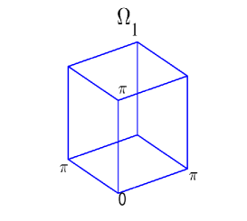
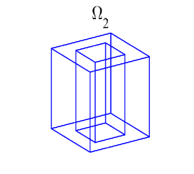
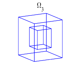
Figure 1: The three 3D domains. $\Omega_{1}$ is a cube $\left[0\;,\;\pi\right]^{3}$. $\Omega_{2}$ is the cube with a tunnel $\left[\frac{\pi}{4}\;,\;\frac{3\pi}{4}\right]^{2}\times\left[0\;,\;\pi\right]$. $\Omega_{3}$ is the cube with a void $\left[\frac{\pi}{4}\;,\;\frac{3\pi}{4}\right]^{3}$ inside.

The last two domains result in nontrivial $\mathbb{C}_{0}$ for the two constrained problems, respectively.

We use uniformly cubic mesh for all the problems. The mesh size is set to $h=\frac{\pi}{32}$ uniformly. We use the first order Nédélec to construct the matrix system of the discrete weak formulation (79). The matrix $\mathcal{U}$ is chosen as in [5]:

$$\begin{split}\mathcal{U}=\frac{5}{h^{3}}\mathcal{I},\end{split}$$

where $\mathcal{I}\in\mathbb{R}^{M\times M}$ is the identity matrix. We use the Preconditioned Conjugate Gradient method (PCG) to compute the linear systems and use the Locally Optimal Block Preconditioned Conjugate Gradient method (LOBPCG) to compute eigenvalue problem in the equivalent problems. The right hand side $\mathcal{F}$ is taken as random data. As the discussion in Section 6.2, the $\mathcal{G}$ is generated by $\mathcal{G}=\mathcal{B}^{T}u$ with a random $u\in\mathbb{C}^{N}$. We use the ILU(0) preconditioner to accelerate the algorithms. By Theorem 6.1, for the equation with the term $\mathcal{M}\mathcal{H}\mathcal{H}^{T}\mathcal{M}$, the ILU(0) factors are generated by the sparse matrix $\mathcal{A}+\mathcal{B}\mathcal{U}\mathcal{B}^{T}+\mathcal{M}$. We use the error (91) to measure the convergence of the last equation in the equivalent problems and use relative errors for the other equations and the eigenvalue problem. The stopping criterion for the last equation is set to $10^{-10}$. As the last equation depends on the solution of other equations, the stopping criteria for other equations and eigenvalue problems should be smaller than the last one. We set them to $10^{-11}$.

7.1 Example 1

The first numerical example is the mixed Maxwell problem with Dirichlet boundary condition on the domain $\Omega_{1}$:

$$\begin{split}\nabla\times\nabla\times\mathbf{u}+\nabla\mathbf{p}&=\mathbf{f}\quad\;\text{in}\;\quad\Omega_{1},\\ \nabla\times\mathbf{u}&=\mathbf{g}\quad\,\text{in}\;\quad\Omega_{1},\\ \mathbf{n}\times\mathbf{u}&=0\quad\,\text{on}\quad\partial\Omega_{1},\\ \mathbf{p}&=0\quad\,\text{on}\quad\partial\Omega_{1}.\\ \end{split}$$ (98)

In this problem, the matrix $\mathcal{B}$ are full-rank. We can use the direct method to solve the exact solution of its matrix system. We also use the direct method to solve the solution of the penalty method (97). Figure 2 shows the the relative error of the penalty solution $u_{\varepsilon}$ compared with the exact solution. The error of $u_{\varepsilon}$ goes down with the penalty parameter $\varepsilon$ becoming large at first. After some point, the error goes up with $\varepsilon$ continuing becoming large. The reason of this phenomenon is that the machine precision is limited and the parameter is too large.

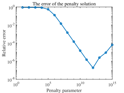
Figure 2: The relative error of the solution $u_{\varepsilon}$ of penalty method (97) for the discrete problem of (98) with the exact solution.

As $\dim\mathbb{C}_{0}=0$ and $c=0$ in this problem, we use the equivalent problems (69) and (74) to solve its matrix system, respectively. When using the equivalent problem (74), we use the simultaneous iteration for the two equations. The error is measured after each iteration. Figure 3 shows the convergence histories in solving the equivalent problems with PCG. The results illustrate that the ILU(0) preconditioner reduces the iteration counts.

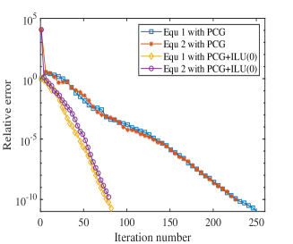
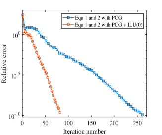
Figure 3: The convergence histories of the equivalent problem (69) (left) and (74) (right) in solving the discrete problems of the equation (98).

7.2 Example 2

The second example is also the mixed Maxwell equation on the domian $\Omega_{1}$ but with Neumann boundary condition:

$$\begin{split}\nabla\times\nabla\times\mathbf{u}+\nabla\mathbf{p}&=\mathbf{f}\quad\;\text{in}\;\quad\Omega_{1},\\ \nabla\times\mathbf{u}&=\mathbf{g}\quad\,\text{in}\;\quad\Omega_{1},\\ \mathbf{n}\times(\nabla\times\mathbf{u})&=0\quad\,\text{on}\quad\partial\Omega_{1},\\ \mathbf{n}\cdot\nabla\mathbf{p}&=0\,\quad\text{on}\quad\partial\Omega_{1}.\\ \end{split}$$ (99)

In this example, it is still that $\dim\mathbb{C}_{0}=0$ and $c=0$ as the first example. But the columns of $\mathcal{B}$ are no longer full-rank. This means that its matrix system is not invertible and the direct method is invalid for the problem. We use the equivalent problem (69) and (74) to solve this problem, respectively. Figure 4 shows the convergence histories of PCG method with and without ILU(0) preconditioner.

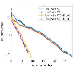
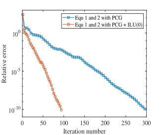
Figure 4: The convergence histories of the equivalent problem (69) (left) and (74) (right) in solving the discrete problems of the equation (99).

7.3 Example 3

The third numerical example is the mixed Maxwell equation with Neumann boundary condition on the domian $\Omega_{2}$:

$$\begin{split}\nabla\times\nabla\times\mathbf{u}+\mathbf{u}+\nabla\mathbf{p}&=\mathbf{f}\quad\;\text{in}\,\quad\Omega_{2},\\ \nabla\times\mathbf{u}&=\mathbf{g}\quad\,\text{in}\;\quad\Omega_{2},\\ \mathbf{n}\times(\nabla\times\mathbf{u})&=0\quad\,\text{on}\quad\partial\Omega_{2},\\ \mathbf{n}\cdot\nabla\mathbf{p}&=0\quad\,\text{on}\quad\partial\Omega_{2}.\\ \end{split}$$ (100)

Because there is a tunnel in this domain, the cohomology space of this form is not empty and $\dim\mathbb{C}_{0}=1$. We use the equivalent problem (67) to solve the matrix system of this problem. Figure 5 shows the convergence histories of the eigenvalue problem and linear systems

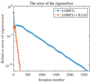
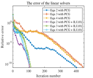
Figure 5: The convergence histories of the eigenvalue problem (left) and linear systems (right) of the equivalent problem (67) in solving the discrete problem of the equation (100).

7.4 Example 4

The fourth example is the constrained grad-div problem on the domain $\Omega_{1}$:

$$\begin{split}-\nabla(\nabla\cdot\mathbf{u})+\nabla\times\mathbf{p}&=\mathbf{f}\quad\;\text{in}\;\quad\Omega_{1},\\ \nabla\times\mathbf{u}&=\mathbf{g}\quad\,\text{in}\;\quad\Omega_{1},\\ \mathbf{n}(\nabla\cdot\mathbf{u})&=0\quad\,\text{on}\quad\partial\Omega_{1},\\ \mathbf{n}\times(\nabla\times\mathbf{p})&=0\quad\,\text{on}\quad\partial\Omega_{1}.\\ \end{split}$$ (101)

In this problem, $\dim\mathbb{C}_{0}=0$ and $c=0$. We use the equivalent problem (69) and (74) to solve this problem, respectively. Figure 6 shows the convergence histories of PCG method with and without ILU(0) preconditioner.

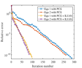
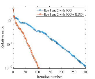
Figure 6: The convergence histories of the equivalent problem (69) (left) and (74) (right) in solving the discrete problems of the equation (101).

7.5 Example 5

The fifth numerical example is the constrained grad-div problem on the domain $\Omega_{3}$:

$$\begin{split}-\nabla(\nabla\cdot\mathbf{u})+\mathbf{u}+\nabla\times\mathbf{p}&=\mathbf{f}\quad\;\text{in}\;\quad\Omega_{3},\\ \nabla\times\mathbf{u}&=\mathbf{g}\quad\,\text{in}\;\quad\Omega_{3},\\ \mathbf{n}(\nabla\cdot\mathbf{u})&=0\quad\,\text{on}\quad\partial\Omega_{3},\\ \mathbf{n}\times(\nabla\times\mathbf{p})&=0\quad\,\text{on}\quad\partial\Omega_{3}.\\ \end{split}$$ (102)

Similar to the third example, the cohomology space of this form is also not empty and $\dim\mathbb{C}_{0}=1$ because of the void in this domain. We use the equivalent problem (67) to solve the matrix form of this problem. Figure 7 shows the convergence histories of the eigenvalue problem and linear systems.

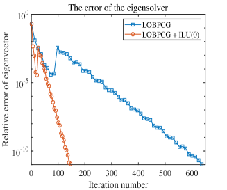
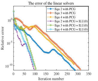
Figure 7: The convergence histories of the eigenvalue problem (left) and linear systems (right) of the equivalent problem (67) in solving the discrete problem of the equation (102).

8 Conclusions

In this paper, we consider solving the discrete systems of the constrained problems on de Rham complex. The first difficulty is the poor condition of the discrete systems. Many existing iterative methods and preconditioning techniques do not work for such systems. The second difficulty is that the systems are non-invertible in the case that the inf-sup condition about the constraint term is not satisfied, even if the desired component in the system is still unique.

We discretize the constrained problems use the finite element complex. We prove that the matrices in the algebraic system satisfy the property $\mathcal{A}\mathcal{M}^{-1}\mathcal{B}=0$. This property corresponds to the property $d^{2}=0$ on complex. This is an extra property of the systems in this paper compared with general constrained problems. By this property, we prove that the explicit Hodge decomposition of the right hand side can be obtained through solving a Hodge Laplacian. We construct several equivalent problems for the discrete systems. No mater whether inf-sup condition is satisfied or not, only if the component $\mathbf{u}_{h}$ is unique, we can solve it though some well-posed problems in the equivalent problems. Furthermore, the spectral distributions of the equations contained in these equivalent problems are Laplace-like, if the complex is Fredholm. Then many existing iterative methods and preconditioning techniques can be applied to solving them. In our paper [5], we have discussed how to solve the linear equations and eigenvalue problems in the equivalent problems. This make the large-scalar constrained discrete problem become easy to solve.

We provide several numerical experiments on $\mathbb{R}^{3}$ complex to verify the equivalent problems. The numerical results show the capability and efficiency of the methods that we propose.

References

- [1] Douglas N. Arnold. Finite element exterior calculus. SIAM, 2018.
- [2] Douglas N. Arnold, Richard S. Falk, and Ragnar Winther. Finite element exterior calculus, homological techniques, and applications. Acta Numerica, pages 1–155, 2006.
- [3] Douglas N. Arnold, Richard S. Falk, and Ragnar Winther. Finite element exterior calculus: from hodge theory to numerical stability. Bulletin of the American mathematical society, 47(2):281–354, 2010.
- [4] Daniele Boffi, Franco Brezzi, and Michel Fortin. Mixed Finite Element Methods and Applications, volume 44. Springer, 2013.
- [5] Zhongjie Lu. Auxiliary iterative schemes for the discrete operators on de Rham complex. https://arxiv.org/abs/2105.02065.
- [6] Kent-Andre Mardal and Ragnar Winther. Preconditioning discretizations of systems of partial differential equations. Numer. Linear Algebra Appl., 18(1):1–40, 2011.
- [7] Jean-Claude Nédélec. Mixed finite elements in . Numerische Mathematik, 35(3):315–341, 1980.