The Spacetime Picture in Quantum Gravity II

Abstract

As a continuation to [12], we introduce a new formalism for (part of) QG, which we call TQG, since it’s based on the NC Tori. This allows us to obtain numerous insights about the nature of time, like its discretization, its regular pace at the macroscopic scale, a solution to the Problem of Time, and a connection with the Measurement Problem and wave function collapse.

 

Introduction

 

In the phase space of Gravity, there’s no background spacetime (both in terms of manifold and metric), and this leads to a Hamiltonian $\mathcal{H}_{EH}=\sum_{i}N_{(i)}\mathbf{C}^{(i)}$ given by the constraints $\mathbf{C}^{(i)}$, which, in turn, leads to gauge invariant phase space properties (“Dirac properties”) $F$ (i.e., the ones that commute with the constraints, $\left\{F,\mathbf{C}^{(i)}\right\}=0$) that lack an adequate time evolution (since $\frac{\partial F}{\partial t}=\left\{F,\mathcal{H}_{EH}\right\}=$$\sum_{i}N_{(i)}\left\{F,\mathbf{C}^{(i)}\right\}=0$.) We claim that Dirac properties are not the relevant thing to look for. For example, one can show that the total volume of a solution $g$ is not a Dirac property, even when it’s a diffeomorphism invariant functional [2]. But the problem is not in the volume, it’s in the notion of Dirac property. Indeed, the reason for the previous seemingly paradoxical issue is directly related to the fact that the constraints in GR do not implement the full spacetime diffeomorphism group on phase space, and this is a consequence of the fact that the slicing of spacetime with spacelike Cauchy surfaces (which is needed to build the phase space) is dependent on the dynamical metric [2]. Thus, Dirac properties are phase space properties, and very tied to its structure. The issue about diffeomorphism invariant properties in a solution, but which are not Dirac properties, is, again, an artifact of the phase space picture, like the “no time” problem. To avoid all of these problems, we propose to completely dispense from the phase space picture when dealing with geometrical properties of spacetime, and instead switch to a spacetime picture. The only reason why we consider the Hamiltonian formulation (and, thus, the phase space picture and Dirac properties) is because it’s needed for the process of canonical quantization. But, once we canonically quantize a kinematical algebra, we can build the relational spacetime algebra and start to work in the spacetime picture and thus forget about the phase space; only if we are trapped in the phase space picture we would need to consider Dirac properties. When we work in basic GR in the spacetime picture and solve the field equations in simple cases, we don’t even think about Dirac properties, we just consider the diffeomorphism invariant properties of the solution in question, like the spacetime volume (and, of course, also the time evolution with respect to this solution; it doesn’t make sense to look for “time evolutions in the phase space of GR” since there’s no spacetime in it, it’s only when we pick a solution, a metric, that we can build the relational spacetime, as was argued here: time evolution is the specific change with respect to a duration, the variable with respect to which one measures the change must have that specific physical interpretation; thus, since we need anyway to pick a solution to build the relational spacetime and the time evolution, the need to build Dirac phase space properties in order to consider their “phase space time evolution” completely dissolves, since by definition we must abandon the phase space picture if we want to build a true time evolution; the imperative of Dirac properties in QG comes from the assumption that we need, and can, build a true time evolution in the phase space of GR, for which, naturally, one would need to consider the phase space version of diffeomorphism invariance, namely, Dirac properties, an a notion of relational time not related to duration, a property of the gravitational field, but to other fields, if that is even possible in the first place.)

 

Thus, the problem here will be assumed to be that of trying to find an analogue of duration with respect to a given metric (i.e., in a spacetime picture) but now in the quantum (gravity) realm.

 

Background

 

We review and summarize below some of the basic notions from [12] that will be relevant in the present paper, which is a continuation. We follow here the numeration for the definitions and propositions from that reference, where a more detailed discussion can be found.

 

$\mathbf{Definition\;1.1}$: The (kinematical) phase space of GR is defined as

$$X=\left\{\left[h_{ab},\pi^{ab}\right]\diagup h_{ab},\pi^{ab}\in C^{\infty}(\varSigma)\,(\mathrm{as\,fields}\,\mathrm{on}\,\varSigma)\right\},$$

where $h_{ab}$ and $\pi^{ab}$ are, respectively, a smooth riemannian metric on a spacelike Cauchy hypersurface $\Sigma$ in a compact and boundaryless spacetime $M$, foliated by $\Sigma$ as usual, and the conjugate momentum tensor density$.\,\blacksquare$

 

$\mathbf{Definition\;1.2}$: The subset $\mathcal{F}\subset C(X)$ consists of the phase space functionals of the form

$$F_{f}\left(\left[h_{ab},\pi^{ab}\right]\right)\doteq\int_{\varSigma}f\boldsymbol{\epsilon}(h_{ab}),\,\forall\left[h_{ab},\pi^{ab}\right]\in X,$$

where $f\in C^{\infty}(\varSigma)$ and $\boldsymbol{\epsilon}(h_{ab})$ is the volume element of $h_{ab}$, i.e. $\boldsymbol{\epsilon}(h_{ab})=\sqrt{h}\,\mathrm{d}^{3}x$ ($h=\mathrm{det}\,(h_{ab})$)$.\,\blacksquare$

 

$\mathbf{Proposition\;1.1}$: The assignment $f\,\longmapsto F_{f}$ is injective.$\,\square$

 

$\mathbf{Definition\;1.3}$: We now define a mapping $R:\mathcal{F}\times X\,\longrightarrow C^{\infty}(\varSigma)\times Obj(\mathsf{Hil})$ (where $Obj(\mathsf{Hil})$ is the collection of objects in the category $\mathsf{Hil}$ of Hilbert spaces) by

$$(F_{f},\left[h_{ab},\pi^{ab}\right])\,\longmapsto R(F_{f},\left[h_{ab},\pi^{ab}\right])\doteq(f,L^{2}(\mathcal{S},\boldsymbol{\epsilon}(h_{ab})),$$

(where $\mathcal{S}$ is the $C^{\infty}(\varSigma)-$module of smooth spinor fields in $\varSigma$, which from now on we assume allows a spin structure)$.\,\blacksquare$

 

$\mathbf{Definition\;1.4}$: For fixed $\left[h_{ab},\pi^{ab}\right]\in X$ and variable $F_{f}\in\mathcal{F}$, we denote the first component of $R(F_{f},\left[h_{ab},\pi^{ab}\right])$ as $R_{h}(F_{f}).\,\blacksquare$

 

$\mathbf{Definition\;1.5}$: We make $\mathcal{F}$ into an (unital) algebra $(\mathcal{F},$$\cdot_{sp.})$, where the product $\cdot_{sp.}$ in $\mathcal{F}$ is defined as

$$\left(F_{f_{1}}\cdot_{sp}F_{f_{2}}\right)\left(\left[h_{ab},\pi^{ab}\right]\right)\doteq F_{f_{1}f_{2}}\left(\left[h_{ab},\pi^{ab}\right]\right),\,\forall\left[h_{ab},\pi^{ab}\right]\in X$$

$$=\int_{\varSigma}f_{1}f_{2}\boldsymbol{\epsilon}(h_{ab}).\,\blacksquare$$

 

$\mathbf{Corollary\;1.1}$: The map $R_{h}$ is a bijection beetwen $\mathcal{F}$ and $C^{\infty}(\varSigma)$ (by Proposition 1.1), and is a faithfull algebra representation of $\mathcal{F}$ into $\mathcal{B}\left(L^{2}(\mathcal{S},\boldsymbol{\epsilon}(h_{ab}))\right)$ by multiplication operators, i.e. $R_{h}(F_{f})(\psi)(x)\doteq f(x)\psi(x),\,\forall\psi\in L^{2}(\mathcal{S},\boldsymbol{\epsilon}(h_{ab}))$$.\,\square$

 

We call $R_{h}$ the “relational representation”, since it gives a way of obtaining the algebra of physical $3-$space purely from Field properties (represented here by the phase space functionals). Switching to a relational and algebraic frame of mind, we can take this representation as the actual way of defining how to build space from the phase space algebra of the gravitational field.

 

$\mathbf{Proposition\;1.2}$: If one starts with a subset $\mathcal{A}_{\varSigma}$ (with a commutative product $\cdot_{sp}$) of the phase space algebra $\mathcal{A}_{X}$ (i.e. $\mathcal{A}_{\varSigma}\subset\mathcal{A}_{X}$, but only as a set and not as a subalgebra), which correspond, respectively, to $\mathcal{F}$ and $C(X)$ but seen as abstract algebras, then there exist a purely algebraic (i.e. which doesn’t make use of the commutative manifold structure of space for its definition) faithful representation $\left(\widetilde{R}_{h}\left[\mathcal{A}_{\varSigma}\right],\mathcal{H}_{\widetilde{R}_{h}}\right)$ of $\mathcal{A}_{\varSigma}$ and isomorphisms $\pi_{X}:\mathcal{A}_{\varSigma}\,\longrightarrow\mathcal{F}$ and $\pi_{\varSigma}:\widetilde{R}_{h}\left[\mathcal{A}_{\varSigma}\right]\,\longrightarrow C^{\infty}(\varSigma)$, such that the following diagram commutes:

i.e. such that

$$R_{h}=\pi_{\varSigma}\circ\widetilde{R}_{h}\circ\pi_{X}^{-1}.\,\square$$

 

Note that, in the general, non-commutative case, only the left hand side of the previous diagram survives. In this way, all the geometrical information of the space is now contained in the spectral triple.

 

$\mathbf{Definition\;2.1}$: Consider the phase space of GR, $(X,C(X),\left\{\cdot,\cdot\right\}_{GR})$, and a background independent Poisson sub-algebra $\mathcal{A}_{GR}$ of phase space functionals there. The basic ${}^{*}-$algebra, $\widehat{\mathcal{A}}_{QG}$, in QG will be the algebra $S_{\mathcal{A}_{GR}}$ freely generated (with field $\mathbb{C}$) by the classical algebra elements and with the relations imposed by the ideals $\mathcal{I}_{*LP}$ (where $*$ is the involution, $L$ is from linear and $P$ from $\mathrm{i}$ multiplied by the Poisson brackets. This process simply imposes the familiar Dirac commutation relations of canonical quantization to $\widehat{\mathcal{A}}_{QG}$, that is: $\left[\widehat{a},\widehat{a}^{\prime}\right]_{\widehat{\mathcal{A}}_{QG}}\doteq$$\widehat{a}\star_{\widehat{\mathcal{A}}_{QG}}\widehat{a}^{\prime}-\widehat{a}^{\prime}\star_{\widehat{\mathcal{A}}_{QG}}\widehat{a}=$$\mathrm{i}\widehat{\left\{a,a^{\prime}\right\}}_{GR}$, where $\star_{\widehat{\mathcal{A}}_{QG}}$ is the quantum probability algebraic product of $\widehat{\mathcal{A}}_{QG}$). That is, $\widehat{\mathcal{A}}_{QG}$ is the quotient:

$$\widehat{\mathcal{A}}_{QG}\doteq\frac{S_{\mathcal{A}_{GR}}}{\mathcal{I}_{*LP}}.\,\blacksquare$$

 

The next task is to identify a subalgebra $\widehat{\mathcal{A}}_{SP.}\subset\widehat{\mathcal{A}}_{QG}$ that plays a role equivalent to the one of $\mathcal{A}_{\varSigma}$ in the classical case of Proposition 1.2.

 

$\mathbf{Definition\;2.2}$: Consider the subset $\{f_{S}\}$ of all elements $f_{S}$ in $\mathcal{F}$ with $S\doteq supp\,f_{S}\subseteq\varSigma$, then we can see $\mathcal{F}$ as the result of the application of an indexation relation $\widetilde{I}_{\mathcal{F}}:I\,\longrightarrow\mathcal{F},\,S\,\longmapsto\widetilde{I}_{\mathcal{F}}(S)\doteq\{f_{S}\}$, where $I$ is the collection of all the supports $S$. We now replace $I$ by a subset $I_{Dis}\subset I$ which can be at most countably infinite, and compute the Poisson brackets in $\mathcal{F}_{Dis}\doteq\widetilde{I}_{\mathcal{F}}[I_{Dis}]$: the subset $I_{Dis}$ should be selected in a way that makes $(\mathcal{F}_{Dis},\left\{\cdot,\cdot\right\}_{GR})$ a Poisson subalgebra and, in particular, one whose structure constants don’t depend on the differentiable manifold details of $\Sigma$ nor on the details of the functions $f_{S}$ varying over it, but only on $I_{Dis}$, as an indexing set. With this set up, we choose $\mathcal{A}_{GR}$ such that $\mathcal{F}_{Dis}\subset\mathcal{A}_{GR}$ (so that $\widehat{\mathcal{F}}_{Dis}\subset\widehat{\mathcal{A}}_{QG}$) and define:

$$\widehat{\mathcal{A}}_{SP.}\doteq\widehat{\mathcal{F}}_{Dis}.\,\blacksquare$$

 

$\mathbf{Definition\;2.3}$: Assuming one has the family of possible representations $\left(R_{QG}\left[\widehat{\mathcal{A}}_{QG}\right],\mathcal{H}_{R_{QG}}\right)$ of $\widehat{\mathcal{A}}_{QG}$, we define as

$$\widehat{\mathcal{A}}_{sp.}\doteq R_{QG}\left[\widehat{\mathcal{A}}_{SP.}\right]$$

the non-commutative algebra of quantum physical $3-$space that “relationally arises” from the quantum gravitational field (this algebra will be the quantum analogue of $\widetilde{R}_{h}\left[\mathcal{A}_{\varSigma}\right]$, and $R_{QG}$ that of $\widetilde{R}_{h}$, in the left hand side of the diagram of Proposition 1.2)$.\,\blacksquare$

 

$\mathbf{Definition\;2.6}$: The analogue of a given classical metric $h_{ab}$ will be given by a $3-$(spectral) dimensional real first order spectral triple

$$\mathcal{T}_{D_{QG}}^{R_{QG}}\doteq\left(R_{QG}\left[\widehat{\mathcal{A}}_{SP\mathchar 46\relax}\right],\mathcal{H}_{R_{QG}},D_{QG}\right)\mathchar 46\relax\,\blacksquare$$

 

$\mathbf{Remark\;2.2}$: In particular, the Dirac-like operators $D_{QG}$ could be used to calculate non-commutative space intervals (i.e. distances) and non-commutative volume integrals, which, given the interpretations we made, are the genuinely quantum distances and volumes, since they are based on the quantized space algebra$\mathchar 46\relax\,\blacksquare$

 

2.3. TQG Relational Time

 

Regarding time, we have the following situation. If we recall the definition of the variables used in our relational construction of the space picture (Definition 1.2), the natural generalization needed to include time, and in this way to get a spacetime picture, would be

$$F_{f}\left(\left[h,\pi\right]\right)\doteq\int_{M}f(t,\overrightarrow{x})\,\sqrt{-g}\,\mathrm{d}^{4}x.$$

Thus, we can see that if we want to get time into the picture, we need to consider test functions $f$ whose support is spacetime rather than just space. Nevertheless, there are two problems with the previous generalization, namely: i) how do we get an identification $g_{ab}\,\longleftrightarrow\left[h,\pi\right]$ between smooth spacetime metrics $g_{ab}$ which are solutions and phase space points $\left[h_{ab},\pi^{ab}\right]$?; ii) even if we solve that, is the resulting assignment $f\,\longmapsto F_{f}$ injective? Regarding point i), it’s well known that the Gravitational Field Equations have a well-posed initial value formulation, that is, an initial value $\left[h_{ab},\pi^{ab}\right]\in X$ which satisfies the initial value constraints, and a gauge fixing of the lapse $N$ and shift $N^{a}$ in $\varSigma$ (this if we use the so called “wave gauge” [11, 1]) determines a unique smooth and globally hyperbolic solution $g_{ab}\,\underset{N,N^{a}}{\longleftrightarrow}\left[h_{ab},\pi^{ab}\right]$. For point ii), we have the following proposition.

 

$\mathbf{Proposition\;2.4}$: For spacetime functions $f$ with support in $[0,\epsilon)\times\varSigma$, the assignment $f\,\longmapsto F_{f}$ is injective in the limit $\epsilon\,\longrightarrow 0$.

 

Proof: from now on, we take, once and for all, $N=1$ and $N^{a}=0$ (both, in $\varSigma$): thus, we will work with the identification $g_{ab}\,\underset{1,0}{\longleftrightarrow}\left[h_{ab},\pi^{ab}\right]$. Now, at the infinitesimal level, the infinitesimal arc of the graph of a real variable function $h(t)\equiv\mathrm{det}\,(h_{ab})$ at some point (say, $t=0$) can be approximated by the tangent line at that point. To describe the latter, we need the value $h(0)$ and its derivative $\dot{h}(0)$. In the wave gauge, $\sqrt{-g}=N\sqrt{h}$ in $\varSigma$, i.e., at $t=0$, and, with our choice $N(0)=1$, we get $\sqrt{-g}(0)=\sqrt{h}(0).$ For $t\neq 0$,

$$g\equiv\mathrm{det}\,(g_{ab})=-g_{00}h+\sum_{i}g_{0i}d_{i},$$

where $d_{i}$ are the remaining determinants. In this way,

$$\dot{g}=-\dot{g}_{00}h-g_{00}\dot{h}+\sum_{i}\dot{g}_{0i}d_{i}+\sum_{i}g_{0i}\dot{d}_{i}.$$

But now, at $t=0,$ $g_{00}=-1$, $g_{0i}=0,$ and then $d_{i}=0$. Also, $\dot{h}=-2hK$ (where $K=-\frac{1}{2}h^{ab}\dot{h}_{ab}$; note that $\pi=2\sqrt{h}K$), while it can be determined from the wave gauge conditions that $\dot{g}_{00}=-K$ (recall that the wave gauge condition on the coordinates is

$$\sum_{\mu,\nu}g^{\mu\nu}\varGamma_{\mu\nu}^{\alpha}=0,\,\forall\alpha,$$

which means that the coordinates satisfy the wave equation; in our variables, at $t=0$, we get from it:

$$\dot{g}_{00}+Nh^{ab}K_{ab}=0.)$$

Thus, we get $\dot{g}(0)=-h(0)K(0)$. What all this means is that the tangent line to the graph of $\sqrt{-g}$ at $t=0$ only depends on $\left[h_{ab},\pi^{ab}\right]\in X$. Of course, due to the second order character of the Gravitational Field Equations, the initial data $\left[h_{ab},\pi^{ab}\right]\in X$ is arbitrary, which means that the tangent line can be arbitrary. Note that this is not trivial and we got it thanks to the wave gauge condition: if this condition implied, instead, that $\dot{g}_{00}=-2K$, then we would get $\dot{g}(0)=0$, which means that this derivative cannot be arbitrary, even if $\left[h_{ab},\pi^{ab}\right]\in X$ is. Of course, it’s actually this derivative the most important thing that we need here in order to probe beyond $\varSigma$ in the time direction$.\,\square$

 

$\mathbf{Example\;2.3}$: Let’s analyse first these type of spacetime variables in the case of standard QFT on a fixed curved spacetime ($M,g_{ab})$ [1, 5]. Consider the usual scalar field $\varphi$ with a linear wave equation

$$g_{ab}\nabla^{a}\nabla^{b}\varphi=0.$$

Since this equation has a well-posed initial value formulation, one can identify the phase space with the space $\mathrm{Sol}.$ of smooth solutions. Then, for a spacetime test function $f\in C_{0}^{\infty}(M)$, one defines the following variable on that phase space:

$$\underline{\varphi}(f)(\varphi)\doteq\int_{M}\varphi f\boldsymbol{\epsilon}(g).$$

The Poisson brackets for these variables are then given by

$$\left\{\underline{\varphi}(f),\underline{\varphi}(f^{\prime})\right\}=-\Omega(Ef,Ef^{\prime})$$

$$=-\int_{M}fEf^{\prime}\boldsymbol{\epsilon}(g)=\int_{M}f^{\prime}Ef\boldsymbol{\epsilon}(g),$$

where $\Omega$ is the symplectic form on $\mathrm{Sol}.$ and the linear map $E:C_{0}^{\infty}(M)\,\longrightarrow\mathrm{Sol}.,$$\,f\,\longmapsto Ef$ is the advanced minus the retarded solution of the wave equation with source $f\in C_{0}^{\infty}(M)$. Now, consider the case in which the supports of $f$ and $f^{\prime}$ are causally disconnected, i.e., if $f(x)f^{\prime}(y)\neq 0\,\Longrightarrow y\notin J^{+}(x)\bigcup J^{-}(x)$ (where $J^{+/-}$ are the causal future and past, respectively.) But we also have that:

$$\int_{M}f^{\prime}Ef\boldsymbol{\epsilon}(g)=\int_{\mathscr{R}_{1}}f^{\prime}(Af)\boldsymbol{\epsilon}(g)-\int_{\mathscr{R}_{2}}f^{\prime}(Rf)\boldsymbol{\epsilon}(g),$$

where $\mathscr{R}_{1}=supp\left(f^{\prime}\right)\bigcap J^{-}\left[supp\left(f\right)\right]$ and $\mathscr{R}_{2}=supp\left(f^{\prime}\right)\bigcap J^{+}\left[supp\left(f\right)\right]$, since $A(f)$ and $R(f)$ are, respectively, the advanced and retarded solutions. Thus, if the supports of $f$ and $f^{\prime}$ are causally disconnected, then, because of well-posedness of the field equation, clearly we have that $\mathscr{R}_{1}=\mathscr{R}_{2}=\textrm{\O}$ and in this way we get

$$\left\{\underline{\varphi}(f),\underline{\varphi}(f^{\prime})\right\}=-\Omega(Ef,Ef^{\prime})=0$$

for this case. On the other hand, if the supports are causally connected, we get

$$\left\{\underline{\varphi}(f),\underline{\varphi}(f^{\prime})\right\}=-\Omega(Ef,Ef^{\prime})\neq 0.\,\blacksquare$$

 

With the above in mind, let’s now go back to GR. In this theory, the field equations do not have the simple form of the previous linear wave equations, but comprise (in the so-called “wave gauge”), instead, what’s known as a quasi-linear system. For a scalar field with a quasi-linear field equation, the latter takes the form

$$g_{ab}(x;\varphi;\nabla^{c}\varphi)\nabla^{a}\nabla^{b}\varphi=F(x;\varphi;\nabla^{c}\varphi),$$

where $g_{ab}$ is a smooth lorentzian metric and $F$ a smooth function. These type of equations still have a well-posed initial value formulation, but they are quite different to the standard, ordinary wave equation. Indeed, the lorentzian metric that defines the character of the principal symbol of the differential operator now depends on the field variable. Of course, this makes the field equations non-linear. But, since the principal symbol of the operator is what determines how causal influences on this field propagate, it also means that the very causal structure is tied now to the variation of the field variable. Unfortunately, this fact makes all of the previous analysis of QFT in fixed curved spacetimes to be inapplicable here. Indeed, even to this date, the general form of the Poisson bracket for functionals like $F_{f}$ is not known [7]. Thus, a complete and rigorous quantization of time by following the recipe of our appraoch is definitely out of reach for now. Thus, it’s at this point when we start to make several approximations, which, we warn, may or may not be ultimately valid. We will judge that by the reasonability of their nature and of the results that follow from assuming them.

 

For simplicity, from now on we pretend a metric solution $g_{ab}$ is just a scalar field $\varphi$. These details will not matter here since the present analysis is only approximate and merely structural.

 

$\mathbf{Definition\;2.14}$: Consider a compact curve (timelike or spacelike) segment $\gamma$ in $M$. Then, on the phase space $X$ of GR, we define the following variables:

$$\underline{\varphi}(f_{\gamma})(\varphi)\doteq\int_{M}\varphi f_{\gamma}\boldsymbol{\epsilon}(\varphi),\,supp\,(f_{\gamma})=\gamma,\,f_{\gamma}\in C_{0}^{\infty}(M).\,\blacksquare$$

 

$\mathbf{Proposition\;2.5}$: The previous variables in Definition 2.14 can indeed be used to obtain $C^{\infty}(\gamma)$ via $R_{\varphi}$ (in the limit $\epsilon\,\longrightarrow 0$.)

 

Proof: as in Proposition 2.1 [12], we define the following product

$$(\underline{\varphi}(f_{\gamma}^{1})\cdot_{\gamma}\underline{\varphi}(f_{\gamma}^{2}))(\varphi)\doteq\underline{\varphi}(f_{\gamma}^{1}f_{\gamma}^{2})(\varphi),\,\forall\varphi\in X$$

$$=\int_{M}\varphi f_{\gamma}^{1}f_{\gamma}^{2}\boldsymbol{\epsilon}(\varphi).$$

In the limit $\epsilon\,\longrightarrow 0$, where the assignment $f_{\gamma}\,\longmapsto\underline{\varphi}(f_{\gamma})$ is injective (the term $\varphi$ in the integral can be handled by analogous arguments as those in Proposition 2.1), we get an algebra $\left\{\underline{\varphi}(f_{\gamma}k_{0})\right\}_{f_{\gamma}\in C_{0}^{\infty}(M);\cdot_{\gamma}}$, for each $k_{0}\in C^{\infty}(\gamma)$ ($k_{0}$ is non-zero for each point in $\gamma$; all algebras for different $k_{0}$ are isomorphic and equivalent to $C^{\infty}(\gamma)$), which, since the solution $\varphi$ such that $k_{0}=\varphi^{-1}$ is assumed to be non-vanishing on $\gamma$, is then bijectively mapped to $C^{\infty}(\gamma)$ via $R_{\varphi}(\underline{\varphi}(f_{\gamma}k_{0}))=f_{\gamma}$; but, since all the algebras are isomorphic, this means that the relational representation indeed induces the algebra $C^{\infty}(\gamma)$ of the curve $\gamma$ from a single algebra of phase space functions for any of those solutions $\varphi$$.\,\square$

 

Consider some subset of $\mathrm{Sol}.$ in which all metrics have conformally-equivalent causal structures (besides this requirement, there’s freedom for choosing any such subset.) Thus, while we have many different metrics, at least we have a single causal structure $\mathcal{C}$. Thus, the only variation we actually have now is that of the conformal factor among the different metrics. It’s this variation the one we will try to quantize. Nevertheless, the equations are still non-linear in that factor. For this, we will consider only the linear part for the quantization; that is, the result will be only kinematical, since the non-linear coupling is being ignored. In this way, what we are doing is to consider quantum spacetime geometries which are “benign” and “semi-classical” enough such that they have a defined causal structure and which remains more or less the same among the different geometries. Furthermore, they are also such that the conformal factor doesn’t vary non-linearly among them. Thus, the geometries are almost classical, the only variation is a “residual” one in the conformal factor, which is linear, and hyperbolic with respect to the causal structure $\mathcal{C}$. It’s only this variation that is quantized below.

 

$\mathbf{Definition\;2.15}$: A causal set (see, e.g., [8] and references therein) is a partially ordered set $\left(C,\leq_{\mathcal{C}}\right)$ such that:

• for all $x\in C,$ $x\leq_{\mathcal{C}}x$ (Reflexive);

• for all $x,y\in C,$ if $x\leq_{\mathcal{C}}y$ and $y\leq_{\mathcal{C}}x$, then $x=y$ (Antisymmetric);

• for all $x,y,z\in C$, if $x\leq_{\mathcal{C}}y$ and $y\leq_{\mathcal{C}}z$, then $x\leq_{\mathcal{C}}z$ (Transitive);

• for all $x,z\in C$, $\mid\left\{y\in C,\,x\leq_{\mathcal{C}}y\leq_{\mathcal{C}}z\right\}\mid<\aleph_{0}$ (Locally finite)$.\,\blacksquare$

 

$\mathbf{Definition\;2.16}$: Let $\leq_{\mathcal{C}}$ be the causal partial order on the points in $M$ induced by the causal structure $\mathcal{C}$. Now, consider a graph defined on all of the spacetime manifold $M$; furthermore, on each $\varSigma_{t}$, it gives one of the graphs considered earlier in the discussion of area, while the nodes of each of these graphs for different $\varSigma_{t}$ and $\varSigma_{t^{\prime}}$ are connected by timelike/causal (with respect to $\leq_{\mathcal{C}}$) edges (e.g., the previous curve $\gamma$ could be one of them), while the edges of the graphs in each $\varSigma_{t}$ are seen as spacelike separated (i.e., the nodes are not related by $\leq_{\mathcal{C}}$.) We denote each node as $P_{i}$, for a countable index $i$. Thus, the collection of elements (it’s more convenient to call them by this term rather than points)

$$C\doteq\left\{P_{i}\right\}_{i\in\mathbb{N}}^{\leq_{\mathcal{C}}}$$

forms a causal set. Consider the edges $\mathrm{e}_{P_{N_{1}}}$ and $\mathrm{e}_{P_{N_{2}}}$ such that $\mathrm{e}_{P_{N_{2}}}\subset J^{+}(\mathrm{e}_{P_{N_{1}}})$. We omit the endpoints and (semi) characterize $\mathrm{e}_{P_{*}}$ simply by its initial point $P_{*}$ (that is, $\mathrm{e}_{P_{*}}$ represents any of the edges with initial point $P_{*}$.) We take the variables $\underline{\varphi}(\chi_{\mathrm{e}_{P_{*}}})$ (for which $supp\left(\chi_{\mathrm{e}_{P_{*}}}\right)=\mathrm{e}_{P_{*}}$), where $\chi_{\mathrm{e}_{P_{*}}}$ is the characteristic function of the set $\mathrm{e}_{P_{*}}$, and the algebra $\mathcal{A}_{TQG}$ that they linearly generate (with real coefficients), and promote the labelings to elements $P_{*}$ from an abstract, countably infinite causal set $C$$.\,\blacksquare$

 

$\mathbf{Lemma\;2.6}$: The variables of the proof of Propostion 2.5, $\underline{\varphi}(f_{\gamma}k_{0})$ (considering the set of all the elements from all the algebras $\left\{\underline{\varphi}(f_{\gamma}k_{0})\right\}_{f_{\gamma}\in C_{0}^{\infty}(M);\cdot_{\gamma}}$ that were defined), subjected to the process of Definition 2.2, result in the variables of Definition 2.16 (the proof is identical to that of Lemma 2.3 [12])$\mathchar 46\relax\,\square$

 

Thus, in line with the principle of striping the continuum, this is equivalent to replacing $f_{\mathrm{e}_{P_{*}}}$ by $k\chi_{\mathrm{e}_{P_{*}}},$ where $\chi_{\mathrm{e}_{P_{*}}}$ is the characteristic function of the set $\mathrm{e}_{P_{*}}$ in $M$ and $k\in\mathbb{R}$. Note how this makes the limit $\epsilon\,\longrightarrow 0$ unnecessary since $\chi_{\mathrm{e}_{P_{*}}}$ doesn’t change its value along $t$, and then these type of functions on the finite segment $\mathrm{e}_{P_{*}}$ can be taken as the “true general functions on the infinitesimal curve segment $\mathrm{d}\mathrm{e}_{P_{*}}$.” Of course, $\chi_{\mathrm{e}_{P_{*}}}$ is not a smooth function, but this will not be relevant. That is, associated to $P_{*}$, we get a $1-$dimensional abstract vector space

$$\mathcal{A}_{P_{*}}\doteq\left\{k\underline{\varphi}(P_{*})\right\}_{k\in\mathbb{R}}\cong\mathbb{R}$$

generated by the sole element $\underline{\varphi}(P_{*})$. Now, of course, if we quantize this we get just a commutative algebra, since $\left\{\underline{\varphi}(f),\underline{\varphi}(f)\right\}=-\Omega(Ef,Ef)=0$ (because $\Omega$ is a symplectic form.)

 

Nevertheless, we cannot consider $\mathcal{A}_{P_{*}}$ alone, because

$$\mathrm{e}_{P_{N_{2}}}\bigcap J^{+}(\mathrm{e}_{P_{N_{1}}})\neq\textrm{\O}\;\mathrm{and}\;\left\{\underline{\varphi}(f_{\mathrm{e}_{P_{N_{1}}}}),\underline{\varphi}(f_{\mathrm{e}_{P_{N_{2}}}})\right\}=-\Omega(Ef_{\mathrm{e}_{P_{N_{1}}}},Ef_{\mathrm{e}_{P_{N_{2}}}})\neq 0.$$

But now, by the linearity of both $\Omega$ and $E$, and remembering that we replace $f_{\mathrm{e}_{P_{*}}}$ by $k\chi_{\mathrm{e}_{P_{*}}}$, and that $\mathcal{A}_{P_{*}}\cong\mathbb{\mathbb{R}}$, then it’s clear that, when passing to the abstract labelings, the symplectic form $\Omega$ becomes simply a symplectic form $\widetilde{\Omega}$ on the $2-$dimensional space $\mathbb{\mathbb{R}}^{2}$ and characterized by a simple $2\times 2$ skew matrix of the form

$$\left(\begin{array}[]{cc}0&\theta(P_{N_{1}},P_{N_{2}})\\ -\theta(P_{N_{1}},P_{N_{2}})&0\end{array}\right),$$

where

$$\theta(P_{N_{1}},P_{N_{2}})\doteq\Omega(E\chi_{\mathrm{e}_{P_{N_{1}}}},E\chi_{\mathrm{e}_{P_{N_{2}}}}),$$

thing which greatly simplifies the problem at the mathematical level.

 

$\mathbf{Definition\;2.17}$: We define: $\mathcal{F}_{Dis\mathchar 46\relax}\equiv\mathcal{A}_{ST\mathchar 46\relax}\equiv\mathcal{A}_{P_{N_{1}}P_{N_{2}}}\subset\mathcal{A}_{TQG}$, generated by the $\underline{\varphi}(f_{\mathrm{e}_{P_{N_{1}}}}),$ $\underline{\varphi}(f_{\mathrm{e}_{P_{N_{2}}}})$. Now, following Definition 2.2, the quantum algebra $\widehat{\mathcal{A}}_{ST\mathchar 46\relax}\equiv\mathcal{\widehat{A}}_{P_{N_{1}}P_{N_{2}}}$ will be the exponentiated (recall that the passing from the Heisenberg to the Weyl algebra is mandatory for quantization in QFT [1]) quantum algebra for the two quantized edges $\widehat{\mathrm{e}}_{P_{N_{1}}}$ and $\widehat{\mathrm{e}}_{P_{N_{2}}}$, and generated, then, by two abstract elements, $u_{1}$ and $u_{2}$, which satisfy the relation

$$u_{1}u_{2}=e^{2\pi i\theta(P_{N_{1}},P_{N_{2}})}u_{2}u_{1}.\,\blacksquare$$

 

$\mathbf{Example\;2.4}$: This algebra is well known in NCG [3], and is called the NC $2-$Torus, $\mathbb{T}_{\theta}^{2}$, with deformation parameter $\theta$, since it corresponds to the deformation of the algebra of the classical Torus $\mathbb{T}^{2}$ (defined as the set $\left[0,1\right]^{2}$ with opposite sides of the square identified, or as $\mathbb{T}^{1}\times\mathbb{T}^{1}$, where $\mathbb{T}^{1}$ is the unit circle.) More precisely, we consider the universal $C^{*}-$algebra $A_{\theta(P_{N_{1}},P_{N_{2}})}$ defined by these generators. For $(r_{1},r_{2})=r\in\mathbb{Z}^{2}$, define the polynomials $u^{r}\doteq e^{\pi ir_{1}r_{2}\theta(P_{N_{1}},P_{N_{2}})}u_{1}^{r_{1}}u_{2}^{r_{2}}$, then $A_{\theta(P_{N_{1}},P_{N_{2}})}\ni a=\sum_{r\in\mathbb{Z}^{2}}a_{r}u^{r}$, where $a_{r}\in\mathbb{C}$ and the sum converges in the $C^{*}$ norm $\parallel\cdot\parallel_{C^{*}}$. The NC $2-$Torus is the dense, smooth $*-$subalgebra, pre$C^{*}-$algebra $C^{\infty}(\mathbb{T}_{\theta}^{2})=\mathcal{\widehat{A}}_{\theta(P_{N_{1}},P_{N_{2}})}$ of $A_{\theta(P_{N_{1}},P_{N_{2}})}$, that is, $r\,\longmapsto a_{r}$ is of rapid decay (the $C^{*}-$algebra $A_{\theta(P_{N_{1}},P_{N_{2}})}$, of course, gives the algebra of continuous NC-“functions”.) Now, $\mathbb{T}^{2}$ forms a Lie group, and we can define an action of this group on $A_{\theta(P_{N_{1}},P_{N_{2}})}$ by setting, for any $z\in\mathbb{T}^{2}$,

$$z\cdot u^{r}\doteq z_{1}^{r_{1}}z_{2}^{r_{2}}u^{r}.$$

This action is generated by the following two, commuting derivations:

$$\delta_{j}(a)\doteq\left[\frac{\mathrm{d}}{\mathrm{d}t}e^{2\pi i\phi_{j}}\cdot a\right]\mid_{t=0},\,j=1,2,$$

where $e^{2\pi i\phi_{j}}$ belongs to the circle group $\mathbb{T}^{1}$ (i.e., complex numbers of norm equal to $1$.) The following trace defines a faithfull algebraic state on $A_{\theta(P_{N_{1}},P_{N_{2}})}$:

$$\omega(a)\doteq a_{0}.$$

Note that

$$\omega(a^{*}a)=\sum_{r\in\mathbb{Z}^{2}}\mid a_{r}\mid^{2}\leq\parallel a\parallel_{C^{*}}^{2}.$$

With it, we can form the GNS representation $\pi_{\omega}$ [5] of the algebra (that is, $\left(a,b\right)_{\mathcal{H}_{\omega}}\doteq\omega(a^{*}b)=\left(a^{*}b\right)_{0}=\sum_{r\in\mathbb{Z}^{2}}a_{r}^{*}b_{r}$.) We denote as $\underline{a}$ to the algebra elements when seen as elements in the Hilbert space $\mathcal{H}_{\omega}$ of the representation (whose cyclic vector is $\underline{I}$ and is irreducible) and the same for the derivations when seen as acting on the algebra representation. We can now define a Dirac operator by setting (on the dense domain $\underline{\mathcal{\widehat{A}}}_{\theta(P_{N_{1}},P_{N_{2}})}$)

$$D_{P_{N_{1}}P_{N_{2}}}\doteq-i\mathrm{a}(P_{N_{1}},P_{N_{2}})^{-\frac{1}{2}}\left[\sigma_{1}\underline{\delta}_{1}+\sigma_{2}\underline{\delta}_{2}\right],$$

where $\sigma_{1},\sigma_{2}$ are the first two Pauli matrices. In this way, one can see that

$$\left(\pi_{\omega}\left[A_{\theta(P_{N_{1}},P_{N_{2}})}\right],\mathcal{H}_{\omega},D_{P_{N_{1}}P_{N_{2}}}\right)$$

forms a $2-$dimensional spectral triple (the eigenbasis of $D_{P_{N_{1}}P_{N_{2}}}^{2}$ is given by $\left\{\underline{u}^{r}\right\}_{r\in\mathbb{Z}^{2}}$ tensored with the canonical basis of $\mathbb{C}^{2}$, with eigenvalues $\lambda_{r}=\mathrm{a}(P_{N_{1}},P_{N_{2}})^{-1}4\pi^{2}r\cdot r$ of multiplicity $M_{r}=2$.) Furthermore (after some adequate normalization),

$$\mathrm{area}_{D_{P_{N_{1}}P_{N_{2}}}}(\widehat{\mathcal{R}}_{N_{1}N_{2}})\doteq\mathrm{tr}^{+}(\mid D_{P_{N_{1}}P_{N_{2}}}\mid^{-2})$$

$$=\mathrm{a}(P_{N_{1}},P_{N_{2}}).$$

See [3] for more details$.\,\blacksquare$

 

$\mathbf{Remark\;2.10}$: Note that this doesn’t mean that the geometry of spacetime at the quantum level is simply a NC Torus, since the physical interpretation of the algebra elements that we made before doesn’t lead to this. Indeed, for $\theta=0$, $u_{1}$ and $u_{2}$ generate a classical, continuum Torus, while the $\underline{\varphi}(\chi_{\mathrm{e}_{P_{N_{1}}}})$ and $\underline{\varphi}(\chi_{\mathrm{e}_{P_{N_{2}}}})$ generate what’s left of the algebra of the edges after we eliminated the continuum. Thus, the Torus geometrical interpretation from NCG will not be relevant here, and we are just using/borrowing its algebra for our own purposes and particular interpretations$.\,\blacksquare$

 

$\mathbf{Remark\;2.11}$: The physical interpretation of $\mathrm{area}_{D_{P_{N_{1}}P_{N_{2}}}}(\widehat{\mathcal{R}}_{N_{1}N_{2}})$ when $P_{N_{2}}$ is the endpoint of $\mathrm{e}_{P_{N_{1}}}$ is as the quantized riemannian area of the coordinate surface $\mathcal{R}_{N_{1}N_{2}}$ of $\mathrm{e}_{P_{N_{1}}}\times\mathrm{e}_{P_{N_{2}}}$ in coordinate space (that is, we parallelly propagate $\mathrm{e}_{P_{N_{1}}}$ along $\mathrm{e}_{P_{N_{2}}}$, then set $P_{N_{2}}$ as having coordinates $(x_{1},x_{2})=(1,0)$ and the endpoint of $\mathrm{e}_{P_{N_{2}}}$ as $(1,1)$, and then map the whole surface to a rectangle $\mathcal{R}_{N_{1}N_{2}}$ in coordinate space). Of course, we lose the lorentzian character, but this is not a problem since that is already being taken into account by the causal structure $\mathcal{C}$, but this riemannian metric still gives information about the duration and lenght of the finite $2-$dimensional process described by the spacetime surface $\mathrm{e}_{P_{N_{1}}}\times\mathrm{e}_{P_{N_{2}}}$, that is, a process which happens to the whole edge $\mathrm{e}_{P_{N_{2}}}$ for the duration of $\mathrm{e}_{P_{N_{1}}}$. In this way, given that, in order to take into account the causal relation between the two edges, we need to consider the combined quantized algebras of each one (which in turns gives a noncommutative algebra due to the causal relation) and that the nontrivial Dirac operator on it forms a triple of dimension $2$, then this leads us to take the (somewhat expected) view in which

 

spacetime events at a quantum level (which we denote as $\mathsf{e}_{N_{1}N_{2}}$, for the one corresponding to $P_{N_{1}},P_{N_{2}}$) are given by $2-$dimensional processes, i.e., processes that happen to a thing of finite length in a finite amount of proper time; furthermore, for a given quantum spacetime (in the sense defined here), the passing from one event to another is evidently discretized since the graph is countably infinite$.\,\blacksquare$

 

$\mathbf{Lemma\;2.7}$: There exists a state $\underline{\psi}_{N_{1}N_{2}}\in\mathcal{H}_{\omega}$ such that

$$\left(\underline{\psi}_{N_{1}N_{2}},D_{P_{N_{1}}P_{N_{2}}}^{2}\underline{\psi}_{N_{1}N_{2}}\right)_{\mathcal{H}_{\omega}}=\mathrm{a}(P_{N_{1}},P_{N_{2}})^{-1}=\mathrm{area}_{D_{P_{N_{1}}P_{N_{2}}}}(\widehat{\mathcal{R}}_{N_{1}N_{2}})^{-1}.$$

 

Proof: since the triple is $2-$dimensional, then $\sum_{k=1}^{N}M_{k}\lambda_{k}(\mid D_{P_{N_{1}}P_{N_{2}}}\mid^{-2})$ must diverge as $\sum_{k=1}^{N}\frac{1}{k}\sim\mathrm{ln}\,N$ when $N\,\longrightarrow\infty$. This is similar to the inverse of the harmonic oscillator Hamiltonian in standard QM, for which

$$\psi_{s}(x)\doteq\pi^{-\frac{1}{4}}e^{-(x-s)^{2}/2},\,s\in\mathbb{R},$$

is a coherent/Gaussian state. This state can be written in terms of the eigenbasis $\left\{\varphi_{k}\right\}_{k\in\mathbb{N}\bigcup\left\{0\right\}}$ of the Hamiltonian as

$$\psi_{s}(x)=e^{-s^{2}/2}\sum_{k=0}^{\infty}\sqrt{\frac{\left(s^{2}/2\right)^{k}}{k!}}\varphi_{k}(x).$$

This suggests to define the following state in $\mathcal{H}_{\omega}$:

$$\underline{\psi}_{s}\doteq\frac{\left(e^{s^{2}/4}-1\right)^{-1}}{2}\sum_{\underset{r_{1}\neq 0;r_{2}\neq 0}{r\in\mathbb{Z}^{2}}}\sqrt{\frac{\left(s^{2}/4\right)^{\mid r_{1}\mid}}{\mid r_{1}\mid!}}\sqrt{\frac{\left(s^{2}/4\right)^{\mid r_{2}\mid}}{\mid r_{2}\mid!}}\underline{u}^{r}.$$

First we need to check if this series defines a state in the first place. Indeed:

$$\parallel\underline{\psi}_{s}\parallel_{\mathcal{H}_{\omega}}^{2}=\frac{\left(e^{s^{2}/4}-1\right)^{-2}}{4}\sum_{\underset{r_{1}\neq 0;r_{2}\neq 0}{r\in\mathbb{Z}^{2}}}\frac{\left(s^{2}/4\right)^{\mid r_{1}\mid}}{\mid r_{1}\mid!}\frac{\left(s^{2}/4\right)^{\mid r_{2}\mid}}{\mid r_{2}\mid!}$$

$$=1,\,\forall s\in\mathbb{R}.$$

Furthermore,

$$\left(\underline{\psi}_{s},D_{P_{N_{1}}P_{N_{2}}}^{2}\underline{\psi}_{s}\right)_{\mathcal{H}_{\omega}}=\mathrm{a}(P_{N_{1}},P_{N_{2}})^{-1}8\pi^{2}\frac{\left(e^{s^{2}/4}-1\right)^{-2}}{4}\times$$

$$\sum_{\underset{r_{1}\neq 0;r_{2}\neq 0}{r\in\mathbb{Z}^{2}}}\frac{\left(s^{2}/4\right)^{\mid r_{1}\mid}}{\mid r_{1}\mid!}\frac{\left(s^{2}/4\right)^{\mid r_{2}\mid}}{\mid r_{2}\mid!}(r_{1}^{2}+r_{2}^{2});$$

noting that

$$r_{*}^{2}s^{2\mid r_{*}\mid}=\frac{s^{2}}{4}\frac{\mathrm{d}^{2}}{\mathrm{d}s^{2}}s^{2\mid r_{*}\mid},$$

then

$$\sum_{\underset{r_{1}\neq 0;r_{2}\neq 0}{r\in\mathbb{Z}^{2}}}\frac{\left(s^{2}/4\right)^{\mid r_{1}\mid}}{\mid r_{1}\mid!}\frac{\left(s^{2}/4\right)^{\mid r_{2}\mid}}{\mid r_{2}\mid!}(r_{1}^{2}+r_{2}^{2})$$

$$=\frac{s^{2}}{2}\sum_{\underset{r_{1}\neq 0;r_{2}\neq 0}{r\in\mathbb{Z}^{2}}}\left(\frac{\mathrm{d}^{2}}{\mathrm{d}s^{2}}\frac{\left(s^{2}/4\right)^{\mid r_{1}\mid}}{\mid r_{1}\mid!}\right)\left(\frac{\left(s^{2}/4\right)^{\mid r_{2}\mid}}{\mid r_{2}\mid!}\right)$$

$$=e^{s^{2}/4}s^{2}\left(\frac{s^{2}}{2}+1\right)\left(e^{s^{2}/4}-1\right);$$

in this way:

$$\left(\underline{\psi}_{s},D_{P_{N_{1}}P_{N_{2}}}^{2}\underline{\psi}_{s}\right)_{\mathcal{H}_{\omega}}=\mathrm{a}(P_{N_{1}},P_{N_{2}})^{-1}\pi^{2}\frac{\left(e^{s^{2}/4}-1\right)^{-1}}{2}\times$$

$$e^{s^{2}/4}s^{2}\left(\frac{s^{2}}{2}+1\right).$$

Now, consider the following equation:

$$\pi^{2}\frac{\left(e^{s^{2}/4}-1\right)^{-1}}{2}e^{s^{2}/4}s^{2}\left(\frac{s^{2}}{2}+1\right)=1.$$

It has a single solution, given by the unique limit $s\longrightarrow 0$. We denote $\underline{\psi}_{s\longrightarrow 0}$ as $\underline{\psi}_{N_{1}N_{2}}$. Thus:

$$\left(\underline{\psi}_{N_{1}N_{2}},D_{P_{N_{1}}P_{N_{2}}}^{2}\underline{\psi}_{N_{1}N_{2}}\right)_{\mathcal{H}_{\omega}}=\mathrm{a}(P_{N_{1}},P_{N_{2}})^{-1}=\mathrm{area}_{D_{P_{N_{1}}P_{N_{2}}}}(\widehat{\mathcal{R}}_{N_{1}N_{2}})^{-1}.\,\square$$

 

$\mathbf{Remark\;2.12}$: In this way, at least formally, we can see $\underline{\psi}_{N_{1}N_{2}}$ as a “pure algebraic state” $\omega_{\underline{\psi}_{N_{1}N_{2}}}$ which acts as

$$\omega_{\underline{\psi}_{N_{1}N_{2}}}(D_{P_{N_{1}}P_{N_{2}}}^{2})\doteq\left(\underline{\psi}_{N_{1}N_{2}},D_{P_{N_{1}}P_{N_{2}}}^{2}\underline{\psi}_{N_{1}N_{2}}\right)_{\mathcal{H}_{\omega}}.$$

Therefore, we can set:

$$\mathcal{F}_{D_{P_{N_{1}}P_{N_{2}}}^{2}}(\omega_{\underline{\psi}_{N_{1}N_{2}}})\doteq\omega_{\underline{\psi}_{N_{1}N_{2}}}(D_{P_{N_{1}}P_{N_{2}}}^{2})=\mathrm{area}_{D_{P_{N_{1}}P_{N_{2}}}}(\widehat{\mathcal{R}}_{N_{1}N_{2}})^{-1}.$$

We can interpret this in the sense that $\mathcal{F}_{D_{P_{N_{1}}P_{N_{2}}}^{2}}$ represents the inverse area “function” and that there’s just a single point $\omega_{\underline{\psi}_{N_{1}N_{2}}}$ in which its value is defined. After we introduce more events (and when they commute with each other), we can lift the different $\mathcal{F}_{D_{P_{N_{1}}P_{N_{2}}}^{2}}$ into a function $\mathcal{F}_{\mathrm{area}_{N_{1}N_{2}}}$ “on” the algebra of all the considered points and which can be interpreted as the analogue of a “characteristic function” for the spacetime “point” $\omega_{\underline{\psi}_{N_{1}N_{2}}}$ (although, the value of the function is $\mathrm{area}_{D_{P_{N_{1}}P_{N_{2}}}}(\widehat{\mathcal{R}}_{N_{1}N_{2}})^{-1}$ rather than just $1$, that is, the event $\mathsf{e}_{N_{1}N_{2}}$ is marked or given a physical interpretation in a relational manner by a property of the quantum Gravitational Field.) In the classical case, its analogue would be $\phi_{j}(P)\chi_{\left\{P\right\}}:M\,\longrightarrow\mathbb{R}$, where $\phi_{j}(P)\chi_{\left\{P\right\}}(x)=0$ if $M\ni x\neq P$, $\phi_{j}(P)\chi_{\left\{P\right\}}(x)=\phi_{j}(P)$ if $x=P$, and $\phi_{j}(P)$ are coordinates based on properties of the field (like distances and proper times)$.\,\blacksquare$

 

The next step now is to add more events. To this end, consider the previous event $\mathsf{e}_{N_{1}N_{2}}$, a fd timelike edge $\overline{\mathrm{e}}_{P_{N_{2}}}$ whose initial point is $P_{N_{2}}$ (recall that $P_{N_{2}}$ is also the initial point of $\mathrm{e}_{P_{N_{2}}}$, but this edge is spacelike), and the event $\mathsf{e}_{\overline{N}_{2}N_{3}}$ generated by $\overline{\mathrm{e}}_{P_{N_{2}}}$ and the spacelike edge $\mathrm{e}_{P_{N_{3}}}$, where $P_{N_{3}}$ is the endpoint of $\overline{\mathrm{e}}_{P_{N_{2}}}$ (for notational consistency, from now on we will denote the previous timelike edge $\mathrm{e}_{P_{N_{1}}}$ as $\overline{\mathrm{e}}_{P_{N_{1}}}$, and the event $\mathsf{e}_{N_{1}N_{2}}$ as $\mathsf{e}_{\overline{N}_{1}N_{2}}$, even when we are not considering any spacelike edge from $P_{N_{1}}$.)

 

$\mathbf{Definition\;2.18}$: For two events, we have $4$ generators, namely, $u_{1}$, corresponding to $\overline{\mathrm{e}}_{P_{N_{1}}}$, $u_{2}$, to $\mathrm{e}_{P_{N_{2}}}$, $u_{3}$, to $\overline{\mathrm{e}}_{P_{N_{2}}}$, and $u_{4}$, to $\mathrm{e}_{P_{N_{3}}}$. In this way, the commutation relations are given by

$$u_{1}u_{2}=e^{2\pi i\theta(\overline{P}_{N_{1}},P_{N_{2}})}u_{2}u_{1},$$

$$u_{3}u_{4}=e^{2\pi i\theta(\overline{P}_{N_{2}},P_{N_{3}})}u_{4}u_{3},$$

$$u_{1}u_{3}=e^{2\pi i\theta(\overline{P}_{N_{1}},\overline{P}_{N_{2}})}u_{3}u_{1},$$

$$...\,etc.$$

We can recognize the first two as the algebras $\mathcal{\widehat{A}}_{\mathsf{e}_{\overline{N}_{1}N_{2}}}$, $\mathcal{\widehat{A}}_{\mathsf{e}_{\overline{N}_{2}N_{3}}}$, corresponding, respectively, to the events $\mathsf{e}_{\overline{N}_{1}N_{2}}$, $\mathsf{e}_{\overline{N}_{2}N_{3}}$; we denote the one generated by the third relation as $\mathcal{\widehat{A}}_{\overline{P}_{N_{1}}\overline{P}_{N_{2}}}$$.\,\blacksquare$

 

$\mathbf{Example\;2.5}$: These four generators form what is actually known as the NC $4-$Torus [3], that is, the smooth subalgebra $C^{\infty}(\mathbb{T}_{\Theta}^{4})$ of the universal $C^{*}-$algebra $A_{\Theta}$ defined by

$$A_{\Theta}\ni a\doteq\sum_{r\in\mathbb{Z}^{4}}a_{r}u^{r},$$

$$u^{r}\doteq e^{\pi i\sum_{\underset{j<k}{j,k=1}}^{4}r_{j}\Theta_{jk}r_{k}}u_{1}^{r_{1}}u_{2}^{r_{2}}u_{3}^{r_{3}}u_{4}^{r_{4}},$$

$$\Theta\doteq\left(\begin{array}[]{cccc}0&\theta(\overline{P}_{N_{1}},P_{N_{2}})&\theta(\overline{P}_{N_{1}},\overline{P}_{N_{2}})&\theta(\overline{P}_{N_{1}},P_{N_{3}})\\ -\theta(\overline{P}_{N_{1}},P_{N_{2}})&0&\theta(P_{N_{2}},\overline{P}_{N_{2}})&\theta(P_{N_{2}},P_{N_{3}})\\ -\theta(\overline{P}_{N_{1}},\overline{P}_{N_{2}})&-\theta(P_{N_{2}},\overline{P}_{N_{2}})&0&\theta(\overline{P}_{N_{2}},P_{N_{3}})\\ -\theta(\overline{P}_{N_{1}},P_{N_{3}})&-\theta(P_{N_{2}},P_{N_{3}})&-\theta(\overline{P}_{N_{2}},P_{N_{3}})&0\end{array}\right).$$

Of course, the subalgebra of elements $a$ such that $a_{(r_{1},r_{2},r_{3},r_{4})}=0$, for all $r_{3}\neq 0$, $r_{4}\neq 0$, is isomorphic to $\mathcal{\widehat{A}}_{\mathsf{e}_{\overline{N}_{1}N_{2}}}$, etc. Again, one can define the action of $z\in\mathbb{T}^{4}$ as

$$z\cdot u^{r}\doteq z_{1}^{r_{1}}z_{2}^{r_{2}}z_{3}^{r_{3}}z_{4}^{r_{4}}u^{r},$$

and the associated derivations

$$\delta_{j}(a)\doteq\left[\frac{\mathrm{d}}{\mathrm{d}t}e^{2\pi i\phi_{j}}\cdot a\right]\mid_{t=0},\,j=1,2,3,4;$$

also the algebraic state

$$\omega(a)\doteq a_{0},$$

its GNS representation, and, finally, the Dirac operator there:

$$D_{\varTheta}\doteq-i\left[\gamma_{1}\underline{\delta}_{1}+\gamma_{2}\underline{\delta}_{2}+\gamma_{3}\underline{\delta}_{3}+\gamma_{4}\underline{\delta}_{4}\right].$$

The generalization of all this to a finite number $n\in\mathbb{N}$ of events should be obvious by now. Of course, the algebra will be given by a NC $2n-$Torus$.\,\blacksquare$

 

$\mathbf{Remark\;2.13}$: Note that this NC $2n-$Torus doesn’t represent quantum spacetime (to start, it would be $2n-$dimensional!), what it actually represents is quantum phase space. The reason for this is that the relational representation only works for infinitesimal (in time) events at the classical level, while the time separation between two timelike edges fails to be of this type. Thus, the situation is the following: the full NC $2n-$Torus quantum algebra is the algebra of phase space, and, if we restrict to the sub-algebras corresponding to the NC $2-$Tori that define our individual quantum events, then we can now apply the relational representration on each of them and obtain a piece of quantum spacetime there. Furthermore, since now the Field portion that defines the events is finite, then these events can be seen as states in the quantum phase space too (more precisely, the spacetime support, represented by vectors like $\underline{\psi}_{N_{1}N_{2}}$, of these states, which, in combination with a Dirac operator, do give the state), unlike the classical case and the infinitesimal portions there. Nevertheless, the collection of all these geometries doesn’t form something that represents a metric on “the union of these regions” (in particular, the previous $D_{\varTheta}$ cannot be interpreted as this desired metric.) Note that if we change the value of the area of event $\mathsf{e}_{\overline{N}_{2}N_{3}}$, i.e., changing $D_{P_{N_{2}}P_{N_{3}}},$ then it must be considered to be a different event/state and its spectral triple direct summed (at the unexponentiated level) with the one of the previous value in order to have a phase space describing both$.\,\blacksquare$

 

We go back now to the parameter $\theta(\overline{P}_{N_{1}},P_{N_{2}})$. We flat in space the spacetime cylinders to spacetime sheets in the $xt$ spacetime plane and then, after integration of delta functions on the remaining two spatial variables, we have:

$$\theta(\overline{P}_{N_{1}},P_{N_{2}})=\int_{\mathrm{e}_{P_{N_{2}}}\bigcap J(\overline{\mathrm{e}}_{P_{N_{1}}})_{xt}}\chi_{\mathrm{e}_{P_{N_{2}}}}(x,t)(E\chi_{\overline{\mathrm{e}}_{P_{N_{1}}}})(x,t)\,\sqrt{-g}\mathrm{d}x\mathrm{d}t;$$

now, since $\mathrm{e}_{P_{N_{2}}}\bigcap J^{-}(\overline{\mathrm{e}}_{P_{N_{1}}})_{xt}=\emptyset$, then

$$\theta(\overline{P}_{N_{1}},P_{N_{2}})=\int_{\mathrm{e}_{P_{N_{2}}}\bigcap J^{+}(\overline{\mathrm{e}}_{P_{N_{1}}})_{xt}}\chi_{\mathrm{e}_{P_{N_{2}}}}(x,t)(R\chi_{\overline{\mathrm{e}}_{P_{N_{1}}}})(x,t)\,\sqrt{-g}\mathrm{d}x\mathrm{d}t.$$

Consider $\mathrm{e}_{P_{N_{2}}}$ to be of coordinate width $\delta$ and small coordinate time extension $\epsilon^{\prime}$, $\overline{\mathrm{e}}_{P_{N_{1}}}$ to be of time extension $\epsilon\geq\epsilon^{\prime}$ and small width $\delta^{\prime}\leq\delta$, and the wave to fall to zero abruptly only when it gets close to its edges (remaining constant and just equal to $1$ inside them). Since that integral is only valid at the classical level, the relevant informtion for the quantum theory must be judiciously extracted from it. If we use riemannian normal coordinates around $P_{N_{1}}$, then $\sqrt{-g}\mid_{P_{N_{1}}}=1$; furthermore, in the quantum theory, the minimal possible non-zero length is given by the length of $\mathrm{e}_{P_{N_{2}}}$, while the minimal possible non-zero time is given by the time of $\overline{\mathrm{e}}_{P_{N_{1}}}$, and this implies $\epsilon=\epsilon^{\prime}$ and $\delta^{\prime}=\delta$. Thus:

$$\theta(\overline{P}_{N_{1}},P_{N_{2}})=lim_{\epsilon,\delta\,\longrightarrow 0}\int_{[0,\epsilon]}\int_{[0,\delta]}\mathrm{d}x\mathrm{d}t.$$

Thus, at the quantum level, all this suggests to take:

 

$\mathbf{Definition\;2.19}$: $\theta(\overline{P}_{N_{1}},P_{N_{2}})\doteq\mathrm{area}_{D_{\overline{P}_{N_{1}}P_{N_{2}}}}(\widehat{\mathcal{R}}_{\overline{N}_{1}N_{2}})=\mathrm{a}(\overline{P}_{N_{1}},P_{N_{2}}).\,\blacksquare$

 

This choice makes the formalism self-contained, since $\mathrm{a}(\overline{P}_{N_{1}},P_{N_{2}})$ is, initially, just a parameter that enters in the definition of $D_{\overline{P}_{N_{1}}P_{N_{2}}}$. An analogous argument also suggests to take:

 

$\mathbf{Definition\;2.20}$: $\theta\doteq\theta(\overline{P}_{N_{1}},\overline{P}_{N_{2}})\doteq\mathrm{a}(\overline{P}_{N_{2}},P_{N_{3}}),$ and $\theta(\overline{P}_{N_{2}},P_{N_{3}})\doteq\mathrm{a}(\overline{P}_{N_{2}},P_{N_{3}}).\,\blacksquare$

 

$\mathbf{Definition\;2.21}$: Consider now the curve $\gamma_{\overline{N}_{2}\overline{N}_{n}}\doteq\overline{\mathrm{e}}_{P_{N_{2}}}\bigcup...\bigcup\overline{\mathrm{e}}_{P_{N_{n}}}$ ($n\geq 2$.) Thus, by the basic properties of the integral:

$$\theta(n)\equiv\theta(\gamma_{\overline{N}_{2}\overline{N}_{n}},P_{N_{n+1}})\doteq\sum_{j=2}^{n}\mathrm{a}(\overline{P}_{N_{j}},P_{N_{j+1}})$$

$$=\mathrm{a}(\overline{P}_{N_{2}},P_{N_{3}})+...+\mathrm{a}(\overline{P}_{N_{n}},P_{N_{n+1}}),$$

and, assuming that an event $\mathsf{e}_{\gamma_{\overline{N}_{2}\overline{N}_{n}}N_{n+1}}$ with the area in the left hand side below exists in the phase space,

$$\mathrm{a}(\gamma_{\overline{N}_{2}\overline{N}_{n}},P_{N_{n+1}})\doteq\theta(\gamma_{\overline{N}_{2}\overline{N}_{n}},P_{N_{n+1}}).\,\blacksquare$$

 

$\mathbf{Remark\;2.14}$: What this means is that we can now consider a process in which one goes from $\mathsf{e}_{\overline{N}_{1}N_{2}}$ to the start of $\mathsf{e}_{\overline{N}_{n+1}N_{n+2}}$, with fixed $n\in\{2,3,...\}$ (that is, we have $n\in\mathbb{N}$ events), but without “making a pause” in what would be the “intermediate events”: that is, if any of the intermediate events happens, then $\mathsf{e}_{\gamma_{\overline{N}_{2}\overline{N}_{n}}N_{n+1}}$ cannot happen after it, and viceversa, $\mathsf{e}_{\gamma_{\overline{N}_{2}\overline{N}_{n}}N_{n+1}}$ is as an elementary, non-compound event. This new event now takes the role of $\mathsf{e}_{\overline{N}_{2}N_{3}}$ in the previous scheme with only two “glued” events, but now taking $\theta\equiv\theta(n)\equiv\theta(\gamma_{\overline{N}_{2}\overline{N}_{n}},P_{N_{n+1}})$.

 

                                    

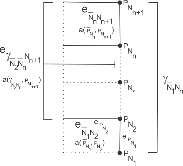
Figure 1: Timelike Curve in Quantum Spacetime.

In this way, as $n$ advances, we can interpret this in the sense that the event $\mathsf{e}_{\overline{N}_{n+1}N_{n+2}}$ is more “far away” from $\mathsf{e}_{\overline{N}_{1}N_{2}}$ in terms of proper time along the quantum timelike curve defined by the succession of the events $\mathsf{e}_{\overline{N}_{1}N_{2}}$ to $\mathsf{e}_{\overline{N}_{n+1}N_{n+2}}$.

 

Now, if we experience an elementary process, then, since there aren’t any “instants” of time “in the middle”, we would simply age a finite amount of time abruptly; that is, there’s a change, which, by itself, doesn’t introduce any extra proper time, the latter, instead, being fully accounted by the metric of the event and given “all at once”, as a photon gives all of its finite energy to an electron in an atom all at once. In the case of the previous elementary, “would be compound” events $\mathsf{e}_{\gamma_{\overline{N}_{2}\overline{N}_{n}}N_{n+1}}$, if there’s something like a particle in some of the intermediate events, then, if the system undergoes the elementary process $\mathsf{e}_{\gamma_{\overline{N}_{2}\overline{N}_{n}}N_{n+1}}$, it never interacts with the particle, it just “tunnels it”$.\,\blacksquare$

 

Before continuing, we will take $\theta(\overline{P}_{N_{1}},\overline{P}_{N_{2}})\equiv\theta$, in order to simplify the notation.

 

In the classical case, the time evolution in phase space is a map $t\,\longmapsto\phi_{t}^{*}s_{0}$. Here we define it in the same way, but now, since the states/events are pure states in a Hilbert space, we can also form linear combinations among them, and this invariably will bring typical quantum behaviour to the system (in a classical commutative algebra, the only pure states are the Dirac measures on the corresponding topological space, and linear combinations give mixed states, which cannot be interpreted as events in that case.) In the limit $\theta\,\longrightarrow\infty$ (we enter the macroscopic realm there), we will take a suitable boundary condition so that we recover the classical-like evolution curve.

 

$\mathbf{Definition\;2.22}$: Consider now the real valued functions $G(\theta)$ and $g(G(\theta))$. Then, the $\underline{\widetilde{\psi}^{\theta}}_{\overline{N}_{2}N_{3}}$ corresponding to the process $\mathsf{e}_{\overline{N}_{1}N_{2}}\bigcup\mathsf{e}_{\overline{N}_{2}N_{3}}$ (i.e., the event $\mathsf{e}_{\overline{N}_{2}N_{3}}$, but now seen as the endpoint of the considered path defined as $\mathsf{e}_{\overline{N}_{1}N_{2}}\bigcup\mathsf{e}_{\overline{N}_{2}N_{3}}$, or, equivalently, as the start of $\mathsf{e}_{\overline{N}_{3}N_{4}}$), is given by

$$\underline{\widetilde{\psi}^{\theta}}_{\overline{N}_{2}N_{3}}\doteq\phi_{\theta}(\underline{\psi}_{\overline{N}_{1}N_{2}})\doteq g(G(\theta))\underline{\psi}_{\overline{N}_{1}N_{2}}+G(\theta)(\underline{\psi}_{\overline{N}_{2}N_{3}}+\underline{I}),$$

where $\phi_{\theta}$ is continuous, with

$$G(0)=0,\,G^{\prime}(0)\neq 0,\,g(0)=1.\,\blacksquare$$

 

Thus,

$$\underline{\widetilde{\psi}^{0}}_{\overline{N}_{2}N_{3}}=\phi_{0}(\underline{\psi}_{\overline{N}_{1}N_{2}})=\underline{\psi}_{\overline{N}_{1}N_{2}},$$

that is, if $\theta=0$, then it makes no sense to distinguish between both events, they must be the same; furthermore, in light of this, the process and path for the classical case, in which $\theta\,\longrightarrow\infty$, should correspond to $\underline{\widetilde{\psi}^{\infty}}_{\overline{N}_{2}N_{3}}=\underline{\psi}_{\overline{N}_{2}N_{3}}$.

 

$\mathbf{Definition\;2.23}$: Now that we have two events, $\mathsf{e}_{\overline{N}_{1}N_{2}}$ and $\mathsf{e}_{\overline{N}_{2}N_{3}}$, we can calculate the transition probability between the events when following a particular path in spacetime given by the process $\mathsf{e}_{\overline{N}_{1}N_{2}}\bigcup\mathsf{e}_{\overline{N}_{2}N_{3}}$, which we define, as

$$\mathcal{P}_{\mathsf{e}_{\overline{N}_{1}N_{2}}\rightarrow\mathsf{e}_{\overline{N}_{3}N_{4}}^{start}}(\theta)^{\frac{1}{2}}\doteq(\underline{\widetilde{\psi}}_{\overline{N}_{2}N_{3}}^{\theta},\underline{\psi}_{\overline{N}_{1}N_{2}})_{\mathcal{H}_{\omega}}=g(G(\theta))\parallel\underline{\psi}_{\overline{N}_{1}N_{2}}\parallel_{\mathcal{H}_{\omega}}^{2}+$$

$$G(\theta)(\underline{\psi}_{\overline{N}_{2}N_{3}},\underline{\psi}_{\overline{N}_{1}N_{2}})_{\mathcal{H}_{\omega}}+G(\theta)(\underline{I},\underline{\psi}_{\overline{N}_{1}N_{2}})_{\mathcal{H}_{\omega}}$$

$$=g(G(\theta)).\,\blacksquare$$

 

In the classical situation, we have

$$\mathcal{P}_{\mathsf{e}_{\overline{N}_{1}N_{2}}\rightarrow\mathsf{e}_{\overline{N}_{3}N_{4}}^{start}}^{Class.}\doteq\mid(\underline{\psi}_{\overline{N}_{1}N_{2}},\underline{\psi}_{\overline{N}_{2}N_{3}})_{\mathcal{H}_{\omega}}\mid^{2}\,\mathrm{or}\,\mid(\underline{\psi}_{\overline{N}_{1}N_{2}},\underline{\psi}_{\overline{N}_{1}N_{2}})_{\mathcal{H}_{\omega}}\mid^{2},$$

and then we get only two possible values for the transition probability, namely, $0$ or $1$, respectively.

 

$\mathbf{Remark\;2.14}$: The map $\phi_{\theta}$ can be seen as the equivalent, in this formalism, of (the push-forward of) a $1-$parameter family of diffeomorphisms, and $\phi_{\theta}(\underline{\psi}_{\overline{N}_{1}N_{2}})$ can be seen as the “potential time evolution” in the phase space picture for the current quantum theory. Nevertheless, the physical interpretation is quite different. Indeed, in standard quantum physics, a well defined (by the true Hamiltonian with respect to a background spacetime geometry) and unique time evolution gives the state of the system at time $t$. Here, we don’t even have a “time $t$” to begin with: what $\phi_{\theta}(\underline{\psi}_{\overline{N}_{1}N_{2}})$ actually represents is, for a given possible time $\theta$, a possible time evolution itself to it, that is, in this situation, the different time evolutions (where what varies among them is the value of $\theta$) themselves are the ones which have different probabilities of occurring for the always fixed pair of “manifold points”/state supports $\underline{\psi}_{\overline{N}_{1}N_{2}}$ and $\underline{\psi}_{\overline{N}_{2}N_{3}}$. In this way, $\mathcal{P}_{\mathsf{e}_{\overline{N}_{1}N_{2}}\rightarrow\mathsf{e}_{\overline{N}_{3}N_{4}}^{start}}(\theta)^{\frac{1}{2}}$ is the probability that, when the initial event $\mathsf{e}_{\overline{N}_{1}N_{2}}$ goes to the final $\mathsf{e}_{\overline{N}_{2}N_{3}}$ (whose end sits at time $\theta+\theta_{12}$ from $\mathsf{e}_{\overline{N}_{1}N_{2}}$: since we have only two events here, $\theta$ can only take that value, besides $0$, of course), it will do it via the time evolution $\phi_{\theta}(\underline{\psi}_{\overline{N}_{1}N_{2}})$. Note that $\phi_{\theta}(\underline{\psi}_{\overline{N}_{1}N_{2}})$ doesn’t represent the state after the evolution, i.e., $\underline{\psi}_{\overline{N}_{2}N_{3}}$, it’s more than that, $\mathcal{P}_{\mathsf{e}_{\overline{N}_{1}N_{2}}\rightarrow\mathsf{e}_{\overline{N}_{3}N_{4}}^{start}}(\theta)^{\frac{1}{2}}$ is the probability that $\underline{\psi}_{\overline{N}_{1}N_{2}}$ quantum jumps/transitions to $\phi_{\theta}(\underline{\psi}_{\overline{N}_{1}N_{2}})$, which is the state in which a given time evolution (seen as some particular change or process) defines and in which event $\mathsf{e}_{\overline{N}_{2}N_{3}}$ has probability $1$ for ocurring, so that time actually acquires the value $\theta$, and then, since the notion of time evolution as something giving the state of the system at a defined time can make sense, can be reinterpreted as an evolution more similar to the one from standard quantum physics, in particular one which is such that the state at time $\theta$ is $\underline{\psi}_{\overline{N}_{2}N_{3}}$$.\,\blacksquare$

 

It remains to determine the functions $g,G$. For this, we will consider the dynamics as encoded in the spectral action. The spectral action on the NC $4-$Torus is given by ([9])

$$S^{0}=\omega(F_{\mu\nu}F^{\mu\nu}),$$

where

$$C^{\infty}(\mathbb{T}_{\Theta}^{4})\ni F_{\mu\nu}\doteq\delta_{\mu}(A_{\nu})-\delta_{\nu}(A_{\mu})+\left[A_{\mu},A_{\nu}\right],$$

and $C^{\infty}(\mathbb{T}_{\Theta}^{4})\ni A_{\mu}=-A_{\mu}^{*}$.

 

$\mathbf{Definition\;2.24}$: We define the following “displaced” version of the previous spectral action (we restrict $A_{\mu}$ to be only from any of the two algebras of the two events in consideration, since that’s where the action of $\phi_{\theta}$ was defined)

$$S^{\theta}\doteq\omega(\phi_{\theta}(F_{\mu\nu}F^{\mu\nu}))=g(G(\theta))S^{0}+G(\theta).\,\blacksquare$$

 

$\mathbf{Hypothesis\;2.3}$: We impose its invariance (because the $\phi_{\theta}$ are the analogous of physical diffeomorphisms) on the variable $\theta$:

$$\frac{\mathrm{d}S^{\theta}}{\mathrm{d}\theta}=0.\,\blacksquare$$

 

$\mathbf{Lemma\;2.8}$: Hypothesis 2.3 implies that $g(G(\theta))_{S^{0}}=1-\frac{1}{S^{0}}G(\theta)$.

 

Proof:

$$\frac{\mathrm{d}S^{\theta}}{\mathrm{d}\theta}=\frac{\mathrm{d}g}{\mathrm{d}\theta}S^{0}+\frac{\mathrm{dG}}{\mathrm{d}\theta}$$

$$0=\frac{\mathrm{d}g}{\mathrm{d}G}\frac{\mathrm{d}G}{\mathrm{d}\theta}S^{0}+\frac{\mathrm{d}G}{\mathrm{d}\theta}\,\Longrightarrow 0=\frac{\mathrm{d}g}{\mathrm{d}G}S^{0}+1\,\Longrightarrow$$

$$g(G(\theta))_{S^{0}}=k-\frac{1}{S^{0}}G(\theta),$$

with $k=1$, since $G(0)=0$ and $g(0)=1$. In this way:

$$g(G(\theta))_{S^{0}}=1-\frac{1}{S^{0}}G(\theta).\,\square$$

 

Now, consider the case for the solution $A_{\mu}^{0}=0$, then $S^{\theta}(A_{\mu}^{0})$ cannot be invariant on $\theta$, and, in fact (recall that $G^{\prime}(0)\neq 0$):

$$S^{\theta}(A_{\mu}^{0})=G(\theta);$$

each value of $\theta$ corresponds to a different physical situation (roughly speaking, in the semiclassical case, the second event varies its temporal “distance” with respect to the initial one as $\theta$ varies); thus, the three action values $S^{\theta_{1}}(A_{\mu}^{0}),$ $S^{\theta_{2}}(A_{\mu}^{0})$, $S^{\theta_{1}+\theta_{2}}(A_{\mu}^{0})$, correspond to three different physical systems.

 

$\mathbf{Hypothesis\;2.4}$: We propose that the dynamics of these systems under the $\theta$ variable varies in a homogeneous and additive fashion, that is (recall that the sum of actions corresponds to the composition or physical sum of physical systems),

$$S^{\theta_{1}+\theta_{2}}(A_{\mu}^{0})=S^{\theta_{1}}(A_{\mu}^{0})+S^{\theta_{2}}(A_{\mu}^{0})\,\Longrightarrow$$

$$G(\theta_{1}+\theta_{2})=G(\theta_{1})+G(\theta_{2}).$$

If $G$ is continuous, then this implies that

$$G(\theta)=\alpha\theta,$$

for some constant $\alpha=G^{\prime}(0)\neq 0$ (not that this is valid for any solution $A_{\mu}$, since $G$ only depends on $\theta$)$.\,\blacksquare$

 

$\mathbf{Corollary\;2.1}$: The final form, completely determined by the toral spectral action and our assumptions, of the transition probability becomes

$$\mathcal{P}_{\mathsf{e}_{\overline{N}_{1}N_{2}}\rightarrow\mathsf{e}_{\overline{N}_{3}N_{4}}^{start}}(\theta)_{\alpha,A_{\mu}}^{\frac{1}{2}}=1-\frac{\alpha}{S^{0}(A_{\mu})}\theta.\,\square$$

 

$\mathbf{Remark\;2.15}$: From the form of the toral algebra $\mathcal{\widehat{A}}_{\overline{P}_{N_{1}}\overline{P}_{N_{2}}}$, where $u_{1}u_{3}=e^{2\pi i\theta}u_{3}u_{1}$, it’s clear that a redefinition of $\theta$ by a displacement $\theta\,\longmapsto\theta+n$, with $n\in\mathbb{N}$, gives an isomorphic algebra; thus, we can restrict to $\theta\in\left[0,1\right]$. Furthermore, the map defined by $u_{1}\,\longmapsto u_{3}$ and $u_{3}\,\longmapsto u_{1}$ establishes an isomorphism between the toral algebra with $\theta$ and the one with $1-\theta$; if we combine both of these results, then we get that the family of toral algebras whose parameter $\theta$ ranges on the subset $\left[0,\frac{1}{2}\right]$ exhausts all the possible non-isomorphic toral algebras (for the $2-$dimensional case, of course.) In this way, if we impose the only physically meaningful boundary condition, namely,

$$lim_{\theta\longrightarrow\frac{1}{2}}\underline{\widetilde{\psi}^{\theta}}_{\overline{N}_{2}N_{3}}\propto(\underline{\psi}_{\overline{N}_{2}N_{3}}+\underline{I}),$$

which is equivalent to asking

$$lim_{\theta\longrightarrow\frac{1}{2}}g(G(\theta))_{S^{0}(A_{\mu})}^{\alpha}=lim_{\theta\longrightarrow\frac{1}{2}}\mathcal{P}_{\mathsf{e}_{\overline{N}_{1}N_{2}}\rightarrow\mathsf{e}_{\overline{N}_{3}N_{4}}^{start}}(\theta)_{\alpha,A_{\mu}}=0,$$

then, for each solution $A_{\mu}$, there’s a unique solution

$$g(G(\theta))_{S^{0}(A_{\mu})}^{\alpha_{\frac{1}{2}}}=1-2\theta$$

to the displaced dynamics, obtained by taking

$$\alpha_{\frac{1}{2}}=2S^{0}(A_{\mu}).$$

For this case, the graph of $\mathcal{P}_{\mathsf{e}_{\overline{N}_{1}N_{2}}\rightarrow\mathsf{e}_{\overline{N}_{3}N_{4}}^{start}}(\theta)_{\alpha_{\frac{1}{2}},A_{\mu}}$ is, of course, just the following:

                                          

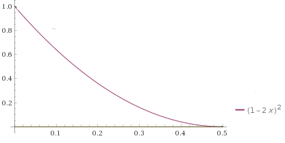
Figure 2: Transition Probability for $\alpha_{\frac{1}{2}}$$.\,\blacksquare$

 

$\mathbf{Remark\;2.16}$: In the unexponentiated algebra, one would like to have non-isomorphic algebras for any value of the parameter $\theta$ in the range $[0,\infty)$. Thus, in the exponentiation of the algebra, we made an unintended compactification of $[0,\infty)$ into $\left[0,\frac{1}{2}\right]$. To obtain the actual domain and shape of the transition probability, we must change the variable $\theta$ to $\vartheta\in[0,\infty)$, where the passing from $\theta$ to $\vartheta$ is given by a bijective conformal stretching of $[0,\frac{1}{2})$ into $[0,\infty)$. The most sensible option seems to be:

$$\theta=\frac{1}{2}\mathrm{tanh}\,\vartheta,$$

in which case

$$\mathcal{P}_{\mathsf{e}_{\overline{N}_{1}N_{2}}\rightarrow\mathsf{e}_{\overline{N}_{3}N_{4}}^{start}}(\vartheta)_{\alpha_{\frac{1}{2}},A_{\mu}}=(1-\mathrm{tanh}\,\vartheta)^{2}$$

$$=e^{-4\vartheta}(1+\mathrm{tanh}\,\vartheta)^{2};$$

now, for $\vartheta>>4$, this reduces to

$$\mathcal{P}_{\mathsf{e}_{\overline{N}_{1}N_{2}}\rightarrow\mathsf{e}_{\overline{N}_{3}N_{4}}^{start}}(\vartheta)_{\alpha_{\frac{1}{2}},A_{\mu}}\sim 4e^{-4\vartheta}.$$

 

Then the graph becomes:

                                          

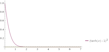
Figure 3: Transition Probability for $\alpha_{\frac{1}{2}}$ (conformally stretched)$.\,\blacksquare$

 

The state of the system is given by $\Psi=\underline{\psi}_{\overline{N}_{1}N_{2}}$, then it has non-zero transition probability for several other processes; that is, upon interaction with the surrounding matter fields, the initial state $\underline{\psi}_{\overline{N}_{1}N_{2}}$ can make a quantum jump to the start of another event $\underline{\psi}_{\overline{N}_{n+1}N_{n+2}}$ via an elementary, “would be compound” process $\mathsf{e}_{\gamma_{\overline{N}_{1}\overline{N}_{n}}N_{n+1}}$, which may even lie in a different curve $\gamma^{\prime}$ (see next figure), and this is the physical interpretation we give to $\mathcal{P}_{\mathsf{e}_{\overline{N}_{1}N_{2}}\rightarrow\mathsf{e}_{\overline{N}_{n+1}N_{n+2}}^{start}}(\mathrm{a}(\gamma_{\overline{N}_{2}\overline{N}_{n}},P_{N_{n+1}}))_{\alpha_{\frac{1}{2}},A_{\mu}}$. We also note that, unlike the classical case, we don’t need to introduce change in an ad-hoc manner here, since change can be seen as arising from quantum collapse (now taken as ontologically fundamental and irreducible) after an interaction. We take the collapse as the only source of change and actually identify it with it (in other views, collapse, of course, implies change, but the converse is not necessary; here we say they are indeed the same thing.) Thus, the change in the classical theory actually comes from the fundamental quantum theory, of which the former is a limit. Furthermore, in light of this, then the argument used to show the necessity of the collapse in QM can be now used to show the necessity of change, which then becomes a quantum phenomena and very tied to the characteristic non-commutativity of quantum properties.

 

                                                

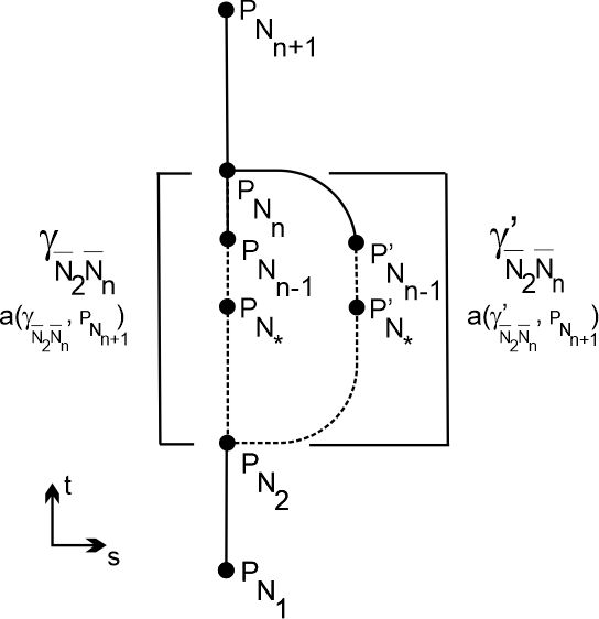
Figure 4: Two Different Curves.

 

In the actual physical reality, the system is constantly interacting and its state collapsing. Therefore, its real spacetime trajectory is something like what’s illustrated in the figure below (note that not all of the intermediate events in the curves $\gamma_{\overline{N}_{1}\overline{N}_{n}}$ are visited, i.e., not all the intermediate values of process-area will be visited.) It’s actually for this trajectory that we can define something like

$$m\,\longmapsto\mathrm{a}(\gamma_{\overline{N}_{2}\overline{N}_{n(m)}},P_{N_{n(m)+1}})\,\longmapsto\mathsf{e}(\mathrm{a}(\gamma_{\overline{N}_{2}\overline{N}_{n(m)}},P_{N_{n(m)+1}}))\equiv\mathsf{e}_{\overline{N}_{n(m)+1}N_{n(m)+2}}^{start},$$

as in the classical $t\,\longmapsto$$\tau(t)\,\longmapsto\gamma(\tau(t))$.

                                                

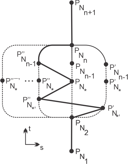
Figure 5: Real Spacetime Trajectory of the System.

 

$\mathbf{Remark\;2.17}$: The so-called Problem of Time can be resolved here simply by calculating the values of the properties of interest (say, the spatial curvature) on each of the nodes of $\mathsf{e}(\mathrm{a}(\gamma_{\overline{N}_{2}\overline{N}_{n(m)}},P_{N_{n(m)+1}}))$. Of course, since quantum collapse is random, we cannot predict with certainty what’s the trajectory that the system will take, and thus the precise time evolution of the value for the property being considered. The only thing we can do is to calculate the probability for each possible time evolution of the value, by setting:

$$\mathcal{P}(m)\doteq\prod_{k=1}^{m}\mathcal{P}_{n(k),n^{\prime}(k)}^{spatial}\mathcal{P}_{\mathsf{e}_{\overline{N}_{n(k)}N_{n(k)+1}}\rightarrow\mathsf{e}_{\overline{N}_{n^{\prime}(k)+1}N_{n^{\prime}(k)+2}}^{start}}(\mathrm{a}(\gamma_{\overline{N}_{n(k)+1}\overline{N}_{n^{\prime}(k)}},P_{N_{n^{\prime}(k)+1}}))_{\alpha_{\frac{1}{2}},A_{\mu}},$$

where only the events in $\mathsf{e}(\mathrm{a}(\gamma_{\overline{N}_{2}\overline{N}_{n(m)}},P_{N_{n(m)+1}}))$ are considered for the product$.\,\blacksquare$

 

$\mathbf{Remark\;2.18}$: Now, since $\mathcal{P}_{\mathsf{e}_{\overline{N}_{1}N_{2}}\rightarrow\mathsf{e}_{\overline{N}_{n+1}N_{n+2}}^{start}}(\mathrm{a}(\gamma_{\overline{N}_{2}\overline{N}_{n}},P_{N_{n+1}}))_{\alpha_{\frac{1}{2}},A_{\mu}}$ falls exponentially, then the events $\mathsf{e}_{\gamma_{\overline{N}_{2}\overline{N}_{n}}N_{n+1}}$ for large $n$ are very unlikely to happen. This means that $\mathsf{e}_{\overline{N}_{1}N_{2}}$ tends to go to a $\mathsf{e}_{\overline{N}_{n+1}N_{n+2}}^{start}$ which is closer to it in proper time separation. Physically, this means that time advances as a succession of instants which are very close to each other in proper time distance and in which the duration of the instants themselves is very small. Thus, at the macroscopic scale, this is perceived as a succession of instants, each of duration zero, which forms a continuum whose subsets have finite duration, and which monotonically increases (since, upon change, almost all intermediate steps are visited, and, thus, the system can interact with whatever thing that resides at those steps), that is, the classical picture of time. The quantum system at an event is surrounded by a dispersion cloud of events which can visit next, and the classical proper time is just some average $<\tau>$ of that dispersion, and the actual quantum transitions measure how much the actual quantum time deviates from this average $<\tau>$$.\,\blacksquare$

 

$\mathbf{Remark\;2.19}$: Also in relation to this, this point of view may also shed some light on the so-called Measurement Problem of standard QM, understood as the impossibility to explain the collapse of the wavefunction in terms of the standard Schrödinger time evolution (assuming that the collapse gives definite values and that standard QM is complete.) Indeed, in our view, the standard classical time, which, among other things, is used as the external time parameter to define the Schrödinger time evolution, is only an emergent feature at the macro level, and fuelled at the micro, fundamental level by an irreducible collapse. Thus, the Schrödinger time evolution will break when something from the fundamental level leaks to the macroscopic level. And, of course, this is precisely the situation in a quantum measurement, when the state collapses when certain two systems interact: the classical time will never be able to explain this process since the latter intervenes precisely in making possible the quantum, and therefore also the classical, time. Finally, one can also may be able to avoid spacetime singularities (the “Singularity Problem” of classical GR) in this approach thanks to the discretization of time and the mentioned “tunneling” effect. Indeed, the discretization eliminates the possibility for a property to acquire values which are finite yet arbitrary large as one approaches an event separated by a finite amount of proper time (either to the past or future) with respect to the initial one, since there are only a finite number of other events between them, thus the property reaches a finite maximum value, possibly at the final event; furthermore, if the property is not defined for an event, then, of course, it cannot form part of the spacetime, yet, due to the possibility of tunneling, even if the classical spacetime is inextendible, there still exists a non-zero transition probability for the system to tunnel to an extended quantum spacetime, that is, beyond the “boundary” of the classical spacetime defined by the singularity$.\,\blacksquare$

 

3. Discussion

 

In CLQG (Covariant LQG [13]), given the Hilbert spaces and quantum algebras at the boundary, it seems one can only calculate things like (quantum) properties of the induced spatial $3-$d metric (areas, volumes, curvature) and the extrinsic curvature of the hypersurface, and not quantum durations (for example, in the analysis done for the extrinsic coherent states, the area and the extrinsic curvature peak at those states, but time is introduced as an already peaked external parameter.) There are some extensions that introduce timelike boundaries, but, for a time evolution, we need to be able to introduce durations also in the interior of the process; furthermore, the commutation relations for variables whose weight functions have a spacetime support, and in regions in spacetime that are such that one is in the causal future of the other, are non-trivial (this is the important result of the so-called covariant Poisson brackets), and are not accounted for by the part of the commutation relations that arise purely due to the structure (kinematical in nature) of the group in the Yang-Mills-like/connection variables used in these formulations [14], since the dependence over the causality comes from the hyperbolic character of the dynamics and the mentioned issue with the supports, and then it’s indifferent if we take the Yang-Mills/connection group to be $SU(2)$ (spacelike boundary) or $SU(1,1)$ (timelike boundary), that is, this causal part will be present even if the field variable were a scalar field; as argued in the paper, and from relational considerations, we consider this a key issue in the quantization of duration, which makes it quite different from the quantization of the spatial metric and that it cannot thus be completely obtained by tweaks on the already existing methods for the latter. In particular, the extensions of CLQG give the area of a timelike triangle for vectors (one timelike and the other spacelike) whose origin is at the same vertex (evidently, the causal part is irrelevant, since the origin of both vectors is the same point, and then only the group part enters to play there), while TQG describes the same area but from the point of view of the causal connection between the initial and enpoint of the timelike vector (thus, the causal part is relevant for that); both refer to a same event and as a finite process, but TQG gives a more dynamical characterization of it while CLQG gives its internal kinematical degrees of freedom. Thus, the corresponding quantum algebra for duration is a composition of the group and causal aspect of the classical Poisson bracket. From this causal part, unique to TQG, one gets an universal decay for the transition that explains the features of duration at the macro scale (this decay is always there and is independent of the details of the other parts of the transitions); this part of the transition for duration is ignored (or considered to have already peaked) in treatments that rely heavily in coherent states adapted only to the group part.

 

In classical GR, the full form of a solution is $g_{ab}=n_{a}n_{b}+h_{ab}$, with $n^{a}=\frac{1}{N}(t^{a}+N^{a})$, where $N$ and $N^{a}$ are, respectively, the lapse and shift (which also satisfy $N=-g_{ab}n^{a}t^{a}$ and $N^{a}=h_{b}^{a}t^{b};$ in this way, $N$ is interpreted as the “rate of proper time with respect to coordinate time $t$ as one moves normaly to the hypersurfaces of the foliation”), so that the proper time becomes $\tau=\int\sqrt{N^{2}-h_{ab}N^{a}N^{b}}\,\mathrm{d}t$. Now, it’s also known that the induced metric and the extrinsic curvature (the data given by the boundary Hilbert spaces and algebras of CLQG) determine a point in phase space if we were in the classical theory. But this is not enough to generate a solution, one also needs to specify the lapse and shift $N$ and $N^{a}$ (which measure how the time function/coordinate $t$ of the foliation $\varSigma_{t}$ of the manifold interacts with the metric information.) Furthermore, from the previous formulas we can see that the lapse and shift $N$ and $N^{a}$ are precisely the things that encode the time part/time evolution of the spacetime behaviour of the solution, as well as the proper time (we just can’t have one without the other.) Therefore, in order to describe time evolution properly, we must introduce some extra information to CLQG, which is given by an algebra that can econde the non-trivial commutation relations between causally connected regions in spacetime in the interior of the process (and find a way to describe metric properties related to it.) But, even if we have this, the transition amplitude $W(x_{i},x_{f})$ is not useful for obtaining the amplitude for the transitions between quantum states of duration, since it’s based on the path integral, which, as one can see in the canonical framework, involves integration over all lapse functions $N$, and then information about the duration part of a particular solution cannot be taken as being prescribed from there. Thus, the dynamical transitions for duration must also be provided by different means. TQG provides both of these necessary ingredients for the adequate description of time evolution in QG (the areas of the elementary processes in the paper can be interpreted as the information provided by $N$ and $N^{a}$ in the classical case.)

 

The probabilty amplitude $\mid W(x_{i},x_{f})\mid^{2}$ of CLQG should, perhaps, be interpreted as what is denoted as $\mathcal{P}_{n(k),n^{\prime}(k)}^{spatial}$ here. On the other hand, TQG, by providing an actual description of time duration in QG, is what actually justifies the physical interpretation of $W(x_{i},x_{f})$ as a transition amplitude in CLQG, the latter is a thing which has often been criticized ([2]) due to the integration over all lapse functions on the path integral: if we delegate the time part to TQG, then this integration can be seen only as a device of the calculation, since no contradiction arises because the path integrals are being applied to states that only describe space and to obtain the pure space part of the transition amplitude.

 

Thus, we actually see CLQG and TQG as complementary theories.

 

4. Conclusions

 

We made a schematic partial quantization of the temporal part in line with the mentioned ideas. For doing that, we had to introduce a new formalism for QG, which we call TQG, since it’s heavily based on the NC Tori. This allowed us to obtain numerous insights about the nature of time, like its discretization, its regular pace at the macroscopic scale, a solution to the Problem of Time, and a connection with the Measurement Problem of QM.

 

TQG is not that much a theory of quantum gravity, but a necessary part of it. In particular, it provides a basic framework on which to discuss within such a theory any aspect related to time, time evolution, and duration. In this proposal, the part of quantum phase space that deals with these aspects is modeled by an $n-$dimensional noncommutative Torus, where each state on a NC-2-subTorus there corresponds to an elementary and irreducible quantum process in a spacetime picture; the NC-Torus arises here because for, say, three (of four) elements that are causally related, one needs three generators that do not commute among each other (this comes from the canonical quantization of the Poisson brackets of phase space properties with weight functions having causally connected supports), and this cannot be accomodated just in the product of two NC-2-Torus (that model an individual quantum elementary process), but one needs a missing third non-commutation between these two, so to speak, and this can be done in the general $3$ and $4-$NC-Torus. This type of phase space hasn’t been discussed in any of the current proposal for quantum gravity theories, despite the fact that often some talk is informally given ([15, 4]) about the behaviour of quantum time (like its hypothetical quantum nature, with superpositions, etc.), that, really, can only be properly justified if one has a model for this phase space.

References

- [1] Wald, R.M. (1984). General Relativity (The University of Chicago Press, Chicago); Wald, R.M. (1994). Quantum Field Theory in Curved Spacetime and Black Hole Thermodynamics (Chicago Lectures in Physics. University Of Chicago Press).
- [2] Thiemann, T. (2008). Modern Canonical Quantum Gravity (Cambridge University Press; 1 edition).
- [3] a) Connes, A. (1995). Noncommutative Geometry (Academic Press, San Diego); b) Connes, A. (2008). On the spectral characterization of manifolds (URL https://arxiv.org/abs/0810.2088); c) Connes, A.; Marcolli, M. (2008). Nonconmmutative Geometry, Quantum Fields and Motives (Colloquium Publications, American Mathematical Society, Providence, United States); d) van Suijlekom, W. (2015). Noncommutative Geometry and Particle Physics (Springer); e) Gracia-Bondía, J.M.; Várilly, J.C.; Figueroa, H. (2001). Elements of Noncommutative Geometry (Birkhäuser, Basel); f) Várilly, J.C. (2006). Dirac Operators and Spectral Geometry (Lecture Notes; URL https://www.impan.pl/swiat-matematyki/notatki-z-wyklado~/varilly_dosg.pdf).
- [4] Rovelli, C. (2007). Quantum Gravity (Cambridge Monographs on Mathematical Physics).
- [5] Strocchi, F. (2005). An Introduction To The Mathematical Structure Of Quantum Mechanics: A Short Course For Mathematicians (World Scientific, Singapore); Landsman, N.P. (2017). Foundations of Quantum Theory (Springer); Moretti, V. (2013). Spectral Theory and Quantum Mechanics: With an Introduction to the Algebraic Formulation, UNITEXT, vol. 64 (Springer-Verlag, Berlin); Khavkine, I.; Moretti, V. (2015). Algebraic QFT in Curved Spacetime and quasifree Hadamard states: an introduction (URL https://arxiv.org/abs/1412.5945).
- [6] Fathizadeh, F.; Khalkhali, M (2019). Curvature in Noncommutative Geometry (URL https://arxiv.org/abs/1901.07438).
- [7] Khavkine, Igor (2012). Characteristics, Conal Geometry and Causality in Locally Covariant Field Theory (URL https://arxiv.org/abs/1211.1914).
- [8] Henson, J. (2009). The causal set approach to Quantum Gravity (Approaches to Quantum Gravity; Daniele Oriti, editor; Cambridge University Press).
- [9] Eckstein, M.; Iochum, B. (2018). Spectral Action in Noncommutative Geometry (SpringerBriefs in Mathematical Physics vol. 27).
- [10] Rovelli, C. (2018). “Space is blue and birds fly through it” (URL https://arxiv.org/abs/1712.02894).
- [11] Choquet-Bruhat, I. (2008). General Relativity and the Einstein Equations (Oxford Mathematical Monographs).
- [12] Ascárate, A. (2020). The Spacetime Picture in Quantum Gravity (URL https://arxiv.org/abs/2012.03994).
- [13] Rovelli, C.; Vidotto, F. (2014). Covariant Loop Quantum Gravity : An Elementary Introduction to Quantum Gravity and Spinfoam Theory (Cambridge University Press).
- [14] Conrady, F.; Hnybida, J. (2010). A spin foam model for general Lorentzian 4-geometries. Class. Quantum Grav. 27 185011 (preprint: URL https://arxiv.org/abs/1002.1959v4).
- [15] Rovelli, C. (2021). The layers that build up the notion of time (Contribution to the volume ’Time and Science’, R. Lestienne and P. Harris eds., World Scientific).