FOSSIL: I. The Spin Rate Limit of Jupiter Trojans

Abstract

Rotation periods of 53 small (diameters $2~{}\mathrm{km}<D<40$ km) Jupiter Trojans (JTs) were derived using the high-cadence light curves obtained by the FOSSIL phase I survey, a Subaru/Hyper Suprime-Cam intensive program. These are the first reported periods measured for JTs with $D<10$ km. We found a lower limit of the rotation period near 4 hr, instead of the previously published result of 5 hr (Ryan et al., 2017; Szabó et al., 2017, 2020) found for larger JTs. Assuming a rubble-pile structure for JTs, a bulk density of $\approx$0.9 g cm^-3 is required to withstand this spin rate limit, consistent with the value $\sim 0.8-1.0$ g cm^-3 (Marchis et al., 2006; Mueller et al., 2010; Buie et al., 2015; Berthier et al., 2020) derived from the binary JT system, (617) Patroclus–Menoetius system.

1 Introduction

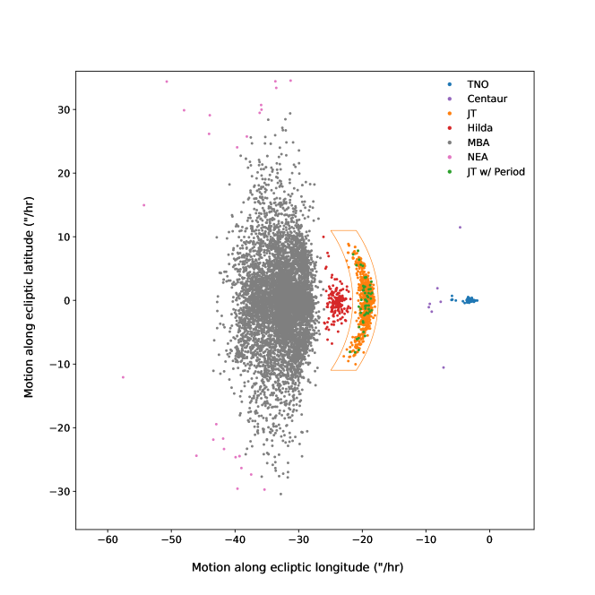
Figure 1: Motions along the ecliptic longitude and latitude of the moving objects detected in the FOSSIL observations. The moving objects are classified as outlined in Yoshida & Terai (2017). The JTs discussed in this paper are indicated by orange dots, and the JTs with fit rotation periods are indicated in green.

The FOSSIL Survey (Formation of the Outer Solar System: An Icy Legacy) is an intensive survey program using Subaru/Hyper Suprime-cam (HSC). The goal of the program is to measure the populations and characteristics of Jupiter Trojans (JTs) and the various dynamical sub-populations of the small bodies in the Trans-Neptunian region. The results of this survey program will provide important clues to our understanding of the formation and evolution of our Solar System. A major scientific goal of the initial phase of the survey is to obtain high-cadence lightcurves of small JTs and measure their rotation periods.

Table 1: Details of the observations for each survey block.

Block	RA	Dec	JT	Number of	Filter	Exposure	Limiting	Cadence	Date	Exposures	Time
ID	(deg)	(deg)	Cloud	Pointings		Time (s)	Magnitude	(min)		per Pointing	Span (hr)
19Apr	197.526	-6.763	L5	5	$g$	90	24.5	10	2019-04-10	53	8.8
20May	224.351	-14.596	L5	2	$r2$	300	25.6	11	2020-05-19	23	3.8
							25.7		2020-05-20	21	3.8
20Aug	341.656	-6.039	L4	3	$r2$	300	25.6	16	2020-08-21	16	4.5
							25.6		2020-08-22	15	4.0
							25.5		2020-08-23	15	4.1
20Oct	10.119	5.754	L4	3	$r2$	150	25.5	15	2020-10-14	24	3.4
							25.4		2020-10-15	24	3.4
							24.0		2020-10-16	8	1.0
							24.0		2020-10-17	8	1.0

JTs are a population of asteroids co-orbiting with Jupiter near its L4 and L5 Lagrangian points. Because the orbits of JTs are relatively stable, it is believed that their properties hold important information about the primitive Solar System. JTs could have been formed at their present locations during the formation of Jupiter (Marzari & Scholl, 1998; Fleming & Hamilton, 2000), or they formed somewhere else during the early stages of the solar system formation and were then captured into their current locations as Trojans during migration of the giant planets (Fernandez & Ip, 1984; Malhotra, 1995; Morbidelli et al., 2005; Lykawka & Horner, 2010; Nesvorný et al., 2013). Comparative studies of the overall physical properties between JTs and other small body populations are crucial to our understanding of the origin of JTs and the formation of our solar system.

A significant amount of previous work has been completed in order to better understand the JT population. Two major spectral groups, i.e., red (D-type) and less red (P-type), have been identified within this population (Emery et al., 2011; Wong et al., 2014; Wong & Brown, 2015) . However, it is not clear how this color bi-modality is related to other small body populations in the solar system which also have dichotomous colors. Although the size distribution of JTs is different from that of the Main Belt Asteroids (MBAs) (Yoshida & Terai, 2017), this difference could be a result of either different primordial origins or different evolutionary histories. Finally, several measurements of the JT binary fraction have been reported (Mann et al., 2007; Sonnett et al., 2015; Ryan et al., 2017; Szabó et al., 2017; Nesvorný et al., 2020), but this value is very uncertain, with estimates in the range of 10% to 30%

The bulk densities and interior structures of JTs will also provide useful insight when compared with other small body populations. In addition to probing these properties for individual objects through space missions or binary searches, overall estimations can be made through their common spin-rate limit which can be identified from a rotation period survey. Thanks to the availability of wide-field cameras, this application has been extensively used on MBAs in the past few years. It is believed (Chapman, 1978; Davis et al., 1985; Weissman, 1986) that MBAs with diameters $1~{}\mathrm{km}\lesssim D\lesssim 100$ km are gravitational aggregates (rubble-pile structures). These asteroids can thus be destroyed if they spin too fast, and consequently have an upper limit for their spin rates. Harris (1996) first reported a 2 hr rotation period lower limit for MBAs of diameters $D>150$ m and suggested that these asteroids have rubble-pile structures with a lower limit on their bulk densities of $\sim$3 g cm^-3. This 2 hr rotation period limit has consistently been seen in more recent data sets (Masiero et al., 2009; Chang et al., 2015, 2016, 2019). Interestingly, more than two dozen super fast rotators (SFRs), asteroids with $D>300$ m and rotation periods $<2$ hr, have been found (see Chang et al., 2019, and references therein). Unless these objects have extremely high bulk densities, rubble-pile structures could not survive such high rotation rates, indicating cohesive force is required in addition to gravity to preserve the structures of these objects (Holsapple, 2007; Hirabayashi, 2015; Hu et al., 2021).

While the wide-field surveys for asteroid rotation periods referenced above have helped to understand their bulk densities and interior structures, this kind of survey has not been conducted for JTs. Ryan et al. (2017), Szabó et al. (2017, 2020) reported a possible rotation period lower limit of $\approx$5 hr for JTs using the K2 data set. However, their JT samples were limited to diameters $D>10$ km, and these relatively large JTs have probably not been accelerated by the Yarkovsky–OKeefe–Radzievskii–Paddack (YORP) effect (Rubincam, 2000) to reach their spin-rate limit.

To achieve this goal we used Subaru and HSC (Miyazaki et al., 2018; Komiyama et al., 2018; Kawanomoto et al., 2018; Furusawa et al., 2018) to conduct a wide-field survey, from which dense lightcurves with durations from 1 to 3 nights were collected to measure rotation periods for small JTs ($D\leq 10$ km). A total of 53 rotation periods were obtained by this survey.

This article is organized as follows. The observations, data reduction, and lightcurve extraction are described in Section 2. The rotation period analysis is discussed in Section 3. The results and discussion are presented in Section 4, and a summary is given in Section 5.

Table 2: Photometric Measurements for JT data presented in this paper.

JD	Mag	Mag Error
FASP03010029
(156294) 2001 WU66
2458583.857932	20.9790	0.0062
2458583.864924	20.9308	0.0061
2458583.885930	20.8650	0.0059
2458583.892958	20.8545	0.0058
2458583.900007	20.8459	0.0058
2458583.907036	20.8728	0.0059
2458583.914078	20.9097	0.0059
2458583.921106	20.9317	0.0060
2458583.928126	21.0006	0.0062
2458583.938686	21.0513	0.0065
2458583.945697	21.1222	0.0069
2458583.952704	21.2509	0.0070
2458583.959705	21.3866	0.0078
2458583.966701	21.4131	0.0078
2458583.973695	21.4045	0.0078
2458583.980718	21.3482	0.0080
2458583.987715	21.3897	0.0076
2458583.994707	21.3218	0.0074
2458584.001710	21.2038	0.0072
2458584.008693	21.0953	0.0070
2458584.015689	21.0485	0.0068
2458584.022678	20.9955	0.0068
2458584.029678	20.9469	0.0066
2458584.036667	20.9121	0.0065
2458584.043656	20.8892	0.0063
2458584.050641	20.8427	0.0062
2458584.057636	20.8129	0.0062
2458584.071627	20.8376	0.0063
2458584.078620	20.8561	0.0065
2458584.085612	20.8340	0.0067
2458584.092621	20.9180	0.0069
2458584.099606	20.9786	0.0070
2458584.106602	20.9651	0.0078
2458584.113589	21.0144	0.0079

Note. — This is an example for a single object; all measurements from all 53 objects are available in machine-readable format.

2 Observations and Data Reduction

High-cadence observations were performed on four blocks of pointings targeting the L4 and L5 JT clouds. The details of observations can be found in Table 1. Observations were conducted using Subaru/HSC during 2019 April 10 (19Apr), 2020 May 18–19 (20May), 2020 August 20–22 (20Aug), and 2020 October 13–16 (20Oct). The $g$-band filter was used for the 19Apr observations, and the $r2$-band was used for the other three blocks. The observation time spans were roughly 8 hr for 19Apr and 4 hr each night for the observations conducted in 2020 (other than the last two nights of the 20Oct block, where the time was reduced due to poor weather).

The 19Apr data is from a previous observing run, and was not part of the original FOSSIL proposal. However, given that everyone of the proposers for the 19Apr observations is a member of the FOSSIL collaboration, these data were combined with the FOSSIL data set.

FOSSIL was originally awarded four nights in both May (2020A) and September (2020B) when the L5 and L4 JT clouds, respectively, were at opposition. However, we lost three of our four nights of scheduled observations in 2020A because of the shutdown of Maunakea due to the COVID-19 pandemic, and our 2020B nights were rescheduled to August and October due to necessary Subaru maintenance which had been deferred due to the pandemic. The change in our observing schedule necessitated the cancellation of our planned JT color measurements, but we were still able to make useful JT lightcurve measurements during the time we managed to observe.

The number of selected pointings and the exposure time of each frame were adjusted for each block as we learned from our experience from the analysis of the previously observed blocks. For each block, exposures were cycled through the selected pointings repeatedly throughout each night. The typical limiting magnitudes were 24.5 mag for 19Apr and 25.4–25.7 mag for the others (except for the last two nights of the 20Oct block observations where the limiting magnitude dropped to 24 mag due to poor weather conditions). A total of 13 pointings were used, for a total sky coverage of 37.7 deg². Of this, 17.4 deg² covered the L4 cloud and 20.3 deg² covered L5.

All the images were processed using the official HSC pipeline, hscPipe v8.3 (Bosch et al., 2018), with astrometry and photometry calibrated against the Pan-STARRS 1 catalog (Chambers et al., 2017). For each pointing, hscPipe was used to build a template image in order to produce differential images. The differential images were then processed by the same pipeline to generate source catalogs of potential moving objects.

Since the observations were carried out using relatively long exposure times, the images of the moving objects with relatively short geocentric distance were trailed. In order to improve the photometry for the trailing moving objects, the trailed source fitting software package TRIPPy (Fraser et al., 2016a, b) was used to measure the magnitudes of the moving object candidates. For each CCD in the HSC focal plane, TRIPPy creates a point spread function (PSF) model for each exposure based on the PSFs from a subset of stars on the same chip. This PSF model is then used along with the measured rate of motion of the relevant JT to create a trailing aperture for the moving object. The background is calculated as the median pixel value in the differential image from a set of pixels separated from the trailed PSF based on the full width half maximum (FWHM) of the model PSF. An aperture correction based on the FWHM is then applied to the resulting photometric measurement. The intra-night detections of the moving objects would appear as linear sequences with correlated epochs. The Hough transform (Hough, 1959; Duda & Hart, 1972), an algorithm for line detection in images, was thus utilized to correlate the linear intra-night detections and find moving objects. This procedure is described in detail in Chang et al. (2019).

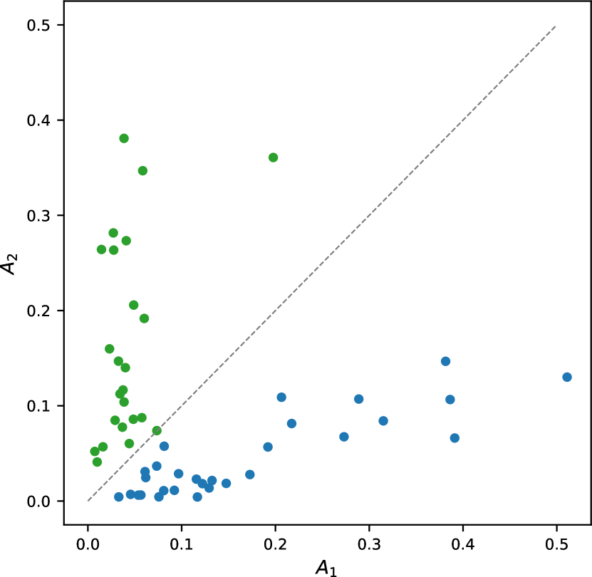
Figure 2: Amplitude $A_{2}$ vs $A_{1}$ for the folded lightcurves. Double peaked lightcurves (green dots) have $A_{2}>A_{1}$ while the single peaked folded lightcurves (blue dots) have $A_{2}<A_{1}$.

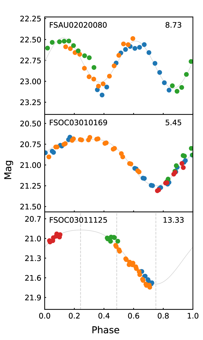
Figure 3: The upper and mid panels show double peaked and single peaked folded lightcurves, respectively. The lower panel shows single peaked folded lightcurve with insufficient coverage. Dashed lines indicate the minimum, maximum, and points where the fit lightcurve crosses the mean magnitude $\bar{m}$. This lightcurve is rejected because there are no points in the fourth section. Note that the object ID and derived rotation period are indicated on each plot. Different colors represent data points obtained from different nights. The gray lines are the fitting results.

Since observations were conducted near opposition, we are able to use the rates of motion along the Ecliptic longitude and latitude to distinguish different populations of moving objects (e.g. Yoshida & Terai, 2017). As shown in Figure 1, the observed moving objects can be classified as MBAs, Hildas, JTs, and Trans-Neptunian Objects (TNOs). Moreover, several Near Earth Asteroids (NEAs) and Centaurs are also evident. We used the objects corresponding to the orange points in Figure 1 as our sample of JTs for further rotation period analysis, and the JTs for which we found periods are indicated by the green dots. In total, 1241 JTs (hereinafter FOSSIL JTs) with detections in five or more epochs were chosen, including 63 previously known JTs. (Note that no rotation periods had been measured for these 63 objects.)

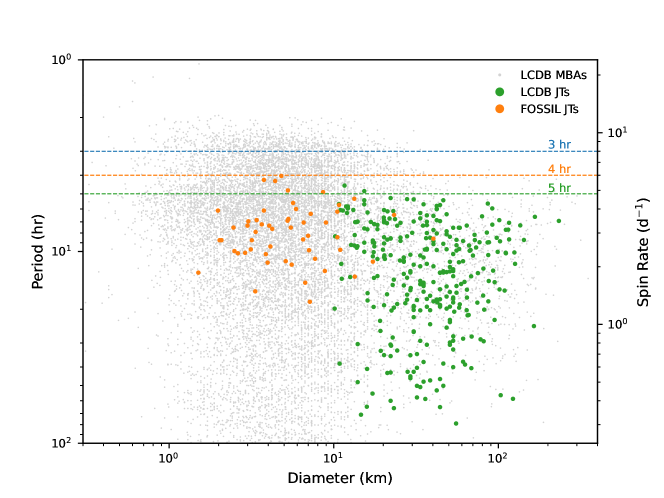
Figure 4: Rotation period and spin rate vs diameter for the FOSSIL JTs (orange dots). The same is shown for previously measured JTs (green dots) The green, orange, and blue dashed lines indicate rotation periods of 5, 4, and 3 hr, respectively. Note that only the objects with full and half derived rotation periods in our samples are used in this plot.

In order to estimate the diameters of the FOSSIL JTs, the distance to each object must be estimated. To that end, we assume a constant semi-major axis of $a=5.2$ au and eccentricity $e=0$ for each JT. Since the phase angles of FOSSIL JTs only have small changes during our observations, we simply estimate their absolute magnitudes using a fixed $G$ slope of 0.15 in the $H$–$G$ system (Bowell et al., 1989). Diameters were then estimated (Yoshida & Terai, 2017) as

$$\log D=0.2m_{\odot}+\log 2r-0.5\log p-0.2H,$$ (1)

where $m_{\odot}$ is the apparent magnitude of the Sun, $r$ is the heliocentric distance of Earth in the same unit as $D$, $p$ is the geometric albedo, and $H$ is the absolute magnitude of the JT in the observed band. We adopt $m_{\odot}=-27.04$ for the $r2$ band and $-26.34$ for the $g$ band (Willmer, 2018), and we set $p=0.05$ (Romanishin & Tegler, 2018) for both bands.

3 Rotation-Period Analysis

To measure rotation period, we attempted to follow the method of Harris et al. (1989) and performed a 2nd-order Fourier series fit to the lightcurves of FOSSIL JTs:

$$m_{j}=\bar{m}+\sum_{k=1}^{2}\left\{B_{k}\sin\left[\frac{2\pi k}{P}(t_{j}-t_{0})\right]\right.\\ \left.+C_{k}\cos\left[\frac{2\pi k}{P}(t_{j}-t_{0})\right]\right\},$$ (2)

To determine whether the algorithm gives a good fit to the lightcurve, we calculate the difference between the reduced $\chi^{2}$ of the best-fit period and that of a fit to the mean magnitude. We found that when the difference is $>$2, the fitting shows a convincing folded lightcurve.

Based on the assumption of ellipsoidal shapes for JTs, a folded lightcurve with two minima and two maxima is expected. However, the best-fit (i.e., the minimum reduced $\chi^{2}$) period of this algorithm returns two types of folded lightcurves: double peaked and single peaked. Two conditions can give rise to a single peaked lightcurve: first, when all of the data are contained in the same half of the phased double peaked lightcurve, and second, when the two halves of the double peaked lightcurve are very similar. To distinguish between the two cases, we look at the amplitudes of each phase $k$ of the Fourier series fit

$$A_{k}=(B_{k}^{2}+C_{k}^{2})^{\frac{1}{2}}.$$ (3)

For a double peaked lightcurve, the amplitude of the $k=2$ Fourier component is larger, with a smaller correction by the $k=1$ component. When a single peaked folded lightcurve is found, the opposite is true. We can then thus distinguish between the two cases by defining a folded lightcurve as double peaked when $A_{2}>A_{1}$ and single peaked when $A_{1}\geq A_{2}$. Figure 2 shows a plot of $A_{1}$ vs $A_{2}$ for the JTs where a good fit was found, and Figure 3 shows example double and single peaked folded lightcurves. Note that in most cases it is obvious if the fit lightcurve is single or double peaked, but there are some marginal cases when the amplitude is low, and this method also facilitates automation of the analysis.

When the best-fit period gives a single peaked lightcurve, the next best local minimum of the reduced $\chi^{2}$ vs $P$ curve with a longer period is selected as the preferred solution. However, this does not always work well when there is not sufficiently full coverage of the single peaked folded lightcurve. To eliminate such cases, we divide each single peak folded lightcurve into four sections bounded by the minimum, maximum, and the two points where the fit lightcurve crosses the mean magnitude $\bar{m}$ (see Figure 3). We require that there be at least two points in each section, otherwise we reject the lightcurve since we cannot be confident of the fit period. Finally, when using the second local minimum for the period, in some cases unrealistic fit parameters are returned (e.g. a lightcurve amplitude of 80 mag). In such cases, we have found that the fit period is always more than three times the fit period for the original single peaked folded lightcurve. We thus reject any fits where the new period is three times longer than that from the original fit.

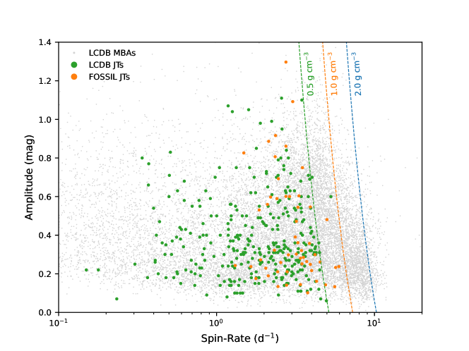
Figure 5: Spin rate vs amplitude of FOSSIL JTs (orange dots) and JTs (green dots) and MBAs (gray dots) found in the LCDB. The green, orange, and blue dashed lines are the rotation period limits for rubble-pile asteroids with bulk densities of 0.5, 1, and 2 g cm^-3, respectively, calculated from Equation 4.

From the lightcurves of the 1241 FOSSIL JTs, we obtained 40 double peaked folded lightcurves which passed our selection criteria. In addition, we found 13 single peaked folded lightcurves from which we were able to recalculate double peaked lightcurves which passed the cuts outlined above. The main reason for the low rate of successful period fitting is due to the fact that most of the detections are of fainter objects, and the lightcurves of these objects are therefore too noisy to obtain an accurate fit given the short span of our observations. In addition, due to the short time span of our observations at each block, our analysis is insensitive to longer period rotation curves.

Photometric data for these 53 lightcurves are presented in Table 2. Diameters, rotation periods, lightcurve amplitudes, and folded lightcurve fit parameters for each of these objects are shown in Table 3 in the appendix. The folded lightcurves of these objects are also shown in the appendix in Figures 6 and 7.

4 Results and Discussion

Figure 4 shows a plot of diameter vs rotation period for the FOSSIL JTs where full and half rotation periods are found. For comparison, the values for previously measured rotation periods for are also shown. The FOSSIL data set extends the range of diameters of JTs with measured rotation periods from $D\gtrsim 10$ km down to $D\gtrsim 1$ km for the first time. We note that there is a clear lack of long period detections in the FOSSIL data. This is due to biases against long periods in our survey arising from the short time span of observations at each block of pointings.

In the sample of smaller diameter JTs found by FOSSIL, five of them have rotation periods faster than the previously suggested 5-hr limit,

Assuming a rubble-pile structure for JTs, the minimum bulk density to withstand these spin rates can be calculated (Harris, 1996) using

$$P=3.3\left(\frac{1+\delta m}{\rho}\right)^{\frac{1}{2}},$$ (4)

where $P$ is the period in hr, $\rho$ is the bulk density in g cm^-3, and $\delta m$ is the lightcurve amplitude in mag. We estimate the lightcurve amplitude $\delta m$ as 95% of the difference between the brightest and fainted measurements for each object, given that the folded lightcurve fits sometimes significantly overestimate the amplitudes. Figure 5 shows a plot of spin rate vs lightcurve amplitude for both the FOSSIL JTs and previously measured JTs, along with limits on bulk density calculated from Equation 4. Given the rotation rates measured for the FOSSIL JTs, these objects need a bulk density of at least $\approx$0.9 g cm^-3, a value consistent with the measurements of $\sim 0.8-1.0$ g cm^-3 (Marchis et al., 2006; Mueller et al., 2010; Buie et al., 2015; Berthier et al., 2020) from the binary JT system, (617) Patroclus–Menoetius system and much higher than that derived from the 5-hr spin-rate limit (i.e., $\sim$0.5 g cm^-3 Ryan et al., 2017; Szabó et al., 2017, 2020; Kalup et al., 2021).

5 Summary and Conclusions

Using the Subaru/HSC, a wide-field high-cadence survey, part of which was to measure rotation periods of small JTs, was conducted in 2019 and 2020. From this survey, we report the detection of 1241 JTs, only 63 of which are found in the MPC database. We were able to obtain rotation periods for 53 of the 1241 JTs, the vast majority of which were measured on objects with diameters $D<10$ km, an order of magnitude smaller than previously accomplished. We found a number of objects with periods near 4 hr, significantly lower than the suggested limit of 5 hr. Under the assumption of a rubble-pile structure for JTs, a bulk density of $\approx$0.9 g cm^-3 is required to maintain their structure at that rotation period limit. This value is comparable to the measurements of $\sim 0.8-1.0$ g cm^-3 (Marchis et al., 2006; Mueller et al., 2010; Buie et al., 2015; Berthier et al., 2020) from the binary JT system, (617) Patroclus–Menoetius.

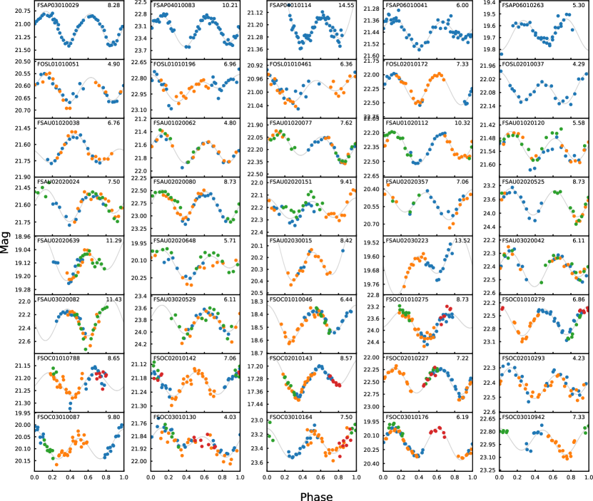
Figure 6: 40 folded lightcurves of JTs where a double peak fit was returned. The object ID and derived rotation period are indicated on each plot. Different colors represent data points obtained from different nights. The gray lines are the fitting results. Photometric errors are too small to be seen in the plots.

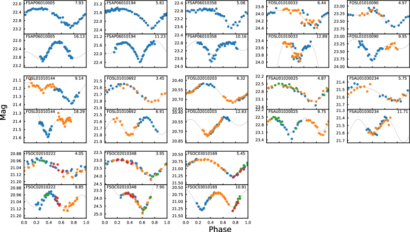
Figure 7: 13 folded lightcurves of JTs where a single peak fit as returned. The top plots in each frame show the results from the original single peak fits, and the bottom plots show the folded lightcurves when a double peaked period was found in a second round of fitting. The object ID and half period are indicated on each plot. Symbols are the same as in Figure 6. Photometric errors are too small to be seen in the plots.

Table 3: Physical parameters for FOSSIL JTs for which rotation periods were obtained.

JT ID	MPC Designation	Block	$H$ (mag)		$D$ (km)		$\sigma_{D}$ (km)		$P$ (hr)		$\sigma_{P}$ (hr)		$\delta m$ (mag)	$\bar{m}$ (mag)	$B_{1}$	$C_{1}$	$B_{2}$	$C_{2}$
FSAP03010029	(156294) 2001 WU66	19Apr	14.4	6.99	0.56	8.28	0.15	0.60	21.1	0.02	-0.02	0.12	0.25
FSAP04010083		19Apr	16.5	2.62	0.21	10.21	0.70	0.81	23.2	-0.05	0.03	-0.17	-0.30
FSAP04010114		19Apr	14.5	6.71	0.54	14.56	4.28	0.24	21.2	-0.03	-0.13	-0.09	-0.10
FSAP06010041		19Apr	14.7	5.90	0.48	6.00	0.23	0.22	21.4	-0.04	-0.00	0.05	-0.06
FSAP06010263	(24022) 1999 RA144	19Apr	13.0	13.3	1.1	5.30	0.21	0.26	19.7	0.02	-0.03	-0.11	-0.03
FOSL01010051	(523904) 1997 JF7	20May	13.9	8.62	0.70	4.898	0.049	0.14	20.6	-0.01	-0.00	0.02	0.05
FOSL01010196		20May	16.2	3.03	0.24	6.96	0.15	0.32	22.9	-0.04	0.06	-0.06	-0.05
FOSL01010461	2011 PQ10	20May	14.3	7.25	0.59	6.36	0.13	0.10	21.0	-0.01	0.02	-0.03	-0.01
FOSL02010172		20May	15.6	4.06	0.33	7.328	0.056	0.54	22.2	0.02	0.02	0.25	-0.09
FOSL02010037		20May	15.4	4.41	0.36	4.28	0.35	0.13	22.1	0.00	-0.03	0.04	-0.04
FSAU01020038		20Aug	15.0	5.31	0.43	6.761	0.048	0.29	21.7	0.07	-0.00	0.00	0.09
FSAU01020062		20Aug	15.0	5.27	0.43	4.800	0.024	0.48	21.7	-0.01	0.06	0.03	-0.19
FSAU01020077		20Aug	15.5	4.23	0.34	7.619	0.061	0.39	22.2	-0.01	-0.04	0.11	-0.08
FSAU01020112		20Aug	15.7	3.87	0.31	10.32	0.11	0.32	22.4	-0.00	0.03	-0.13	0.07
FSAU01020120		20Aug	14.8	5.67	0.46	5.581	0.033	0.16	21.5	-0.00	0.02	0.04	-0.04
FSAU02020024		20Aug	14.9	5.48	0.44	7.500	0.059	0.30	21.6	-0.03	-0.02	0.11	0.02
FSAU02020080		20Aug	16.1	3.18	0.26	8.727	0.080	0.60	22.8	-0.01	-0.04	0.27	0.02
FSAU02020151		20Aug	15.5	4.13	0.33	9.41	0.19	0.26	22.2	-0.01	0.01	0.05	-0.05
FSAU02020357	2015 CO51	20Aug	13.8	8.97	0.72	7.06	0.10	0.28	20.5	0.02	-0.03	-0.05	0.09
FSAU02020525		20Aug	17.0	2.08	0.17	8.727	0.080	0.86	23.7	-0.04	0.01	-0.30	0.23
FSAU02020639	(100624) 1997 TR28	20Aug	12.4	17.3	1.4	11.29	0.13	0.19	19.1	-0.02	-0.07	-0.09	0.01
FSAU02020648	(221909) 2008 QY14	20Aug	13.4	10.77	0.87	5.714	0.069	0.30	20.1	-0.06	-0.00	0.07	-0.05
FSAU02030015	(286571) 2002 CR207	20Aug	13.5	10.52	0.85	8.42	0.15	0.30	20.2	-0.03	-0.15	-0.11	-0.13
FSAU02030223	(257375) 2009 QZ47	20Aug	13.0	13.4	1.1	13.52	0.72	0.18	19.6	-0.09	0.02	0.09	-0.06
FSAU03020042		20Aug	15.7	3.76	0.30	6.115	0.079	0.25	22.4	0.02	-0.03	-0.10	-0.02
FSAU03020082		20Aug	15.6	3.97	0.32	11.43	0.28	0.56	22.3	0.08	0.01	0.17	0.18
FSAU03020529		20Aug	17.1	1.98	0.16	6.115	0.039	0.55	23.8	-0.05	0.01	0.18	0.10
FSOC01010046		20Oct	11.8	23.3	1.9	6.443	0.044	0.26	18.5	0.00	0.04	-0.08	0.07
FSOC01010275		20Oct	17.1	2.03	0.16	8.727	0.080	1.30	23.8	-0.16	-0.12	0.36	0.01
FSOC01010279		20Oct	15.9	3.40	0.27	6.857	0.049	0.75	22.6	0.04	-0.01	0.29	0.13
FSOC01010788	(396413) 2014 ED23	20Oct	14.5	6.52	0.53	8.65	0.23	0.14	21.2	0.00	0.01	0.01	0.04
FSOC02010142	(356253) 2009 UK77	20Oct	14.5	6.57	0.53	7.06	0.10	0.14	21.2	0.00	0.00	0.02	0.05
FSOC02010143	(14690) 2000 AR25	20Oct	10.6	40.3	3.3	8.571	0.077	0.21	17.3	-0.01	-0.05	-0.07	0.04
FSOC02010227		20Oct	15.8	3.65	0.30	7.218	0.055	0.60	22.5	-0.01	-0.01	0.19	-0.18
FSOC02010293		20Oct	15.7	3.77	0.30	4.229	0.037	0.23	22.4	0.02	0.02	-0.01	0.08
FSOC03010087		20Oct	13.4	10.96	0.89	9.80	0.10	0.13	20.1	0.02	0.00	-0.01	0.05
FSOC03010130		20Oct	15.2	4.81	0.39	4.034	0.017	0.24	21.9	-0.03	0.03	-0.02	0.06
FSOC03010164		20Oct	16.6	2.46	0.20	7.500	0.059	0.47	23.3	0.04	-0.04	0.03	-0.17
FSOC03010176	(263794) 2008 QQ37	20Oct	13.5	10.52	0.85	6.194	0.040	0.36	20.2	-0.01	-0.02	0.13	0.09
FSOC03010942		20Oct	16.2	2.99	0.24	7.33	0.16	0.36	22.9	0.01	0.03	0.13	-0.02
FSAP06010005		19Apr	16.0	3.34	0.27	16.13	1.81	0.83	22.7	0.21	0.14	-0.26	0.06
FSAP06010194	2012 VQ5	19Apr	15.0	5.11	0.41	11.23	0.70	0.89	21.7	0.06	-0.00	-0.22	-0.23
FSAP06010358		19Apr	16.3	2.90	0.23	10.2	1.1	0.92	23.0	-0.06	-0.07	0.22	0.17
FOSL01010033		20May	17.7	1.51	0.12	12.89	0.54	0.53	24.4	0.52	0.39	0.43	-0.16
FOSL01010090		20May	16.6	2.50	0.20	9.95	0.30	0.59	23.3	-0.15	-0.05	0.14	0.07
FOSL01010144		20May	14.3	7.16	0.58	18.29	0.99	0.24	21.0	0.01	0.33	-0.08	-0.14
FOSL01010692	2011 OR64	20May	15.0	5.25	0.42	6.91	0.15	0.25	21.7	0.00	-0.02	-0.08	-0.09
FOSL02010203	(457150) 2008 FD133	20May	13.9	8.84	0.71	12.63	0.34	0.27	20.6	-0.03	-0.06	0.08	0.02
FSAU01020025		20Aug	16.1	3.14	0.25	9.75	0.19	0.69	22.8	0.01	0.03	-0.09	0.27
FSAU01030234		20Aug	14.9	5.55	0.45	11.71	0.60	0.23	21.6	-0.06	-0.02	0.07	-0.10
FSOC02010222	2015 FP40	20Oct	14.3	7.08	0.57	9.84	0.10	0.21	21.0	-0.01	0.01	-0.02	-0.07
FSOC02010348		20Oct	16.0	3.35	0.27	7.90	0.13	1.09	22.7	-1.02	-0.43	-0.67	-0.04
FSOC03010169	(295699) 2008 TC173	20Oct	14.2	7.71	0.62	10.91	0.13	0.60	20.9	-0.01	-0.04	-0.28	-0.09

Note. — MPC designations are provided for previously known JTs.

References

- Berthier et al. (2020) Berthier, J., Descamps, P., Vachier, F., et al. 2020, Icarus, 352, 113990, doi: 10.1016/j.icarus.2020.113990
- Bosch et al. (2018) Bosch, J., Armstrong, R., Bickerton, S., et al. 2018, PASJ, 70, S5, doi: 10.1093/pasj/psx080
- Bowell et al. (1989) Bowell, E., Hapke, B., Domingue, D., et al. 1989, in Asteroids II, ed. R. P. Binzel, T. Gehrels, & M. S. Matthews, 524–556
- Buie et al. (2015) Buie, M. W., Olkin, C. B., Merline, W. J., et al. 2015, AJ, 149, 113, doi: 10.1088/0004-6256/149/3/113
- Chambers et al. (2017) Chambers, K. C., et al. 2017, VizieR Online Data Catalog, II/349
- Chang et al. (2016) Chang, C.-K., Lin, H.-W., Ip, W.-H., et al. 2016, ApJS, 227, 20, doi: 10.3847/0067-0049/227/2/20
- Chang et al. (2015) Chang, C.-K., Ip, W.-H., Lin, H.-W., et al. 2015, ApJS, 219, 27, doi: 10.1088/0067-0049/219/2/27
- Chang et al. (2019) Chang, C.-K., Lin, H.-W., Ip, W.-H., et al. 2019, ApJS, 241, 6, doi: 10.3847/1538-4365/ab01fe
- Chapman (1978) Chapman, C. R. 1978, in NASA Conference Publication, Vol. 2053, NASA Conference Publication, ed. D. Morrison & W. C. Wells, 145–160
- Davis et al. (1985) Davis, D. R., Chapman, C. R., Weidenschilling, S. J., & Greenberg, R. 1985, Icarus, 62, 30, doi: 10.1016/0019-1035(85)90170-8
- DeMeo & Carry (2013) DeMeo, F. E., & Carry, B. 2013, Icarus, 226, 723, doi: 10.1016/j.icarus.2013.06.027
- Duda & Hart (1972) Duda, R. O., & Hart, P. E. 1972, Commun. ACM, 15, 11, doi: 10.1145/361237.361242
- Emery et al. (2011) Emery, J. P., Burr, D. M., & Cruikshank, D. P. 2011, AJ, 141, 25, doi: 10.1088/0004-6256/141/1/25
- Fernandez & Ip (1984) Fernandez, J. A., & Ip, W. H. 1984, Icarus, 58, 109, doi: 10.1016/0019-1035(84)90101-5
- Fleming & Hamilton (2000) Fleming, H. J., & Hamilton, D. P. 2000, Icarus, 148, 479, doi: 10.1006/icar.2000.6523
- Fraser et al. (2016a) Fraser, W., Alexandersen, M., Schwamb, M. E., et al. 2016a, AJ, 151, 158, doi: 10.3847/0004-6256/151/6/158
- Fraser & Brown (2018) Fraser, W. C., & Brown, M. E. 2018, AJ, 156, 23, doi: 10.3847/1538-3881/aac213
- Fraser et al. (2016b) Fraser, W. C., Alexandersen, M., Schwamb, M. E., et al. 2016b, TRIPPy: Python-based Trailed Source Photometry. http://ascl.net/1605.010
- Furusawa et al. (2018) Furusawa, H., Koike, M., Takata, T., et al. 2018, PASJ, 70, S3, doi: 10.1093/pasj/psx079
- Grundy et al. (2019) Grundy, W. M., Noll, K. S., Buie, M. W., et al. 2019, Icarus, 334, 30, doi: 10.1016/j.icarus.2018.12.037
- Harris (1996) Harris, A. W. 1996, in Lunar and Planetary Science Conference, Vol. 27, Lunar and Planetary Science Conference, 493
- Harris et al. (1989) Harris, A. W., Young, J. W., Bowell, E., et al. 1989, Icarus, 77, 171, doi: 10.1016/0019-1035(89)90015-8
- Hirabayashi (2015) Hirabayashi, M. 2015, MNRAS, 454, 2249, doi: 10.1093/mnras/stv2017
- Holsapple (2007) Holsapple, K. A. 2007, Icarus, 187, 500, doi: 10.1016/j.icarus.2006.08.012
- Hough (1959) Hough, P. V. C. 1959, Conf. Proc. C, 590914, 554
- Hu et al. (2021) Hu, S., Richardson, D. C., Zhang, Y., & Ji, J. 2021, MNRAS, doi: 10.1093/mnras/stab412
- Kalup et al. (2021) Kalup, C. E., Molnár, L., Kiss, C., et al. 2021, ApJS, 254, 7, doi: 10.3847/1538-4365/abe76a
- Kawanomoto et al. (2018) Kawanomoto, S., Uraguchi, F., Komiyama, Y., et al. 2018, PASJ, 70, 66, doi: 10.1093/pasj/psy056
- Komiyama et al. (2018) Komiyama, Y., Obuchi, Y., Nakaya, H., et al. 2018, PASJ, 70, S2, doi: 10.1093/pasj/psx069
- Lykawka & Horner (2010) Lykawka, P. S., & Horner, J. 2010, MNRAS, 405, 1375, doi: 10.1111/j.1365-2966.2010.16538.x
- Malhotra (1995) Malhotra, R. 1995, AJ, 110, 420, doi: 10.1086/117532
- Mann et al. (2007) Mann, R. K., Jewitt, D., & Lacerda, P. 2007, AJ, 134, 1133, doi: 10.1086/520328
- Marchis et al. (2006) Marchis, F., Hestroffer, D., Descamps, P., et al. 2006, Nature, 439, 565, doi: 10.1038/nature04350
- Marzari & Scholl (1998) Marzari, F., & Scholl, H. 1998, Icarus, 131, 41, doi: 10.1006/icar.1997.5841
- Masiero et al. (2009) Masiero, J., Jedicke, R., Ďurech, J., et al. 2009, Icarus, 204, 145, doi: 10.1016/j.icarus.2009.06.012
- Miyazaki et al. (2018) Miyazaki, S., Komiyama, Y., Kawanomoto, S., et al. 2018, PASJ, 70, S1, doi: 10.1093/pasj/psx063
- Morbidelli et al. (2005) Morbidelli, A., Levison, H. F., Tsiganis, K., & Gomes, R. 2005, Nature, 435, 462, doi: 10.1038/nature03540
- Mueller et al. (2010) Mueller, M., Marchis, F., Emery, J. P., et al. 2010, Icarus, 205, 505, doi: 10.1016/j.icarus.2009.07.043
- Nesvorný et al. (2020) Nesvorný, D., Vokrouhlický, D., Bottke, W. F., Levison, H. F., & Grundy, W. M. 2020, ApJ, 893, L16, doi: 10.3847/2041-8213/ab8311
- Nesvorný et al. (2013) Nesvorný, D., Vokrouhlický, D., & Morbidelli, A. 2013, ApJ, 768, 45, doi: 10.1088/0004-637X/768/1/45
- Polishook et al. (2012) Polishook, D., Ofek, E. O., Waszczak, A., et al. 2012, MNRAS, 421, 2094, doi: 10.1111/j.1365-2966.2012.20462.x
- Romanishin & Tegler (2018) Romanishin, W., & Tegler, S. C. 2018, AJ, 156, 19, doi: 10.3847/1538-3881/aac210
- Rozitis & Green (2013) Rozitis, B., & Green, S. F. 2013, MNRAS, 430, 1376, doi: 10.1093/mnras/sts723
- Rubincam (2000) Rubincam, D. P. 2000, Icarus, 148, 2, doi: 10.1006/icar.2000.6485
- Ryan et al. (2017) Ryan, E. L., Sharkey, B. N. L., & Woodward, C. E. 2017, AJ, 153, 116, doi: 10.3847/1538-3881/153/3/116
- Sonnett et al. (2015) Sonnett, S., Mainzer, A., Grav, T., Masiero, J., & Bauer, J. 2015, ApJ, 799, 191, doi: 10.1088/0004-637X/799/2/191
- Szabó et al. (2017) Szabó, G. M., Pál, A., Kiss, C., et al. 2017, A&A, 599, A44, doi: 10.1051/0004-6361/201629401
- Szabó et al. (2020) Szabó, G. M., Kiss, C., Szakáts, R., et al. 2020, ApJS, 247, 34, doi: 10.3847/1538-4365/ab6b23
- Warner et al. (2009) Warner, B. D., Harris, A. W., & Pravec, P. 2009, Icarus, 202, 134, doi: 10.1016/j.icarus.2009.02.003
- Weissman (1986) Weissman, P. R. 1986, Nature, 320, 242, doi: 10.1038/320242a0
- Willmer (2018) Willmer, C. N. A. 2018, ApJS, 236, 47, doi: 10.3847/1538-4365/aabfdf
- Wong & Brown (2015) Wong, I., & Brown, M. E. 2015, AJ, 150, 174, doi: 10.1088/0004-6256/150/6/174
- Wong et al. (2014) Wong, I., Brown, M. E., & Emery, J. P. 2014, AJ, 148, 112, doi: 10.1088/0004-6256/148/6/112
- Yoshida & Terai (2017) Yoshida, F., & Terai, T. 2017, AJ, 154, 71, doi: 10.3847/1538-3881/aa7d03