Time Series Estimation of the Dynamic Effects of Disaster-Type Shocks

Abstract

This paper provides three results for SVARs under the assumption that the primitive shocks are mutually independent. First, a framework is proposed to accommodate a disaster-type variable with infinite variance into a SVAR. We show that the least squares estimates of the SVAR are consistent but have non-standard asymptotics. Second, the disaster shock is identified as the component with the largest kurtosis and whose impact effect is negative. An estimator that is robust to infinite variance is used to recover the mutually independent components. Third, an independence test on the residuals pre-whitened by the Choleski decomposition is proposed to test the restrictions imposed on a SVAR. The test can be applied whether the data have fat or thin tails, and to over as well as exactly identified models. Three applications are considered. In the first, the independence test is used to shed light on the conflicting evidence regarding the role of uncertainty in economic fluctuations. In the second, disaster shocks are shown to have short term economic impact arising mostly from feedback dynamics. The third uses the framework to study the dynamic effects of economic shocks post-covid.

JEL Classification: C21, C22
Keywords: Heavy-tails, independent component analysis, distance covariance

1 Introduction

The novel coronavirus (covid-19) outbreak has drawn attention to the modeling of rare events such as pandemics and natural disasters. How do we estimate the dynamic effects of disaster type shocks on economic variables? How do we estimate the dynamic effects of economic shocks when the data are contaminated by rare events that do not have economic origins? Should measures of disasters be modeled as exogenous? A difficulty in predicting the occurrence of disasters and designing polices to mitigate their impact is that there are few such data points even over a long span. After all, the CDC has only documented four influenza pandemics in the U.S. with deaths in excess of 100,000 over a 120 year period starting in 1900. For natural disasters, the 12,000 deaths from the Galveston hurricane of 1900 remains a record, with the 1200 deaths from Katrina coming in a distant second in terms of casualties. Worldwide, only seven earthquakes since 1500 were larger than 9 in magnitude, and September 11 was the only terror attack on U.S. soil with more than 300 deaths, let alone 3000. Nonetheless, when a rare disaster strikes, it strikes in a ferocious manner as covid-19 reminds us. Though these events have been intensely studied on a case by case basis, it is also of interest to study these events over a long time span. We apply standard time series methodology to analyze the dynamic effects of rare events by modeling these events as being driven by heavy-tailed shocks.

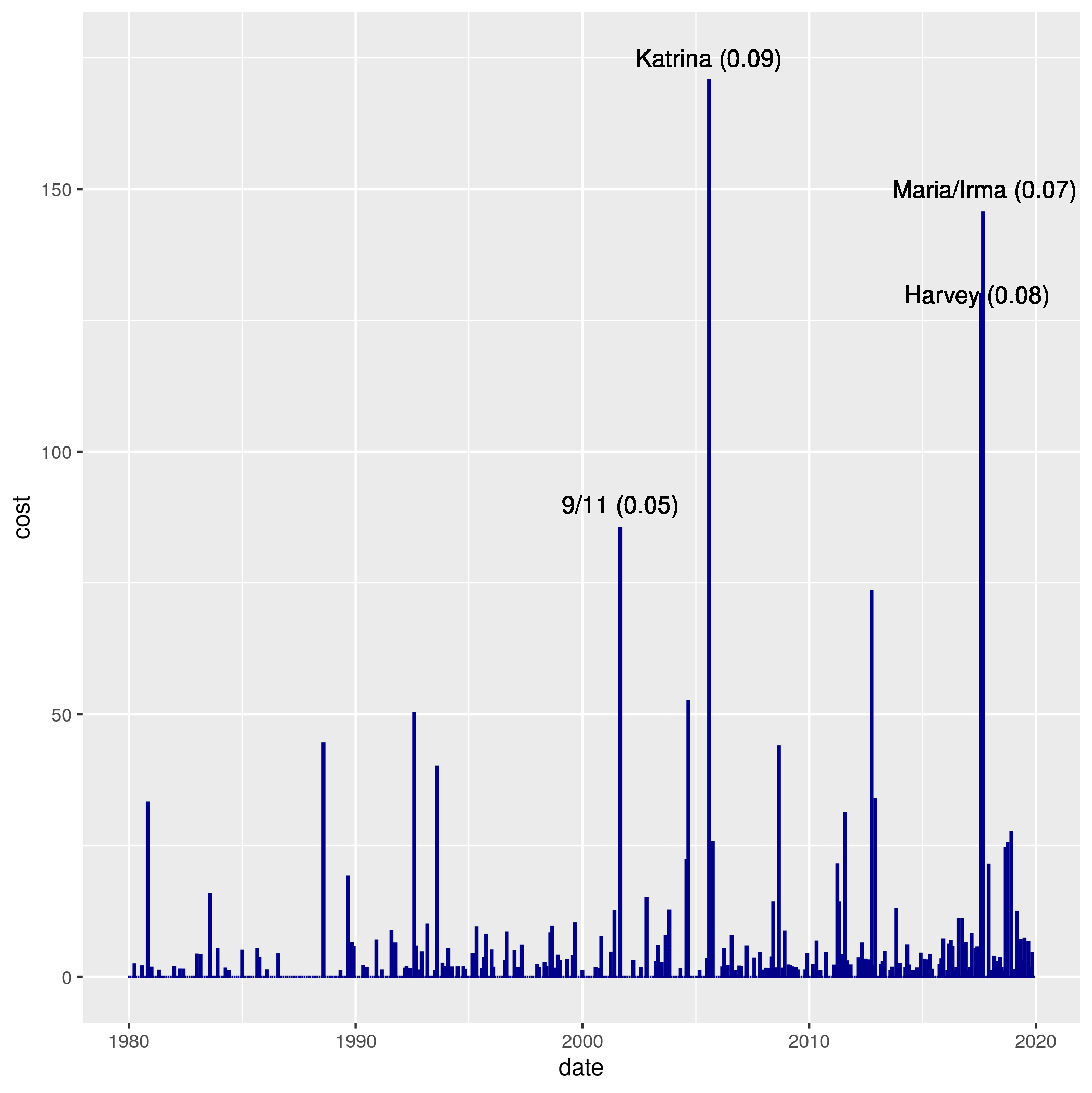
Figure 1: Real Cost of Disasters: 1980:1-2019:12

To fix ideas, consider Figure 1 which plots the real cost of 258 natural disasters over the period 1980:1-2019:12, augmented to include 9/11. The series is dominated by a few events with Hurricane Katrina in August 2005 being the largest, accounting for 9.2% of total cost. This is followed by the four weeks in the summer of 2017 when Hurricane Harvey contributed 7% in August, while Hurricanes Irma and Maria in September created a combined cost of 8%. These are followed by 9/11 in 2001 and superstorm Sandy in October 2012, each contributing to about 5% of total costs. Another measure of the cost of disasters is the number of lives lost. This series, while not plotted to conserve space, has spikes that are even more extreme. Over the same time period, 49% of disaster-related deaths can be attributed to Hurricanes Maria/Irma, 9/11, and Hurricane Katrina, with the heat wave of 1980 coming in fourth. Both series have features of a heavy-tailed process, and we will subsequently use sample kurtosis as evidence of tail heaviness.

Heavy-tailed data pack a lot of information in a few observations. Because of its large variability, the dynamic effects of disaster shocks should in principle be consistently estimable. Indeed, if all variables in a multivariate system have heavy tails, we show below that the least squares estimator will converge at a fast rate of $(\frac{T}{\ln T})^{1/\alpha}$ where $\alpha$ is the index of the heavy-tailed shock and $T$ is the sample size. Though the distribution theory is a bit nonstandard, the regression framework is the same as the standard case when all variables have light tails. But while many macroeconomic time series have excess kurtosis, they do not fit the characterization of heavy tails. For example, unemployment and industrial production have kurtosis of less than 10, while the disaster series shown in Figure 1 has kurtosis in excess of 70, and the estimated tail index of approximately one suggests a distribution with infinite variance and possibly infinite mean. Beare and Toda (2020) analyzed covid-19 cases across US counties and finds that the right tail of the distribution has a Pareto exponent close to one. This motivates a new multivariate framework in which finite and infinite variance shocks co-exist in such a way that the economic variables can be affected by heavy-tailed shocks but not dominated by them.

Our point of departure is that the $n$ primitive shocks $u=(u_{1},\ldots,u_{n})$ are assumed to be mutually independent, a condition stronger than the commonly used assumption of mutual orthogonality that is no longer meaningful when one of the shocks has infinite variance. We develop a HL (‘heavy-light’) framework in which the coefficient estimates on the infinite variance regressors are consistent at a rate of $T^{1/\alpha}$, still faster than the usual rate of $\sqrt{T}$. We then show that the disaster shock series can be identified by the magnitude of its kurtosis and the sign of its impact effect. For estimation, we perform an independent components analysis (ICA) based on distance covariance of the pre-whitened data, an approach first suggested in Matteson and Tsay (2017) for finite variance data. Davis and Fernandes (2022) recently showed that the procedure remains valid when a shock has infinite variance provided its mean is finite.

Prewhitening by singular value decomposition is often used to remove correlations prior to ICA estimation to focus on the higher order signals. For SVAR applications, prewhitening by Choleski decomposition is more natural since it is already used to identify mutually uncorrelated shocks with a recursive structure. We show that even though the variance of the shocks may not exist, Choleski decomposition of the sample covariance remains valid. Furthermore, we show that ICA will still recover the shocks in spite of sampling uncertainty in the VAR residuals. To assess the restrictions imposed on the SVAR, we apply a permutation-based procedure to the distance covariance statistic as a test for independence that is robust to infinite variance data. It complements other SVAR specification tests made possible by the independence assumption, as discussed below.

The rest of the paper is structured as follows. Section 2 summarizes the key properties of heavy-tailed linear processes and discusses the implications for VAR estimation. Section 3 presents the HL framework. Consistency and limiting behavior of the least squares estimator for parameters in a VAR are shown. Identification, estimation via distance covariance, and implementation of an independence test are then discussed. Section 4 uses simulations and three applications to assess the properties of the proposed procedure. The appendix contains background material on distance covariance as well as proofs of the main results in Section 3.

2 Heavy-Tailed Linear Processes

Disaster events are rare and heavy tails can be a useful characterization of their probabilistic structure. Well known heavy-tailed distributions include the Student-$t$, $F$, Fréchet, as well as infinite variance stable and Pareto distributions.

Let $F(x)=P(Z\leq x)$ for $x\in\mathbb{R}$ be the distribution of an IID sequence of random variables $\{Z_{t},t=0,\pm 1,\pm 2,\ldots\}$. Then $F$ has Pareto-like tails with tail index $\alpha>0$ if

$$x^{\alpha}\mathbb{P}(|Z|>x)\rightarrow C,\quad x\rightarrow\infty\,,$$ (1)

where $C$ is a finite and positive constant and $\frac{\mathbb{P}(Z>x)}{\mathbb{P}(|Z|>x)}\rightarrow p\in[0,1]$ as $x\rightarrow\infty$. Examples include the Cauchy and Pareto distributions. The Gaussian distribution has ‘thin’ tails that decay faster than an exponential and is not included in this class. The results that follow can be extended to a more general condition on $F$ called regular variation in which (1) is replaced by

$$\frac{\mathbb{P}(|Z|>sx)}{\mathbb{P}(|Z|>s)}\rightarrow x^{-\alpha},\quad s\rightarrow\infty\,.$$

The normalizing constants in such an extension become less explicit so we stick to the Pareto-like tail assumption for tractability.

Let $d_{1T}=\inf\{x:\mathbb{P}(|Z_{1}|>x)\leq\frac{1}{T}\}$ be the $(1-\frac{1}{T})$-th quantile of $F$ and $d_{2T}=\text{inf}\{x:\mathbb{P}(|Z_{0}Z_{1}|>x)\leq T^{-1}\}$ be the corresponding quantile for the joint distribution of the product $Z_{0}Z_{1}$. Distributions with Pareto-like tails have $d_{1T}=T^{1/\alpha}C^{1/\alpha}$. Since $1-F(d_{1T})=1/T$ for continuous $F$, (1) implies

$$T\mathbb{P}(|Z_{t}|>d_{1T}x)\rightarrow x^{-\alpha},\quad\mbox{as $T\rightarrow\infty$\,,}$$ (2)

for all $x>0$. Similarly $T\mathbb{P}(|Z_{0}Z_{1}|>d_{2T}x)\rightarrow x^{-\alpha}$ (see Davis and Resnick (1986)). The population moments of $Z_{t}$ satisfying (1) are only defined up to order $\alpha$ since

$$\begin{cases}\mathbb{E}|Z_{t}|^{\delta}=\infty\quad\delta\geq\alpha,\\ \mathbb{E}|Z_{t}|^{\delta}<\infty\quad\delta<\alpha.\end{cases}$$

It is possible for the population variance to exist but the population kurtosis to be undefined. But even if the population moments do not exist, the sample moments can still have well defined limits. If $Z_{t}$ has a Pareto-like tails with index $\alpha\in(1,2)$, $Z_{t}^{2}$ also has Pareto-like tails with index $\alpha/2$, and it holds that

$$\begin{pmatrix}[r]d_{1T}^{-1}\sum_{t=1}^{T}(Z_{t}-EZ),&d_{1T}^{-2}\sum_{t=1}^{T}Z_{t}^{2},&d_{2T}^{-1}\sum_{t=1}^{T}(Z_{t}-\bar{Z})(Z_{t-h}-\bar{Z})\end{pmatrix}\smash{\mathop{\longrightarrow}\limits^{d}}\begin{pmatrix}S_{\alpha},&S_{\alpha/2,0},&S_{\alpha,h}\end{pmatrix}$$ (3)

where $\bar{Z}=\frac{1}{T}\sum_{t=1}^{T}Z_{t}$ is the sample mean, and for $h>0$, $S_{\alpha},S_{\alpha/2,0},S_{\alpha,h}$ are stable random variables with exponents, $\alpha,\alpha/2$, and $\alpha$ respectively. Their joint distributions can be found in Davis and Resnick (1986).

To gain a sense of the tail properties of the data under investigation, we will make use of the fact that if $Z_{t}$ is an IID Pareto sequence with tail index $\alpha=1$, then the sample kurtosis $\kappa_{4}$ has the property (see Cohen, Davis, and Samorodnitsky (2020)) that

$$\frac{1}{T}\kappa_{4}=\frac{\sum_{t=1}^{T}Z_{t}^{4}}{(\sum_{t=1}^{T}Z_{t}^{2})^{2}}\smash{\mathop{\longrightarrow}\limits^{d}}\frac{S_{\alpha/4}}{S_{\alpha/2}^{2}}.$$ (4)

The limit of kurtosis, scaled by the sample size, is a random variable between zero and one so the maximum kurtosis that can be observed asymptotically is $T$. Tabulating the distribution for $T=500$ and $T=1000$ with $\alpha=1$, we see that the quantiles roughly double with $T$. Based on simulations, the values of these quantiles are an upper bound for $\alpha\in(1,2)$.

$T$	1%	2.5%	5%	10%	50%	90%	95%	97.5%	99%
500	37.9	47.55	58.8	77.9	225.9	477.5	494/5	498.7	499.7
1000	76.8	95.4	119.0	151.7	445.6	952.8	987.4	996.8	999.4

As a point of reference, the disaster series shown in Figure 1 has $T=480$ and kurtosis of around 70, which is in the lower 10-th percentile. The number of deaths series mentioned in the Introduction has kurtosis of 147 and is in the 30-th percentile. In contrast, the kurtosis a typical of macro economic time series is under 10, hence the theory for heavy tails would be inappropriate. A multivariate system of time series with different tail properties thus necessitates a different setup.

There is a large literature on robust and quantile estimation of the parameters in a linear model to guard against extreme values which explicitly down-weights outliers. Blattberg and Sargent (1971) and Kadiyala (1972) show that the least squares estimator is unbiased when the error in the regression model is drawn from a general symmetric stable Paretian distribution, but it is not the best linear unbiased estimator. In the Cauchy case when $\alpha=1$, the best linear unbiased estimator is $y_{\tau}/x_{\tau}$ where $x_{\tau}=\max_{j}X_{j}$. A different viewpoint, also the one taken in this paper, is that the extreme values are of interest. Under this assumption and fixed regressors, Mikosch and de Vries (2013) provide a finite sample analysis of the tail probabilities of the single equation CAPM estimates to understand why they vary significantly across reported studies. We are interested in estimating dynamic causal effects in a multivariate setting when the regressors are stochastic, and one of the primitive shocks has heavy tails.

2.1 Implications for VAR Estimation

Consider $n$ mean zero variables $Y_{t}=(Y_{t1},\ldots,Y_{tn})^{\prime}$ represented by a VAR(p):

$$Y_{t} = A_{1}Y_{t-1}+\ldots+A_{p}Y_{t-p}+e_{t},$$

where $A(z)=I_{n}-A_{1}z-\ldots-A_{p}z^{p}$ is the matrix-valued AR polynomial. Provided that det$A(z)\neq 0$ for all $z\in\mathbb{C}$ such that $|z|\leq 1$, $A(z)^{-1}$ exists, the moving-average representation of the model is $Y_{t}=\Phi(L)e_{t}$ where $L$ is the lag operator, and $\Phi(L)=A(L)^{-1}$ with $\Phi_{0}=I_{n}$.

The standard OLS estimator $\hat{A}$ of $A$ is characterized by (see (26) and (27))

$$\hat{A}-A = \bigg{(}\sum_{t=1}^{T}e_{t}Y_{t-1}^{\prime}\bigg{)}\bigg{(}\sum_{t=1}^{T}Y_{t-1}Y_{t-1}^{\prime}\bigg{)}^{-1}.$$

These errors $e_{t}$ are mapped to a $n\times 1$ vector of primitive shocks $u_{t}=(u_{t1},\ldots,u_{tn})^{\prime}$ via a (time invariant) matrix $B$:

$$e_{t}=Bu_{t}\,,$$

where $u_{t}$ is usually assumed to be mean zero, mutually and serially uncorrelated and with $\Sigma_{u}=\mathbb{E}[u_{t}u_{t}^{\prime}]$ being a diagonal matrix. See, for example, Stock and Watson (2015) and Kilian and Lutkepohl (2017). The reduced form errors $e_{t}$ are usually assumed to have ‘light tails’ which is possible only if $u_{t}$ has light tails. A model that satisfies these standard assumptions will be referred to as the LL (light-light) hereafter. Under regularity conditions for least squares estimation, $\hat{A}$ is $\sqrt{T}$ consistent and asymptotically normal.

The modeling issues that arise when one of the primitive shocks in a SVAR has infinite variance are best understood in the $p=1$ and $n=2$ case. Consider first a HH (heavy-heavy) model in which both shocks have heavy tails.

Lemma 1

Let $\{Z_{t}\}$ be an IID sequence of random variables with Pareto-like tails (i.e., equation (1)) with index $\alpha\in(0,2)$ and $EZ_{t}=0$ if $\alpha>1$. Let

$$d_{1T}=T^{1/\alpha},\quad\quad d_{2T}=(T\log T)^{1/\alpha}.$$

If the sequence of constants $\{\psi_{j}\}$ are such that $\sum_{j=-\infty}^{\infty}|\psi_{j}|^{\delta}<\infty$ for some $\delta\in(0,\alpha)\cup[0,1]$, then

• the process $X_{t}=\sum_{j=-\infty}^{\infty}\psi_{j}Z_{t-j}$ exists with probability one and is strictly stationary.

• Let $\hat{\rho}(h)=\sum_{t=1}^{T-h}X_{t}X_{t-h}/\sum_{t=1}^{T}X_{t}^{2}$ be the sample autocorrelation at lag $h>0$ and suppose that $\sum_{j=-\infty}^{\infty}|j|\;|\psi_{j}|^{\delta}<\infty$ for some $\delta\in(0,\alpha)\cup[0,1]$. Then for $\alpha\neq 1$,

  $$(d_{1T}^{-2}\sum_{t=1}^{T}X_{t}^{2},\;d_{2T}^{-1}\sum_{t=1}^{T-h}X_{t}X_{t-h}) \smash{\mathop{\longrightarrow}\limits^{d}} (S_{\alpha/2,0},S_{\alpha,h})$$

  $$\bigg{(}\frac{T}{\log T}\bigg{)}^{1/\alpha}(\hat{\rho}(h)-\rho(h)) = \frac{S_{\alpha,h}}{S_{\alpha/2,0}}$$

  where $(S_{\alpha/2,0}$, $S_{\alpha,h}$) are independent stable random variables with indices $\alpha/2$ and $\alpha$, respectively. If $\alpha>1$, then the latter convergence also holds if $EZ_{t}\neq 0$ provided $\hat{\rho}(h)$ is replaced by its mean-corrected version, $\widetilde{\rho}(h)=\sum_{t=1}^{T-h}(X_{t}-{\bar{X}})(X_{t-h}-{\bar{X}})/\sum_{t=1}^{T}(X_{t}-{\bar{X}})^{2}$.

• $d_{2T}^{-1}\sum_{t=1}^{T}X_{t-1}Z_{t}\smash{\mathop{\longrightarrow}\limits^{d}}S_{\alpha}$, where $S_{\alpha}$ is a stable random variable with index $\alpha$.

By restricting attention to $0<\alpha<2$, we only consider processes with infinite variance. Even though $X_{t}$ is not covariance stationary (since $\mathbb{E}|X_{t}|^{2}=\infty$), part (i) states that the process $X_{t}$ exists and is strictly stationary. The stated results for the sample covariance and sample autocorrelation are due to Davis and Resnick (1986, Theorem 3.3) and also hold when $X_{t}$ is centered for $\alpha\in(1,2)$. Note that the convergence of $\hat{\rho}(h)$ is faster than the $\sqrt{T}$ rate obtained for finite innovation variance.

For VAR estimation, Lemma 1 can be used to show that

$$d_{2T}^{-1}\sum_{t=1}^{T}Bu_{t}Y_{t-1}^{\prime} = \sum_{h=0}^{\infty}B\bigg{(}(T\log T)^{-1/\alpha}\sum_{t=1}^{T}u_{t}u_{t-1-h}\bigg{)}\Psi_{h}^{\prime}\smash{\mathop{\longrightarrow}\limits^{d}}\sum_{h=0}^{\infty}BS_{uu,h}\Psi_{h}^{\prime}=:S_{Ye}$$

$$d_{1T}^{-2}\sum_{t=1}^{T}Y_{t-1}Y_{t-1}^{\prime} = \sum_{h=0}^{\infty}\Psi_{h}\bigg{(}T^{-2/\alpha}\sum_{t=1}^{T}u_{t}u_{t}^{\prime}\bigg{)}\Psi_{h}^{\prime}\smash{\mathop{\longrightarrow}\limits^{d}}\sum_{h=0}^{\infty}\Psi_{h}S_{uu,0}\Psi_{h}^{\prime}=:S_{YY}.$$

It then follows from continuous mapping that the least squares estimator is super consistent:

$$\bigg{(}\frac{T}{\log T}\bigg{)}^{1/\alpha}(\hat{A}-A) \smash{\mathop{\longrightarrow}\limits^{d}} S_{Ye}S_{YY}^{-1}.$$

Though the analysis is straightforward, this setup is unappealing for macroeconomic data because if $u_{t1}$ and $u_{t2}$ both have infinite variance, $Y_{t1}$ and $Y_{t2}$ must also have infinite variance. But a typical economic time series does not resemble the series shown in Figure 1. Not only is the disaster series much less persistent, its kurtosis (over 70) is an order of magnitude larger than for variables like output growth, inflation, and interest rates.

3 A VAR with Heavy and Light Tailed Shocks

Our goal is a model in which (i) a heavy tailed shock $u_{t1}$ co-exists with light tailed shocks $u_{ti},\,i=2,\ldots,n$, and (ii) $Y_{ti}$ is influenced by the current and past values of $u_{t1}$ but not dominated by them in a sense to be made precise. We consider the HL (heavy-light) model derived from the SVAR$(p)$

$$Y_{t} = A_{1}Y_{t-1}+\ldots+A_{p}Y_{t-p}+Bu_{t},$$ (5)

where for each $h=1,\ldots,p$, $A_{h}$ is a $n\times n$ matrix with $(i,j)$-th entry denoted $[A_{ij}^{(h)}]$, the coefficient of variable $j$ at lag $h$ in equation $i$. The entries $[B_{ij}]$ of the $n\times n$ matrix $B$ are similarly defined.

Assumption HL

• The sequence of $n$-dimension random vectors $\{u_{t}\}$ is iid and the components, $u_{ti}\,,i=1,\ldots,n$ are also independent. The $u_{t1}$ will have Pareto-like tails with index $1<\alpha<2$ and $\mathbb{E}[u_{t1}]=0$, while the remaining shocks $u_{ti}\,,i=2\ldots,n$ will have thin tails with mean zero and variance 1.

• The coefficient matrices $A_{h}$ for $h=1,\ldots,p$ and the matrix $B$ will satisfy the following conditions.

  $$A_{i1,T}^{(h)}=a_{i1}^{(h)}/T^{\theta}\,,~{}~{}i=2,\ldots,n,$$ (6)

  $$B_{i1,T}=b_{i1}/T^{\theta}\,,~{}~{}i=2,\ldots,n,$$ (7)

  with

  $$\theta=\frac{1}{\alpha}-\frac{1}{2}.$$ (8)

The primitive shocks $u_{ti}$ are assumed to be independent across $i$ and $t$ but does not preclude time varying second moments, though it is stronger than mutual orthogonality of $u_{t}$ typically assumed in SVAR modeling. Assumption HL (i) restricts attention to processes with tail index $1<\alpha<2$ and thus excludes Cauchy shocks. The assumption that the thin tailed shocks $u_{ti}\,,i=2,\ldots n$ have unit variance is without loss of generality, but it is important that their variances are finite. Since the variations of $u_{t1}$ will dominate those of $u_{ti}\,,i\geq 2$ when both are present, $Y_{t1}$ will have heavy tails and exhibit the large spikes originating from $u_{t1}$.

Assumption HL(ii) is motivated by the fact that $Y_{ti}$ cannot have finite variance unless $B_{i1}=0$ and $A_{i1}^{(h)}=0$ for all $h$. But the dynamic effects of $u_{t1}$ on $Y_{t+h,i}$ would then be zero at all lags by assumption, rendering the empirical exercise meaningless. Thus, the $Y_{ti}$ equation is modified to dampen the influence of $u_{t1}$ on $Y_{ti}$ at rate $\theta$ given in (8), so that $T^{-1/2}\sum_{t=1}^{T}u_{t1}/T^{\theta}=T^{-1/\alpha}\sum_{t=1}^{T}u_{t1}$ has a limit. Localizing $A_{i1,T}^{(h)}$ and $B_{i1,T}$ to zero is an asymptotic device to obtain this limit, but note that $A^{h}_{i1,T}$ and $B_{i1,T}$ are not time varying. Under assumption HL(ii), $Y_{t,T}$ is a triangular array that depends on $T$. To simplify notation, the explicit dependence on $T$ is suppressed.

A heavy-tailed linear time series must have a heavy-tailed shock as its primary source of variation, but it need not be exogenous. In our model, exogeneity would require that $A_{1j}=B_{1j}=0,\,j=2,\ldots,n$, in which case, any feedback from $Y_{ti}$, $i\geq 2$ to $Y_{t1}$ would be disabled. But such a model would not shed light on how macroeconomic outcomes might mitigate or amplify the effects of disasters. Assumption HL allows $A^{(h)}_{1j}$ and $B_{1j},\,j=2,\ldots n$ to be free parameters to be estimated.

Specializing to the $n=2$ and $p=1$ case with $Eu_{t1}^{2}=\infty$ and $Eu_{t2}^{2}<\infty$ we show in the Appendix that the following holds under Assumption HL

$$\frac{1}{\sqrt{T}}\sum_{t=1}^{T}Y_{t2} = \smash{\mathop{\longrightarrow}\limits^{d}}S^{*}_{Y,2}$$

$$\frac{1}{T}\sum_{t=1}^{T}Y_{t2}^{2} = \smash{\mathop{\longrightarrow}\limits^{d}}S^{*}_{YY,22},$$

where the limits have a stable distribution with index $\alpha$ and $\alpha/2$, respectively. Thus the sample first and second moments of $Y_{t2}$ have (random and possibly constant) limits even though one of its shocks has infinite variance. The implications for least squares estimation of the HL model can be summarized as follows.

Proposition 1

Suppose that the data are generated by (5), and for tractability assume that $n=2,p=1$ with VAR(1) coefficient matrix $A=[A_{ij}]_{i,j=1}$. If Assumption HL holds, then the least squares estimate of $A$ satisfies

$$\sqrt{T}(\hat{A}_{11}-A_{11}) \smash{\mathop{\longrightarrow}\limits^{d}} S_{A,11}$$

$$T^{1-1/\alpha}(\hat{A}_{12}-A_{12}) \smash{\mathop{\longrightarrow}\limits^{d}} S_{A,12}$$

$$T^{1/\alpha}(\hat{A}_{21}-A_{21}) \smash{\mathop{\longrightarrow}\limits^{d}} S_{A,21}$$

$$\sqrt{T}(\hat{A}_{22}-A_{22}) \smash{\mathop{\longrightarrow}\limits^{d}} S_{A,22}.$$

The convergence rate for $\hat{A}_{11}$ is $\min(\frac{T}{\log T}^{1/\alpha},T^{1/2})$, which is $\sqrt{T}$. This is slower than the rate for $\hat{A}_{11}$ in the HH model because one of the infinite variance regressors in the HH model is replaced by one that has finite variance. The convergence rate for $\hat{A}_{12}$ can be written as $\sqrt{T}T^{-\theta}$ which is slower than the $\sqrt{T}$ rate for $\hat{A}_{12}$ in the LL model because the variations in this equation are dominated by those from lags of $Y_{t1}$, hampering identification of $A_{12}$. Now the convergence rate for $\hat{A}_{21}$ can be written as $\sqrt{T}T^{\theta}$ which is faster than the $\sqrt{T}$ rate obtained for $\hat{A}_{21}$ in the LL model. This implies that $\hat{a}_{21}=T^{\theta}\hat{A}_{21}$ is $\sqrt{T}$ consistent. Hence in the HL model, the local parameter $a_{21}$ is consistently estimable. In each case, the limit distribution is non-standard and not pivotal, so that construction of asymptotically correct confidence intervals is intractable.

Since VAR estimates are obtained from least squares regressions on an equation by equation basis, Proposition 1 sheds light on the more general setting when a regressor has infinite variance, but the dependent variable has finite variance. Though such a regression would be ‘imbalanced’ in the standard setup, the coefficients on the heavy-tailed variable is being scaled down to accommodate the heavy-tailed shock in our HL setup. The coefficient estimate on the infinite variance regressor would be consistent but not asymptotically normal. By implication, the impulse response coefficients whether computed from the VAR or by local projections would likely not be asymptotically normal.

3.1 Identification of $B$ and the Primitive Shocks

The structural moving-average representation of the model is

$$Y_{t} = \Phi(L)Bu_{t}=\Psi(L)u_{t}$$

$$= \Psi_{0}u_{t}+\Psi_{1}u_{t-1}+\ldots,$$

where $\Psi(L)=A(L)^{-1}B$ and $\Psi_{0}=B$. The effects of $u_{t1}$ on $Y_{t+h,2}$ are given by the first column of $\Psi_{h}$ which depends on $A$ and $B$. Hence to estimate the dynamic causal effects of $u_{t1}$, we need to be able to consistently estimate $B$ when $u_{1t}$ has infinite variance.

The relationship between the vector of primitive shocks $u$ and error terms is

$$e_{t}=Bu_{t}~{}~{}~{}\mbox{and}~{}~{}~{}u_{t}=We_{t}$$ (9)

where $u_{t}=(u_{t1},\ldots,u_{tn})^{\prime}$ is an $n$-vector consisting of independent random variables with mean zero and $B$ is an $n\times n$ matrix with inverse $W$. As is well known, $B$ is not uniquely identified from the second moments of $e_{t}$ alone even when $e_{t}$ has finite variance because $BQ^{\prime}Qu_{t}$ has the same covariance structure as $Bu_{t}$ for any orthonormal matrix $Q$.

Lemma 2

Let $e=Bu$, where $u$ is a $n\times 1$ vector of mutually independent components of which at most one is Gaussian and $B$ is an $n\times n$ invertible matrix with inverse $W=B^{-1}$. If the components of $\hat{u}=\hat{W}e$ are pairwise independent, where $\hat{W}$ is an invertible matrix, then $\hat{W}=P\Lambda W$ where $P$ is a permutation matrix and $\Lambda$ is a diagonal matrix. Further, the components of $\hat{u}$ must be mutually independent.

Proof. The proof of this result follows directly from Skitovich-Darmois theorem as described in the proof of Theorem 10 in Comon (1994). Since $\hat{u}=\hat{W}Bu=:Gu$, the components of $\hat{u}_{i}$ can be written as

$$\hat{u}_{i}=\sum_{k=1}^{n}G_{i,k}u_{k}.$$

The independence of the $\hat{u}_{i}$ and $\hat{u}_{j}$ components implies that $G_{i,1}G_{j,1}=0$ for $i\neq j$. That is, the first column of $G$ contains at most one nonzero value. A similar conclusion holds for all the columns of $G$. Hence $G$ is product of a permutation matrix $P$ times a diagonal matrix $\Lambda=\text{diag}\{\lambda_{1},\ldots,\lambda_{n}\}$, i.e., $G=P\Lambda$. In other words, $\hat{W}W^{-1}=P\Lambda$ or $\hat{W}=P\Lambda W$ as was to be shown. It follows by the form of $G$ that the components of $\hat{u}$ must be mutually independent. $\Box$

Independence of $u$ narrows the class of observational equivalent models to those characterized by permutations of rows and changes of scale/sign. As discussed in Gouriéroux, Monfort, and Renne (2017), scale changes are responsible for failure of local identification, a problem that can be dealt with by normalizing the shocks so that $\Lambda$ is an identity matrix. Failure of global identification arising from permutation and sign changes require additional assumptions. It is only when the restrictions are correctly imposed that $P$ is also an identity matrix, in which case, $\hat{W}=W$.

We also need to impose restrictions on $W$ to identify a component of $u$ as a disaster shock. Our problem is non-standard because the shock of interest has a heavy tail, but this distinctive feature actually helps identification. We reorder the components by their tail-heaviness, and take the disaster shock to be the first component, which is also the one with the largest kurtosis. In practice, the variables in the estimated $u$ will be ordered by sample kurtosis. As seen in (4), this ordering is consistent with ordering the components of $\hat{u}$ by tail-heaviness.

3.2 ICA and Distance and Covariance Estimation of $u$

Independent components analysis (ICA) is widely used to identify a linear mixture of non-Gaussian signals. Whereas PCA uses the sample covariance to find uncorrelated signals, ICA typically uses properties of the random vector that go beyond second moment properties in order to separate the independent signals. In the ICA literature, $B$ is known as the mixing matrix and $W$ the unmixing matrix. ICA has been applied to finite variance SVARs in which global identification is achieved by imposing additional restrictions such as lower triangularity of $B$.

There exist many ICA estimators for identifying the source process, which in our case corresponds to the primitive shocks $u$. Some procedures evaluate negative entropy (also known as negentropy) and take as solution the $W$ that maximizes non-Gaussianity of $We_{t}$, while others maximize an approximate likelihood using, for example, log-concave densities. The popular fast ICA algorithm of Hyvaninen, Karhunen, and Oja (2001) is a fixed-point algorithm for pseudo maximum-likelihood estimation. A different class of procedures take as the starting point that if the signals are mutually independent at any given $t$, their joint density, if it exists, factorizes into the product of their marginals. This suggests to evaluate the distance between the joint density and the product of the marginals. Chen and Bickel (2006) form a distance measure between the joint characteristic function and the product of the marginal characteristic functions to estimate the unmixing matrix. The advantage of this procedure is that it does rely on existence of joint densities or moments. In case the vector has finite second moments, they obtain a convergence rate of $1/\sqrt{T}$ for this nonparametric estimate of $W$, the same as the one obtained in Gouriéroux, Monfort, and Renne (2017) for parametric estimation. Matteson and Tsay (2017) use a distance covariance approach to extract the independent sources under the assumption that they have finite variances, which is similar in spirit to the method of Chen and Bickel (2006).

Remark 1

Following Chen and Bickel (2006) we assume that the parameter space of unmixing matrices is given by $\Omega$ consisting of invertible matrices $W$ for which a) each of its rows has norm 1; b) the element with maximal modulus in each row is positive; c) the rows are ordered by $\prec$; for $a,b\in{\mathbb{R}}^{n}$, $a\prec b$ if and only if there exits $k\in\{1,\ldots,n\}$ such that $a_{i}=b_{i}$, $i=1,\ldots,k-1$ and $a_{k}<b_{k}$. Further it is assumed that the true unmixing matrix $W_{0}\in\Omega$. However, we will reorder the rows of the estimated $W$ according to largest sample kurtosis. The disaster shock with infinite variance will correspond to the first row of $W$.

We will also use the distance covariance approach because as shown in the companion paper Davis and Fernandes (2022), it is also valid when one component of $u$ has infinite variance. The distance covariance between two random vectors $X$ and $Y$ of dimensions $m$ and $n$, respectively, is

$${\mathcal{I}}(X,Y;w)=\int_{{\mathbb{R}}^{m+n}}\big{|}\varphi_{X,Y}(s,t)-\varphi_{X}(s)\,\varphi_{Y}(t)\big{|}^{2}w(s,t)ds\,dt\,,$$ (10)

where $w(s,t)>0$ is a weight function and $\varphi_{Z}(t)=E[\exp^{i(t,Z)}],\,t\in{\mathbb{R}}^{d}\,$ denotes the characteristic function for any random vector $Z\in{\mathbb{R}}^{d}$. The most commonly used weight function, which we will also adopt here, is

$$w(s,t)=\left(c_{m,\beta}|s|^{\beta+m}c_{n,\beta}|t|^{\beta+n}\right)^{-1}\,,$$ (11)

where $\beta\in(0,2)$, $c_{m,\beta}=\frac{2\pi{m/2}\Gamma(1-\beta/2)}{\beta 2^{\beta}\Gamma((\beta+m)/2)}$ (see Székely, Rizzo, and Bakirov (2007)). The integral in (10) is then finite provided $E|X|^{\beta}+E|Y|^{\beta}<\infty$. Under this moment assumption, one sees immediately that $X$ and $Y$ are independent if and only if ${\mathcal{I}}(X,Y;w)=0$ since in this case the joint characteristic function factors into the product of the respective marginal characteristic functions, $\varphi_{X,Y}(s,t)=\varphi_{X}(s)\,\varphi_{Y}(t)$ for all $(s,t)\in{\mathbb{R}}^{m+n}$. Based on data $(X_{1},Y_{1})\,\ldots,(X_{T},Y_{T})$ from $(X,Y)$, the general distance covariance in (10) can be estimated by replacing the characteristic functions with their empirical counterparts $\hat{\varphi}_{X,Y},\hat{\varphi}_{X}$ and $\hat{\varphi}_{X,Y}$, where e.g., $\hat{\varphi}_{X,Y}(s,t)=\frac{1}{T}\sum_{j=1}^{T}\exp\{i(s,X_{j})+i(t,Y_{j})\}$. Then

$$\hat{\mathcal{I}}(X,Y;w)=\int_{{\mathbb{R}}^{m+n}}\big{|}\hat{\varphi}_{X,Y}(s,t)-\hat{\varphi}_{X}(s)\,\hat{\varphi}_{Y}(t)\big{|}^{2}w(s,t)ds\,dt$$ (12)

Using the $w$ given in (11) and assuming $E|X|^{\beta}|Y|^{\beta}<\infty$, there is an explicit formula for $\hat{\mathcal{I}}$ (see (7.1)) that avoids direct computation of the associated integral. Additional background on distance covariance can be found in the Appendix.

Now the components of say a random vector $S=(S_{1},\ldots,S_{n})^{\prime}$ are independent if and only if ${\mathcal{I}}(S_{k},S_{k+1:n},w)=0$ for $k=1,\ldots,n-1,$ where $S_{k+1:n}=(S_{k+1},\ldots,S_{n})^{\prime}$. Matteson and Tsay (2017) observe that the independence condition is equivalent to ${\mathcal{I}}_{MT}=0$, where

$${\mathcal{I}}_{MT}={\mathcal{I}}(S_{1},S_{2:n})+{\mathcal{I}}(S_{2},S_{3:n})+\cdots+{\mathcal{I}}(S_{n-1},S_{n-1:n})\,,$$ (13)

with weight function given by (11). Based on a sample $e_{t}=(e_{t1},\ldots,e_{tn})^{\prime},\,t=1,\ldots,T$, an estimate of the unmixing matrix $W$ is found by minimizing the objective function,

$$\hat{\mathcal{I}}_{MT}(W):=\hat{\mathcal{I}}(S_{1},S_{2:n})+\hat{\mathcal{I}}(S_{2},S_{3:n})+\cdots+\hat{\mathcal{I}}(S_{n-1},S_{n-1:n})\,,$$ (14)

subject to $W\in\Omega$ and where $\hat{\mathcal{I}}$ is the empirical estimate of $\mathcal{I}$ using $S_{t}=We_{t},~{}t=1,\ldots,T$. Matteson and Tsay (2017) show that procedure produces a consistent estimate of $W$ when the variance of the $S_{t}$ is finite. The proof is based on rewriting $\mathcal{I}(\cdot)$ in terms of $V$ statistics and presumes that terms of the form $E|XY|$ are finite.

In our case of infinite variance, $\mathcal{I}(X,Y)$ is finite even if $E|XY|=\infty$. One only needs that $E|X|+E|Y|<\infty$. More recently, it is shown in Davis and Fernandes (2022) that consistency of $\hat{W}$ based on the sample distance covariance also holds in the infinite variance case. This result justifies the use of the objective function $\hat{\mathcal{I}}_{MT}(W)$ for estimating the unmixing matrix in the finite mean but infinite variance case. In case the mean is infinite, one can choose a $\beta<1$ in the weight function to ensure that the moment condition $E|e_{t}|^{\beta}<\infty$ is met.

3.3 Prewhitening and Choleski Decomposition

In most ICA estimation procedures, the first step is typically to prewhiten the output. In effect, prewhitening removes second moment correlations prior to estimating the independent components. In the context of a SVAR with finite variance, suppose we have the observations $e_{1},\ldots,e_{T}$, from the model $e_{t}=Bu_{t}$. Denote the sample covariance matrix of the $e_{t}$’s by $\hat{\Sigma}_{e}^{-1/2}$, from which it’s prewhitened values are given by $\widetilde{e}_{t}=\hat{\Sigma}_{e}^{-1/2}e_{t}$, where the inverse square root matrix is, for example, computed from the singular value decomposition (SVD) of the sample covariance matrix. Then one can restrict candidate unmixing matrices $W$ to have the form $W=O\hat{\Sigma}_{e}^{-1/2}$, where $O$ is an orthogonal matrix. In particular, one could optimize the function in (13), e.g.,

$$\hat{O}=\mbox{argmin}_{O\in\mathcal{O}(n)}\hat{I}_{MT}(O\hat{\Sigma}_{e}^{-1/2})\,,$$ (15)

where the minimization is over all $O\in\mathcal{O}(n)$, the space of $n$-dimensional orthogonal matrices. This produces an estimate of the unmixing matrix given by $\hat{O}\hat{\Sigma}_{e}^{-1/2}$ that is a consistent estimate of $W_{0}$ after suitable rescaling and row permutation as noted in Remark 1. The optimization over orthogonal matrices reduces the number of unknowns from $n^{2}$ to $n(n-1)/2$. The fact that this prewhitening step actually works in the infinite variance case follows directly from Theorem 3.2 in Davis and Fernandes (2022) (see also Chen and Bickel (2006)), which we record in the following proposition.

Proposition 2

Consider observations $e_{t},\,t=1,\ldots,T,$ from the ICA model (9) where $W=W_{0}\in\Omega$ is the true unmixing matrix, and that the components of $u_{t}$ are mutually independent, at most one has infinite variance, at most one component is normal and none of the components are degenerate. Then, setting $\hat{W}=[\hat{O}\hat{\Sigma}_{e}^{-1/2}]_{\Omega}$, the rescaled and row permuted version of $\hat{O}\hat{\Sigma}_{e}^{-1/2}\in\Omega$, we have

$$\hat{W}\overset{p}{\to}W_{0}\,.$$

Although we have used the SVD version of $\hat{\Sigma}_{e}^{-1/2}$ in Proposition 2, we could also use the Choleski analogue, which is often an attractive alternative. This is especially true for SVARs since it is already widely used to identify a lower triangular structure of $B$. Though the population covariance matrix of $e_{t}$ does not exist in the infinite variance case, a decomposition of the sample covariance matrix is possible. The following result gives the decomposition for the $n=2$ case.

Lemma 3

Let $e^{c}_{t}=(e^{c}_{t1},e^{c}_{t2})^{\prime}=\Sigma_{e}^{-1/2}e_{t}$, where $\Sigma_{e}^{-1/2}$ is the Choleski decomposition of the sample covariance matrix $\hat{\Sigma}_{e}$, i.e., $\hat{\Sigma}_{e}=\Sigma^{1/2}(\Sigma^{1/2})^{\prime}$. Under Assumption HL,

$$e^{c}_{t1} \sim T^{1/2-1/\alpha}|B^{-1}_{11}|S_{11,T}^{-1/2}e_{t1}\,,$$

$$e^{c}_{t2} \sim |B_{22}|^{-1}\sigma_{2}^{-1}(e_{t2}-c_{T}e_{t1})\,,$$

where $c_{T}=\frac{\sum_{s=1}^{T}e_{s1}e_{s2}}{\sum_{s=1}^{T}e_{t2}^{2}}$, $S_{11,T}=T^{-2/\alpha}\sum_{t=1}^{T}u_{t1}^{2}=O_{p}(1)$, and $\sigma_{2}^{2}=\mbox{var}(u_{t2})$. Moreover, $c_{T}\overset{p}{\to}0$ and hence $e^{c}_{t2}\approx sign(B_{22})u_{t2}/\sigma_{2}$.

The proof of the lemma is given Section 7 of the Appendix. The prewhitened variables $e^{c}_{t}$ remain a function of $u_{t1}$ and $u_{t2}$ which we seek to identify. Observe that if $B$ were lower triangular, $e^{c}_{t1}$ will only depend on $u_{t1}$ since $e_{t1}=B_{11}u_{t1}+B_{12}u_{t2}$. But note that Choleski decomposition is used here only as a prewhitening device and not as a way to achieve identification. If the ordering is incorrect, ICA will undo the ordering to find the $u$ satisfying the additional identification restrictions.

In practice, of course, we do not observe the residuals $e_{t}$ directly but rather the estimated versions $\hat{e}_{t}=(\hat{e}_{t1},\ldots,\hat{e}_{tn})^{T},\,t=1,\ldots,T$. Limit distributions of the distance covariance function based on the residuals can be slightly different when applied to the $\hat{e}_{t}$ than the actual residuals (see Davis, Matsui, Mikosch, and Wan (2018)). Interestingly, in the heavy-tailed case, the limit theory for the distance covariance based on estimated and actual residuals is the same. In the context of consistency in the estimation of the unmixing matrix, the same procedure can be carried out as above using estimated residuals $\hat{e}_{t}=e_{t}+(A-\hat{A})Y_{t-1}$.

Proposition 3

Consider the estimated residuals $\hat{e}_{t},\,t=1,\ldots,T,$ based on fitting the AR coefficients in an SVAR model using OLS. Assuming the same model framework as in Propositions 1 and 2, set $\hat{W}=[\hat{O}\hat{\Sigma}_{\hat{e}}^{-1/2}]_{\Omega}$, where the objective function in (15) is based on the estimated residuals instead of $e_{t}$. Then

$$\hat{W}\overset{p}{\to}W_{0}\,.$$

The proof is given in the appendix. The idea is that the sample residuals can be represented by an ICA model with noise, i.e., $\hat{e}_{t}=Bu_{t}+v_{t}$ where the noise is the sampling error $v_{t}=(A-\hat{A}(T))Y_{t-1}$. It is then shown that the difference between $\hat{\Sigma}_{e}^{-1}$ (from noiseless model) and $\hat{\Sigma}^{-1}_{\hat{e}}$ (from noisy model) converges to zero in probability and thus has asymptotically negligible effects on the objective function that estimates $W$. Applying Theorem 3.3 in Davis and Fernandes (2022) for ICA with noise gives the stated result.

3.4 An Independence Test of SVAR Restrictions

The dynamic properties of a SVAR are determined by restrictions imposed on the model and generally difficult to test. But if $u_{t}$ is independent, then by Lemma 2, the identifying restrictions are testable. Lanne, Meitz, and Saikkonen (2017) suggest a procedure to first verify identifiability of the model, and then parametrically specify $u$ (with finite variance) so that after maximum likelihood estimation, the restrictions can be validated using classical Wald and Likelihood ratio tests. QQ-plots of the identified shocks provide an additional check for non-normality. Herwatz (2019) applies a non-parametric test for independence to ascertain whether demand shocks have no long run effects using bootstrap critical values. Amengual, Fiorentini, and Sentana (2021) use the influence functions of a discrete mixture-normal likelihood to test the second, third, and fourth cross-moments while explicitly accounting for sampling uncertainty in $\hat{e}$.

We also test independence of $\hat{u}$, but independence of $\hat{e}$ is also of interest because if the components of $e_{t}=Bu_{t}$ were already independent, then by Lemma 2, $B$ would be diagonal and no further analysis on the structure of $W$ would be required. A independence test of $\hat{e}$ is thus informative about its unrestricted structure. In contrast, independence of $\hat{u}$ is informative about the structure implied by identifying restrictions. If $\hat{u}_{t}$ should fail an independence test, there would be no point in further analyzing the impulse responses.

As reviewed in Josse and Holmes (2016), many independence tests are available, and if one suspects that the data have features such as heteroskedasticity that are inconsistent with independence, tests that target those features should have more power, as in Montiel Olea and Plagborg-Moller (2022). But we need a test that is also consistent when one component of $u_{t}$ has heavy tails. That is, the test should reject with probability tending to one as $T\rightarrow\infty$ for any $\hat{W}\neq W$ modulo permutations and scale/sign changes, irrespective of the tail properties of the data to be tested. A test using the empirical version of the aggregated distance covariance ${\mathcal{I}}_{MT}$ defined in (13) can in principle be used. Even though $T\hat{\mathcal{I}}_{MT}$ has a limit distribution under the null hypothesis of independent components, the limit distribution is generally intractable. Hence direct use of the limit distribution for calculating cutoff values for the test statistic is infeasible.

However, as pointed out in Matteson and Tsay (2017), one can use a test by calculating the test statistic $\hat{\mathcal{I}}_{MT}$ for random permutations of the data. A permutation-based test for independence is founded on the idea that if there is dependence in the components, then the value of $\hat{\mathcal{I}}_{MT}$ should be larger than the corresponding statistics based on random permutations of the components, in which the dependence among the components has been severed by the permutation. The test is known to control Type I error and also robust to the possibility of heavy tails. Precisely, if $S_{1},\ldots,S_{T}$ is an iid sample of random vectors of dimension $n$, then the permutation procedure is implemented via the following steps. For $b=1,\ldots NP$,

• For $j\in[1,n]$, generate $(S^{(b)}_{t,j},t=1,\ldots T)=(S_{\tau_{t}^{(j)},j},t=1,\ldots T)$, where $\tau^{(j)}$ is a random permutation of $\{1,\ldots,T\}$.

• Compute $\hat{\mathcal{I}}^{(b)}_{MT}$ using $S^{(b)}$.

The test is distribution free under the null hypothesis. The $p$ value of the test is constructed as

$$p(NP)=\frac{(k+1)}{(NP+1)}$$

where $k$ is the number of $\hat{\mathcal{I}}^{(b)}_{MT}$’s from the $NP$ permuted samples that exceed $\hat{\mathcal{I}}_{MT}$. The test is implemented in the R-package steadyICA with a default $NP$ value of 199.

We reject independence of the components in $S$ if the $p-$value is less than a prescribed nominal size. In principle, the null hypothesis of independence can be rejected because $u_{t}$ is not independent, or because the identifying restrictions are incorrect, or both. But under the maintained assumption that the components of $u$ are mutually independent, the test provides a validation of the (overidentified or exactly identified) restrictions on $B$ (or $W$).

4 Simulations

The dynamic effects of a disaster shock can be analyzed as follows. Step 1 estimates the coefficients of a VAR model using least squares. Step 2 prewhitens the VAR residuals. Step 3 applies ICA to obtain independent components and associates the component with the largest kurtosis as the disaster shock. Step 4 estimates the impulse response functions. Their dynamic effects after $h$ periods defined by $\Psi(L)=(I-A_{1}L-\ldots A_{P}L^{p})^{-1}B$ can be computed once consistent estimates of $A$ and $B$ are available. We are primarily interested in the effects of $u_{t1}$ on $Y_{t+h}$ and can also estimate the first column of $\Psi^{(h)}$ by projecting the response variable of interest on $\hat{u}_{1}$ on other controls as in Jorda (2005). However, it should be noted that the coefficient estimates from the local projection regressions will have non-standard properties in view of Proposition 1.

To illustrate the effectiveness of this methodology, simulations are performed with $(T,n)=(400,3)$ for four SVAR(1) models based on two specifications of $B$ and two sets of primitive shocks, holding the $A$ matrix fixed throughout at

$$A=\begin{pmatrix}0.2&0&0\\ 0.3&0.6&0\\ 0.4&0.3&0.8\end{pmatrix}.$$

The $B$ matrix

In model 1 (labeled NLT), the $B$ matrix is Not Lower Triangular. In model 2 (labeled LT), $B$ is Lower Triangular.

$$B_{\text{init}}(\text{NLT})=\begin{pmatrix}1&3&0\\ 1&1&0\\ 0&0&1\end{pmatrix}\quad\quad B_{\text{init}}(\text{LT})=\begin{pmatrix}1&0&0\\ 1.5&1&0\\ 2&0.5&1\end{pmatrix}$$

From a given $B_{\text{init}}$ that is either NLT or LT, its inverse yields a non-normalized $W_{\text{init}}$ from which a normalized $W$ is formed by imposing the constraint that each row sums to one. Then $B=W^{-1}$ is used to simulate data and subsequently estimated.

Innovations $u$

The first innovation specification (denoted HL) has one heavy-tailed shock while in the second specification (denoted LL), all three shocks have light tails. In both cases, the shocks are ordered such that $u_{1}$ has the largest kurtosis and $u_{3}$ has the smallest.

$$\text{HL}:\begin{cases}\text{rstable}(1.1,0)\\ \text{t}_{5}\\ \text{t}_{10}\end{cases}\quad\quad\text{LL}:\begin{cases}\text{pearson}(0,1,2,20)\\ \text{pearson}(0,1,-2,10)\\ t_{15}\end{cases}.$$

Prewritening:

Let $e^{0}=(e_{1},e_{2},e_{3})$ and $e^{1}=(e_{2},e_{3},e_{1})$ denote two assumed orderings with estimated covariances $\widehat{\text{cov}}(e^{0})$ and $\widehat{\text{cov}}(e^{1})$ based on samples from each vector, respectively.

• $\widetilde{e}^{0}=e^{0}P_{0}^{-1}$, $P_{0}=\text{chol}(\widehat{\text{cov}}(e^{0}))$.

• $\widetilde{e}^{1}=e^{1}P_{1}^{-1}$,$P_{1}=\text{chol}(\widehat{\text{cov}}(e^{1}))$.

• $\widetilde{e}^{2}=e^{0}P_{\text{svd}}^{-1}$, $P_{\text{svd}}=UD^{1/2}U^{\prime}$, $\text{svd}(\widehat{\text{cov}}(e^{0}))=UDU^{\prime}$.

• $\widetilde{e}^{3}=e^{0}V_{0}D_{0}^{-1}$, $\text{svd}(e^{0}_{t}-\bar{e}^{0}_{t})=U_{0}D_{0}V_{0}^{\prime}$.

Table 1: Monte Carlo Simulations

Panel A: Permutation Test: $e$ observed

Fraction of $p$ values $\leq 0.1$

Model	noise	$u$	$u^{2}$	$e^{0}$	$\widetilde{e}^{0}$	$\widetilde{e}^{1}$	$\widetilde{e}^{2}$	$\widetilde{e}^{3}$	$\hat{u}(\widetilde{e}^{0})$	$\hat{u}(\widetilde{e}^{1})$	$\hat{u}(\widetilde{e}^{2})$	$\hat{u}(\widetilde{e}^{3})$
		observed			Pewhitened $e$				Estimated Shocks $\widetilde{e}\hat{W}^{\prime}$
NLT	HL	0.091	0.091	1	0.892	0.271	1.000	0.804	0.001	0.001	0.000	0.006
LT	HL	0.091	0.091	1	0.008	0.972	1.000	0.864	0.002	0.145	0.027	0.047
NLT	LL	0.092	0.089	1	1.000	1.000	0.902	1.000	0.000	0.000	0.000	0.001
LT	LL	0.092	0.089	1	0.003	1.000	1.000	1.000	0.000	0.001	0.000	0.007

Panel B: Permutation Test: $e$ estimated from VAR

Fraction of $p$ values $\leq 0.1$

Model	Noise	$\hat{e}^{0}$	$\hat{e}^{1}$	$\hat{e}^{2}$	$\hat{e}^{3}$	$\hat{u}(\hat{e}^{0})$	$\hat{u}(\hat{e}^{1})$	$\hat{u}(\hat{e}^{2})$	$\hat{u}(\hat{e}^{3})$
		Prewhitened VAR residuals				Estimated Shocks $\hat{e}\hat{W}^{\prime}$
NLT	HL	0.915	0.255	1.000	0.834	0.002	0.003	0.003	0.006
LT	HL	0.006	0.982	1.000	0.869	0.003	0.139	0.027	0.058
NLT	LL	1.000	1.000	0.858	1.000	0.001	0.002	0.001	0.002
LT	LL	0.005	1.000	1.000	1.000	0.001	0.001	0.001	0.004

Panel C: Amari Distance: $(\hat{B},B)$

Model	noise	$\hat{B}(\widetilde{e}^{0})$	$\hat{B}(\widetilde{e}^{1})$	$\hat{B}(\widetilde{e}^{2})$	$\hat{B}(\widetilde{e}^{3})$	$\hat{B}(\hat{e}^{0})$	$\hat{B}(\hat{e}^{1})$	$\hat{B}(\hat{e}^{2})$	$\hat{B}(\hat{e}^{3})$
		$e$ observed				$e$ estimated
NLT	HL	0.151	0.148	0.170	0.211	0.086	0.087	0.108	0.133
LT	HL	0.118	0.486	0.266	0.361	0.122	0.605	0.320	0.482
NLT	LL	0.101	0.102	0.101	0.103	0.086	0.087	0.085	0.087
LT	LL	0.103	0.103	0.106	0.114	0.101	0.102	0.103	0.106

Table 1 reports the Type I errors of the independence test described in Section 3.4, calculated as the mean occurrence of $p$-values less than 0.1 in 1000 replications. The results in the top left panel assume that $e_{t}$ is observed. Regardless of the specification for $u_{t}$ and $B$, the Type I errors associated with $u_{t}$ or $u^{2}_{t}$ are close to the size of the test. However, since the components of $u_{t}$ are non-Gaussian by construction, the test always rejects independence of $e^{0}_{t}$. Recall that $\widetilde{e}^{0}_{t}$ are constructed from a Choleski decomposition of the sample covariance matrix for $e^{0}_{t}$. Independence of $\widetilde{e}^{0}_{t}$ is always rejected when data are generated from Model NLT but is almost never rejected for model LT because $W$ is lower triangular in model LT. The prewhitened data $\widetilde{e}^{1}_{t}$, $\widetilde{e}^{2}_{t}$ and $\widetilde{e}^{3}_{t}$ are based on $\hat{W}$ matrices that differ from $W$ and hence the test also rejects independence. The top right panel shows that the permutation test does not reject independence of the signals $\hat{u}(\widetilde{e})$ recovered by ICA except in Model LT-HL when the test rejects with probability 0.145 in the Monte-Carlo, which is slightly oversized.

The above results assume that $e^{0}$ is observed. Next, we replace $e^{0}$ with residuals from estimation of a VAR with one lag. ICA is then applied to the estimated residuals after prewhitening. Panel B of Table 1 shows that the rejection probabilities of the permutation test are not affected by having to estimate $A$ and $B$ by least squares. As in the case when $e$ is observed, the permutation test cannot reject independence of the primitive shocks identified by ICA except in the LT-HL case when the rejection probability is 0.139.

A metric for comparing matrices is Amari distance which, for two $p\times p$ matrices $A_{0}$ and $A$ with $r_{ij}=[A_{0}A^{-1}]_{ij}$, is defined in Bach and Jordan (2001) as

$$d(A_{0},A)=\frac{1}{2p}\sum_{i=1}^{p}\bigg{(}\frac{\sum_{j=1}^{p}|r_{ij}|}{\max_{j}|r_{ij||}}-1\bigg{)}+\frac{1}{2p}\sum_{j=1}^{p}\bigg{(}\frac{\sum_{i=1}^{p}|r_{ij}|}{\max_{i}|r_{ij||}}-1\bigg{)}.$$

Though ICA studies usually report the Amari distance for the unmixing matrix $W$, the matrix $B$ is of more interest in SVAR since it is gives impact response of the shocks. We compare the absolute value of two matrices to ensure that differences are not due to a sign flip that is difficult to control in simulations. Panel C of Table 1 shows that all prewhitening methods give similar Amari distances except in Model LT-HL when using $\hat{e}_{0}$ gives noticeably smaller errors.

The results suggest that the method of prewhitening matters, but only in the LT-HL case, and there are two possible explanations. One is that in the LT-HL case the true $B$ (hence $W$) is lower triangular, and when this structure is accompanied by a heavy-tailed shock, much can be learned from a kurtosis ordering of the VAR residuals. Prewhitening without using this information is inefficient. The second explanation is that as seen from Panel B, independence of $e^{0}$ cannot be rejected. This suggests that it is desirable to use prewhitened data that are as close to independent as possible for ICA estimation. Comparing the $p$ value of the permutation test applied to different sets of prewhitened data can be useful in this regard.

The results thus favor prewhitening the VAR residuals by Choleski decomposition ordered by kurtosis. A closer look finds that the $A$ and $B$ matrices are precisely estimated using $\hat{e}_{0}$ as prewhitened data. Even without imposing a lower triangular structure, the pattern is recovered precisely whether or not the innovations have heavy tails. The difference compared to Choleski decomposition is that ICA lets the data speak as to whether the upper triangular entries of $B$ are zero. If the lower triangular structure is true, $Y_{1}$ is exogenous and one can alternatively estimate the the dynamic causal effects from a regression of $Y_{2}$ on $Y_{1}$ and lags of $Y_{1},Y_{2},Y_{3}$.

Mean Estimates of $A$ and $B$

Model/Noise	True A	HL	LL
NLT	$\begin{bmatrix}[r]0.2&0.0&0.0\\ 0.3&0.6&0.0\\ 0.4&0.3&0.8\\ \end{bmatrix}$	$\begin{bmatrix}[r]0.192&0.002&-0.007\\ 0.293&0.602&-0.007\\ 0.400&0.300&0.800\\ \end{bmatrix}$	$\begin{bmatrix}[r]0.193&0.000&-0.007\\ 0.298&0.598&-0.004\\ 0.399&0.303&0.798\\ \end{bmatrix}$
LT	$\begin{bmatrix}[r]0.2&0.0&0.0\\ 0.3&0.6&0.0\\ 0.4&0.3&0.8\\ \end{bmatrix}$	$\begin{bmatrix}[r]0.190&0.003&-0.009\\ 0.296&0.598&-0.005\\ 0.399&0.301&0.798\\ \end{bmatrix}$	$\begin{bmatrix}[r]0.195&0.001&-0.003\\ 0.303&0.593&-0.002\\ 0.401&0.303&0.792\\ \end{bmatrix}$

Model/Noise	True B	HL	LL
NLT	$\begin{bmatrix}[r]1.581&2.121&0\\ 1.581&0.707&0\\ 0.000&0.000&1\\ \end{bmatrix}$	$\begin{bmatrix}[r]1.582&2.091&0.005\\ 1.582&0.693&-0.001\\ 0.000&-0.002&0.987\\ \end{bmatrix}$	$\begin{bmatrix}[r]1.584&2.104&0.005\\ 1.558&0.724&0.003\\ -0.002&-0.001&1.000\\ \end{bmatrix}$
LT	$\begin{bmatrix}[r]1.00&0.000&0.000\\ 0.75&1.250&0.000\\ 1.00&0.208&1.339\\ \end{bmatrix}$	$\begin{bmatrix}[r]0.999&-0.003&-0.005\\ 0.749&1.231&0.015\\ 0.999&0.202&1.319\\ \end{bmatrix}$	$\begin{bmatrix}[r]0.985&0.017&-0.001\\ 0.727&1.240&0.002\\ 0.976&0.220&1.334\\ \end{bmatrix}$

5 Applications

We consider three applications. The first aims to show that the validity of ordering used in Choleski can be tested, as suggested by Lemma 2. The second application estimates an HL model to shed light on the dynamic effects of a disaster shock. In the third, HL regressions are used to purge the variations due to covid-19 from the data.

5.1 Example 1: Uncertainty

Economic theory is inconclusive as to whether episodes of heightened uncertainty during economic downturns arise because of exogenous increases in uncertainty, or if they are the consequence of endogenous responses to other economic shocks. SVARs have been estimated using a variety of identification strategies using different measures of uncertainty and over different samples. But testing the validity of these restrictions has been difficult as these models are often exactly identified, i.e., the number of unique entries in the covariance matrix for $e_{t}$ equals the number of free parameters in $B$. An independence test provides a way to test these restrictions.

We take industrial production (IP) as indicator of real activity and consider six different measures of uncertainty used in Ludvigson, Ma, and Ng (2021b). These are JLN macro uncertainty (UM), real economic uncertainty (UR), financial uncertainty (UF), policy uncertainty (EPU), news-based uncertainty (EPN), and stock market volatility (VIX). This leads to estimation of six three-variable SVARs, each using six lags, over the sample 1960:7-2015:4. Table 2 shows that the data used in the six systems have different statistical properties. However, there is little evidence that the systems considered have heavy tails.

Table 2: Permutation Test for $\hat{u}$ in Three Variable VARs

	Model
	1	2	3	4	5	6
variables	(um,ip,uf)	(ip,ur,uf)	(ip,epu,uf)	(ip,epn,uf)	(ip,epu,vix)	(ip,ur,vix)
ordering	$p$ values of independence test
1,2,3	0.025	0.005	0.120	0.130	0.065	0.100
2,1,3	0.040	0.025	0.080	0.105	0.065	0.120
3,1,2	0.295	0.020	0.095	0.085	0.110	0.245
2,3,1	0.445	0.040	0.180	0.125	0.050	0.225
3,2,1	0.320	0.050	0.140	0.080	0.130	0.375
1,3,2	0.035	0.015	0.150	0.065	0.090	0.190
	kurtosis
$\kappa_{4}$: $Y$	6.155	5.206	9.851	9.851	9.139	9.139
	5.206	4.886	3.720	5.473	7.346	9.113
	3.436	3.436	3.421	3.421	3.645	7.346
$\kappa_{4}$: $\hat{e}$	4.897	4.572	6.647	6.562	7.143	5.991
	4.575	6.509	7.209	8.770	7.591	5.474
	21.797	21.889	31.928	31.749	8.512	6.437
$T$	652	652	358	358	297	297

Note: ip is industrial production. Six measures of uncertainty are considered: macro (um), financial (uf), policy uncertainty (epu), news uncertainty (epn), and stock market volatility index (vix). See Jurado, Ludvigson, and Ng (2015) and Ludvigson, Ma, and Ng (2021b) for definitions.

We test independence of the identified shocks obtained from different orderings of the VAR residuals. Recall that the $p$ value indicates the Type 1 error in rejecting the assumed lower triangular structure. The $p$ values reported in Table 2 indicate strong evidence against independence of the shocks constructed from Models 2,4,5 regardless of ordering. There is some support for independence when financial uncertainty is ordered first in Models 1 and 6, while the strongest evidence for independence is provided by Model 1 using the ordering (ip,uf,um), a configuration that would not be obvious based on economic reasoning.

As Lemma 2 indicates, independence is necessary but not sufficient for model identification. Nonetheless, testing independence of $\hat{u}$ provides a way to rule out incorrect restrictions. The finding that independence of shocks from multiple orderings cannot be rejected suggests that the restrictions imposed by the Choleski orderings are not enough to uniquely identify $u$. This lends support to using restrictions beyond the ordering of variables to help identification.

5.2 Example 2: Disaster Shocks

The second example considers a SVAR in the cost of disasters series (CD) shown in Figure 1, unemployment claims (Claims), and JLN uncertainty (UM) for the sample 1980:1-2019:12. To make the scale of the variables comparable, the CD series (originally in billions of dollars) is divided by 1000; the claims series is divided by 1000 so that it is in millions; the UM series is multiplied by 1000 and remains unit free. Each series is passed through the filter proposed in Mueller and Watson (2017) to remove the low frequency variations in the mean. This is equivalent to adding a set of cosine predictors in the VAR. The residuals from estimating a VAR with six lags are mean zero with standard deviation (13.617, 14.276, 8.783) and kurtosis (69.122, 5.338, 5.232) respectively. The permutation test cannot reject the null hypothesis of independence of the shocks obtained by Choleski decomposition for orderings (1,2,3), (2,1,3), and (1,3,2). However, irrespective of the ordering of $\hat{e}$, the ICA shocks always pass the independence test. Furthermore, the shocks identified by the different orderings have very similar kurtosis.

The ICA estimates obtained with $\hat{e}_{0}$ as prewhitened data are:

$$\hat{A}_{1} = \begin{bmatrix}[r]0.181*&0.196&0.088*\\ 0.049*&0.911*&0.026*\\ 0.101*&0.229&1.647*\end{bmatrix}\quad\quad\hat{A}(1)=\begin{bmatrix}[r]0.034&-0.005&-0.006\\ -0.156&0.827*&0.136*\\ -0.090&-0.014&0.938*\end{bmatrix}$$

According to Proposition 1, $\hat{A}$ is consistent, though the entries have different convergence rates. Since the estimates have non-standard distribution, we use (*) to indicate that zero is outside the (10, 90) percentiles of the bootstrap distribution. The matrix $A_{1}$ gives the lag one response to a disaster shock. The estimates indicate that response of CD and UM are both non-zero. The $A_{13}$ estimate suggests that the costly disaster series is not strictly exogenous. The matrix $\hat{A}(1)=\sum_{j=1}^{p}\hat{A}_{j}$ summarizes the cumulative effects of the shocks over six periods. The (1,1)-th diagonal entry of $\hat{A}(1)$ indicates that the disaster shock has a short half-life. The $B$ matrix gives the instantaneous effect of the disaster shock. The unconstrained ICA estimate is quite close to the one implied by Choleski decomposition with a (1,2,3) ordering. Taking sampling uncertainty into account, ICA supports a $B$ matrix that is more sparse than the lower triangular structure imposed by Choleski decomposition. Note also that the HL model is based on the premise that the effects of an infinite variance shock on a finite variance variable are small. Rows two and three of the first column of $B$ and $A_{k}$ are small relative to the own effect recorded in the (1,1)-th entry of the respective matrices. The estimates are consistent with the HL structure.

$$\hat{B}_{chol} = \begin{bmatrix}[r]13.884*&0&0\\ -0.089&14.556*&0\\ 1.014*&-0.0005&8.899*\\ \end{bmatrix}=\begin{bmatrix}[r]1.0&0&0\\ -0.0064&1.0&0\\ 0.073&-0.0038&1.0\end{bmatrix}\begin{bmatrix}[r]13.884&0&0\\ 0&14.556&0\\ 0&0&8.899\end{bmatrix}$$

$$\hat{B}_{ica} = \begin{bmatrix}[r]13.881*&0.153&0.235\\ -0.265&14.522*&0.952\\ 0.870*&0.579&8.894*\\ \end{bmatrix}=\begin{bmatrix}[r]1.0&0.010&0.026\\ -0.019&1.0&0.107\\ 0.062&-0.039&1.0\end{bmatrix}\begin{bmatrix}13.881&0&0\\ 0&14.522&0\\ 0&0&8.894\end{bmatrix}$$

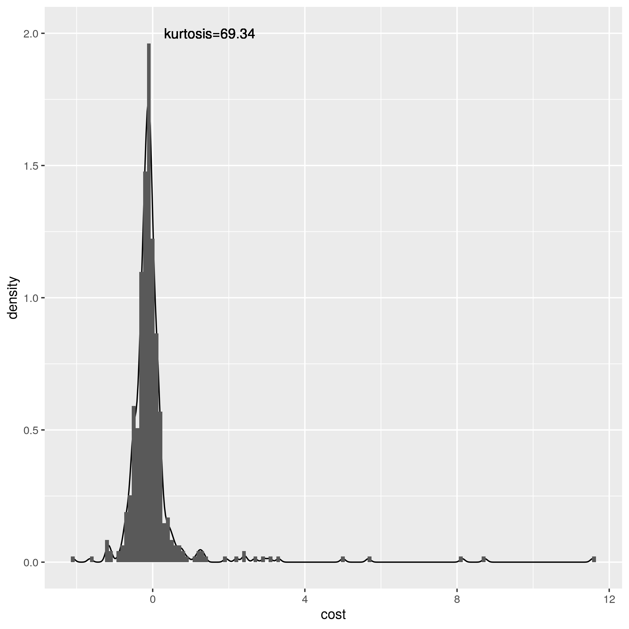
Figure 2: Density of Costly Disaster Shock

The three shocks recovered by ICA have kurtosis $(69.34,5.39,5.03)$. The density of $\hat{u}_{1}$ in Figure 2 shows that the shock has a heavy right tail. We estimate the impulse response functions by (i) iterating $A^{h}B$ as implied by the VAR, (ii) local projections using $\hat{u}$ obtained from ICA as shocks, and (iii) dynamic responses as implied by Choleski decomposition. These are labeled var, lp, and chol in Table 3. To provide some idea of precision of the estimated impulse responses, we report standard errors for the lp estimates as well 95% bootstrap confidence intervals using the vars package in R as rough guides. But note that our estimates $\hat{A}$ have non-standard distributions and results about bootstrap inference with heavy-tailed variables have only been considered in the univariate setting, see, for example, Davis and Wu (1997) and Wan and Davis (2022). Each local projections regression is of the HL type and hence inference is also non-standard. The standard errors should be interpreted with this caveat in mind.

The CD series has short memory and the effects of its own shock die out after one month. The shock induces a tightly estimated increase in uncertainty for three months and an increase in unemployment claims of two months. As a point of reference, an unemployment claims shock has an impact effect of 14.556 on itself, and an uncertainty shock has an impact effect of 8.898 on itself. The effects of a disaster shock on these economic variables are small, but they do exist. This reinforces the motivation of the HL model that infinite variance shocks can affect variables with finite variances.

It can be argued that the infinite variance nature of $u_{t1}$ makes the unit variance property of shocks identified by ICA unappealing. But it is easy to calibrate the shock to yield exactly a one percent change to the variable of interest without changing the shape of the impulse response function. With this data, the unit effect is associated with a shock of size 13.881, which is slightly larger than Katrina shock in 2005, which was of magnitude 11.56.

Table 3: Dynamic Effects of a Costly Disaster (CD) Shock

$h$	var	lp	lp.se	chol	chol.up	chol.dn
	Response of CD
1	13.88	13.88	0.00	13.88	18.45	7.90
2	2.63	2.61	1.87	2.65	3.85	1.23
3	-0.15	-0.31	0.82	-0.14	0.96	-1.24
4	-0.05	-0.09	0.34	-0.04	0.97	-0.90
5	-0.51	-0.44	0.35	-0.51	0.70	-1.54
6	-0.71	-0.56	0.32	-0.71	0.51	-1.63
	Response of Unemployment Claims
1	-0.27	-0.27	0.00	-0.09	1.32	-1.49
2	2.68	2.95	1.02	2.88	4.74	0.67
3	0.18	0.37	0.63	0.39	2.43	-1.04
4	-0.83	-0.72	0.83	-0.61	1.41	-2.85
5	-1.31	-1.03	1.08	-1.07	1.83	-3.68
6	-1.76	-1.64	1.15	-1.54	1.50	-4.33
	Response of JLN Uncertainty
1	0.87	0.87	0.00	1.01	2.21	0.16
2	2.65	2.57	0.58	2.89	4.95	1.36
3	2.28	2.02	0.86	2.56	5.11	0.67
4	1.26	0.74	1.10	1.56	4.64	-0.67
5	0.82	0.13	1.17	1.12	5.12	-1.78
6	0.28	-0.49	1.30	0.56	4.58	-2.81

Note: var are the dynamic response implied by the VAR using the ICA estimates. lp are responses estimated by local projections, and lp.se are the corresponding standard errors. chol are the dynamic responses using Choleski decomposition, with 95% confidence intervals defined by chol.up and chol.dn.

5.3 Example 3: Economic Shocks

covid-19 has been costly in health, social, and economic dimensions, but it has also created new challenges for data analysis. One problem discussed in Ng (2021) is that covid-19 is pervasive and persistent, and the principal components of economic data will be now spanned by common economic variations and covid-19. To isolate the economic factors, a suggestion was made to project each economic variable on covid indicators such as positivity rate, hospitalization, and deaths, then use the panel of ‘de-covid’ data to estimate the economic factors.

covid-19 also has implications for VAR estimation. Consider a two variable VAR in log payroll-employment (PAYEMS) and log consumption of durables (CD). The top panel of Figure 3 shows the response to a positive employment shock from a VAR estimated over the pre-covid sample of 1960:1-2020:2, while the second panel extends the sample to 2020:12. Adding ten months of post-covid data completely changed the shape of the impulse response functions. Lenza and Primiceri (2021) recognize that the covid-induced spikes in the data will distort VAR estimation and suggest to use Pareto priors for innovation variances to capture these spikes. Others such as Carriero, Clark, Marcellino, and Mertens (2021) model covid-19 as outliers.

Instead of specifying changes to the probability distribution of existing shocks, an alternative is to assume as in Ng (2021) that there is an additional ‘virus’ shock, say, $v$ in the post-covid sample. There are then two ways to proceed. The first is to de-covid all variables used in the VAR which would entail running $n(p+1)$ decovid regressions. By Frish-Waugh arguments, this is the same as adding covid indicators as exogenous variables to each equation. Note that these are not the same as running a VAR on $n$ de-covid variables, which would only entail $n$ decovid regressions. Results using the log changes in positive cases as $v$ are shown in the third panel of Figure 3. The dynamic responses are very similar to the ones in the top panel estimated on the pre-covid sample.

Removing the covid variations from the data before VAR estimation suppresses feedback from the economic variables to $v$ which could be restrictive. An alternative approach is to include a $v$ indicator in the VAR directly and order it first, resulting in a HL model with $(n+1)$ variables. In this case, interest is not in the dynamic effects of an infinite variance shock; but to isolate the economic variations so that the dynamic effects of economic shocks can be estimated in spite of the presence of covid-19. The results for the three variable VAR in the bottom panel of Figure 3 are again similar to the two step approach in the third panel. Whichever way we choose to control for covid variations, the exercise involves regressions with a finite variance variable on the left hand side and a heavy-tailed variable on the right hand side, and Proposition 1 is relevant to the interpretation of the estimates.

6 Conclusion

This paper provides a VAR framework that accommodates disaster-type events. The framework can be used to study the effects of disaster type shocks, as well as the effects of finite variance shocks in the presence of large rare events. Under the maintained assumption that the primitive shocks are independent, a disaster-type shock can be uniquely identified from the tail behavior and sign of the components estimated by ICA. An independence test for validity of the identifying restriction is also proposed. The test is valid even for exactly identified models and is of interest in its own right. The focus here is developing the HL framework and consistent estimation. Inference when the data have heavy tails remains an area for future research.

Figure 3: Dynamic Response of (PAYEMS, CS) to PAYEMS Shock

Bivariate VAR, PreCovid

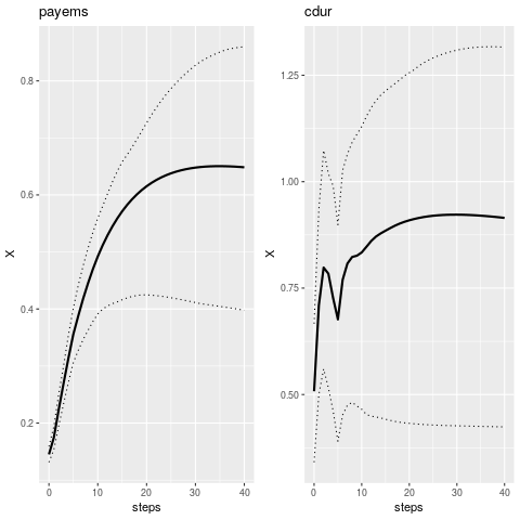
Bivariate VAR, PostCovid

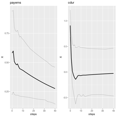
Bivariate VAR, Purging Covid Effects

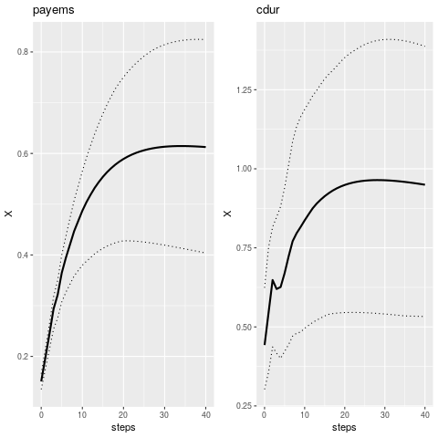
Three variable VAR, PostCovid

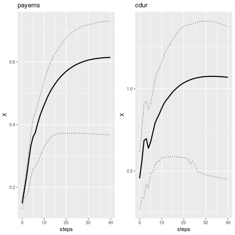
7 Appendix

7.1 Background on Distance Covariance

The distance covariance between two random vectors $X$ and $Y$ of dimensions $m$ and $n$, respectively, is given by

$${\mathcal{I}}(X,Y;w)=\int_{{\mathbb{R}}^{m+n}}\big{|}\varphi_{X,Y}(s,t)-\varphi_{X}(s)\,\varphi_{Y}(t)\big{|}^{2}w(s,t)ds\,dt\,,$$ (16)

where $w(s,t)>0$ is a weight function and $\varphi_{Z}(t)=E[\exp^{i(t,Z)}],\,t\in{\mathbb{R}}^{d}\,$ denotes the characteristic function for any random vector $Z\in{\mathbb{R}}^{d}$. It is assumed that the integral in (10) is finite, which certainly holds if $w(s,t)$ is a probability density function. One sees immediately that $X$ and $Y$ are independent if and only if ${\mathcal{I}}(X,Y;w)=0$ since in this case the joint characteristic function factors into the product of the respective marginal characteristic functions, $\varphi_{X,Y}(s,t)=\varphi_{X}(s)\,\varphi_{Y}(t)$ for all $(s,t)\in{\mathbb{R}}^{m+n}$. Now if the weight function factors into a product function, i.e., $w(s,t)=w_{1}(s)w_{2}(t)$, then under suitable moment conditions on $X$ and $Y$, ${\mathcal{I}}(X,Y,w)$ has the form

$$T(X,Y;w) = E[\hat{w}_{1}(X-X^{\prime})\,\hat{w}_{2}(Y-Y^{\prime})]+E[\hat{w}_{1}(X-X^{\prime})]E[\hat{w}_{2}(Y-Y^{\prime})]$$ (17)

$$-2\,E[\hat{w}_{1}(X-X^{\prime})\,\hat{w}_{2}(Y-Y^{\prime\prime})]\,,$$

where $\hat{w}_{1}(x)=\int_{{\mathbb{R}}^{m}}e^{i(s,x)}w_{1}(s)ds$, $\hat{w}_{2}(y)=\int_{{\mathbb{R}}^{n}}e^{i(t,y)}w_{1}(s)ds$, and $(X,Y),(X^{\prime},Y^{\prime}),(X^{\prime\prime},Y^{\prime\prime})$ are iid copies of $(X,Y)$. This relation is found by expanding the square in the integrand in (16) and using Fubini to interchange integration with expectation. Precise conditions on $w$ to perform these operations is given in Davis, Matsui, Mikosch, and Wan (2018). Suffice it to say that if $w_{i}$ is a probability density function, then application of Fubini requires no further conditions on the distributions of $X$ and $Y$. In order to avoid direct integration in (16), one can choose functions, $w_{i}$ which have an easily computable Fourier transform. Examples include the Gaussian density for which $\widetilde{w}_{i}(x)=\exp\{-\sigma^{2}\|x\|^{2}/2\}$ or a Cauchy density in which case $\widetilde{w}_{i}(x)=\exp\{-\sigma\|x\|_{1}\}$, where $\|x\|_{1}$ is the 1-norm. A popular choice for $w$ is

$$w(s,t)=\left(c_{m,\beta}|s|^{\beta+m}c_{n,\beta}|t|^{\beta+n}\right)^{-1}\,,$$ (18)

where $\beta\in(0,2)$, $c_{m,\beta}=\frac{2\pi{m/2}\Gamma(1-\beta/2)}{\beta 2^{\beta}\Gamma((\beta+m)/2)}$ (see Székely, Rizzo, and Bakirov (2007)). In this case, one has $\int_{\mathbb{R}}^{m}c_{m,\beta}^{-1}\left(1-\cos(s,x)\right)ds=|x|^{\beta}$, and provided $E(|X|^{\beta}+E|Y|^{\beta}+|X|^{\beta}|Y|^{\beta})<\infty$, then

$${\mathcal{I}}(X,Y;w) = E[|X-X^{\prime}|^{\beta}|Y-Y^{\prime}|^{\beta})]+E[|X-X^{\prime}|^{\beta}]E[|Y-Y^{\prime}|^{\beta}]$$ (19)

$$-2\,E[|X-X^{\prime}|^{\beta}|Y-Y^{\prime\prime}|^{\beta}]\,.$$

Notice that with this choice of $w$, ${\mathcal{I}}$ is invariant under orthogonal transformations on $X$ and $Y$ and is scale homogeneous under positive scaling. The most common choice for $\beta$ is the value 1, which requires a finite mean. In our heavy-tailed framework, we have assumed the tail-index $\alpha\in(1,2)$ so the integral in (16) is finite and formula (19) is valid (if $X$ and $Y$ are independent) using the above weight function $w$ with $\beta=1$. However, in order to extend the results to heavier tails, such as Cauchy, then one can choose a smaller $\beta$, which is difficult to identify in practice, or use the the Gaussian density function. As noted in Davis, Matsui, Mikosch, and Wan (2018), the weight function in (11) can have potential limitations when applied to estimated residuals in the finite variance case.

Based on data $(X_{1},Y_{1}),\ldots,(X_{T},Y_{T})$ from $(X,Y)$, the general distance covariance in (16) can be estimated by replacing the characteristic function with their empirical counterparts. Using the $w$ given in (18), we obtain the estimate

$$\hat{\mathcal{I}}(X,Y;w) = \frac{1}{T^{2}}\sum_{i=1}^{T}\sum_{j=1}^{T}|X_{i}-X_{j}|^{\beta}\,|Y_{i}-Y_{j}|^{\beta}+\left(\frac{1}{T^{2}}\sum_{i=1}^{T}\sum_{j=1}^{T}|X_{i}-X_{j}|^{\beta}\right)\left(\frac{1}{T^{2}}\sum_{i=1}^{T}\sum_{j=1}^{T}|Y_{i}-Y_{j}|^{\beta}\right)$$

$$~{}~{}~{}-2\frac{1}{T^{3}}\sum_{i=1}^{T}\sum_{j=1}^{T}\sum_{k=1}^{T}|X_{i}-X_{j}|^{\beta}\,|Y_{i}-Y_{k}|^{\beta}\,,$$

which can be shown to be consistent for ${\mathcal{I}}(X,Y;w)$ by the ergodic theorem applied to the empirical characteristic function. The limit theory for $T\hat{\mathcal{I}}(X,Y;w)$, under the assumption that $X$ and $Y$ are independent can be found in Székely, Rizzo, and Bakirov (2007) in the iid case and in in Davis, Matsui, Mikosch, and Wan (2018) a time series setting when $\{(X_{t},Y_{t})\})$ is a stationary time series. The latter also considers the limit theory of $\sqrt{T}\left(\hat{\mathcal{I}}(X,Y;w)-{\mathcal{I}}(X,Y;w)\right)$, when $X$ and $Y$ are not independent.

7.2 Proofs

We now consider an array of models given by $Y_{t,T}=A_{T}Y_{t-1,T}+B_{T}u_{t}$, where

• $A_{21,T}=\frac{a_{21}}{T^{\theta}}$ and $B_{21,T}=\frac{b_{21}}{T^{\theta}}$, with $\theta=1/\alpha-1/2$.

• $u_{t1}$ has Pareto-like tails, $\mathbb{E}[u_{t1}]=0$ if it exists and has dispersion 1 so that $T\mathbb{P}(|u_{t1}|>T^{1/\alpha})\rightarrow 1$ and $u_{t2}\sim(0,1)$.

In other words, for fixed $T$, the time series $\{Y_{t,T},\,t\in\mathbb{Z}\}$ satisfies the VAR(1) equations with coefficient matrix $A_{T}$. The time series of observations, $Y_{1},\ldots,Y_{T}$ are then considered to come from this model. To lighten the notation going forward, we will often suppress the dependence of $Y_{t}$ on $T$.

Claim 1.

We will first show that the assumptions imply that $\frac{1}{T}\sum Y_{t2,T}^{2}\smash{\mathop{\longrightarrow}\limits^{d}}S^{*}_{2}$ where $S^{*}_{2}$ is random or a constant, and hence the sample variance of $Y_{t2}$ is convergent.

From the causal MA representation, we have

$$Y_{t}=\sum_{j=0}^{\infty}A_{T}^{j}Bu_{t-j}\,,$$

which can be expressed component-wise as

$$Y_{t1} = \sum_{j=0}^{\infty}c_{j,11}u_{t-j,1}+\sum_{j=0}^{\infty}c_{j,12}u_{t-j,2}$$ (20)

$$Y_{t2} = \frac{1}{T^{\theta}}\sum_{j=0}^{\infty}c_{j,21}u_{t-j,1}+\sum_{j=0}^{\infty}c_{j,22}u_{t-j,2}\,,$$ (21)

where the $c_{j,ik}$ depend on $T$ but converge (as $T\to\infty$) to finite limits that decay as a function of the lag $j$ at an exponential rate. For example, $(c_{0,11},c_{0,12})$ corresponds to the first row of the matrix $B$, while $(c_{0,21},c_{0,22})=(b_{21},B_{22})$.

Since $\theta=1/\alpha-1/2$, $2\theta+1=2/\alpha$, and $1+\theta=1/\alpha+1/2$, the sample mean of the $Y_{t2}$, normalized by $\sqrt{T}$, converges in distribution even if the population variance is infinite. We have

$$\frac{1}{\sqrt{T}}\sum_{t=1}^{T}Y_{t2} = \sum_{j=0}^{\infty}c_{j,21}\left(\frac{1}{T^{1/\alpha}}\sum_{t=1}^{T}u_{t-j,1}\right)+\sum_{j=0}^{\infty}c_{j,22}\left(\frac{1}{\sqrt{T}}\sum_{t=1}^{T}u_{t-j,2}\right)$$

$$\smash{\mathop{\longrightarrow}\limits^{d}} \left(\sum_{j=0}^{\infty}c_{j,12}^{*}\right)S_{u}+\left(\sum_{j=0}^{\infty}c_{j,22}^{*}\right)N_{u}=:S^{*}_{Y,2}$$

where $c_{j,2i}^{*}=\lim_{T\to\infty}c_{j,2i}$, $i=1,2$, and $S_{u}$ is a stable random variable with index $\alpha$ that is independent of $N_{u}$, a standard normal random variable. The sample second moment also converges. To see this, we have

$$\frac{1}{T}\sum_{t=1}^{T}Y_{t2}^{2} = \sum_{j=0}^{\infty}c_{j,21}^{2}\left(\frac{1}{T^{2/\alpha}}\sum_{t=1}^{T}u_{t-j,1}^{2}\right)+\sum_{j\neq k=0}^{\infty}c_{j,21}c_{k,21}\left(\frac{1}{T^{2/\alpha}}\sum_{t=1}^{T}u_{t-j,1}u_{t-k,1}\right)$$ (22)

$$+\sum_{j=0}^{\infty}c_{j,22}^{2}\left(\frac{1}{T}\sum_{t=1}^{T}u_{t-j,2}^{2}\right)+\sum_{j\neq k=0}^{\infty}c_{j,22}c_{k,22}\left(\frac{1}{T}\sum_{t=1}^{T}u_{t-j,2}u_{t-k,2}\right)$$

$$+\sum_{j,k=0}^{\infty}c_{j,21}c_{k,22}\left(\frac{1}{T^{1/\alpha+1/2}}\sum_{t=1}^{T}u_{t-j,1}u_{t-k,2}\right)$$

$$\smash{\mathop{\longrightarrow}\limits^{d}} \left(\sum_{j=0}^{\infty}(c_{j,21}^{*})^{2}\right)S_{uu}+\sum_{j=0}^{\infty}(c_{j,22}^{*})^{2}=:S^{*}_{YY,2}\,,$$

where $S_{uu}$ is a stable random variable with index $\alpha/2$. The last line follows essentially from Lemma 1, which shows that for $j\neq k$,

$$\frac{1}{T^{1/\alpha}\log T}\sum_{t=1}^{T}u_{t-j,1}u_{t-k,1}=O_{p}(1)$$ (23)

$$\frac{1}{T^{1/\alpha}}\sum_{t=1}^{T}u_{t-j,1}u_{t-k,2}=O_{p}(1),$$ (24)

$$\frac{1}{T}\sum_{t=1}^{T}u_{t-j,2}u_{t-k,2}=o_{p}(1)$$ (25)

by the ergodic theorem. Using the ideas in Davis and Resnick (1986) and the continuous mapping theorem, it is straightforward to obtain the limit in the last line upon summing out $j$ and $k$.

Proof of Proposition 1

We first note that the OLS estimate of $A$ is given by

$$\hat{A}=\sum_{t=2}^{T}Y_{t}Y_{t-1}^{\prime}\left(\sum_{t=1}^{T-1}Y_{t}Y_{t}^{\prime}\right)^{-1}$$ (26)

and hence

$$\hat{A}-A=\sum_{t=2}^{T}e_{t}Y_{t-1}^{\prime}\left(\sum_{t=1}^{T-1}Y_{t}Y_{t}^{\prime}\right)^{-1}$$ (27)

(For simplicity, we have terminated the second sum in (26) and (27) at $T-1$ instead of $T$, but this has no bearing on the asymptotics.) We begin by analyzing the terms in the matrix of cross products given by $\sum_{t=1}^{T-1}Y_{t}Y_{t}^{\prime}$. From (22), we can write

$$\sum_{t=1}^{T}Y_{t2}^{2}=TS_{22,T},$$

where $S_{22,T}=\frac{1}{T}\sum_{t=1}^{T}Y_{t2}^{2}\smash{\mathop{\longrightarrow}\limits^{d}}S^{*}_{YY,2}$. The same argument as above shows that $T^{-2/\alpha}\sum_{t=1}^{T}Y_{t1}^{2}\smash{\mathop{\longrightarrow}\limits^{d}}S^{*}_{YY,1}$, so that

$$T^{2/\alpha}\sum_{t=1}^{T}Y_{t1}^{2}=T^{2/\alpha}S_{11,T},$$

with $S_{11,T}\smash{\mathop{\longrightarrow}\limits^{d}}S^{*}_{YY,1}$. Now applying the same arguments as before,

$$\frac{1}{T^{1/\alpha+1/2}}\sum_{t=1}^{T}Y_{t1}Y_{t2} = \sum_{j,k=0}^{\infty}c_{j,11}c_{k,21}\left(\frac{1}{T^{2/\alpha}}\sum_{t=1}^{T}u_{t-j,1}u_{t-k,1}\right)+\sum_{j,k=0}^{\infty}c_{j,12}c_{k,21}\left(\frac{1}{T^{2/\alpha}}\sum_{t=1}^{T}u_{t-j,2}u_{t-k,1}\right)$$

$$+\sum_{j,k=0}^{\infty}c_{j,11}c_{k,22}\left(\frac{1}{T^{1/\alpha+1/2}}\sum_{t=1}^{T}u_{t-j,1}u_{t-k,2}\right)$$

$$+\sum_{j,k=0}^{\infty}c_{j,12}c_{k,22}\left(\frac{1}{T^{1/\alpha+1/2}}\sum_{t=1}^{T}u_{t-j,2}u_{t-k,2}\right)$$

$$\smash{\mathop{\longrightarrow}\limits^{d}} \left(\sum_{j=0}^{\infty}c_{j,11}^{*}c_{j,21}^{*}\right)S_{uu}=:S^{*}_{YY,12}\,,$$

where we have made use of (23)–(25) once again. We write

$$\sum_{t=1}^{T}Y_{t1}Y_{t2}=T^{1/\alpha+1/2}S_{12,T},$$

where $S_{12,T}\smash{\mathop{\longrightarrow}\limits^{d}}S^{*}_{YY,12}$. It follows that

$$(\sum_{t=1}^{T}Y_{t}Y_{t}^{\prime})^{-1}=\frac{1}{\text{det}}\begin{pmatrix}\sum_{t=1}^{T}Y_{t2}^{2}&-\sum_{t=1}^{T}Y_{t1}Y_{t2}\\ -\sum_{t=1}^{T}Y_{t1}Y_{t-1,2}&\sum_{t=1}^{T}Y_{t1}^{2}\end{pmatrix}=\frac{1}{\text{det}}\begin{pmatrix}TS_{22,T}&-T^{1/\alpha+1/2}S_{12,T}\\ -T^{1/\alpha+1/2}S_{12,T}&T^{2/\alpha}S_{11,T}\end{pmatrix}\,,$$

where $det=T^{2/\alpha+1}D_{T}$ and $D_{T}=(S_{11,T}S_{22,T}-S_{12,T}^{2})\smash{\mathop{\longrightarrow}\limits^{d}}D_{\infty}:=S_{YY,1}^{*}S_{YY,2}^{*}-(S_{YY,12}^{*})^{2}$. The inverse can then be written more concisely as

$$(\sum_{t=1}^{T}Y_{t}Y_{t}^{\prime})^{-1}=\frac{1}{D_{T}}\begin{pmatrix}T^{-2/\alpha}S_{22,T}&-T^{-1/\alpha-1/2}S_{12,T}\\ -T^{-1/\alpha-1/2}S_{12,T}&T^{-1}S_{11,T}\end{pmatrix}\,.$$ (28)

Estimation of the $Y_{1}$ equation

We have

$$(T\log T)^{-1/\alpha}\sum_{t=2}^{T}e_{t1}Y_{t-1,1} = \sum_{j=0}^{\infty}c_{j,11}(T\log T)^{-1/\alpha}\sum_{t=2}^{T}u_{t-1-j,1}(u_{t1}B_{11}+u_{t2}B_{12})$$ (29)

$$+\sum_{j=0}^{\infty}c_{j,12}(T\log T)^{-1/\alpha}\sum_{t=2}^{T}u_{t-1-j,2}(u_{t1}B_{11}+u_{t2}B_{12})$$

$$= \sum_{j=0}^{\infty}c_{j,11}(T\log T)^{-1/\alpha}\sum_{t=2}^{T}u_{t-1-j,1}u_{t1}B_{11}+o_{p}(1)$$

$$\smash{\mathop{\longrightarrow}\limits^{d}} S_{eY,11}.$$

Next

$$T^{-1/\alpha}\sum_{t=2}^{T}e_{t1}Y_{t-1,2} = \sum_{j=0}^{\infty}c_{j,21}T^{-2/\alpha+1/2}\sum_{t=2}^{T}u_{t-1-j,1}(u_{t1}B_{11}+u_{t2}B_{12})$$ (30)

$$+\sum_{j=0}^{\infty}c_{j,22}T^{-1/\alpha}\sum_{t=2}^{T}u_{t-1-j,2}(u_{t1}B_{11}+u_{t2}B_{12})$$

$$= \sum_{j=0}^{\infty}c_{j,22}T^{-1/\alpha}\sum_{t=2}^{T}u_{t-1-j,2}u_{t1}B_{11}+o_{p}(1)$$

$$\smash{\mathop{\longrightarrow}\limits^{d}} S_{eY,12}.$$

Estimation of the $Y_{2}$ equation

Using the representation in (20), it is relatively straightforward to show

$$T^{-1/\alpha}\sum_{t=2}^{T}e_{t2}Y_{t-1,1} = \bigg{(}\frac{b_{21}}{T^{\theta+1/\alpha}}\sum_{t=2}^{T}Y_{t-1,1}u_{t1}+B_{22}T^{-1/\alpha}\sum_{t=2}^{T}u_{t2}Y_{t-1,1}\bigg{)}\smash{\mathop{\longrightarrow}\limits^{d}}B_{22}S_{Yu,21}=:S_{eY,21}$$

since $(\log T)^{1/\alpha}/T^{\theta}\rightarrow 0$. Furthermore, since $\frac{(T\log T)^{1/\alpha}}{T^{2/\alpha-1/2}}=\frac{(\log T)^{1/\alpha}}{T^{\theta}}\rightarrow 0$,

$$\frac{1}{\sqrt{T}}\sum_{t=2}^{T}e_{t2}Y_{t-1,2} = \sum_{j=0}^{\infty}c_{j,21}\frac{1}{T^{1/\alpha}}\sum_{t=2}^{T}u_{t-j-1,1}\left(\frac{b_{21}}{T^{\theta}}u_{t1}+B_{22}u_{t2}\right)$$

$$+\sum_{j=0}^{\infty}c_{j,22}\frac{1}{T^{1/2}}\sum_{t=2}^{T}u_{t-j-1,2}\left(\frac{b_{21}}{T^{\theta}}u_{t1}+B_{22}u_{t2}\right)$$

$$\smash{\mathop{\longrightarrow}\limits^{d}} B_{22}S_{Yu,12}+b_{21}S_{uu,21}+B_{22}N_{u2}=:S_{eY,22}\,,$$

where $S_{Yu,12},S_{uu,21}$ are stable with index $\alpha$ and $N_{u2}$ is normally distributed.

Summarizing, we have, using an obvious notation,

$$\sum_{t=2}^{T}e_{t}Y_{t-1}^{\prime}=\begin{pmatrix}\sum_{t=2}^{T}e_{t1}Y_{t-1,1}&\sum_{t=2}^{T}e_{t1}Y_{t-1,2}\\ \sum_{t=2}^{T}e_{t2}Y_{t-1,1}&\sum_{t=2}^{T}e_{t1}Y_{t-1,2}\end{pmatrix}=\begin{pmatrix}(T\log T)^{1/\alpha}\widetilde{S}_{11,T}&T^{1/\alpha}\widetilde{S}_{12,T}\\ T^{1/\alpha}\widetilde{S}_{21,T}&T^{1/2}\widetilde{S}_{22,T}\end{pmatrix}\,,$$

so that $\hat{A}-A$ is

$$=\frac{1}{D_{T}}\begin{pmatrix}(T\log T)^{1/\alpha}\widetilde{S}_{11,T}&T^{1/\alpha}\widetilde{S}_{12,T}\\ T^{1/\alpha}\widetilde{S}_{21,T}&T^{1/2}\widetilde{S}_{22,T}\end{pmatrix}\begin{pmatrix}T^{-2/\alpha}S_{22,T}&-T^{-1/\alpha-1/2}S_{12,T}\\ -T^{-1/\alpha-1/2}S_{12,T}&T^{-1}S_{11,T}\end{pmatrix}\,.$$

Since $-1/\alpha+1/2<0$ and $1-1/\alpha-1/2<0$, we conclude

$$\sqrt{T}(\hat{A}_{11}-A_{11}) \smash{\mathop{\longrightarrow}\limits^{d}} S_{A,11}:=-S_{eY,12}S_{YY,12}^{*}/D_{\infty}$$

$$T^{1-1/\alpha}(\hat{A}_{12}-A_{12}) \smash{\mathop{\longrightarrow}\limits^{d}} S_{A,12}:=S_{eY,12}S_{YY,11}^{*}/D_{\infty}$$

$$T^{1/\alpha}(\hat{A}_{21}-A_{21}) \smash{\mathop{\longrightarrow}\limits^{d}} S_{A,21}:=(S_{eY,21}S_{YY,22}^{*}-S_{eY,22}S_{YY,12}^{*})/D_{\infty}$$

$$\sqrt{T}(\hat{A}_{22}-A_{22}) \smash{\mathop{\longrightarrow}\limits^{d}} S_{A,22}:=(S_{eY,22}S_{YY,11}^{*}-S_{eY,21}S_{YY,12}^{*})/D_{\infty}.$$

$\Box$

Proof of Proposition 3

The proof relies on an application of Theorem 3.3 in Davis and Fernandes (2022), which considers consistency for the unmixing matrix in an ICA model with noise. Observe that

$$\hat{e}_{t}=Y_{t}-\hat{Y}_{t}=e_{t}+(A-\hat{A})Y_{t-1}=Bu_{t}+r(T)Y_{t-1}\,,$$ (31)

where $r(T)=A-\hat{A}=o_{P}(1)$. By the independence of $u_{t}$ with $Y_{t-1}$ it follows that the components of $E|u_{t}||Y_{t-1}|<\infty$. Hence, in order to apply Theorem 3.3, it suffices to show that

$$\hat{\Sigma}^{-1}_{e}-\hat{\Sigma}^{-1}_{\hat{e}}\overset{p}{\to}0\,.$$ (32)

We first show

$$\hat{\Sigma}_{e}-\hat{\Sigma}_{\hat{e}}\overset{p}{\to}0\,.$$ (33)

From (31),

$$\hat{\Sigma}_{e}-\hat{\Sigma}_{\hat{e}} = -(\hat{A}-A)\hat{\Sigma}_{y}(\hat{A}-A)^{\prime}+(\hat{A}-A)T^{-1}\sum_{t=1}^{T}Y_{t-1}e_{t}^{\prime}+T^{-1}\sum_{t=1}^{T}e_{t}Y_{t-1}^{\prime}(\hat{A}-A)^{\prime},$$

where $\hat{\Sigma}_{y}$ is the sample covariance matrix of $Y_{t-1},\,t=1,\ldots,T$. Using the relations for $\hat{A}-A$ in Proposition 1, and the calculations leading to the limit in (28), it follows that

$$(\hat{A}-A)\hat{\Sigma}_{y}(\hat{A}-A)^{\prime}\overset{p}{\to}0\,.$$

Similarly, applying (29)–(30), it is straightforward to also show that

$$(\hat{A}-A)T^{-1}\sum_{t=1}^{T}Y_{t-1}e_{t}^{\prime}+T^{-1}\sum_{t=1}^{T}e_{t}Y_{t-1}^{\prime}(\hat{A}-A)^{\prime}\overset{p}{\to}0\,,$$

which proves (33). To finish the proof, we note the following relations

$$\frac{1}{T}\sum_{t=1}^{T}e_{t1}^{2} = T^{2/\alpha-1}B_{11}^{2}S_{11,T}+B_{12}^{2}\sigma_{2}^{2}+o_{P}(1)$$ (34)

$$\frac{1}{T}\sum_{t=1}^{T}e_{t2}^{2} = b_{21}^{2}S_{11,T}+B_{22}^{2}\sigma_{2}^{2}+o_{P}(1)$$ (35)

$$\frac{1}{T}\sum_{t=1}^{T}e_{t1}e_{t2} = T^{1/\alpha-1/2}B_{11}b_{21}S_{11,T}+B_{11}B_{22}\sigma_{2}^{2}+o_{P}(1)\,,$$ (36)

where $S_{11,T}=T^{-2/\alpha}\sum_{t=1}^{T}u_{t1}^{2}=O_{P}(1)$, and $\sigma_{2}^{2}=\mbox{var}(u_{t2})$. In view of (33), the exact same relations hold for the corresponding entries of $\hat{\Sigma}_{\hat{e}}$. The determinant of both sample covariance matrices is then of order

$$|\hat{\Sigma}_{e}|=T^{2/\alpha-1}B_{11}^{2}S_{11,T}B_{22}\sigma_{2}^{2}+O_{P}(T^{1/\alpha-1/2})\,.$$

Since $\hat{\Sigma}^{-1}_{e}=\frac{1}{|\hat{\Sigma}_{e}|}\widetilde{\Sigma}_{e}$, where

$$\widetilde{\Sigma}_{e}=\begin{pmatrix}T^{-1}\sum_{t=1}^{T}e_{t2}^{2}&-T^{-1}\sum_{t=1}^{T}e_{t1}e_{t2}\\ -T^{-1}\sum_{t=1}^{T}e_{t1}e_{t2}&T^{-1}\sum_{t=1}^{T}e_{t1}^{2}\end{pmatrix}\,,$$

with a similar expression for $\hat{\Sigma}^{-1}_{\hat{e}}$, we have

$$\hat{\Sigma}^{-1}_{e}-\hat{\Sigma}^{-1}_{\hat{e}}=\left(\frac{1}{|\hat{\Sigma}_{e}|}-\frac{1}{|\hat{\Sigma}_{\hat{e}}|}\right)\widetilde{\Sigma}_{e}-\frac{1}{|\hat{\Sigma}_{\hat{e}}|}\left(\widetilde{\Sigma}_{e}-\widetilde{\Sigma}_{\hat{e}}\right)\,.$$

The second converges to in probability by (32) and the fact that he determinant goes to infinity in probability. To show the first term converges to 0, since $|\hat{\Sigma}_{e}|/|\hat{\Sigma}_{\hat{e}}|\overset{p}{\to}1$, it suffices to show that the matrix $\hat{\Sigma}_{e}^{-1}$ remains bounded. But

$$\hat{\Sigma}_{e}^{-1}=W\hat{\Sigma}_{u}^{-1}W^{\prime}\,,$$

where $\hat{\Sigma}$ is the sample covariance matrix of $u_{1},\ldots,U_{t}$. A straight forward calculation shows that

$$\hat{\Sigma}_{u}^{-1}\overset{p}{\to}\begin{pmatrix}0&0\\ 0&\sigma_{2}^{-2}\end{pmatrix}$$

and hence $\hat{\Sigma}_{e}^{-1}$ is bounded in probability as claimed. This establishes (32) which completes the proof of the proposition. $\Box$

Proof of Lemma 3

Using (34), we see that

$$e_{t1}^{c}=\frac{e_{t1}}{\sqrt{T^{-1}\sum_{s=1}^{T}e_{s1}^{2}}}\sim\frac{e_{t1}}{\sqrt{T^{2/\alpha-1}B_{11}^{2}S_{11,T}}}\,,$$

which gives the asserted representation for $e_{t1}^{c}$. Also from (35) and (36), we find that

$$c_{T}\sim\frac{b_{21}}{T^{1/\alpha-1/2}B_{11}}\,,$$

as $T\to\infty$. It follows from (34)–(36) that

$$T^{-1}\sum_{s=1}^{T}(e_{s2}-c_{T}e_{s1})^{2} = T^{-1}\sum_{s=1}^{T}\left(e_{s2}^{2}-2c_{T}e_{s1}e_{s2}+c_{T}^{2}e_{s2}^{2}\right)$$

$$\sim B_{22}^{2}\sigma_{2}^{2}\,.$$

Since $c_{T}\overset{p}{\to}0$, we conclude

$$e^{c}_{t2}=\frac{e_{t1}}{\sqrt{T^{-1}\sum_{s=1}^{T}(e_{s2}-c_{T}e_{t1})^{2}}}\sim\frac{e_{t2}-c_{T}e_{t1}}{|B_{22}|\sigma_{2}}\sim\frac{B_{22}}{|B_{22}|\sigma_{2}}u_{t2}\,,$$

as claimed. $\Box$

References

- (1)
- Amengual, Fiorentini, and Sentana (2021) Amengual, D., G. Fiorentini, and E. Sentana (2021): “Moment Tests of Independent Components,” unpublished manuscript CEMFI.
- Amsler and Schmidt (2012) Amsler, C., and P. Schmidt (2012): “Tests of Short Memory with Thick-Tailed Errors,” Journal of Business and Economic Statistics, 30:3, 381–390.
- Bach and Jordan (2001) Bach, F., and M. Jordan (2001): “Kernel Independent Component Analysis,” UNiversity of California, Berkeley, Computer Science Division,Technical Report CSD-01-1166.
- Beare and Toda (2020) Beare, B. K., and A. A. Toda (2020): “On the emergence of a power law in the distribution of COVID-19 cases,” Physica D. Nonlinear phenomena, 412:132649.
- Blattberg and Sargent (1971) Blattberg, R., and T. Sargent (1971): “Regression with Non-Gaussian Stable Distributions: Some Sampling Results,” Econometrica, 39:3, 501–510.
- Botzen, Deschenes, and Sanders (2019) Botzen, W., O. Deschenes, and M. Sanders (2019): “The Economic Impacts of Natural Disasters: A Review of Models and Empirical Studies,” Review of Environmental Economics and Policy, 13:2, 167–188.
- Carriero, Clark, Marcellino, and Mertens (2021) Carriero, A., T. Clark, M. Marcellino, and E. Mertens (2021): “Addressing COVID-19 Outliers in BVARs with Stochastic Volatility,” mimeo.
- Chen and Bickel (2006) Chen, A., and P. Bickel (2006): “Efficient Independent Component Analysis,” Annals of Statistics, 34:6, 2825–2855.
- Cohen, Davis, and Samorodnitsky (2020) Cohen, J. E., R. A. Davis, and G. Samorodnitsky (2020): “Heavy-tailed distributions, correlations, kurtosis and Taylor’s Law of fluctuation scaling,” Proceedings of the Royal Society A, 476(2244), 20200610.
- Comon (1994) Comon, P. (1994): “Independent Component Analysis: A New Concept,” Signal Process, 36:3, 287–313.
- Davis and Fernandes (2022) Davis, R., and L. Fernandes (2022): “Independent Component Analysis with Heavy Tails using Distance Covariance,” manuscript in preparation, Columbia University, http://www.stat.columbia.edu/~rdavis/papers/DavisFernandesDraft2022.pdf.
- Davis, Matsui, Mikosch, and Wan (2018) Davis, R. A., M. Matsui, T. Mikosch, and P. Wan (2018): “Applications of distance correlation to time series,” Bernoulli, 24(4A), 3087–3116.
- Davis and Resnick (1986) Davis, R. A., and S. Resnick (1986): “Limit Theory for the Sample Correlation Function of Moving Averages,” The Annals of Statistics, 14, 533–558.
- Davis and Wu (1997) Davis, R. A., and W. Wu (1997): “Bootstrapping M-estimates in regression and autoregression with infinite variance,” Statistica Sinica, pp. 1135–1154.
- Dufour and Kims (2014) Dufour, J. M., and J. K. Kims (2014): “Heavy-Tails and Paretian Distributions in Econometrics,” Journal of Econometrics, 181.
- Eriksson and Koivunen (2003) Eriksson, J., and V. Koivunen (2003): “Charcteristic-Function Based Independent Component Analysis,” Signal Processing, 83:10, 2195–2208.
- Gouriéroux, Monfort, and Renne (2017) Gouriéroux, C., A. Monfort, and J. Renne (2017): “Statistical Inference for Independent Component Analysis: Application to Structural VAR Models,” Journal of Econometrics, 196, 111–126.
- Hastie and Tibshirani (2003) Hastie, T., and R. Tibshirani (2003): “Independent Component Analysis Through Product Density Estimation,” in Advances in Neural Information Processing, vol. 15, pp. 649–656.
- Herwatz (2019) Herwatz, H. (2019): “Long-run Neutrality of Demand Shocks: Revisiting Blanchard and Quah (1989) with Independent Structural Shocks,” Journal of Applied Econometrics, 34, 811–819.
- Hill (1975) Hill, B. (1975): “A Simple General Approach to Inference about the Tail of a Distribution,” The Annals of Statistics, 3, 1163–1173.
- Hyvaninen, Karhunen, and Oja (2001) Hyvaninen, A., J. Karhunen, and E. Oja (2001): Independent Component Analysis. Wiley, New York.
- Hyvaninen and Oja (2000) Hyvaninen, A., and E. Oja (2000): “Independent Component Analyesis Algorithms and Applications,” Neural Networks, 13:4-5, 411–430.
- Hyvarinen (2013) Hyvarinen, A. (2013): “Independent Component Analaysis: Recent Advances,” Philosophical Transactions Roayl Society Series A,, 371:20110534.
- Hyvarinen, Zhang, Shimizu, and Hoyer (2010) Hyvarinen, A., K. Zhang, S. Shimizu, and P. Hoyer (2010): “Estimation of a Stuctural Vector-Autoregression Model Using Non-Gaussianity,” Journal of Machine Learning Research, 11, 1709–1731.
- Jorda (2005) Jorda, O. (2005): “Estimation and Inference of Impulse Responses by Local Projections,” American Economic Review, 95, 161–182.
- Josse and Holmes (2016) Josse, J., and S. Holmes (2016): “Measuring Multivariate Assocaition and Beyond,” Statistical Surveys, 10, 132–167.
- Jurado, Ludvigson, and Ng (2015) Jurado, K., S. C. Ludvigson, and S. Ng (2015): “Measuring Uncertainty,” American Economic Review, 105(3), 1117–1216.
- Kadiyala (1972) Kadiyala, K. R. (1972): “Regression with Non-Gaussian Stable Disturbances: Some Sampling Results,” Econometrica, 40:4, 719–722.
- Kilian and Lutkepohl (2017) Kilian, L., and H. Lutkepohl (2017): Structural Vector Autoregressive Analysis. Cambridge University Press.
- Lanne, Meitz, and Saikkonen (2017) Lanne, M., M. Meitz, and P. Saikkonen (2017): “Identification and Estimation of Non-Gaussian Structural Autoregressions,” Journal of Econometrics, 196:2, 288–304.
- Lenza and Primiceri (2021) Lenza, M., and G. Primiceri (2021): “How to Estimate a VAR after March 2020,” Journal of Applied Econometrics, forthcoming.
- Ludvigson, Ma, and Ng (2021a) Ludvigson, S., S. Ma, and S. Ng (2021): “Covid-19 and the Costs of Deadly Disasters,” AEA Papers and Proceedings, 111, 360–370.
- Ludvigson, Ma, and Ng (2021b) (2021b): “Uncertainty and Business Cycles: Exogenous Impulse or Endogenous Response?,” American Economic Journal: Macroeconomics, 13:4, 369–410.
- Matteson and Tsay (2017) Matteson, D., and R. S. Tsay (2017): “Independent Component Analysis via Distance Covariance,” Journal of the American Statistical Association, 112:518, 623–637.
- Maxand (2020) Maxand, S. (2020): “Identification of Independent Structural Shocks in the Presence of Multiple Gaussian Components,” Econometrics and Statistics.
- Mikosch and de Vries (2013) Mikosch, T., and C. G. de Vries (2013): “Heavy Tails of OLS,” Journal of Econometrics, 172, 205–221.
- Moneta, Entner, Hoyer, and Coad (2013) Moneta, A., D. Entner, P. Hoyer, and A. Coad (2013): “Causal Inference by Independent Component Analysis: Theory and Applications,” Oxford Bulletin of Economics and Statistics, 75:5, 705–730.
- Montiel Olea and Plagborg-Moller (2022) Montiel Olea, J., and M. Plagborg-Moller (2022): “SVAR Identification from Higher Moments: Has the Simultaneous Causality Problem Been Solved,” AEA Papers and Proceedings, forthcoming.
- Mueller and Watson (2017) Mueller, U. K., and M. W. Watson (2017): “Low Frequency Econometrics,” in Advances in Economics and Econometrics, vol. 2, p. p53. Cambridge University Press.
- Ng (2021) Ng, S. (2021): “Modeling Macroeconomic Variations After COVID-19,” arXiv:2103.02732.
- Paolella, Renault, Samorodnitsky, and Varedas (2013) Paolella, M., E. Renault, G. Samorodnitsky, and D. Varedas (2013): “Latest Developmentes on Heavy-Tailed Distributions,” Journal of Econometrics, 172.
- Samworth and Yuan (2012) Samworth, R., and M. Yuan (2012): “Independent Component Analysis Via Nonparametric Maximimum Likelhood Estimation,” Annals of Statistics, 40:6, 2973–3002.
- Stock and Watson (2015) Stock, J., and M. W. Watson (2015): “Factor Models for Macroeconomics,” in Handbook of Macroeconomics, ed. by J. B. Taylor, and H. Uhlig, vol. 2. North Holland.
- Székely, Rizzo, and Bakirov (2007) Székely, G. J., M. L. Rizzo, and N. K. Bakirov (2007): “Measuring and Testing Dependence by Correlation of Distances,” Annals of Statistics, 35, 2769–2794.
- Wan and Davis (2022) Wan, P., and R. Davis (2022): “Goodness-of-Fit Testing for Time Series Models via Distance Covariance,” Journal of Econometrics, forthcoming.