A Framework for Machine Learning of
Model Error in Dynamical Systems

Abstract.

The development of data-informed predictive models for dynamical systems is of widespread interest in many disciplines. We present a unifying framework for blending mechanistic and machine-learning approaches to identify dynamical systems from noisily and partially observed data. We compare pure data-driven learning with hybrid models which incorporate imperfect domain knowledge, referring to the discrepancy between an assumed truth model and the imperfect mechanistic model as model error. Our formulation is agnostic to the chosen machine learning model, is presented in both continuous- and discrete-time settings, and is compatible both with model errors that exhibit substantial memory and errors that are memoryless.

First, we study memoryless linear (w.r.t. parametric-dependence) model error from a learning theory perspective, defining excess risk and generalization error. For ergodic continuous-time systems, we prove that both excess risk and generalization error are bounded above by terms that diminish with the square-root of $T$, the time-interval over which training data is specified.

Secondly, we study scenarios that benefit from modeling with memory, proving universal approximation theorems for two classes of continuous-time recurrent neural networks (RNNs): both can learn memory-dependent model error, assuming that it is governed by a finite-dimensional hidden variable and that, together, the observed and hidden variables form a continuous-time Markovian system. In addition, we connect one class of RNNs to reservoir computing, thereby relating learning of memory-dependent error to recent work on supervised learning between Banach spaces using random features.

Numerical results are presented (Lorenz ’63, Lorenz ’96 Multiscale systems) to compare purely data-driven and hybrid approaches, finding hybrid methods less data-hungry and more parametrically efficient. We also find that, while a continuous-time framing allows for robustness to irregular sampling and desirable domain-interpretability, a discrete-time framing can provide similar or better predictive performance, especially when data are undersampled and the vector field defining the true dynamics cannot be identified. Finally, we demonstrate numerically how data assimilation can be leveraged to learn hidden dynamics from noisy, partially-observed data, and illustrate challenges in representing memory by this approach, and in the training of such models.

1. Introduction

1.1. Background and Literature Review

The modeling and prediction of dynamical systems and time-series is an important goal in numerous domains, including biomedicine, climatology, robotics, and the social sciences. Traditional approaches to modeling these systems appeal to careful study of their mechanisms, and the design of targeted equations to represent them. These carefully built mechanistic models have impacted humankind in numerous arenas, including our ability to land spacecraft on celestial bodies, provide high-fidelity numerical weather prediction, and artificially regulate physiologic processes, through the use of pacemakers and artificial pancreases, for example. This paper focuses on the learning of model error: we assume that an imperfect mechanistic model is known, and that data are used to improve it. We introduce a framework for this problem, focusing on distinctions between Markovian and non-Markovian model error, providing a unifying review of relevant literature, developing some underpinning theory related to both the Markovian and non-Markovian settings, and presenting numerical experiments which illustrate our key findings.

To set our work in context, we first review the use of data-driven methods for time-dependent problems, organizing the literature review around four themes comprising Sections 1.1.1, 1.1.2, 1.1.3 and 1.1.5; these are devoted, respectively, to pure data-driven methods, hybrid methods that build on mechanistic models, non-Markovian models that describe memory, and applications of the various approaches. Having set the work in context, in Section 1.2 we detail the contributions we make, and describe the organization of the paper.

1.1.1. Data-Driven Modeling of Dynamical Systems

A recent wave of machine learning successes in data-driven modeling, especially in imaging sciences, has shown that we can demand even more from existing models, or that we can design models of more complex phenomena than heretofore. Traditional models built from, for example, low order polynomials and/or linearized model reductions, may appear limited when compared to the flexible function approximation frameworks provided by neural networks and kernel methods. Neural networks, for example, have a long history of success in modeling dynamical systems [Narendra and Parthasarathy, 1992, González-García et al., 1998, Krischer et al., 1993, Rico-Martinez et al., 1994, Rico-Martines et al., 1993, Rico-Martínez et al., 1992, Lagaris et al., 1998] and recent developments in deep learning for operators continue to propel this trend [Lu et al., 2020, Bhattacharya et al., 2020, Li et al., 2021b, a].

The success of neural networks arguably relies on balanced expressivity and generalizability, but other methods also excel in learning parsimonious and generalizable representations of dynamics. A particularly popular methodology is to perform sparse regression over a dictionary of vector fields, including the use of thresholding approaches (SINDy) [Brunton et al., 2016] and $L_{1}$-regularized polynomial regression [Tran and Ward, 2017, Schaeffer et al., 2017, 2018, 2020]. Non-parametric methods, like Gaussian process models [Rasmussen and Williams, 2006], have also been used widely for modeling nonlinear dynamics [Wang et al., 2005, Frigola et al., 2014, Kocijan, 2016, Chkrebtii et al., 2016]. While a good choice of kernel is often essential for the success of these methods, recent progress has been made towards automatic hyperparameter tuning via parametric kernel flows [Hamzi and Owhadi, 2021]. Successes with Gaussian process models were also extended to high dimensional problems by using random feature map approximations [Rahimi and Recht, 2008a] within the context of data-driven learning of parametric partial differential equations (PDEs) and solution operators [Nelsen and Stuart, 2020]. Advancements to data-driven methods based on Koopman operator theory and dynamic mode decomposition also offer exciting new possibilities for predicting nonlinear dynamics from data [Tu et al., 2014, Korda et al., 2020, Alexander and Giannakis, 2020].

It is important to consider whether to model in discrete- or continuous-time, as both have potential advantages. The primary positive for continuous-time modeling lies in its flexibility and interpretability. In particular, continuous-time approaches are more readily and naturally applied to irregularly sampled timeseries data, e.g. electronic health record data [Rubanova et al., 2019], than discrete-time methods. Furthermore, this flexibility with respect to timestep enables simple transferability of a model learnt from discrete-time data at one timestep, to new settings with a different timestep and indeed to variable timestep settings; the learned right-hand-side can be used to generate numerical solutions at any timestep. On the other hand, applying a discrete-time model to a new timestep either requires exact alignment of subsampled data or some post-processing interpolation step. Continuous-time models may also provide greater interpretability than discrete-time methods when the right-hand-side of the ordinary differential equation (ODE) is a more physically interpretable object than the $\Delta t$-solution operator (e.g. for equation discovery, [Kaheman et al., 2019]).

Traditional implementations of continuous-time learning require accurate estimation of time-derivatives of the state, but this may be circumvented using approaches that leverage autodifferentiation software [Ouala et al., 2020, Rubanova et al., 2019, Kaheman et al., 2022] or methods which learn from statistics derived from time-series, such as moments or correlation functions [Schneider et al., 2021]. Keller and Du [2021], Du et al. [2021] provide rigorous analysis demonstrating how inference of a continuous-time model from discrete-time data must be conducted with great care; they prove how stable and consistent linear multistep methods for continuous-time integration may not possess the same guarantees when used for the inverse problem, i.e. discovery of dynamics. Queiruga et al. [2020] provide pathological illustrations of this phenomenon in the context of Runge-Kutta methods.

Discrete-time approaches, on the other hand, are easily deployed when train and test data sample rates are the same. For applications in which data collection is easily configured (e.g. simulated settings, available automatic sensors, etc.), discrete-time methods are typically much easier to implement and test than continuous-time methods. Moreover, they allow for “non-intrusive” model correction, as additions are applied outside of the numerical integrator; this may be relevant for practical integration with complex simulation software. In addition, discrete-time approaches can be preferable when there is unavoidably large error in continuous-time inference Chorin and Lu [2015], Lu et al. [2016].

Both non-parametric and parametric model classes are used in the learning of dynamical systems, with the latter connecting to the former via the representer theorem, when Gaussian process regression [Rasmussen and Williams, 2006] is used [Burov et al., 2020, Gilani et al., 2021, Harlim et al., 2021].

1.1.2. Hybrid Mechanistic and Data-Driven Modeling

Attempts to transform domains that have relied on traditional mechanistic models, by using purely data-driven (i.e. de novo or “learn from scratch”) approaches, often fall short. Now, there is a growing recognition by machine learning researchers that these mechanistic models are very valuable [Miller et al., 2021], as they represent the distillation of centuries of data collected in countless studies and interpreted by domain experts. Recent studies have consistently found advantages of hybrid methods that blend mechanistic knowledge and data-driven techniques; Willard et al. [2021] provide a thorough review of this shift amongst scientists and engineers. Not only do these hybrid methods improve predictive performance [Pathak et al., 2018b], but they also reduce data demands [Rackauckas et al., 2020] and improve interpretability and trustworthiness, which is essential for many applications. This is exemplified by work in autonomous drone landing [Shi et al., 2018] and helicopter flying [Rackauckas et al., 2021], as well as predictions for COVID-19 mortality risk [Sottile et al., 2021] and COVID-19 treatment response [Qian et al., 2021].

The question of how best to use the power of data and machine learning to leverage and build upon our existing mechanistic knowledge is thus of widespread current interest. This question and research direction has been anticipated over the last thirty years of research activity at the interface of dynamical systems with machine learning [Rico-Martinez et al., 1994, Wilson and Zorzetto, 1997, Lovelett et al., 2020], and now a critical mass of effort is developing. A variety of studies have been tackling these questions in weather and climate modeling [Kashinath et al., 2021, Farchi et al., 2021]; even in the imaging sciences, where pure machine learning has been spectacularly successful, emerging work shows that incorporating knowledge of underlying physical mechanisms improves performance in a variety of image recognition tasks [Ba et al., 2019].

As noted and studied by Ba et al. [2019], Freno and Carlberg [2019] and others, there are a few common high-level approaches for blending machine learning with mechanistic knowledge: (1) use machine learning to learn additive residual corrections for the mechanistic model [Saveriano et al., 2017, Shi et al., 2018, Kaheman et al., 2019, Harlim et al., 2021, Farchi et al., 2021, Lu et al., 2017, Lu, 2020, Yin et al., 2021]; (2) use the mechanistic model as an input or feature for a machine learning model [Pathak et al., 2018b, Lei et al., 2020, Borra et al., 2020]; (3) use mechanistic knowledge in the form of a differential equation as a final layer in a neural network representation of the solution, or equivalently define the loss function to include approximate satisfaction of the differential equation [Raissi et al., 2019, 2018, Chen et al., 2021a, Smith et al., 2020]; and (4) use mechanistic intuition to constrain or inform the machine learning architecture [Haber and Ruthotto, 2017, Maulik et al., 2021]. Many other successful studies have developed specific designs that further hybridize these and other perspectives [Hamilton et al., 2017, Freno and Carlberg, 2019, Yi Wan et al., 2020, Jia et al., 2021]. In addition, parameter estimation for mechanistic models is a well-studied topic in data assimilation, inverse problems, and other mechanistic modeling communities, but recent approaches that leverage machine learning for this task may create new opportunities for accounting for temporal parameter variations [Miller et al., 2020] and unknown observation functions [Linial et al., 2021].

An important distinction should be made between physics-informed surrogate modeling and what we refer to as hybrid modeling. Surrogate modeling primarily focuses on replacing high-cost, high-fidelity mechanistic model simulations with similarly accurate models that are cheap to evaluate. These efforts have shown great promise by training machine learning models on expensive high-fidelity simulation data, and have been especially successful when the underlying physical (or other domain-specific) mechanistic knowledge and equations are incorporated into the model training [Raissi et al., 2019] and architecture [Maulik et al., 2021]. We use the term hybrid modeling, on the other hand, to indicate when the final learned system involves interaction (and possibly feedback) between mechanism-based and data-driven models [Pathak et al., 2018b].

In this work, we focus primarily on hybrid methods that learn residuals to an imperfect mechanistic model. We closely follow the discrete-time hybrid modeling framework developed by Harlim et al. [2021], while providing new insights from the continuous-time modeling perspective. The benefits of this form of hybrid modeling, which we and many others have observed, are not yet fully understood in a theoretical sense. Intuitively, nominal mechanistic models are most useful when they encode key nonlinearities that are not readily inferred using general model classes and modest amounts of data. Indeed, classical approximation theorems for fitting polynomials, fourier modes, and other common function bases directly reflect this relationship by bounding the error with respect to a measure of complexity of the target function (e.g. Lipschitz constants, moduli of continuity, Sobolev norms, etc.) [DeVore and Lorentz, 1993][Chapter 7]. Recent work by E et al. [2019] provides a priori error bounds for two-layer neural networks and kernel-based regressions, with constants that depend explicitly on the norm of the target function in the model-hypothesis space (a Barron space and a reproducing kernel Hilbert space, resp.). At the same time, problems for which mechanistic models only capture low-complexity trends (e.g. linear) may still be good candidates for hybrid learning (over purely data-driven), as an accurate linear model reduces the parametric burden for the machine-learning task; this effect is likely accentuated in data-starved regimes. Furthermore, even in cases where data-driven models perform satisfactorily, a hybrid approach may improve interpretability, trustworthiness, and controllability without sacrificing performance.

Hybrid models are often cast in Markovian, memory-free settings where the learned dynamical system (or its learned residuals) are solely dependent on the observed states. This approach can be highly effective when measurements of all relevant states are available or when the influence of the unobserved states is adequately described by a function of the observables. This is the perspective employed by Shi et al. [2018], where they learn corrections to physical equations of motion for an autonomous vehicle in regions of state space where the physics perform poorly— these residual errors are driven by un-modeled turbulence during landing, but can be predicted using the observable states of the vehicle (i.e. position, velocity, and acceleration). This is also the perspective taken in applications of high-dimensional multiscale dynamical systems, wherein sub-grid closure models parameterize the effects of expensive fine-scale interactions (e.g. cloud simulations) as functions of the coarse variables [Grabowski, 2001, Khairoutdinov and Randall, 2001, Tan et al., 2018, Brenowitz and Bretherton, 2018, O’Gorman and Dwyer, 2018, Rasp et al., 2018, Schneider et al., 2021, Beucler et al., 2021]. The result is a hybrid dynamical system with a physics-based equation defined on the coarse variables with a Markovian correction term that accounts for the effects of the expensive fine scale dynamics.

1.1.3. Non-Markovian Data-Driven Modeling

Unobserved and unmodeled processes are often responsible for model errors that cannot be represented in a Markovian fashion within the observed variables alone. This need has driven substantial advances in memory-based modeling. One approach to this is the use of delay embeddings [Takens, 1981]. These methods are inherently tied to discrete time representations of the data and, although very successful in many applied contexts, are of less value when the goal of data-driven learning is to fit continuous-time models; this is a desirable modeling goal in many settings.

An alternative to understanding memory is via the Mori-Zwanzig formalism, which is a fundamental building block in the presentation of memory and hidden variables and may be employed for both discrete-time and continuous-time models. Although initially developed primarily in the context of statistical mechanics, it provides the basis for understanding hidden variables in dynamical systems, and thus underpins many generic computational tools applied in this setting [Chorin et al., 2000, Zhu et al., 2018, Gouasmi et al., 2017]. It has been successfully applied to problems in fluid turbulence [Duraisamy et al., 2019, Parish and Duraisamy, 2017] and molecular dynamics [Li et al., 2017, Hijón et al., 2010]. Lin and Lu [2021] demonstrate connections between Mori-Zwanzig and delay embedding theory in the context of non-linear autoregressive models using Koopman operator theory. Indeed, Gilani et al. [2021] shows a correspondence between the Mori-Zwanzig representation of the Koopman operator and Taken’s delay-embedding flow map. Studies by Ma et al. [2019], Wang et al. [2020] demonstrate how the Mori-Zwanzig formalism motivates the use of recurrent neural networks (RNNs) [Rumelhart et al., 1986, Goodfellow et al., 2016] as a deep learning approach to non-Markovian closure modeling. Harlim et al. [2021] also use the Mori-Zwanzig formalism to deduce a non-Markovian closure model, and evaluate RNN-based approximations of the closure dynamics. Closure modeling using RNNs has recently emerged as a new way to learn memory-based closures [Kani and Elsheikh, 2017, Chattopadhyay et al., 2020b, Harlim et al., 2021].

Although the original formulation of Mori-Zwanzig as a general purpose approach to modeling partially observed systems was in continuous-time [Chorin et al., 2000], many practical implementations adopt a discrete-time picture [Darve et al., 2009, Chorin and Lu, 2015, Lin and Lu, 2021]. This causes the learned memory terms to depend on sampling rates, which, in turn, can inhibit flexibility and interpretability.

Recent advances in continuous-time memory-based modeling, however, may be applicable to these non-Markovian hybrid model settings. The theory of continuous-time RNNs (i.e. formulated as differential equations, rather than a recurrence relation) was studied in the 1990s [Funahashi and Nakamura, 1993, Beer, 1995], albeit for equations with a specific additive structure. This structure was exploited in a continuous-time reservoir computing (RC) approach by Lu et al. [2018] for reconstructing chaotic attractors from data. Comparisons between RNNs and RC (a subclass of RNNs with random parameters fixed in the recurrent state) in discrete-time have yielded mixed conclusions in terms of their relative efficiencies and ability to retain memory [Pyle et al., 2021, Gauthier et al., 2021, Vlachas et al., 2020, Chattopadhyay et al., 2020a]. Recent formulations of continuous-time RNNs have departed slightly from the additive structure, and have focused on constraints and architectures that ensure stability and accuracy of the resulting dynamical system [Chang et al., 2019, Erichson et al., 2020, Niu et al., 2019, Rubanova et al., 2019, Sherstinsky, 2020, Ouala et al., 2020]. In addition, significant theoretical work has been performed for linear RNNs in continuous-time [Li et al., 2020]. Nevertheless, these various methods have not yet been formulated within a hybrid modeling framework, nor has their approximation power been carefully evaluated in that context. A recent step in this direction, however, is the work by Gupta and Lermusiaux [2021], which tackles non-Markovian hybrid modeling in continuous-time with neural network-based delay differential equations (DDEs).

1.1.4. Noisy Observations and Data Assimilation

For this work we consider settings in which the observations may be both noisy and partial; the observations may be partial either because the system is undersampled in time, or because certain variables are not observed at all. We emphasize that ideas from statistics can be used to smooth and/or interpolate data to remove noise and deal with undersampling Craven and Wahba [1978] and to deal with missing data Meng and Van Dyk [1997]; and ideas from data assimilation Asch et al. [2016], Law et al. [2015], Reich and Cotter [2015] can be used to remove noise and to learn about unobserved variables Chen et al. [2021b], Gottwald and Reich [2021b], Gottwald and Reich [2021a]. In some of our experiments we will use noise-free data in continuous-time, to clearly expose issues separate from noise/interpolation; but in other experiments we will use methodologies from data assimilation to enhance our learning Chen et al. [2021b].

1.1.5. Applications of Data-Driven Modeling

In order to deploy hybrid methods in real-world scenarios, we must also be able to cope with noisy, partial observations. Accommodating the learning of model error in this setting, as well as state estimation, is an active area of research in the data assimilation (DA) community [Pulido et al., 2018, Farchi et al., 2021, Bocquet et al., 2020]. Learning dynamics from noisy data is generally non-trivial for nonlinear systems—there is a chicken-and-egg problem in which accurate state estimation typically relies on the availability of correct models, and correct models are most readily identified using accurate state estimates. Recent studies have addressed this challenge by attempting to jointly learn the noise and the dynamics. Gottwald and Reich [2021b] approach this problem from a data assimilation perspective, and employ an Ensemble Kalman Filter (EnKF) to iteratively update the parameters for their dynamics model, then filter the current state using the updated dynamics. A recent follow-up to this work applies the DA-approach to partially-observed systems, and learns a model on a space of discrete-time delay-embeddings [Gottwald and Reich, 2021a]. Similar studies were performed by Brajard et al. [2021], and applied specifically in model error scenarios [Brajard et al., 2020, Farchi et al., 2021, Wikner et al., 2020]. Ayed et al. [2019] focus on learning a continuous-time neural network representation of an ODE from partial observations, and learn a separate encoder neural network to map a historical warmup sequence to likely initial conditions in the un-observed space. Kaheman et al. [2019] approach this problem from a variational perspective, performing a single optimization over all noise sequences and dynamical parameterizations. Nguyen et al. [2019] use an Expectation-Maximization (EM) perspective to compare these variational and ensemble-based approaches, and further study is needed to understand the trade-offs between these styles of optimization. Chen et al. [2021b] study an EnKF-based optimization scheme that performs joint, rather than EM-based learning, by running gradient descent on an architecture that backpropagates through the data assimilator.

We note that data assimilators are themselves dynamical systems, which can be tuned (using optimization and machine learning) to provide more accurate state updates and more efficient state identification. However, while learning improved DA schemes is sometimes viewed as a strategy for coping with model error [Zhu and Kamachi, 2000], we see the optimization of DA and the correction of model errors as two separate problems that should be addressed individually.

When connecting models of dynamical systems to real-world data, it is also essential to recognize that available observables may live in a very different space than the underlying dynamics. Recent studies have shown ways to navigate this using autoencoders and dynamical systems models to jointly learn a latent embedding and dynamics in that latent space [Champion et al., 2019]. Proof of concepts for similar approaches primarily focus on image-based inputs, but have potential for applications in medicine [Linial et al., 2021] and reduction of nonlinear PDEs [Maulik et al., 2021].

1.2. Our Contributions

Despite this large and recent body of work in data-driven learning methods and hybrid modeling strategies, many challenges remain for understanding how to best combine mechanistic and machine-learned models; indeed, the answer is highly dependent on the application. Here, we construct a mathematical framework that unifies many of the common approaches for blending mechanistic and machine learning models; having done so we provide strong evidence for the value of hybrid approaches. Our contributions are listed as follows:

1. We provide an overarching framework for learning model error from (possibly noisy) data in dynamical systems settings, studying both discrete- and continuous-time models, together with both memoryless (Markovian) and memory-dependent representations of the model error. This formulation is agnostic to choice of mechanistic model and class of machine learning functions.

2. We study the Markovian learning problem in the context of ergodic continuous-time dynamics, proving bounds on excess risk and generalization error.

3. We present a simple approximation theoretic approach to learning memory-dependent (non-Markovian) model error in continuous-time, proving a form of universal approximation for two families of memory-dependent model error defined using recurrent neural networks.

4. We describe numerical experiments which: a) demonstrate the utility of learning model error in comparison both with pure data-driven learning and with pure (but slightly imperfect) mechanistic modeling; b) compare the benefits of learning discrete- versus continuous-time models; c) demonstrate the utility of auto-differentiable data assimilation to learn dynamics from partially observed, noisy data; d) explain issues arising in memory-dependent model error learning in the (typical) situation where the dimension of the memory variable is unknown.

In Section 2, we address contribution 1. by defining the general settings of interest for dynamical systems in both continuous- and discrete-time. We then link these underlying systems to a machine learning framework in Sections 3 and 4; in the former we formulate the problem in the setting of statistical learning, and in the latter we define concrete optimization problems found from finite parameterizations of the hypothesis class in which the model error is sought. Section 5 is focused on specific choices of architectures, and underpinning theory for machine learning methods with these choices: we analyze linear methods from the perspective of learning theory in the context of ergodic dynamical systems (contribution 2.); and we describe an approximation theorem for continuous-time hybrid recurrent neural networks (contribution 3.). Finally, Section 6 presents our detailed numerical experiments; we apply the methods in Section 5 to exemplar dynamical systems of the forms outlined in Section 2, and highlight our findings (contribution 4.).

2. Dynamical Systems Setting

In the following, we use the phrase Markovian model error to describe model error expressible entirely in terms of the observed variable at the current time, the memoryless situation; non-Markovian model error refers to the need to express the model error in terms of the past history of the observed variable.

We present a general framework for modeling a dynamical system with Markovian model error, first in continuous-time (Section 2.1) and then in discrete-time (Section 2.2). We then extend the framework to the setting of non-Markovian model error (Section 2.3), including a parameter $\varepsilon$ which enables us to smoothly transition from scale-separated problems (where Markovian closure is likely to be accurate) to problems where the unobserved variables are not scale-separated from those observed (where Markovian closure is likely to fail and memory needs to be accounted for).

It is important to note that the continuous-time formulation necessarily assumes an underlying data-generating process that is continuous in nature. The discrete-time formulation can be viewed as a discretization of an underlying continuous system, but can also represent systems that are truly discrete.

The settings that we present are all intended to represent and classify common situations that arise in modeling and predicting dynamical systems. In particular, we stress two key features. First, we point out that mechanistic models (later referred to as a vector field $f_{0}$ or flow map $\Psi_{0}$) are often available and may provide predictions with reasonable fidelity. However, these models are often simplifications of the true system, and thus can be improved with data-driven approaches. Nevertheless, they provide a useful starting point that can reduce the complexity and data-hunger of the learning problems. In this context, we study trade-offs between discrete- and continuous-time framings. While we begin with fully-observed contexts in which the dynamics are Markovian with respect to the observed state $x$, we later note that we may only have access to partial observations $x$ of a larger system $(x,y)$. By restricting our interest to prediction of these observables, we show how a latent dynamical process (e.g. a RNN) has the power to reconstruct the correct dynamics for our observables.

2.1. Continuous-Time

Consider the following dynamical system

(2.1) $$\dot{x}=f^{\dagger}(x),\quad x(0)=x_{0},$$

and define $\mathsf{X}_{s}:=C([0,s];\mathbbm{R}^{d_{x}})$. If $f^{\dagger}\in C^{1}(\mathbbm{R}^{d_{x}};\mathbbm{R}^{d_{x}})$ then (2.1) has solution $x(\cdot)\in\mathsf{X}_{T}$ for any $T<T_{\rm{max}}=T_{\rm{max}}(x_{0})\in\mathbbm{R}^{+}$, the maximal interval of existence.

The primary model error scenario we envisage in this section is one in which the vector field $f^{\dagger}$ can only be partially known or accessed: we assume that

$$f^{\dagger}=f_{0}+m^{\dagger}$$

where $f_{0}$ is known to us and $m^{\dagger}$ is not known. For any $f_{0}\in C^{1}(\mathbbm{R}^{d_{x}};\mathbbm{R}^{d_{x}})$ (regardless of its fidelity), there exists a function $m^{\dagger}(x)\in C^{1}(\mathbbm{R}^{d_{x}};\mathbbm{R}^{d_{x}})$ such that (2.1) can be rewritten as

(2.2) $$\dot{x}=f_{0}(x)+m^{\dagger}(x).$$

However, for this paper, it is useful to think of $m^{\dagger}$ as being small relative to $f_{0}$; the function $m^{\dagger}$ accounts for model error. While the approach in (2.2) is targeted at learning residuals of $f_{0}$, $f^{\dagger}$ can alternatively be reconstructed from $f_{0}$ through a different function $m^{\dagger}(x)\in C^{1}(\mathbbm{R}^{2d_{x}};\mathbbm{R}^{d_{x}})$ using the form

(2.3) $$\dot{x}=m^{\dagger}(x,f_{0}(x)).$$

Both approaches are defined on spaces that allow perfect reconstruction of $f^{\dagger}$. However, the first formulation hypothesizes that the missing information is additive; the second formulation provides no such indication. Because the first approach ensures substantial usage of $f_{0}$, it has advantages in settings where $f_{0}$ is trusted by practitioners and model explainability is important. The second approach will likely see advantages in settings where there is a simple non-additive form of model error, including coordinate transformations and other (possibly state-dependent) nonlinear warping functions of the nominal physics $f_{0}$. Note that the use of $f_{0}$ in representing the model error in the augmented-input setting of (2.3) includes the case of not leveraging $f_{0}$ at all. It is, hence, potentially more useful than simply adopting an $x-$dependent model error; but it requires learning a more complex function.

The augmented-input method also has connections to model stacking [Wolpert, 1992] or bagging [Breiman, 1996]; this perspective can be useful when there are $N$ model hypotheses:

$$\dot{x}=m^{\dagger}\big{(}x,f^{(1)}_{0}(x),\ \ldots\,f^{(N)}_{0}(x);\theta\big{)}.$$

The residual-based design in (2.2) relates more to model boosting [Schapire, 1990].

Our goal is to use machine learning to approximate these corrector functions $m^{\dagger}$ using our nominal knowledge $f_{0}$ and observations of a trajectory $\{x(t)\}_{t=0}^{T}\in\mathsf{X}_{T}$, for some $T<T_{\rm{max}}(x_{0})$, from the true system (2.1). In this work, we consider only the case of learning $m^{\dagger}(x)$ in equation (2.2). For now the reader may consider $\{x(t)\}_{t=0}^{T}$ given without noise so that, in principle, $\{\dot{x}(t)\}_{t=0}^{T}$ is known and may be leveraged. In practice this will not be the case, for example if the data are high-frequency but discrete in time; we address this issue in what follows.

2.2. Discrete-Time

Consider the following dynamical system

(2.4) $$x_{k+1}=\Psi^{\dagger}(x_{k})$$

and define $\mathsf{X}_{K}:=\ell^{\infty}\bigl{(}\{0,\dots,K\};\mathbbm{R}^{d_{x}}\bigl{)}$. If $\Psi^{\dagger}\in C(\mathbbm{R}^{d_{x}};\mathbbm{R}^{d_{x}})$, the map yields solution $\{x_{k}\}_{k\in\mathbb{Z}^{+}}\in\mathsf{X}_{\infty}:=\ell^{\infty}\bigl{(}\mathbb{Z}^{+};\mathbbm{R}^{d_{x}}\bigl{)}.$ As in the continuous-time setting, we assume we only have access to an approximate mechanistic model $\Psi_{0}\in C(\mathbbm{R}^{d_{x}};\mathbbm{R}^{d_{x}})$, which can be corrected using an additive residual term $m^{\dagger}\in C(\mathbbm{R}^{d_{x}};\mathbbm{R}^{d_{x}})$:

(2.5) $$x_{k+1}=\Psi_{0}(x_{k})+m^{\dagger}(x_{k}),$$

or by feeding $\Psi_{0}$ as an input to a corrective warping function $m^{\dagger}\in C(\mathbbm{R}^{2d_{x}};\mathbbm{R}^{d_{x}})$

$$x_{k+1}=m^{\dagger}(x_{k},\Psi_{0}(x_{k}));$$

we focus our experiments on the additive residual framing in (2.5).

Note that the discrete-time formulation can be made compatible with continuous-time data sampled uniformly at rate $\Delta t$ (i.e. $x(k\Delta t)=x_{k}$ for $k\in\mathbbm{N}$). To see this, let $\Phi^{\dagger}(x_{0},t):=x(t)$ be the solution operator for (2.1) (and $\Phi_{0}$ defined analogously for $f_{0}$). We then have

(2.6a) $$\Psi^{\dagger}(v) :=\Phi^{\dagger}(v,\Delta t)$$

(2.6b) $$\Psi_{0}(v) :=\Phi_{0}(v,\Delta t),$$

which can be obtained via numerical integration of $f^{\dagger},f_{0}$, respectively.

2.3. Partially Observed Systems (Continuous-Time)

The framework in Sections 2.1 and 2.2 assumes that the system dynamics are Markovian with respect to observable $x$. Most of our experiments are performed in the fully-observed Markovian case. However, this assumption rarely holds in real-world systems. Consider a block-on-a-spring experiment conducted in an introductory physics laboratory. In principle, the system is strictly governed by the position and momentum of the block (i.e. $f_{0}$), along with a few scalar parameters. However (as most students’ error analysis reports will note), the dynamics are also driven by a variety of external factors, like a wobbly table or a poorly greased track. The magnitude, timescale, and structure of the influence of these different factors are rarely known; and yet, they are somehow encoded in the discrepancy between the nominal equations of motion and the (noisy) observations of this multiscale system.

Thus we also consider the setting in which the dynamics of $x$ is not Markovian. If we consider $x$ to be the observable states of a Markovian system in dimension higher than $d_{x}$, then we can write the full system as

(2.7a) $$\dot{x} =f^{\dagger}(x,y),\quad x(0)=x_{0}$$

(2.7b) $$\dot{y} =\frac{1}{\varepsilon}g^{\dagger}(x,y),\quad y(0)=y_{0}.$$

Here $f^{\dagger}\in C^{1}(\mathbbm{R}^{d_{x}}\times\mathbbm{R}^{d_{y}};\mathbbm{R}^{d_{x}})$, $g^{\dagger}\in C^{1}(\mathbbm{R}^{d_{x}}\times\mathbbm{R}^{d_{y}};\mathbbm{R}^{d_{y}})$, and $\varepsilon>0$ is a constant measuring the degree of scale-separation (which is large when $\varepsilon$ is small). The system yields solution $x(\cdot)\in\mathsf{X}_{T},y(\cdot)\in\mathsf{Y}_{T}$ for any $T<T_{\rm{max}}(x(0),y(0))\in\mathbb{R}^{+},$ the maximal interval of existence. We view $y$ as the complicated, unresolved, or unobserved aspects of the true underlying system.

For any $f_{0}\in C^{1}(\mathbbm{R}^{d_{x}};\mathbbm{R}^{d_{x}})$ (regardless of its fidelity), there exists a function $m^{\dagger}(x,y)\in C^{1}(\mathbbm{R}^{d_{x}}\times\mathbbm{R}^{d_{y}};\mathbbm{R}^{d_{x}})$ such that (2.7) can be rewritten as

(2.8a) $$\dot{x} =f_{0}(x)+m^{\dagger}(x,y)$$

(2.8b) $$\dot{y} =\frac{1}{\varepsilon}g^{\dagger}(x,y).$$

Now observe that, by considering the solution of equation (2.8b) as a function of the history of $x$, the influence of $y(\cdot)\in\mathsf{Y}_{t}$ on the solution $x(\cdot)\in\mathsf{X}_{t}$ can be captured by a parameterized (w.r.t. $t$) family of operators $m^{\dagger}_{t}\colon\mathsf{X}_{t}\times\mathbbm{R}^{d_{y}}\times\mathbbm{R}^{+}\mapsto\mathbbm{R}^{d_{x}}$ on the historical trajectory $\{x(s)\}_{s=0}^{t}$, unobserved initial condition $y(0)$, and scale-separation parameter $\varepsilon$ such that

(2.9) $$\dot{x}(t) =f_{0}\bigl{(}x(t)\bigr{)}+m^{\dagger}_{t}\bigl{(}\{x(s)\}_{s=0}^{t};\ y(0),\ \varepsilon\bigr{)}.$$

Our goal is to use machine learning to find a Markovian model, in which $x$ is part of the state variable, using our nominal knowledge $f_{0}$ and observations of a trajectory $\{x(t)\}_{t=0}^{T}\in\mathsf{X}_{T}$, for some $T<T_{\rm{max}}(x_{0},y_{0})$, from the true system (2.7); note that $y(\cdot)$ is not observed and nothing is assumed known about the vector field $g^{\dagger}$ or the parameter $\varepsilon.$

Note that equations (2.7), (2.8) and (2.9) are all equivalent formulations of the same problem and have identical solutions. The third formulation points towards two intrinsic difficulties: the unknown “function” to be learned is in fact defined by a family of operators $m^{\dagger}_{t}$ mapping the Banach space of path history into $\mathbbm{R}^{d_{x}}$; secondly the operator is parameterized by $y(0)$ which is unobserved. We will address the first issue by showing that the operators $m^{\dagger}_{t}$ can be arbitrarily well-approximated from within a family of differential equations in dimension $\mathbbm{R}^{2d_{x}+d_{y}}$; the second issue may be addressed by techniques from data assimilation [Asch et al., 2016, Law et al., 2015, Reich and Cotter, 2015] once this approximating family is learned. We emphasize, however, that we do not investigate the practicality of this approach to learning non-Markovian systems and much remains to be done in this area.

It is also important to note that these non-Markovian operators $m^{\dagger}_{t}$ can sometimes be adequately approximated by invoking a Markovian model for $x$ and simply learning function $m^{\dagger}(\cdot)$ as in Section 2.1. For example, when $\varepsilon\to 0$ and the $y$ dynamics, with $x$ fixed, are sufficiently mixing, the averaging principle [Bensoussan et al., 2011, Vanden-Eijnden and others, 2003, Pavliotis and Stuart, 2008] may be invoked to deduce that

$$\lim_{\varepsilon\to 0}m^{\dagger}_{t}\bigl{(}\{x(s)\}_{s=0}^{t};\ y(0),\varepsilon\bigr{)}=m^{\dagger}(x(t))$$

for some $m^{\dagger}$ as in Section 2.1. This fact is used in section 3 of [Jiang and Harlim, 2020] to study the learning of closure models for linear Gaussian stochastic differential equations (SDEs).

It is highly advantageous to identify settings where Markovian modeling is sufficient, as it is a simpler learning problem. We find that learning $m^{\dagger}_{t}$ is necessary when there is significant memory required to explain the dynamics of $x$; learning $m^{\dagger}$ is sufficient when memory effects are minimal. In Section 6, we show that Markovian closures can perform well for certain tasks even when the scale-separation factor $\varepsilon$ is not small. In Section 3 we demonstrate how the family of operators $m^{\dagger}_{t}$ may be represented through ODEs, appealing to ideas which blend continuous-time RNNs with an assumed known vector field $f_{0}.$

2.4. Partially Observed Systems (Discrete-Time)

The discrete-time analog of the previous setting considers a mapping

(2.10a) $$x_{k+1} =\Psi_{1}^{\dagger}(x_{k},y_{k})$$

(2.10b) $$y_{k+1} =\Psi_{2}^{\dagger}(x_{k},y_{k})$$

with $\Psi_{1}^{\dagger}\in C(\mathbbm{R}^{d_{x}}\times\mathbbm{R}^{d_{y}};\mathbbm{R}^{d_{x}})$, $\Psi_{2}^{\dagger}\in C(\mathbbm{R}^{d_{x}}\times\mathbbm{R}^{d_{y}};\mathbbm{R}^{d_{y}})$, yielding solutions $\{x_{k}\}_{k\in\mathbb{Z}^{+}}\in\mathsf{X}_{\infty}$ and $\{y_{k}\}_{k\in\mathbb{Z}^{+}}\in\mathsf{Y}_{\infty}.$ We assume unknown $\Psi_{1}^{\dagger},\Psi_{2}^{\dagger}$, but known approximate model $\Psi_{0}$ to rewrite (2.10) as

(2.11a) $$x_{k+1} =\Psi_{0}(x_{k})+m^{\dagger}(x_{k},y_{k})$$

(2.11b) $$y_{k+1} =\Psi_{2}^{\dagger}(x_{k},y_{k}).$$

We can, analogously to (2.9), write a solution in the space of observables as

(2.12) $$x_{k+1} =\Psi_{0}\bigl{(}x_{k}\bigr{)}+m^{\dagger}_{k}\bigl{(}\{x_{s}\}_{s=0}^{k},\ y_{0}\bigr{)}$$

with $m^{\dagger}_{k}\colon\mathsf{X}_{k}\times\mathbbm{R}^{d_{y}}\to\mathbbm{R}^{d_{x}}$, a function of the historical trajectory $\{x_{s}\}_{s=0}^{k}$ and the unobserved initial condition $y_{0}$. If this discrete-time system is computed from the time $\Delta t$ map for (2.1) then, for $\varepsilon\ll 1$ and when averaging scenarios apply as discussed in Section 2.3, the memoryless model in (2.5) may be used.

3. Statistical Learning for Ergodic Dynamical Systems

Here, we present a learning theory framework within which to consider methods for discovering model error from data. We outline the learning theory in a continuous-time Markovian setting (using possibly discretely sampled data), and point to its analogs in discrete-time and non-Markovian settings.

In the discrete-time settings, we assume access to discretely sampled training data $\{x_{k}=x(k\Delta t)\}_{k=0}^{K}$, where $\Delta t$ is a uniform sampling rate and we assume that $K\Delta t=T.$ In the continuous-time settings, we assume access to continuous-time training data $\{\dot{x}(t),x(t)\}_{t=0}^{T}$; Section 6.2.1 discusses the important practical question of estimating $\dot{x}(t),x(t)$ from discrete (but high frequency) data. In either case, consider the problem of identifying $m\in\mathcal{M}$ (where $\mathcal{M}$ represents the model, or hypothesis, class) that minimizes a loss function quantifying closeness of $m$ to $m^{\dagger}.$ In the Markovian setting we choose a measure $\mu$ on $\mathbbm{R}^{d_{x}}$ and define the loss

$$\mathcal{L}_{\mu}(m,m^{\dagger}):=\int_{\mathbbm{R}^{d_{x}}}\|m(x)-m^{\dagger}(x)\|^{2}_{2}d\mu(x).$$

If we assume that, at the true $m^{\dagger}$, $x(\cdot)$ is ergodic with invariant density $\mu$, then we can exchange time and space averages to see, for infinitely long trajectory $\{x(t)\}_{t\geq 0}$,

$$\mathcal{I}_{\infty}(m) :=\lim_{T\to\infty}\frac{1}{T}\int_{0}^{T}\|m(x(t))-m^{\dagger}(x(t))\|^{2}_{2}dt$$

$$=\int_{\mathbbm{R}^{d_{x}}}\|m(x)-m^{\dagger}(x)\|^{2}_{2}d\mu(x)$$

$$=\mathcal{L}_{\mu}(m,m^{\dagger}).$$

Since we may only have access to a trajectory dataset of finite length $T$, it is natural to define

$$\mathcal{I}_{T}(m):=\frac{1}{T}\int_{0}^{T}\|m(x(t))-m^{\dagger}(x(t))\|^{2}_{2}dt$$

and note that, by ergodicity,

$$\lim_{T\to\infty}\mathcal{I}_{T}(m)=\mathcal{L}_{\mu}(m,m^{\dagger}).$$

Finally, we can use (2.2) to get

(3.1) $$\mathcal{I}_{T}(m)=\frac{1}{T}\int_{0}^{T}\|\dot{x}(t)-f_{0}(x(t))-m(x(t))\|^{2}_{2}dt.$$

This, possibly regularized, is a natural loss function to employ when continuous-time data is available, and should be viewed as approximating $\mathcal{L}_{\mu}(m,m^{\dagger}).$ We can use these definitions to frame the problem of learning model error in the language of statistical learning [Vapnik, 2013].

If we let $\mathcal{M}$ denote the hypothesis class over which we seek to minimize $\mathcal{I}_{T}(m)$ then we may define

$$m^{\ast}_{\infty}=\operatorname*{argmin}_{m\in\mathcal{M}}\mathcal{L}_{\mu}(m,m^{\dagger})=\operatorname*{argmin}_{m\in\mathcal{M}}\mathcal{I}_{\infty}(m),\quad m^{\ast}_{T}=\operatorname*{argmin}_{m\in\mathcal{M}}\mathcal{I}_{T}(m).$$

The risk associated with seeking to approximate $m^{\dagger}$ from the class $\mathcal{M}$ is defined by $\mathcal{L}_{\mu}(m^{\ast}_{\infty},m^{\dagger})$, noting that this is $0$ if $m^{\dagger}\in\mathcal{M}.$ The risk measures the intrinsic error incurred by seeking to learn $m^{\dagger}$ from the restricted class $\mathcal{M}$, which typically does not include $m^{\dagger};$ it is an approximation theoretic concept which encodes the richness of the hypothesis class $\mathcal{M}$. The risk may be decreased by increasing the expressiveness of $\mathcal{M}$. Thus risk is independent of the data employed. Empirical risk minimization refers to minimizing $\mathcal{I}_{T}$ (or a regularized version) rather than $\mathcal{I}_{\infty},$ and this involves the specific instance of data that is available. To quantify the effect of data volume on learning $m^{\dagger}$ through empirical risk minimization, it is helpful to introduce the following two concepts. The excess risk is defined by

(3.2) $$R_{T}:=\mathcal{I}_{\infty}(m^{\ast}_{T})-\mathcal{I}_{\infty}(m^{\ast}_{\infty})$$

and represents the additional approximation error incurred by using data defined over a finite time horizon $T$ in the estimate of $m^{\dagger}.$ The generalization error is

(3.3) $$G_{T}:=\mathcal{I}_{T}(m^{\ast}_{T})-\mathcal{I}_{\infty}(m^{\ast}_{T})$$

and represents the discrepancy between training error, which is defined using a finite trajectory, and idealized test error, which is defined using an infinite length trajectory (or, equivalently, the invariant measure $\mu$), when evaluated at the estimate of the function $m^{\dagger}$ obtained from finite data. We return to study excess risk and generalization error in the context of linear (in terms of parametric-dependence) models for $m^{{\dagger}}$, and under ergodicity assumptions on the data generating process, in Section 5.2.

We have introduced a machine learning framework in the continuous-time Markovian setting, but it may be adopted in discrete-time and in non-Markovian settings. In Section 4, we define appropriate objective functions for each of these cases.

Remark 3.1.

The developments we describe here for learning in ODEs can be extended to the case of learning SDEs; see [Bento et al., 2011, Kutoyants, 2004]. In that setting, consistency in the large $T$ limit is well-understood. It would be interesting to build on the learning theory perspective described here to study statistical consistency for ODEs; the approaches developed in the work by McGoff et al. [2015], Su and Mukherjee [2021] are potentially useful in this regard. $\square$

4. Parameterization of the Loss Function

In this section, we define explicit optimizations for learning (approximate) model error functions $m^{\dagger}$ for the Markovian settings, and model error operators $m^{\dagger}_{t}$ for the non-Markovian settings; both continuous- and discrete-time formulations are given. We defer discussion of specific approximation architectures to the next section. Here we make a notational transition from optimization over (possibly non-parametric) functions $m\in\mathcal{M}$ to functions parameterized by $\theta$ that characterize the class $\mathcal{M}$.

In all the numerical experiments in this paper, we study the use of continuous- and discrete-time approaches to model data generated by a continuous-time process. The set-up in this section reflects this setting, in which two key parameters appear: $T$, the continuous-time horizon for the data; and $\Delta t$, the frequency of the data. The latter parameter will always appear in the discrete-time models; but it may also be implicit in continuous-time models which need to infer continuous-time quantities from discretely sampled data. We relate $T$ and $\Delta t$ by $K\Delta t=T.$ We present the general forms of $\mathcal{J}_{T}(\theta)$ (with optional regularization terms $R(\theta)$). Optimization via derivative-based methodology requires either analytic differentiation of the dynamical system model with respect to parameters, or the use of autodifferentiable ODE solvers [Rubanova et al., 2019].

4.1. Continuous-Time Markovian Learning

Here, we approximate the Markovian closure term in (2.2) with a parameterized function $m(x;\ \theta)$. Assuming full knowledge of $\dot{x}(t),x(t)$, we learn the correction term for the flow field by minimizing the following objective function of $\theta$:

(4.1) $$\mathcal{J}_{T}(\theta) =\frac{1}{T}\int_{0}^{T}\big{\|}\dot{x}(t)-f_{0}(x(t))-m(x(t);\ \theta)\big{\|}^{2}dt+R(\theta)$$

Note that $\mathcal{J}_{T}(\theta)=\mathcal{I}_{T}\bigl{(}m(\ \cdot\ ;\ \theta)\bigr{)}+R(\theta);$ thus the proposed methodology is a regularization of the empirical risk minimization described in the preceding section.

Notable examples that leverage this framing include: the paper [Kaheman et al., 2019], where $\theta$ are coefficients for a library of low-order polynomials and $R(\theta)$ is a sparsity-promoting regularization defined by the SINDy framework; the paper [Yin et al., 2021], where $\theta$ are parameters of a deep neural network (DNN) and $L_{2}$ regularization is applied to the weights; the paper [Shi et al., 2018], where $\theta$ are DNN parameters and $R(\theta)$ encodes constraints on the Lipschitz constant for $m$ provided by spectral normalization; and the paper [Watson, 2019] which applies this approach to the Lorenz ’96 Multiscale system using neural networks with an $L_{2}$ regularization on the weights.

4.2. Discrete-Time Markovian Learning

Here, we learn the Markovian correction term in (2.5) by minimizing:

(4.2) $$\mathcal{J}_{T}(\theta) =\frac{1}{K}\sum_{k=0}^{K-1}\big{\|}x_{k+1}-\Psi_{0}(x_{k})-m(x_{k};\ \theta)\big{\|}^{2}+R(\theta)$$

This is the natural discrete-time analog of (4.1) and may be derived analogously, starting from a discrete analog of the loss $\mathcal{L}_{\mu}(m,m^{\dagger})$ where now $\mu$ is assumed to be an ergodic measure for (2.4). If a discrete analog of (3.1) is defined, then parameterization of $m$, and regularization, leads to (4.2). This is the underlying model assumption in the work by Farchi et al. [2021].

4.3. Continuous-Time Non-Markovian Learning

We can attempt to recreate the dynamics in $x$ for (2.9) by modeling the non-Markovian residual term. A common approach is to augment the dynamics space with a variable $r\in\mathbbm{R}^{d_{r}}$ leading to a model of the form

(4.3a) $$\dot{x} =f_{0}(x)+f_{1}(r,x;\ \theta)$$

(4.3b) $$\dot{r} =f_{2}(r,x;\ \theta).$$

We then seek a $d_{r}$ large enough, and then parametric models $\{f_{j}(r,x;\cdot)\}_{j=1}^{2}$ expressive enough, to ensure that the dynamics in $x$ are reproduced by (4.3). Note that, although the model error in $x$ is non-Markovian, as it depends on the history of $x$, we are seeking to explain observed $x$ data by an enlarged model, including hidden variables $r$, in which the dynamics of $[x,r]$ is Markovian.

When learning hidden dynamics from partial observations, we must jointly infer the missing states $r(t)$ and the, typically parameterized, governing dynamics $f_{1},f_{2}$. Furthermore, when the family of parametric models is not closed with respect to translation of $r$ it will also be desirable to learn $r_{0}$; when $x$ is observed noisily, it is similarly important to learn $x_{0}$.

To clarify discussions of (4.3) and its training from data, let $u=[x,r]$ and $f$ be the concatenation of the vector fields given by $f_{0},f_{1},f_{2}$ such that

(4.4) $$\dot{u}=f(u;\ \theta),$$

with solution $u(t;\ v,\theta)$ solving (4.4) (and, equivalently, (4.3)) with initial condition $v$ (i.e. $u(0;\ v,\theta)=v$). Consider observation operators $H_{x},H_{r}$, such that $x=H_{x}u$, and $r=H_{r}u$, and further define noisy observations of $x$ as

$$z(t)=x(t)+\eta(t),$$

where $\eta$ is i.i.d. observational noise. We now outline three optimization approaches to learning from noisily, partially observed data $z$.

4.3.1. Optimization; Hard Constraint For Missing Dynamics

Since (4.3) is deterministic, it may suffice to jointly learn parameters and initial condition $u(0)=u_{0}$ by minimizing [Rubanova et al., 2019]:

(4.5) $$\mathcal{J}_{T}(\theta,u_{0}) =\frac{1}{T}\int_{0}^{T}\big{\|}z(t)-H_{x}u(t;\ u_{0},\theta)\big{\|}^{2}dt+R(\theta)$$

A similar approach was applied in [Ayed et al., 2019], but where initial conditions were learnt as outputs of an additional DNN encoder network that maps observation sequences (of fixed length and temporal discretization) to initial conditions.

4.3.2. Optimization; Weak Constraint For Missing Dynamics

The hard constraint minimization is very sensitive for large $T$ in settings where the dynamics is chaotic. This can be ameliorated, to some extent, by considering the objective function

(4.6) $$\mathcal{J}_{T}\big{(}\theta,u(t)\big{)} =\frac{1}{T}\int_{0}^{T}\big{\|}z(t)-H_{x}u(t)\big{\|}^{2}dt$$

$$\quad+\lambda\frac{1}{T}\int_{0}^{T}\big{\|}\dot{u}(t)-f(u(t);\ \theta)\big{\|}^{2}dt.$$

This objective function is employed in [Ouala et al., 2020], where it is motivated by the weak-constraint variational formulation (4DVAR) arising in data assimilation Law et al. [2015].

4.3.3. Optimization; Data Assimilation For Missing Dynamics

The weak constraint approach may still scale poorly with $T$ large, and still relies on gradient-based optimization to infer hidden states. To avoid these potential issues, we follow the recent work of [Chen et al., 2021b], using filtering-based methods to estimate the hidden state. This implicitly learns initializations and it removes noise from data. It allows computation of gradients of the resulting loss function back through the filtering algorithm to learn model parameters. We define a filtered state

$$\hat{u}_{t,\tau}:=\hat{u}_{t}\Big{(}\tau;\ \hat{v},\theta_{\textrm{DYN}},\theta_{\textrm{DA}},\big{\{}z(t+s)\big{\}}_{s=0}^{\tau}\Big{)}$$

as an estimate of $u(t+\tau)|\{z(t+s)\}_{s=0}^{\tau}$ when initialized at $\hat{u}_{t,0}=\hat{v}$. In this formulation, we distinguish $\theta_{\textrm{DYN}}$ as parameters for modeling dynamics via (4.3), and $\theta_{\textrm{DA}}$ as hyper-parameters governing the specifics of a data assimilation scheme. Examples of $\theta_{\textrm{DA}}$ are the constant gain matrix $K$ that must be chosen for 3DVAR, or parameters of the inflation and localization methods deployed within Ensemble Kalman Filtering. By parameterizing these choices as $\theta_{\textrm{DA}}$, we can optimize them jointly with model parameters $\theta_{\textrm{DYN}}$. To do this, let $\theta=[\theta_{\textrm{DYN}},\theta_{\textrm{DA}}]$ and minimize

(4.7) $$\mathcal{J}_{T}(\theta) =\frac{1}{(T-\tau_{1}-\tau_{2})\tau_{2}}\int_{t=0}^{T-\tau_{1}-\tau_{2}}\int_{s=0}^{\tau_{2}}\big{\|}z(t+\tau_{1}+s)-H_{x}u(s;\ \hat{u}_{t,\tau_{1}},\theta)\big{\|}^{2}ds\ dt.$$

Here, $\tau_{1}$ denotes the length of assimilation time used to estimate the state which initializes a parameter-fitting over window of duration $\tau_{2};$ this parameter-fitting leads to the inner-integration over $s$. This entire picture is then translated through $t$ time units and the objective function is found by integrating over $t$. Optimizing (4.7) can be understood as a minimization over short-term forecast errors generated from all assimilation windows. The inner integral takes a fixed start time $t$, applies data assimilation over a window $[t,t+\tau_{1}]$ to estimate an initial condition $\hat{u}_{t,\tau_{1}}$, then computes a short-term ($\tau_{2}$) prediction error resulting from this DA-based initialization. The outer integral sums these errors over all available windows in long trajectory of data of length $T$.

In our work, we perform filtering using a simple 3DVAR method, whose constant gain can either be chosen as constant, or can be learnt from data. When constant, a natural choice is $K\propto H_{x}^{T}$, and this approach has a direct equivalence to standard warmup strategies employed in RNN and RC training [Vlachas et al., 2020, Pathak et al., 2018b]. The paper [Chen et al., 2021b] suggests minimization of a similar objective, but considers more general observation operators $h$, restricts the outer integral to non-overlapping windows, and solves the filtering problem with an EnKF with known state-covariance structure.

Remark 4.1.

To motivate learning parameters of the data assimilation we make the following observation: for problems in which the model is known (i.e. $\theta_{\textrm{DYN}}$ is fixed) we observe successes with the approach of identifying 3DVAR gains that empirically outperform the theoretically derived gains in [Law et al., 2013]. Similar is to be expected for parameters defining inflation and localization in the EnKF. $\square$

Remark 4.2.

Specific functional forms of $f_{1},f_{2}$ (and their corresponding parameter inference strategies) reduce (4.3) to various approaches. For the continuous-time RNN analysis that we discuss in Section 5 we will start by considering settings in which $f_{1}$ and $f_{2}$ are approximated from expressive function classes, such as neural networks. We will then specify to models in which $f_{1}$ is linear in $r$ and independent of $x$, whilst $f_{2}$ is a single layer neural network. It is intuitive that the former may be more expressive and allow a smaller $d_{r}$ than the latter; but the latter connects directly to reservoir computing, a connection we make explicitly in what follows. Our numerical experiments in Section 6 will be performed in both settings: we will train models from the more general setting; and by carefully designed experiments we will shed light on issues arising from over-parameterization, in the sense of choosing to learn a model in dimension higher than that of the true observed-hidden model, working in the setting of linear coupling term $f_{1},$ depending only on $r$. $\square$

Remark 4.3.

The recent paper [Gupta and Lermusiaux, 2021] proposes an interesting, and more computationally tractable, approach to learning model error in the presence of memory. They propose to learn a closure operator $m_{\tau}(\cdot\ ;\ \theta)\colon\mathsf{X}_{\tau}\to\mathbbm{R}^{d_{x}}$ for a DDE with finite memory $\tau$:

(4.8) $$\dot{x}(t)=f_{0}\big{(}x(t)\big{)}+m_{\tau}\big{(}\{x(t-s)\}_{s=0}^{\tau};\ \theta\big{)};$$

neural networks are used to learn the operator $m_{\tau}.$ Alternatively, Gaussian processes are used to fit a specific class of stochastic delay differential equation (SDDE) (4.8) in [Schneider et al., 2021]. However, although delay-based approaches have seen some practical success, in many applications they present issues for domain interpretability and Markovian ODE or PDE closures are more desirable. $\square$

4.4. Discrete-Time Non-Markovian Learning

In similar spirit to Section 4.3, we can aim to recreate discrete-time dynamics in $x$ for (2.12) with model

(4.9a) $$x_{k+1} =\Psi_{0}(x_{k})+\Psi_{1}(r_{k},x_{k};\ \theta)$$

(4.9b) $$r_{k+1} =\Psi_{2}(r_{k},x_{k};\ \theta)$$

and objective function

(4.10) $$\mathcal{J}_{T}(\theta,r_{0}) =\frac{1}{K}\sum_{k=0}^{K-1}\big{\|}x_{k+1}-\Psi_{0}(x_{k})-\Psi_{1}(r_{k},x_{k};\ \theta)\big{\|}^{2}+R(\theta)$$

$$\textrm{s.t.}\quad\{r_{k}\}_{k=1}^{K-1}\quad\textrm{solves \eqref{eq:ml_disc_mem2}.}$$

Observe that estimation of initial condition $r_{0}$ is again crucial, and the data assimilation methods discussed in Section 4.3 can be adapted to this discrete-time setting. The functional form of $\Psi_{1},\Psi_{2}$ (and their corresponding parameter inference strategies) reduce (4.9) to various approaches, including recurrent neural networks, latent ODEs, and delay-embedding maps (e.g. to get a delay embedding map, $\Psi_{2}$ is a shift operator). Pathak et al. [2018b] use reservoir computing (a random features analog to RNN, described in the next section) with $L_{2}$ regularization to study an approach similar to (4.9), but included $\Psi_{0}(x_{k})$ as a feature in $\Psi_{1}$ and $\Psi_{2}$ instead of using it as the central model upon which to learn residuals. The data-driven super-parameterization approach in [Chattopadhyay et al., 2020b] also appears to follow the underlying assumption of (4.9). Harlim et al. [2021] evaluate hybrid models of form (4.9) both in settings where delay embedding closures are employed and where RNN-based approximations via LSTMs are employed.

5. Underpinning Theory

In this section we identify specific hypothesis classes $\mathcal{M}.$ We do this using random feature maps [Rahimi and Recht, 2008a] in the Markovian settings (Section 5.1), and using recurrent neural networks in the memory-dependent setting. We then discuss these problems from a theoretical standpoint. In Section 5.2 we study excess risk and generalization error in the context of linear models (a setting which includes the random features model as a special case). And we conclude by discussing the use of RNNs [Goodfellow et al., 2016][Chapter 10] for the non-Markovian settings (discrete- and continuous-time) in Section 5.3; we present an approximation theorem for continuous-time hybrid RNN models. Throughout this section, the specific use of random feature maps and of recurrent neural networks is for illustration only; other models could, of course, be used.

5.1. Markovian Modeling with Random Feature Maps

In principle, any hypothesis class can be used to learn $m^{\dagger}$. However, we focus on models that are easily trained on large-scale complex systems and yet have proven approximation power for functions between finite-dimensional Euclidean spaces. For the Markovian modeling case, we use random feature maps; like traditional neural networks, they possess arbitrary approximation power [Rahimi and Recht, 2008c, b], but further benefit from a quadratic minimization problem in the training phase, as do kernel or Gaussian process methods. In our case studies, we found random feature models sufficiently expressive, we found optimization easily implementable, and we found the learned models generalized well. Moreover, their linearity with respect to unknown parameters enables a straightforward analysis of excess risk and generalization error in Section 5.2. Details on the derivation and specific design choices for our random feature modeling approach can be found in Section 8.4, where we explain how we sample $D$ random feature functions $\varphi:\mathbbm{R}^{d_{x}}\to\mathbbm{R}$ and stack them to form a vector-valued feature map $\phi\colon\mathbbm{R}^{d_{x}}\to\mathbbm{R}^{D}$. Given this random function $\phi$, we define the hypothesis class

(5.1) $$\mathcal{M}=\{m\colon\mathbbm{R}^{d_{x}}\to\mathbbm{R}^{d_{x}}\ |\ \exists\ C\in\mathbbm{R}^{d_{x}\times D}:m(x)=C\phi(x)\}.$$

5.1.1. Continuous-Time

In the continuous-time framing, our Markovian closure model uses hypothesis class (5.1) and thus takes the form

$$\dot{x} =f_{0}(x)+C\phi(x(t)).$$

We rewrite (4.1) for this particular case with an $L_{2}$ regularization parameter $\lambda\in\mathbbm{R}^{+}$:

(5.2) $$\mathcal{J}_{T}(C)=\frac{1}{2T}\int_{0}^{T}\left\|\dot{x}(t)-f_{0}(x(t))-C\phi\big{(}x(t)\big{)}\right\|^{2}dt+\frac{\lambda}{2}\|C\|^{2}.$$

We employ the notation $A\otimes B:=AB^{T}$ for the outer-product between matrices $A\in\mathbbm{R}^{m\times n},B\in\mathbbm{R}^{l\times n}$, and the following notation for time-average

$$\overline{A}_{T}:=\frac{1}{T}\int_{0}^{T}A(t)dt$$

of $A\in L^{1}([0,T],\mathbbm{R}^{m\times n}).$ The objective function in (5.2) is quadratic and convex in $C$ and thus is globally minimized for the unique $C^{\ast}$ which makes the derivative of $\mathcal{J}_{T}$ zero. Consequently, the minimizer $C^{\ast}$ satisfies the following linear equation (derived in Section 8.5):

(5.3) $$(Z+\lambda I)(C^{\ast})^{T}=Y.$$

Here, $I\in\mathbbm{R}^{D\times D}$ is the identity and

(5.4) $$Z =\overline{[\phi\otimes\phi]}_{T}\in\mathbbm{R}^{D\times D},$$

$$Y =\overline{[\phi\otimes m^{\dagger}]}_{T}\in\mathbbm{R}^{D\times d_{x}}.$$

Of course $m^{\dagger}$ is not known, but $m^{\dagger}(t)=\dot{x}(t)-f_{0}(x(t))$ can be computed from data.

To summarize, the algorithm proceeds as follows: 1) create a realization of random feature vector $\phi$; 2) compute the integrals in (5.4) to obtain $Z,Y$; and 3) solve the linear matrix equation (5.3) for $C^{\ast}$. Together this leads to our approximation $m^{\dagger}(x)\approx m^{\ast}_{T}(x;\ \theta):=C^{\ast}\phi(x)$.

5.1.2. Discrete-Time

In discrete-time, our Markovian closure model is

$$x_{k+1} =\Psi_{0}(x_{k})+C\phi(x_{k}),$$

and is learnt by minimizing

(5.5) $$\mathcal{J}_{T}(\theta)=\frac{1}{K}\sum_{k=0}^{K-1}\big{\|}x_{k+1}-\Psi_{0}(x_{k})-C\phi\big{(}x(t)\big{)}\big{\|}^{2}+\frac{\lambda}{2}\|C\|^{2}.$$

The objective function in (5.5) is quadratic in $C$ and thus globally minimized at $C^{\ast}$. As in Section 5.1.1, we can compute $Z,Y$ and solve a linear system for $C^{\ast}$ to approximate $m^{\dagger}(x)\approx m^{\ast}_{T}(x;\ \theta):=C^{\ast}\phi(x)$. This formulation closely mirrors the fully data-driven linear regression approach in [Gottwald and Reich, 2021b].

5.2. Learning Theory for Markovian Models with Linear Hypothesis Class

In this subsection we provide estimates of the excess risk and generalization error in the context of learning $m^{\dagger}$ in (2.2) from a trajectory over time horizon $T$. We study ergodic continuous-time models in the setting of Section 4.1. To this end we consider the very general linear hypothesis class given by

(5.6) $$\mathcal{M}=\{m\colon\mathbbm{R}^{d_{x}}\to\mathbbm{R}^{d_{x}}\ |\ \exists\ \theta\in\mathbbm{R}^{p}:m(x)=\sum_{\ell=1}^{p}\theta_{\ell}f_{\ell}(x)\};$$

we note that if the $\{f_{\ell}\}$ are i.i.d. draws of function $\phi$ in the case $D=d_{x}$ then this too reduces to a random features model, but that our analysis in the context of statistical learning does not rely on the random features structure. In fact our analysis can be used to provide learning theory for other linear settings, where $\{f_{\ell}\}$ represents a dictionary of hypothesized features whose coefficients are to be learnt from data. Nonetheless, universal approximation for random features [Rahimi and Recht, 2008a] provides an important example of an approximation class for which the loss function $\mathcal{I}_{\infty}$ may be made arbitrarily small by choice of $p$ large enough and appropriate choice of parameters, and the reader may find it useful to focus on this case. We also note that the theory we present in this subsection is readily generalized to working with hypothesis class (5.1).

We make the following ergodicity assumption about the data generation process:

Assumption A1.

Equation (2.2) possesses a compact attractor $\mathcal{A}$ supporting invariant measure $\mu.$ Furthermore the dynamical system on $\mathcal{A}$ is ergodic with respect to $\mu$ and satisfies a central limit theorem of the following form: for all Hölder continuous $\varphi:\mathbb{R}^{d_{x}}\mapsto\mathbb{R}$, there is $\sigma^{2}=\sigma^{2}(\varphi)$ such that

(5.7) $$\sqrt{T}\Biggl{(}\frac{1}{T}\int_{0}^{T}\varphi\bigl{(}x(t)\bigr{)}dt-\int_{\mathbb{R}^{d_{x}}}\varphi\bigl{(}x\bigr{)}\mu(dx)\Biggr{)}\Rightarrow N(0,\sigma^{2})$$

where $\Rightarrow$ denotes convergence in distribution with respect to $x(0)\sim\mu$. Furthermore a law of the iterated logarithm holds: almost surely with respect to $x(0)\sim\mu$,

(5.8) $${\rm limsup}_{T\to\infty}\Bigl{(}\frac{T}{\log\log T}\Bigr{)}^{\frac{1}{2}}\Biggl{(}\frac{1}{T}\int_{0}^{T}\varphi\bigl{(}x(t)\bigr{)}dt-\int_{\mathbb{R}^{d_{x}}}\varphi\bigl{(}x\bigr{)}\mu(dx)\Biggr{)}=\sigma.$$

Remark 5.1.

Note that in both (5.7) and (5.8) $\varphi(\cdot)$ is only evaluated on (compact) $\mathcal{A}$ obviating the need for any boundedness assumptions on $\varphi(\cdot)$. In the work of Melbourne and co-workers, Assumption A1 is proven to hold for a class of differential equations, including the Lorenz ’63 model at, and in a neighbourhood of, the classical parameter values: in [Holland and Melbourne, 2007] the central limit theorem is established; and in [Bahsoun et al., 2020] the continuity of $\sigma$ in $\varphi$ is proven. Whilst it is in general very difficult to prove such results for any given chaotic dynamical system, there is strong empirical evidence for such results in many chaotic dynamical systems that arise in practice. This combination of theory and empirical evidence justify studying the learning of model error under Assumption A1. Tran and Ward [2017] were the first to make use of the theory of Melbourne and coworkers to study learning of chaotic differential equations from time-series. $\square$

Given $m$ from hypothesis class $\mathcal{M}$ defined by (5.6) we define

(5.9) $$\theta^{\ast}_{\infty}={\rm argmin}_{\theta\in\mathbb{R}^{p}}\mathcal{I}_{\infty}\bigl{(}m(\cdot\ ;\theta)\bigr{)}\ ={\rm argmin}_{\theta\in\mathbb{R}^{p}}\mathcal{L}_{\mu}\bigl{(}m(\cdot\ ;\theta)\bigr{)}$$

and

(5.10) $$\theta^{\ast}_{T}={\rm argmin}_{\theta\in\mathbb{R}^{p}}\mathcal{I}_{T}\bigl{(}m(\cdot\ ;\theta)\bigr{)}.$$

(Regularization is not needed in this setting because the data is plentiful—a continuous-time trajectory—and the number of parameters is finite.) Then $\theta^{\ast}_{\infty},\theta^{\ast}_{T}$ solve the linear systems

$$A_{\infty}\theta^{\ast}_{\infty}=b_{\infty},\quad A_{\scriptsize{T}}\theta^{\ast}_{T}=b_{\scriptsize{T}}$$

where

$$(A_{\infty})_{ij} =\int_{\mathbbm{R}^{d_{x}}}\bigl{\langle}f_{i}(x),f_{j}(x)\bigr{\rangle}\,\mu(dx),\quad (b_{\infty})_{j} =\int_{\mathbbm{R}^{d_{x}}}\bigl{\langle}m^{\dagger}(x),f_{j}(x)\bigr{\rangle}\,\mu(dx),$$

$$(A_{\scriptsize{T}})_{ij} =\frac{1}{T}\int_{0}^{T}\bigl{\langle}f_{i}\bigl{(}x(t)\bigr{)},f_{j}\bigl{(}x(t)\bigr{)}\bigr{\rangle}\,dt,\quad (b_{\scriptsize{T}})_{j} =\frac{1}{T}\int_{0}^{T}\bigl{\langle}m^{\dagger}\bigl{(}x(t)\bigr{)},f_{j}\bigl{(}x(t)\bigr{)}\bigr{\rangle}\,dt.$$

These facts can be derived analogously to the derivation in Section 8.5. Given $\theta^{\ast}_{\infty}$ and $\theta^{\ast}_{T}$ we also define

$$m^{\ast}_{\infty}=m(\cdot\ ;\theta^{\ast}_{\infty}),\,\,m^{\ast}_{T}=m(\cdot\ ;\theta^{\ast}_{T}).$$

Recall that it is assumed that $f^{\dagger},f_{0}$, and $m^{\dagger}$ are $C^{1}.$ We make the following assumption regarding the vector fields defining hypothesis class $\mathcal{M}.$

Assumption A2.

The functions $\{f_{\ell}\}_{\ell=0}^{p}$ appearing in definition (5.6) of the hypothesis class $\mathcal{M}$ are Hölder continuous on $\mathbbm{R}^{d_{x}}$. In addition, the matrix $A_{\infty}$ is invertible.

Theorem 5.2.

Let Assumptions A1 and A2 hold. Then the scaled excess risk $\sqrt{T}R_{T}$ in (3.2) (resp. scaled generalization error $\sqrt{T}|G_{T}|$ in (3.3)) is bounded above by $\|\mathcal{E}_{R}\|$ (resp. $\|\mathcal{E}_{G}\|$), where random variable $\mathcal{E}_{R}\in\mathbb{R}^{p}$ (resp. $\mathcal{E}_{G}\in\mathbb{R}^{p+1}$) converges in distribution to $N(0,\Sigma_{R})$ (resp. $N(0,\Sigma_{G}$)) w.r.t. $x(0)\sim\mu$ as $T\to\infty.$ Furthermore, there is constant $C>0$ such that, almost surely w.r.t. $x(0)\sim\mu$,

$${\rm limsup}_{T\to\infty}\Bigl{(}\frac{T}{\log\log T}\Bigr{)}^{\frac{1}{2}}\bigl{(}R_{T}+|G_{T}|\bigr{)}\leq C.$$

The proof is provided in Section 8.1.

Remark 5.3.

The convergence in distribution shows that, with high probability with respect to initial data, the excess risk and the generalization error are bounded above by terms of size $1/\sqrt{T}.$ This can be improved to give an almost sure result, at the cost of the factor of $\sqrt{\log\log T}$. The theorem shows that (ignoring log factors and acknowledging the probabilistic nature of any such statements) trajectories of length ${\mathcal{O}(\epsilon^{-2})}$ are required to produce bounds on the excess risk and generalization error of size ${\mathcal{O}(\epsilon)}$.

The bounds on excess risk and generalization error also show that empirical risk minimization (of $\mathcal{I}_{T}$) approaches the theoretically analyzable concept of risk minimization (of $\mathcal{I}_{\infty}$) over hypothesis class (5.6). The sum of the excess risk $R_{T}$ and the generalization error $G_{T}$ gives

$$E_{T}:=\mathcal{I}_{T}(m^{\ast}_{T})-\mathcal{I}_{\infty}(m^{\ast}_{\infty}).$$

We note that $\mathcal{I}_{T}(m^{\ast}_{T})$ is computable, once the approximate solution $m^{\ast}_{T}$ has been identified; thus, when combined with an estimate for $E_{T}$, this leads to an estimate for the risk associated with the hypothesis class used.

If the approximating space $\mathcal{M}$ is rich enough, then approximation theory may be combined with Theorem 5.2 to estimate the trajectory error resulting from the learned dynamical system. Such an approach is pursued in Proposition 3 of [Zhang et al., 2020] for SDEs. Furthermore, in that setting, knowledge of rate of mixing/decay of correlations for SDEs may be used to quantify constants appearing in the error bounds. It would be interesting to pursue such an analysis for chaotic ODEs with known mixing rates/decay of correlations. Such results on mixing are less well-developed, however, for chaotic ODEs; see discussion of this point in [Holland and Melbourne, 2007], and the recent work [Bahsoun et al., 2020].

Work by Zhang et al. [2021] demonstrates that error bounds on learned model error terms can be extended to bound error on reproduction of invariant statistics for ergodic SDEs. Moreover, E et al. [2019] provide a direction for proving similar bounds on model error learning using nonlinear function classes (e.g. two-layer neural networks).

Finally we remark on the dependence of the risk and generalization error bounds on the size of the model error. It is intuitive that the amount of data required to learn model error should decrease as the size of the model error decreases. This is demonstrated numerically in Section 6.2.3 (c.f. Figures 2(a) and 2(b)). Here we comment that Theorem 5.2 also exhibits this feature: examination of the proof in Appendix 8.1 shows that all upper bounds on terms appearing in the excess and generalization error are proportional to $m^{\dagger}$ itself or to $m_{\infty}^{*}$, its approximation given an infinite amount of data; note that $m_{\infty}^{*}=m^{\dagger}$ if the hypothesis class contains the truth. $\square$

5.3. Non-Markovian Modeling with Recurrent Neural Networks

Recurrent Neural Networks (RNNs) are one of the de facto tools for modeling systems with memory. Here, we show straightforward residual implementations of RNNs for continuous- and discrete-time, with the goal of modeling non-Markovian model error.

5.3.1. General Case

Equation (4.3b), and its coupling to (4.3a), constitute a very general way to account for memory-dependent model error in the dynamics of $x$. In fact, for $f_{1},f_{2}$ sufficiently expressive (e.g. random feature functions, neural networks, polynomials), and $d_{r}\geq d_{y}$, solutions to (4.3) can approximate solutions to (2.8) arbitrarily well. We make this type of universal approximation theorem concrete in Theorems 5.4 and 5.6. We start by proving Theorem 5.4, which rests on the following assumptions:

Assumption A3.

Functions $f^{\dagger},g^{\dagger},f_{0},f_{1},f_{2}$ are all globally Lipschitz.

Note that this implies that $m^{\dagger}$ is also globally Lipschitz.

Assumption A4.

Fix $T>0$. There exist $\rho_{0}\in\mathbbm{R},\rho_{T}\in\mathbbm{R}$ such that, for equation (2.8), $\bigl{(}x(0),y(0)\bigr{)}\in B(0,\rho_{0})$ implies that $\bigl{(}x(t),y(t)\bigr{)}\in B(0,\rho_{T})$ $\forall\ t\in[0,T]$.

Assumption A5.

The hidden state in (4.3), $r\in\mathbbm{R}^{d_{r}}$, has the same dimension as the true hidden state $y$ in (2.8); that is $d_{r}=d_{y}$.

Assumption A6.

Let functions $f_{1}(\cdot\ ;\ \theta)\in C^{1}(\mathbbm{R}^{d_{x}}\times\mathbbm{R}^{d_{y}};\ \mathbbm{R}^{d_{x}})$ and $f_{2}(\cdot\ ;\ \theta)\in C^{1}(\mathbbm{R}^{d_{x}}\times\mathbbm{R}^{d_{y}};\ \mathbbm{R}^{d_{y}})$ be parameterized by $n\in\mathbb{N}$ and $\theta\in\mathbbm{R}^{n}$. Then, for any $\delta>0$, there exists $n>0$ and $\theta\in\mathbbm{R}^{n}$ such that

$$\sup_{x,y\in B(0,\rho_{T})}\|f^{\dagger}(x,y)-f_{1}(x,y;\ \theta)\|\leq\delta$$

and

$$\sup_{x,y\in B(0,\rho_{T})}\|g^{\dagger}(x,y)-f_{2}(x,y;\ \theta)\|\leq\delta$$

Note that A6 can be satisfied by any parametric function class possessing a universal approximation property for maps between finite-dimensional Euclidean spaces, such as neural networks, polynomials and random feature methods. The next theorem transfers this universal approximation property for maps between Euclidean spaces to a universal approximation property for representation of model error with memory; this is a form of infinite dimensional approximation since, via its own dynamics, the memory variable $r$ maps the past history of $x$ into the model error correction term in the dynamics for $x$.

Theorem 5.4.

Let Assumptions A3-A6 hold. Fix any $T>0$ and $\rho_{0}>0,$ let $x(\cdot),y(\cdot)$ denote the solution of (2.8) with $\varepsilon=1$ and let $x_{\delta}(\cdot),r_{\delta}(\cdot)$ denote the solution of (4.3) with parameters $\theta\in\mathbb{R}^{n}$. Then, for any $\delta>0$ and any $T>0$, there is a parameter dimension $n=n_{\delta}\in\mathbbm{N}$ and parameterization $\theta=\theta_{\delta}\in\mathbbm{R}^{n_{\delta}}$ with the property that, for any initial condition $\bigl{(}x(0),y(0)\bigr{)}\in B(0,\rho_{0})$ for (2.8), there is initial condition $(x_{\delta}(0),r_{\delta}(0))\in\mathbbm{R}^{d_{x}+d_{y}}$ for (4.3), such that

$$\sup_{t\in[0,T]}\|x-x_{\delta}\|\leq\delta.$$

The proof is provided in Section 8.2; it is a direct consequence of the approximation power of $f_{1},f_{2}$ and the Gronwall Lemma.

Remark 5.5.

Note that this existence theorem also holds for $d_{r}>d_{y}$ by freezing the dynamics in the excess dimensions and initializing it at, for example, $0$. However it is possible for augmentations with $d_{r}>d_{y}$ to introduce numerical instability when imperfectly initialized in the excess dimensions, despite their provable correctness when perfectly initialized (see Section 6.4). Nevertheless, we did not encounter such issues when training the general model class on the examples considered in this paper – see Section 6.3). $\square$

5.3.2. Linear Coupling

We now study a particular form RNN in which the coupling term $f_{1}$ appearing in (4.3) is linear and depends only on the hidden variable:

(5.11a) $$\dot{x} =f_{0}(x)+Cr$$

(5.11b) $$\dot{r} =\sigma(Ar+Bx+c).$$

Here $\sigma$ is an activation function. The specific linear coupling form is of particular interest because of the connection we make (see Remark 5.9 below) to reservoir computing. The goal is to choose $A,B,C,c$ so that output $\{x(t)\}_{t\geq 0}$ matches output of (2.8), without observation of $\{y(t)\}_{t\geq 0}$ or knowledge of $m^{\dagger}$ and $g^{\dagger}.$ As in the general case from the preceding subsection, inherent in choosing these matrices $A,B,C$ and vector $c$ is a choice of embedding dimension for variable $r$ which will typically be larger than dimension of $y$ itself. The idea is to create a recurrent state $r$ of sufficiently large dimension $d_{r}$ whose evolution equation takes $x$ as input and, after a final linear transformation, approximates the missing dynamics $m^{\dagger}(x,y).$

There is existing approximation theory for discrete-time RNNs [Schäfer and Zimmermann, 2007] showing that a discrete-time analog of our linear coupling set-up can be used to approximate discrete-time systems arbitrarily well; see also Theorem 3 of [Harlim et al., 2021]. There is also a general approximation theorem using continuous-time RNNs proved in [Funahashi and Nakamura, 1993], but it does not apply to the linear-coupling setting. We thus extend the work in these three papers to the context of residual-based learning as in (5.11). We state the theorem after making three assumptions upon which it rests:

Assumption A7.

Functions $f^{\dagger},g^{\dagger},f_{0}$ are all globally Lipschitz.

Note that this implies that $m^{\dagger}$ is also globally Lipschitz.

Assumption A8.

Let $\sigma_{0}\in C^{1}(\mathbbm{R};\mathbbm{R})$ be bounded and monotonic, with bounded first derivative. Then $\sigma(u)$ defined by $\sigma(u)_{i}=\sigma_{0}(u_{i})$ satisfies $\sigma\in C^{1}(\mathbbm{R}^{p};\mathbbm{R}^{p}).$

Assumption A9.

Fix $T>0$. There exist $\rho_{0}\in\mathbbm{R},\rho_{T}\in\mathbbm{R}$ such that, for equation (2.8), $\bigl{(}x(0),y(0)\bigr{)}\in B(0,\rho_{0})$ implies that $\bigl{(}x(t),y(t)\bigr{)}\in B(0,\rho_{T})$ $\forall\ t\in[0,T]$.

Theorem 5.6.

Let Assumptions A7-A9 hold. Fix any $T>0$ and $\rho_{0}>0,$ let $x(\cdot),y(\cdot)$ denote the solution of (2.8) with $\varepsilon=1$ and let $x_{\delta}(\cdot),r_{\delta}(\cdot)$ denote the solution of (5.11) with parameters $\theta\in\mathbb{R}^{n}$. Then, for any $\delta>0$ and any $T>0$, there is embedding dimension $d_{r}\in\mathbbm{N}$, parameter dimension $n=n_{\delta}\in\mathbbm{N}$ and parameterization $\theta=\theta_{\delta}=\{A_{\delta},\ B_{\delta},\ C_{\delta},c_{\delta}\}$ with the property that, for any initial condition $\bigl{(}x(0),y(0)\bigr{)}\in B(0,\rho_{0})$ for (2.8), there is initial condition $(x_{\delta}(0),r_{\delta}(0))\in\mathbbm{R}^{d_{x}+d_{r}}$ for (5.11), such that

$$\sup_{t\in[0,T]}\|x-x_{\delta}\|\leq\delta.$$

The complete proof is provided in Section 8.3; here we describe its basic structure. Define $m(t):=m^{\dagger}\bigl{(}x(t),y(t)\bigr{)}$ and, with the aim of finding a differential equation for $m(t)$, recall (2.8) with $\varepsilon=1$ and define the vector field

(5.12) $$h^{\dagger}(x,y):=\nabla_{x}m^{\dagger}(x,y)[f_{0}(x)+m^{\dagger}(x,y)]+\nabla_{y}m^{\dagger}(x,y)g^{\dagger}(x,y).$$

Since $\dot{m}(t)$ is the time derivative of $m^{\dagger}\big{(}x(t),y(t)\big{)}$, when $(x,y)$ solve (2.8) we have

$$\dot{m}=h^{\dagger}(x,y).$$

Motivated by these observations, we now introduce a new system of autonomous ODEs for the variables $(x,y,m)\in\mathbbm{R}^{d_{x}}\times\mathbbm{R}^{d_{y}}\times\mathbbm{R}^{d_{x}}$:

(5.13a) $$\dot{x} =f_{0}(x)+m$$

(5.13b) $$\dot{y} =g^{\dagger}(x,y)$$

(5.13c) $$\dot{m} =h^{\dagger}(x,y).$$

To avoid a proliferation of symbols we use the same letters for $(x,y)$ solving equation (5.13) as for $(x,y)$ solving equation (2.8). We now show $m=m^{\dagger}(x,y)$ is an invariant manifold for (5.13); clearly, on this manifold, the dynamics of $(x,y)$ governed by (5.13) reduces to the dynamics of $(x,y)$ governed by (2.8). Thus $m(t)$ must be initialized at $m^{\dagger}\bigl{(}x(0),y(0)\bigr{)}$ to ensure equivalence between the solution of (5.13) and (2.8).

The desired invariance of manifold $m=m^{\dagger}(x,y)$ under the dynamics (5.13) follows from the identity

(5.14) $$\frac{d}{dt}\Bigl{(}m-m^{\dagger}(x,y)\Bigr{)}=-\nabla_{x}m^{\dagger}(x,y)\bigl{(}m-m^{\dagger}(x,y)\bigr{)}.$$

The identity is derived by noting that, recalling (5.12) for the definition of $h^{\dagger}$, and then using (5.13),

$$\frac{d}{dt}m =h^{\dagger}(x,y)$$

$$=\nabla_{x}m^{\dagger}(x,y)[f_{0}(x)+m^{\dagger}(x,y)]+\nabla_{y}m^{\dagger}(x,y)g^{\dagger}(x,y)$$

$$=\nabla_{x}m^{\dagger}(x,y)[f_{0}(x)+m)]+\nabla_{y}m^{\dagger}(x,y)g^{\dagger}(x,y)$$

$$\quad\quad\quad-\nabla_{x}m^{\dagger}(x,y)\bigl{(}m-m^{\dagger}(x,y)\bigr{)}$$

$$=\frac{d}{dt}m^{\dagger}(x,y)-\nabla_{x}m^{\dagger}(x,y)\bigl{(}m-m^{\dagger}(x,y)\bigr{)}.$$

We emphasize this calculation is performed under the dynamics defined by (5.13).

The proof of the RNN approximation property proceeds by approximating vector fields $g^{\dagger}(x,y),h^{\dagger}(x,y)$ by neural networks and introducing linear transformations of $y$ and $m$ to rewrite the approximate version of system (5.13) in the form (5.11). The effect of the approximation of the vector fields on the true solution is then propagated through the system and its effect controlled via a straightforward Gronwall argument.

Remark 5.7.

The details of training continuous-time RNNs to ensure accuracy and long-time stability are a subject of current research [Chang et al., 2019, Erichson et al., 2020, Ouala et al., 2020, Chen et al., 2021b] and in this paper we confine the training of RNNs to an example in the general setting, and not the case of linear coupling. Discrete-time RNN training, on the other hand, is much more mature, and has produced satisfactory accuracy and stability for settings with uniform sample rates that are consistent across train and testing scenarios [Harlim et al., 2021]. The form with linear coupling is widely studied in discrete time models. Furthermore, sophisticated variants on RNNs, such as Long-Short Term Memory (LSTM) RNNs [Hochreiter and Schmidhuber, 1997] and Gated Recurrent Units (GRU) [Cho et al., 2014a], are often more effective, although similar in nature RNNs. However, the potential formulation, implementation and advantages of these variants in the continuous-time setting [Niu et al., 2019] is not yet understood. We refer readers to [Goodfellow et al., 2016] for background on discrete RNN implementations and backpropagation through time (BPTT). For implementations of continuous-time RNNs, it is common to leverage the success of the automatic BPTT code written in PyTorch and Tensorflow by discretizing (5.11) with an ODE solver that is compatible with these autodifferentiation tools (e.g. torchdiffeq by [Rubanova et al., 2019], NbedDyn by [Ouala et al., 2020], and AD-ENKF by [Chen et al., 2021b]). This compatibility can also be achieved by use of explicit Runge-Kutta schemes [Queiruga et al., 2020]. Note that the discretization of (5.11) can (and perhaps should) be much finer than the data sampling rate $\Delta t$, but that this requires reliable estimation of $x(t),\dot{x}(t)$ from discrete data. $\square$

Remark 5.8.

The need for data assimilation [Asch et al., 2016, Law et al., 2015, Reich and Cotter, 2015] to learn the initialization of recurrent neural networks may be understood as follows. Since $m^{\dagger}$ is not known and $y$ is not observed (and in particular $y(0)$ is not known) the desired initialization for (5.13), and thus also for approximations of this equation in which $g^{\dagger}$ and $h^{\dagger}$ are replaced by neural networks, is not known. Hence, if an RNN is trained on a particular trajectory, the initial condition that is required for accurate approximation of (2.8) from an unseen initial condition is not known. Furthermore the invariant manifold $m=m^{\dagger}(x,y)$ may be unstable under numerical approximation. However if some observations of the trajectory starting at the new initial condition are used, then data assimilation techniques can potentially learn the initialization for the RNN and also stabilize the invariant manifold. Ad hoc initialization methods are common practice [Haykin et al., 2007, Cho et al., 2014b, Bahdanau et al., 2016, Pathak et al., 2018a], and rely on forcing the learned RNN with a short sequence of observed data to synchronize the hidden state. The success of these approaches likely rely on RNNs’ abilities to emulate data assimilators [Härter and Velho, 2012]; however, a more careful treatment of the initialization problem may enable substantial advances. $\square$

Remark 5.9.

Reservoir computing (RC) is a variant on RNNs which has the advantage of leading to a quadratic optimization problem [Jaeger, 2001, Lukoševičius and Jaeger, 2009, Grigoryeva and Ortega, 2018]. Within the context of the continuous-time RNN (5.11) they correspond to randomizing $(A,B,c)$ in (5.11b) and then choosing only parameter $C$ to fit the data. To be concrete, this leads to

$$r(t)=\mathcal{G}_{t}\bigl{(}\{x(s)\}_{s=0}^{t};\ r(0),A,B,c\bigr{)};$$

here $\mathcal{G}_{t}$ may be viewed as a random function of the path-history of $x$ upto time $t$ and of the initial condition for $r.$ Then $C$ is determined by minimizing the quadratic function

$$\mathcal{J}_{T}(C)=\frac{1}{2T}\int_{0}^{T}\left\|\dot{x}(t)-f_{0}(x(t))-Cr(t)\right\|^{2}dt+\frac{\lambda}{2}\|C\|^{2}.$$

This may be viewed as a random feature approach on the Banach space $\mathsf{X}_{T}$; the use of random features for learning of mappings between Banach spaces is studied by Nelsen and Stuart [2020], and connections between random features and reservoir computing were introduced by Dong et al. [2020]. In the specific setting described here, care will be needed in choosing probability measure on $(A,B,c)$ to ensure a well-behaved map $\mathcal{G}_{t}$; furthermore data assimilation ideas [Asch et al., 2016, Law et al., 2015, Reich and Cotter, 2015] will be needed to learn an appropriate $r(0)$ in the prediction phase, as discussed in Remark 5.8 for RNNs. $\square$

6. Numerical Experiments

In this section, we present numerical experiments intended to test different hypotheses about the utility of hybrid mechanistic and data-driven modeling. We summarize our findings in Section 6.1. We define the overarching experimental setup in Section 6.2.1, then introduce our criteria for evaluating model performance in Section 6.2.2. In the Lorenz ’63 (L63) experiments (Section 6.2.3), we investigate how a simple Markovian random features model error term can be recovered using discrete and continuous-time methods, and how those methods scale with the magnitude of error, data sampling rate, availability of training data, and number of learned parameters. In the Lorenz ’96 Multiscale (L96MS) experiments (Section 6.2.4), we take this a step further by learning a Markovian random features closure term for a scale-separated system, as well as systems with less scale-separation. As expected, we find that the Markovian closure approach is highly accurate for a scale-separated regime. We also see that the Markovian closure has merit even in cases with reduced scale-separation. However, this situation would clearly benefit from learning a closure term with memory, a topic we turn to in Section 6.3, where we demonstrate that non-Markovian closure models can be learnt from noisy, partially observed data; for low-dimensional cases (e.g. L63), our method of training converges to return a good model with high short-term accuracy and long-term statistical validity. For higher-dimensional cases (e.g. L96MS), we find the method to hold promise, but further research is required in this general area. In Section 6.4, we demonstrate why non-Markovian closures must be carefully initialized and/or controlled (e.g. via data assimilation) in order to ensure their long-term stability and short-term accuracy.

6.1. Summary of Findings from Numerical Experiments

1. We find that hybrid modeling has better predictive performance than purely data-driven methods in a wide range of settings (see Figures 2(a) and 2(b) of Section 6.2.3): this includes scenarios where $f_{0}$ is highly accurate (but imperfect) and scenarios where $f_{0}$ is highly inaccurate (but nevertheless faithfully encodes much of the true structure for $f^{\dagger}$).

2. We find that hybrid modeling is more data-efficient than purely data-driven approaches (Figure 3 of Section 6.2.3).

3. We find that hybrid modeling is more parameter-efficient than purely data-driven approaches (Figure 4 of Section 6.2.3).

4. Purely data-driven discrete-time modeling can suffer from instabilities in the small timestep limit $\Delta t\ll 1$; hybrid discrete-time approaches can alleviate this issue when they are built from an integrator $\Psi_{0}$, as this will necessarily encode the correct parametric dependence on $\Delta t\ll 1$ (Figure 5 of Section 6.2.3).

5. In order to leverage standard supervised regression techniques, continuous-time methods require good estimates of derivatives $\dot{x}(t)$ from the data. Figure 5 of Section 6.2.3 quantifies this estimation as a function of data sample rate.

6. Non-Markovian model error can be captured by Markovian terms in scale-separated cases. Section 6.2.4 demonstrates this quantitatively in Figure 6, and qualitatively in Figure 7. Beyond the scale-separation limit, Markovian terms will fail for trajectory forecasting. However, Markovian terms may still reproduce invariant statistics in dissipative systems (for example, in cases with short memory-length). Section 6.2.4 demonstrates this quantitatively in Figure 6; Figure 7 offers intuition for these findings.

7. Non-Markovian description of model error is needed to accurately represent problems where the hidden dynamics is not scale-separated from the observed dynamics. Section 6.3 shows how partial and noisy observations can be exploited by augmented ODE models of form (4.3) when the noise and hidden dynamics are learnt implicitly by auto-differentiable data assimilation. We observe high-quality reconstruction of the L63 system along its first-component when choosing a correct (Figure 8) or overly enlarged (Figure 9) hidden dimension. We also observe promising reconstruction of the L96MS system in its slow components (Figure 10); however, long-time solutions to the learnt model exhibited instabilities inconsistent with the true system.

8. Non-Markovian models must be carefully initialized, and indeed data assimilation is needed, in order to ensure accuracy (Section 6.4) of invariant statistics (Figure 12), long-term stability (Figure 13), and accurate short-term predictions (Figure 14). We explain observed phenomena in terms of the properties of the desired lower-dimensional invariant manifold which is embedded within the higher dimensional system used as the RNN’s basis of approximation.

6.2. Learning Markovian Model Errors from Noise-Free Data

6.2.1. Experimental Set-Up

In the Markovian error modeling experiments described in Sections 6.2.3 and 6.2.4, whether using continuous- or discrete-time models, we train a random features model on noise-free trajectories from the true system (an ODE). The problems we study provably have a compact global attractor and are provably (L63) or empirically (L96MS) ergodic; the invariant distribution is supported on the global attractor and captures the statistics of long-time trajectories which, by ergodicity, are independent of initial condition. The data trajectories are generated using scipy’s implementation of Runge-Kutta 5(4) (via solve_ivp) with absolute and relative tolerances both $10^{-9}$ and maximum step size $10^{-4}$ [Dormand and Prince, 1980, Virtanen et al., 2020]. In order to obtain statistical results, we create 5 training trajectories from the true system of interest with initial conditions sampled independently from its attractor. Note that each training trajectory is long enough to explore the attractor, and each is used to train a separate model; the purpose is to observe the variance in learnt models with respect to randomly sampled paths through the attractor. We use the same sampling procedure to generate short independent validation and testing trajectories—we use 7 validation trajectories and 10 testing trajectories (these are short because we only use them to evaluate a model’s short term forecast performance; when assessing long-term statistics of a learnt model, we compare to very long simulations from the true system). All plots use error bars to represent empirical estimates of the mean and standard deviation of the presented performance metric, as computed by ensembling the performance of the 5 models (one per training trajectory) over the 10 testing trajectories for a total of 70 random performance evaluations.

Each training procedure also involves an independent draw of the random feature functions as defined in (8.9). A validation step is subsequently performed to optimize the hyperparameters $\omega,\beta$, as well as the regularization parameter $\lambda$. We automate this validation using Bayesian Optimization [Mockus, 1989, Nogueira, 2014], and find that it typically identifies good hyperparameters within 30 iterations. The entire process of entraining a model to a single, long training trajectory (including hyperparameter validation) typically takes approximately $30$ minutes on a single core of a 2.1GHz Skylake CPU with an allocated 1GB RAM. Given a realization of random features and an optimal $\lambda$, we obtain the minimizer $C^{\ast}$ using the Moore-Penrose Pseudoinverse implemented in scipy (pinv2). This learned $C^{\ast}$, paired with its random feature realization, is then used to predict 10 unseen testing trajectories (it is given the true initial condition for each of these testing trajectories).

When implementing in continuous-time, given high frequency but discrete-time data, two computational issues must be addressed: (i) extrapolation of the data to continuous-time; (ii) discretization of the resulting integrals. The approach we adopt avoids “inverse crimes” in which favourable behaviour is observed because of agreement between the data generation mechanism (with a specific integrator) and the approximation of the objective functions [Colton and Kress, 2013, Kaipio and Somersalo, 2005, Wirgin, 2004]; see Queiruga et al. [2020] for further illustration of this issue and Keller and Du [2021], Du et al. [2021] for a rigorous analysis of this inversion process in the context of linear multistep integration methods for deep learning. We interpolate the data with a spline, to obtain continuous-time trajectories, and then discretize the integrals using a simple Riemann sum; this strikes a desirable balance between robustness and efficiency and avoids inverse crimes. The discrete-time approaches, however, are able to learn not only model-discrepancy, but also integrator-based discrepancies; hence, the discrete-time methods may artificially appear to outperform continuous-time approaches, when, in fact, their performances might simply be considered to be comparable.

6.2.2. Evaluation Criteria

Models are evaluated against the test set for their ability to predict individual trajectories, as well as invariant statistics (the invariant measure and the auto-correlation function).

Trajectory Validity Time: Given threshold $\gamma>0$, we find the first time $t_{\gamma}$ at which the norm of discrepancy between true and approximate solutions reaches $\gamma$:

$$t_{\gamma}={\rm argmin}_{t\in[0,T]}\bigg{\{}t\colon\ \|x(t)-x_{m}(t)\|\geq\gamma\overline{\|x(t)\|}\bigg{\}},$$

where $x(t)$ is the true solution to (2.2), $x_{m}(t)$ is the learned approximation, and the normed time average $\overline{\|x(t)\|}$ is approximated from training data. If the threshold is not violated on $[0,T]$, we define $t_{\gamma}:=T$; this is rare in practice. We take $\gamma=0.05$ (i.e. $5\%$ relative divergence).

Invariant Distribution: To quantify errors in our reconstruction of the invariant measure, we consider the Kullback-Leibler (KL) divergence [Kullback and Leibler, 1951] between the true invariant measure $\mu$ and the invariant measure produced by our learned model $\mu_{m}$. We approximate the divergence

$$d_{\text{KL}}(\mu,\mu_{m}):=\int_{\mathbbm{R}}\log\bigg{(}\frac{d\mu}{d\mu_{m}}\bigg{)}d\mu$$

by integrating kernel density estimates with respect to the Lebesgue measure.

Autocorrelation: We compare the autocorrelation function (ACF) with respect to the invariant distribution of the true and learned models. We approximate the ACF using a fast-fourier-transform for convolutions Seabold and Perktold [2010], and compare them via a normalized $L_{2}$ norm of their difference.

6.2.3. Lorenz ’63 (L63)

Setting

The L63 system [Lorenz, 1963] is described by the following ODE

(6.1) $$\dot{u}_{x} =a(u_{y}-u_{x})$$

$$\dot{u}_{y} =bu_{x}-u_{y}-u_{x}u_{z}$$

$$\dot{u}_{z} =-cu_{z}+u_{x}u_{y}$$

whose solutions are known to exhibit chaotic behavior for parameters $a=10,\ b=28,\ c=\frac{8}{3}$. We align these equations with our framework, starting from equation (2.1), by letting $x=(u_{x},u_{y},u_{z})^{T}$ and defining $f^{\dagger}(x)$ to be the vector field appearing on the right-hand-side in (6.1). We define a discrete solution operator $\Psi^{\dagger}$ by numerical integration of $f^{\dagger}$ over a fixed time window $\Delta t$ corresponding to a uniform data sampling rate, so that the true system is given by (2.1) in continuous-time and (2.6a) in discrete-time.

To simulate scenarios in which our available physics are good, but imperfect, we assume there exists additive unknown model error of form

(6.2) $$m^{\dagger}(x)=\epsilon\ m_{1}(x)$$

with function $m_{1}$ determining the structure of model error, and scalar coefficient $\epsilon$ determining its magnitude. Recall that $f^{\dagger}=f_{0}+m^{\dagger}$ and we assume $f_{0}$ is known to us. Our task is then to learn $f^{\dagger}$ by learning $m^{\dagger}$ and adding it to $f_{0}$. The discrete solution operator $\Psi_{0}$ is obtained as in (2.6b) by numerical integration of $f_{0}$ over a fixed time window $\Delta t$.

To simplify exposition, we explicitly define $m^{\dagger}$, then let $f_{0}:=f^{\dagger}-m^{\dagger}$. We first consider the setting where

(6.3) $$m_{1}(x):=\ \begin{bmatrix}0\\ bu_{x}\\ 0\end{bmatrix}$$

(as in [Pathak et al., 2018b]) and modulate $\epsilon$ in (6.2) to control the magnitude of the error term. In this case, $f_{0}$ can be viewed as the L63 equations with perturbed parameter $\tilde{b}=b(1-\epsilon)$, where $b$ is artificially decreased by $100\epsilon\%$.

Then, we consider a more general case of heterogeneous, multi-dimensional residual error by drawing $m_{1}$ from a zero-mean Gaussian Process (GP) with a radial basis kernel (lengthscale 10). We form a map from $\mathbbm{R}^{3}$ into itself by constructing three independent draws from a scalar-valued GP on $\mathbbm{R}^{3}.$ The resulting function is visualized in two-dimensional projections in Figure 1.

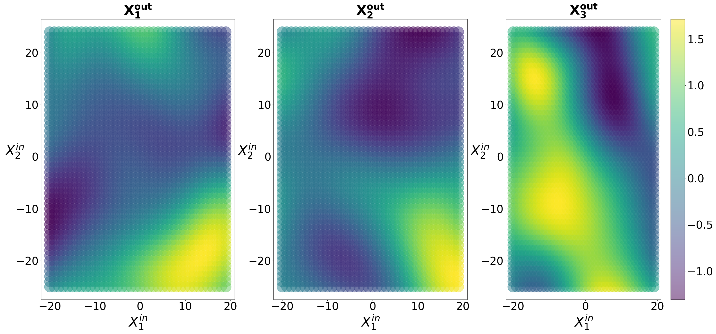
Figure 1. Here we visualize an example of the function $m_{1}$ in (6.2), which is obtained as a single random draw from a zero-mean Gaussian Process mapping $\mathbbm{R}^{3}\to\mathbbm{R}^{3}$. We have plotted its output surface as three scalar functions (left to right) of the first two inputs (the plot axes) with the third input component fixed at 0.

Observe that in the continuous-time framing, changes to $\epsilon$ do not impact the complexity of the learned error term; however, it does grow the magnitude of the error term. In the discrete-time framing, larger values of $\epsilon$ can magnify the complexity of the discrepancy $\Psi_{0}(x)-\Psi^{\dagger}(x)$.

Results

We perform a series of experiments with the L63 system in order to illustrate key points about using data to learn model errors in dynamical systems. First, we demonstrate that hybrid modeling tends to outperform data-only and physics-only methods in terms of prediction quality. We first consider model error as in (6.3); see Figure 2(a) in which we study performance (validity time) versus model error amplitude ($\epsilon$), using random feature maps with $D=200$, and a single trajectory of length $T=100$ sampled at timestep $\Delta t=0.001$. Unless otherwise specified, this is also the configuration used in subsequent experiments.

We see identical trends in Figure 2(b) for a more general case with the non-parametric model error term constructed from Gaussian processes. Interestingly, we see that for small and moderate amounts of model error $\epsilon$, the hybrid methods substantially outperform data-only and physics-only methods. Eventually, for large enough model discrepancy, the hybrid-methods and data-only methods have similar performance; indeed the hybrid-method may be outperformed by the data-only method at large discrepancies. For the simple model error this appears to occur when the discrepancy term is larger in magnitude than $f_{0}$ (e.g. for $b=28$ and $\epsilon=2$, the model error term $\epsilon bu_{x}$ can take on values larger than $f^{\dagger}$ itself).

Figure 2(b) also shows that a continuous-time approach is favored over discrete-time when using data-only methods, but suggests the converse in the hybrid modeling context. We suspect this is an artifact of the different integration schemes used in data generation, training, and testing phases; the data are generated with a higher-fidelity integrator than the one available in training and testing. For the continuous-time method, this presents a fundamental limitation to the forecast quality (we chose this to avoid having artificially high forecast validity times). However, the discrete-time method can overcome this by not only learning the mechanistic model discrepancy, but also the discrepancy term associated with a mis-matched integrator. This typically happens when a closure is perfectly learnable and deterministic (i.e. our Lorenz ’63 example); in this case, the combination of physics-based and integrator-sourced closures can be learned nearly perfectly. In later experiments with a multiscale system, the closures are considered approximate (they model the mean of a noisy underlying process) and the discrete- and continuous-time methods perform more similarly, because the inevitable imperfections of the learned closure term dominate the error rather than the mis-specified integrator. Note that approximate closures driven by scale-separation are much more realistic; thus we should not expect the hybrid discrete-time method to dramatically outperform hybrid continuous-time methods unless other limitations are present (e.g. slow sampling rate).

Importantly, the parameter regime for which hybrid methods sustain advantage over the imperfect physics-only method is substantial; the latter has trajectory predictive performance which drops off rapidly for very small $\epsilon$. This suggests that an apparently uninformative model can be efficiently modified, by machine learning techniques, to obtain a useful model that outperforms a de novo learning approach.

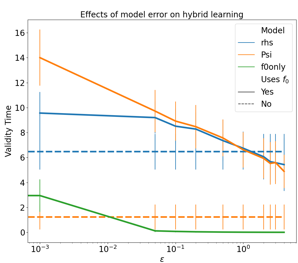
(a)

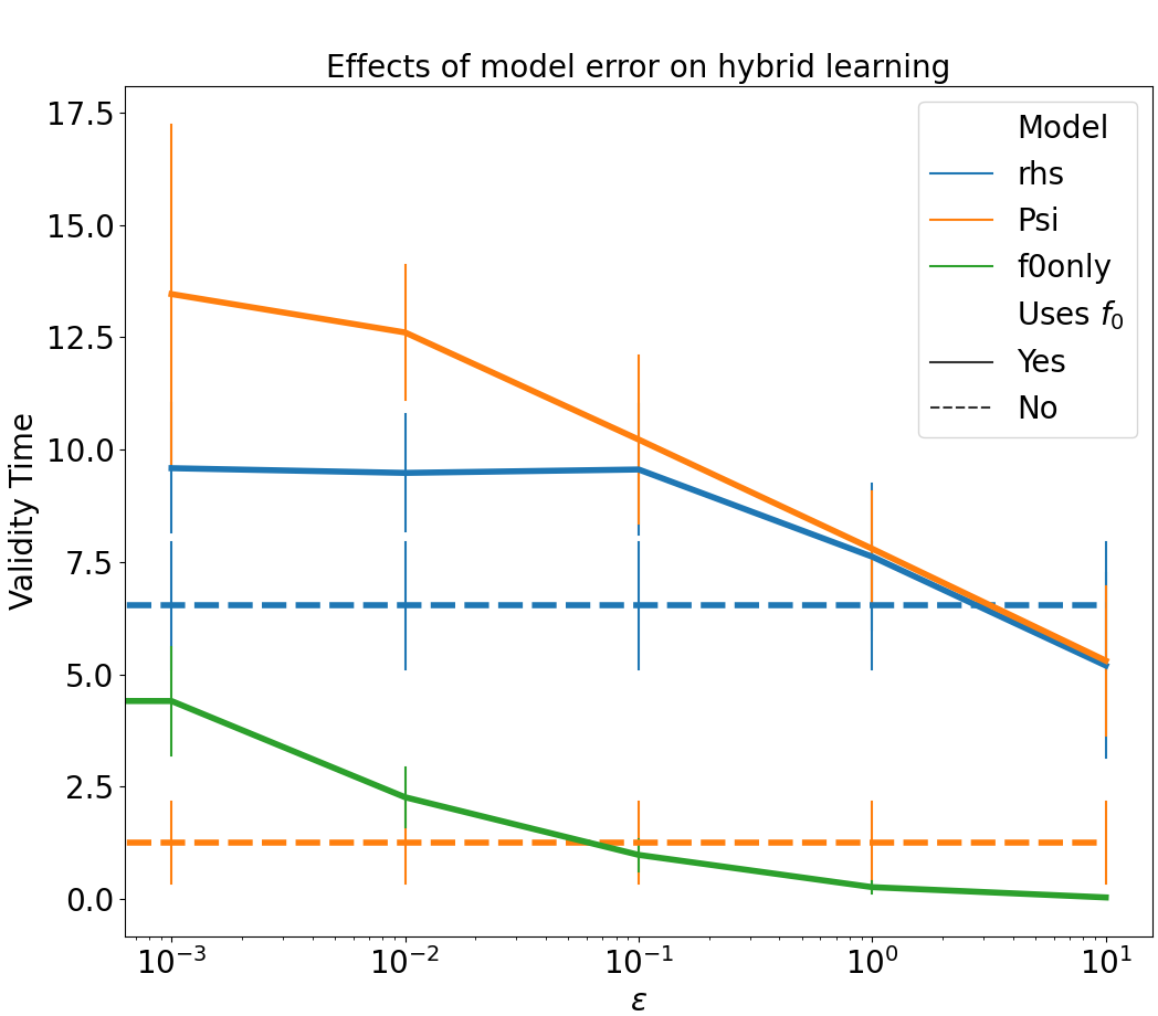
(b)

Figure 2. These plots shows the temporal length of the forecast validity of our learnt models of L63 (6.1), each as a function of model error, as parameterized by $\epsilon$ (6.2) (with $D=200$, $T=100$, and $\Delta t=0.001$). Continuous-time methods are shown in blue, discrete-time approaches in orange. Dotted lines indicate purely data-driven methods to learn the entire vector field defining the dynamics; solid lines indicate methods that learn perturbations to the imperfect mechanistic models $f_{0}$ or $\Psi_{0}$. Integration using the imperfect mechanistic model, without recourse to data, is shown in green. In Figure 2(a), we employ the linear form of model error $m_{1}$ defined in (6.3). In Figure 2(b), we let $m_{1}$ be a single draw from a Gaussian Process, whose structure is shown in Figure 1. Here, we plot means, with error bars as 1 standard deviation.

Next, we show that hybrid methods simplify the machine learning task in terms of complexity of the learned function and, consequently, the amount of data needed for the learning. Figure 3 examines prediction performance (validity time) as a function of training data quantity using random feature maps with $D=2000$ and a fixed parametric model error ($\epsilon=0.2$ in (6.2)) and sampling rate $\Delta t=0.01$. We see that the hybrid methods substantially outperform the data-only approaches in regimes with limited training data. For the continuous-time example, we see an expected trend, where the data-only methods are able to catch up to the hybrid methods with the acquisition of more data. The discrete-time models do not exhibit this behavior, but we expect the data-only discrete-time model to eventually catch up, albeit with additional training data and number of parameters. Note that greater expressivity is also required from data-only methods—our choice of a large $D=2000$ aims to give all methods ample expressivity, and thus test convergence with respect to training data quantity alone. These results demonstrate that the advantage of hybrid modeling is magnified when training data are limited and cannot fully inform de novo learning. Figure 4 further studies the impact of expressivity by again fixing a parametric model error ($\epsilon=0.05$ in (6.2)), training length $T=100$, and sampling rate $\Delta t=0.001$. We see that all methods improve with a larger number of random features, but that relative superiority of hybrid methods is maintained even for $D=10000$.

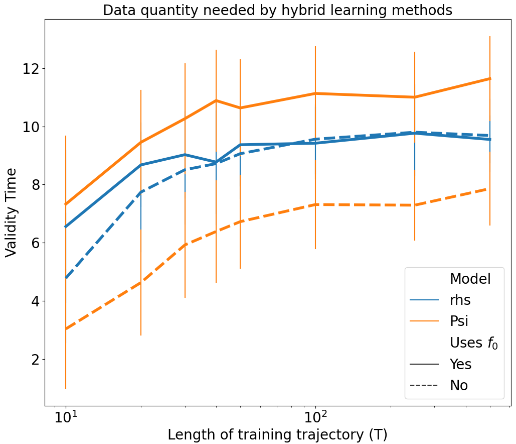
Figure 3. Here we examine the performance of the proposed methods as a function of the length of the interval over which the training data is provided, where $\Delta t=0.01$, ($\epsilon=0.2$ in (6.2)), and $D=2000$ are held constant for the L63 example (6.1). See description of Figure 2 for explanation of legend. We observe that all methods improve with increasing training lengths. We see that, in continuous-time, the primary benefit in hybrid modeling is when the training data are limited.

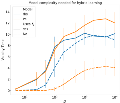
Figure 4. Here we examine the performance of the proposed methods as a function of model complexity, where $\Delta t=0.001$, $\epsilon=0.05$, and $T=100$ are held constant for the L63 example (6.1). See description of Figure 2 for explanation of legend. We observe that all methods improve with increasing number of parameters, and that hybrid methods are especially beneficial when available complexity is limited.

Finally, we study trade-offs between learning in discrete- versus continuous-time for the L63 example (6.1). Figure 5 examines prediction performance (validity time) as a function of data sampling rate $\Delta t$ using random feature maps with $D=200$ with a fixed parametric model error ($\epsilon=0.05$ in (6.2)) and an abundance of training data $T=1000$. We observe that for fast sampling rates ($\Delta t<0.01$), the continuous-time and discrete-time hybrid methods have similar performance. For $\Delta t>0.01$, derivatives become difficult to estimate from the data and the performance of the continuous-time methods rapidly decline. However, the discrete-time methods sustain their predictive performance for slower sampling rates ($\Delta t\in(0.01,0.1)$). At some point, the discrete-time methods deteriorate as well, as the discrete map becomes complex to learn at longer terms because of the sensitivity to initial conditions that is a hallmark of chaotic systems. Here, the discrete-time methods begin to fail around $\Delta t=0.2$; note that they can be extended to longer time intervals by increasing $D$ and amount of training data, but returns diminish quickly.

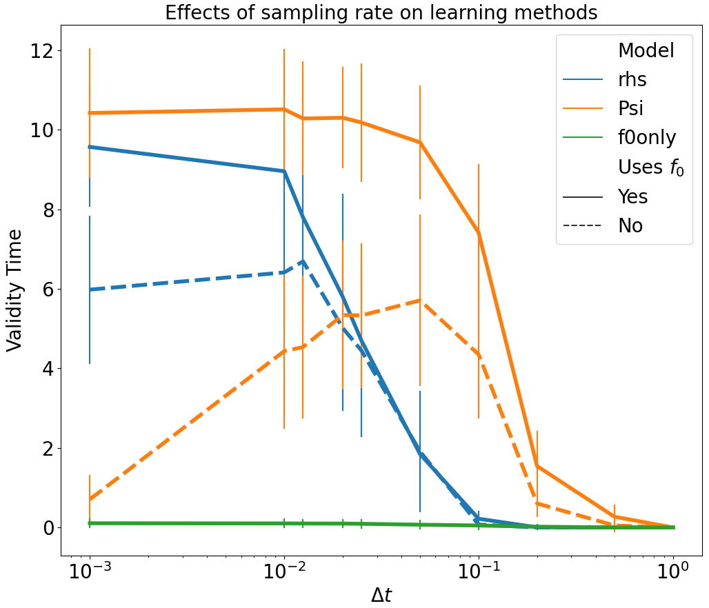
Figure 5. This shows temporal forecast validity as a function of the step size of training data for the tested methods in the L63 example (6.1). We hold fixed $D=200$, $\epsilon=0.05$, and $T=1000$. See description of Figure 2 for explanation of legend. We see that while purely data-driven discrete-time methods struggle at short time steps, the hybrid version thrives in this scenario. All approaches, of course, eventually decay as large time steps create more complex forward maps, due to sensitivity to initial conditions. We also see continuous-time methods work well for small time steps, then deteriorate in tandem with quality of estimated derivatives.

6.2.4. Lorenz ’96 Multiscale (L96MS) System

Setting

Here, we consider the multiscale system [Lorenz, 1996] of form (2.7), where each variable $X_{k}\in\mathbbm{R}$ is coupled to a subgroup of fast variables $Y_{k}\in\mathbbm{R}^{J}$. We have $X\in\mathbbm{R}^{K}$ and $Y\in\mathbbm{R}^{K\times J}$. For $k=1\dots K$ and $j=1\dots J$, we write

(6.4a) $$\dot{X}_{k} =f_{k}(X)+h_{x}\overline{Y}_{k}$$

(6.4b) $$\dot{Y}_{k,j} =\frac{1}{\varepsilon}r_{j}(X_{k},Y_{k})$$

(6.4c) $$\overline{Y}_{k} =\frac{1}{J}\sum_{j=1}^{J}Y_{k,j}$$

(6.4d) $$f_{k}(X) =-X_{k-1}(X_{k-2}-X_{k+1})-X_{k}+F$$

(6.4e) $$r_{j}(X_{k},Y_{k}) =-Y_{k,j+1}(Y_{k,j+2}-Y_{k,j-1})-Y_{k,j}+h_{y}X_{k}$$

(6.4f) $$X_{k+K} =X_{k},\quad Y_{k+K,j}=Y_{k,j},\quad Y_{k,j+J}=Y_{k+1,j}$$

where $\varepsilon>0$ is a scale-separation parameter, $h_{x},h_{y}\in\mathbbm{R}$ govern the couplings between the fast and slow systems, and $F>0$ provides a constant forcing. We set $K=9,\ J=8,\ h_{x}=-0.8,\ h_{y}=1,\ F=10$; this leads to chaotic dynamics for $\varepsilon$ small. When studying scale-separation, we consider $\varepsilon\in\{2^{-7},\ 2^{-5},\ 2^{-3},\ 2^{-1}\}$.

We consider the setting in which we learn Markovian random features models in variable $X$ alone, from $X$ data generated by the coupled $(X,Y)$ system. Large scale-separation between the observed ($X$) and unobserved ($Y$) spaces can simplify the problem of accounting for the unobserved components; in particular, for sufficient scale-separation, we expect a Markovian term to recover a large majority of the residual errors. In fact, we further simplify this problem by learning a scalar-valued model error $M$ that is applied to each $X_{k}$ identically in the slow system:

$$\dot{X}_{k}\approx f_{k}(X)+M(X_{k}).$$

This choice stems from observations about statistical interchangeability amongst the slow variables of the system; these properties of the L96MS model in the scale-separated regime are discussed in [Fatkullin and Vanden-Eijnden, 2004]. We can directly align our reduction of (6.4) with the Markovian hybrid learning framework in (2.2) as follows:

$$\dot{X} \approx f_{0}(X)+m(X)$$

$$f_{0}(X) :=[f_{1}(X),\ \cdots\ ,f_{K}(X)]^{T}$$

$$m(X) :=[M(X_{1}),\ \cdots\ ,M(X_{K})]^{T}.$$

Results

We plot the performance gains of our hybrid learning approaches in Figure 6 by considering validity times of trajectory forecasts, estimation of the invariant measure, and ACF estimation. In all three metrics (and for all scale-separations $\varepsilon$), de novo learning in discrete ($\Psi^{\dagger}\approx m$) and continuous-time ($f^{\dagger}\approx m$) is inferior to using the nominal mechanistic model $f_{0}$. We found that the amount of data used in these experiments is insufficient to learn the full system from scratch. On the other hand, hybrid models in discrete ($\Psi^{\dagger}\approx\Psi_{0}+m$) and continuous-time ($f^{\dagger}\approx f_{0}+m$) noticeably outperformed the nominal physics.

Surprisingly, Figure 6 shows that the Markovian closure methods still qualitatively reproduce the invariant statistics even for large $\varepsilon$ settings where we would expect substantial memory effects. Figure 6 also demonstrates this quantitatively using KL-divergence between invariant measures and mean-squared-error between ACFs. It seems that for this dissipative system, memory effects tend to average out in the invariant statistics. However, the improvements in validity time for trajectory-based forecasting deteriorate for $\varepsilon=2^{-1}$.

To visualize this non-Markovian structure, and how it might be exploited, we examine the residuals from $f_{0}$ in Figure 7 and observe that there are discernible trajectories walking around the Markovian closure term. For small $\varepsilon$, these trajectories oscillate rapidly around the closure term. For large $\varepsilon$ (e.g. $2^{-1}$), however, we observe a slow-moving residual trajectory around the Markovian closure term. This indicates the presence of a stronger memory component, and thus would benefit from a non-Markovian approach to closure modeling.

Jiang and Harlim [2020] show that the memory component in this setting with $\varepsilon=2^{-1}$ can be described using a closure term with a simple delay embedding of the previous state at lag $0.01$. They learn the closure using a kernel method cast in an RKHS framework, for which random feature methods provide an approximation.

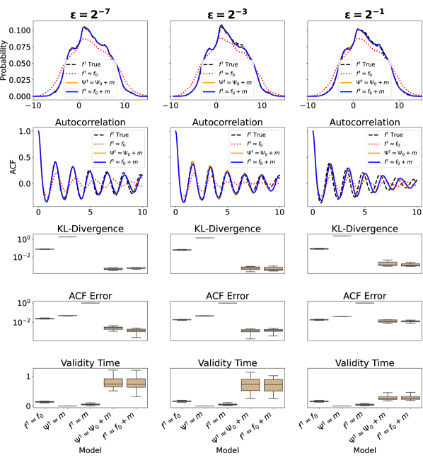
Figure 6. This figure shows the performance of different approaches to modeling the L96MS slow subsystem (6.4). In $f^{\dagger}\approx f_{0}$, we only use the nominal physics $f_{0}$. In $\Psi^{\dagger}\approx m$ and $f^{\dagger}\approx m$, we try to learn the entire right-hand-side using only data (in discrete- and continuous-time settings, respectively). In $\Psi^{\dagger}\approx\Psi_{0}+m$ and $f^{\dagger}\approx f_{0}+m$, we focus on learning Markovian residuals for the known physics (in discrete- and continuous-time settings, respectively). The residual-based correctors substantially outperform the nominal physics and purely data-driven methods according to all presented metrics: invariant measure (shown qualitatively in the first row and quantitatively in the third row), ACF (shown qualitatively in the second row and quantitatively in the fourth row), and trajectory forecasts (shown in the final row). The boxplots show the distributions of quantitative metrics (e.g. KL-divergence, squared errors, validity time), which come from different models, each trained on a different trajectory, and generated using an independent random feature set. Notably, the Markovian residual-based methods’ performance deteriorates for small scale-separation ($\varepsilon=2^{-1}$), where the Markovian assumption breaks down.

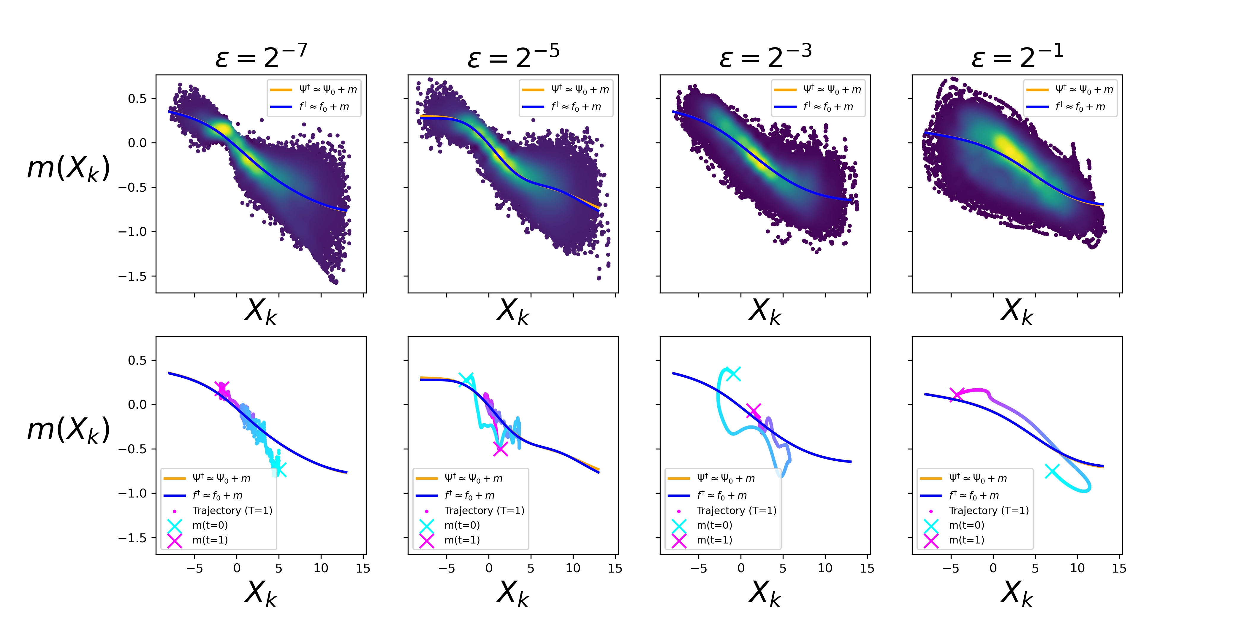
Figure 7. This figure shows the observed and estimated residuals of the nominal physics model $f_{0}$ for the L96MS slow subsystem (6.4) at different scale-separation factors. The first row shows the density of these residuals (yellow is high density, blue is low), as well as the fit of our closure terms in continuous- (blue) and discrete- (orange) time (the discrete model was normalized by dividing by $\Delta t$). The second row shows temporal structure in the errors of our residual fit by superimposing a short (T=1) one-dimensional trajectory (this represents $\sim 0.1\%$ of training data).

6.3. Learning From Partial, Noisy Observations

In this section, we focus on the non-Markovian setting outlined in Section 2.3, and attempt to model the dynamics of the observable using (4.3), with $f_{1}$, $f_{2}$ given by two-layer, fully connected neural networks with GeLU activations [Hendrycks and Gimpel, 2016], and perform the learning by minimizing (4.7) from Section 4.3.3, using 3DVAR for the data assimilation Law et al. [2015, 2013], with the ADAM optimizer [Kingma and Ba, 2015]. The learning rate was initialized at $0.01$ and tuned automatically using a scheduler that halved the learning rate if the training error had not decreased over 10 (mini-batched) epochs. Data were sampled at $\Delta t=0.01$ in all cases, and normalized to have mean zero and unit variance. Numerical integration was performed with the torchdiffeq implementation of the Dormand-Prince adaptive fifth-order Runge-Kutta method: for the L63 example, simple backpropagated autodifferentiation was performed through this solver; for the L96MS example, we used the adjoint method provided by [Rubanova et al., 2019].

6.3.1. Lorenz ’63

We first consider modeling the dynamics of the first-component of the L63 system in (6.1), where we noisily observe the first-component – that is, we observe a noisy trajectory of $u_{x}$ (i.i.d. additive zero-mean, variance-one Gaussian), but do not observe the remaining components $u_{y},u_{z}$. We jointly trained on 100 trajectories, each of length $T=10$ and randomly initialized from a box around the attractor; we chose this approach to ensure that we had data coverage both on and off the attractor although we note that similar success is obtained with a single trajectory of length $T=1000$.). The neural network had width $50.$ We chose an assimilation time of $\tau_{1}=3$ and a forecast time of $\tau_{2}=0.1$. The optimization ran for approximately 200 epochs, and took roughly 24hrs on a single GPU. Adequate results were obtained using a fixed 3DVAR gain matrix $K=[0.5,0,0]^{T}$. However, we present results using the algorithm in which $K=\theta_{\textrm{DA}}$ is jointly learned along with parameters $\theta_{\textrm{DYN}}$, as described in Section 4.3.3; this demonstrates that the gain need not be known a priori.

First, we present results using knowledge that the correct hidden dimension $d_{r}=2$: in Figure 8(a), we show an example of the trained model being assimilated (using 3DVAR with learnt $K$) during the first 3 time units, then predicting for another 7 time units; recall that training was performed using only a $\tau_{2}=0.1$ forecasting horizon, but we evaluate on a longer time horizon to provide a robust test metric. Observe that the learnt hidden dynamics in gray are synchronized with the data, then used to perform the forecast. In Figures 8(b) and 8(c), we show that by solving the system for long time (here, $T=10^{4}$), we are able to accurately reproduce invariant statistics (invariant measure and autocorrelation, resp.) for the true system. In Figure 8(d), we show the evolution of the learnt $K$.

Next, we let $d_{r}=10$, exceeding the true dimension of the hidden states; thus we are able to explore issues caused by learning an overly expressive (in terms of dimension of hidden states) dynamical model. Figure 9 shows dynamics for a learnt model in this setting; we found its reproduction of invariant statistics to be similar to the cases in Figures 8(b) and 8(c), but omit the plots for brevity. This success aligns with the approximation theory, as discussed in Remark 5.5, and provides empirical reassurance that the methodology can behave well in situations where the dimension of the hidden variable is unknown and dimension $d_{r}$ used in learning exceeds its true dimension. Nevertheless, we construct an example in Section 6.4 in which a specific embedding of the true dynamics in a system of higher dimension can lead to poor approximation; this is caused by an instability in the model which allows departure from the invariant manifold on which the true dynamics is accurately captured. However, we emphasize that this phenomenon is not observed empirically in the experiment reported here with $d_{r}=10.$ Nonetheless we also note expected decreases in efficiency caused by over-estimating the dimension of the hidden variable, during both model training and testing; thus determining the smallest choice for $d_{r}$, compatible with good approximation, is important. Recent research has addressed this challenge in the discrete-time setting by applying manifold learning to a delay-embedding space, then using the learnt manifold to inform initialization and dimensionality of LSTM hidden states [Kemeth et al., 2021].

Note that our early attempts at achieving these numerical results, using the optimization ideas in Sections 4.3.1 and 4.3.2, yielded unstable models that exhibited blow-up on shorter time scales (e.g. $T<1000$); however, by incorporating data assimilation as in Chen et al. [2021b], and further tuning the optimization to achieve lower training errors, we were able to obtain a model that, empirically, did not exhibit blow-up, even when solved for very long time (e.g. $T=10^{5}$). We also note that we were unable to achieve such high-fidelity results using the methods of [Ouala et al., 2020] on neural networks with non-linear activation functions; this may be explained by noting that Ouala et al. [2020] achieved their results using linear, identity-based activations, resulting in inference of polynomial models containing the true L63 model.

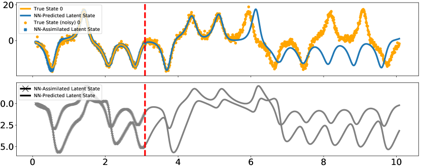
(a)

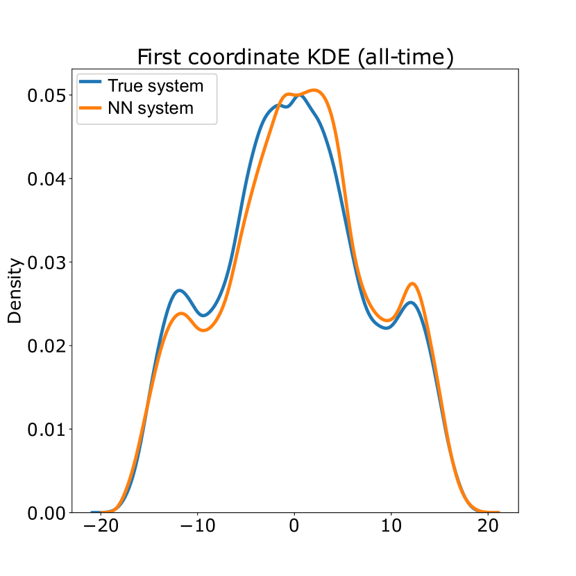
(b)

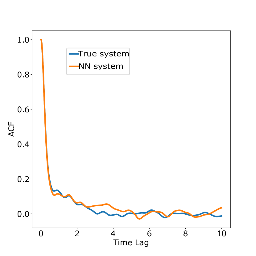
(c)

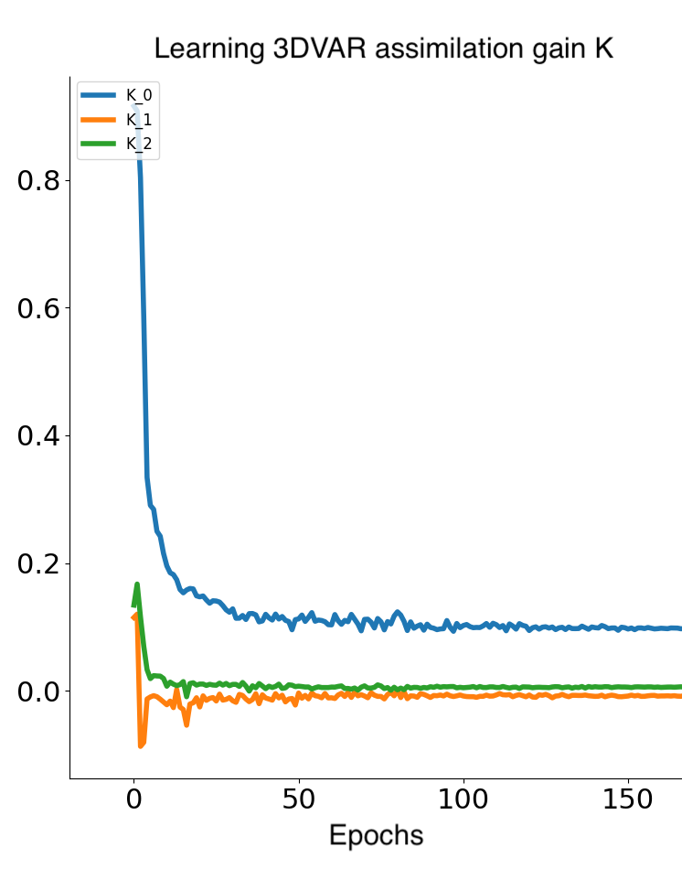
(d)

Figure 8. This figure concerns learning of a continuous-time RNN to model the L63 system (6.1), based on noisy observation of only the first component; it uses an augmented state space $d_{r}=2$. Figure 8(a) shows how the trained model can be used for forecasting—by first synchronizing to data using 3DVAR, then forecasting into the future. The top-half depicts dynamics of the observed component (model-solutions in blue; observations in yellow); the bottom-half depicts the augmented state space (both hidden components are shown in gray). We observed a validity time of roughly 3 model time units. Figures 8(b) and 8(c) shows that long-time solutions of the learnt model accurately mirror invariant statistics (invariant measure and autocorrelation, resp.) for the true system. Figure 8(d) shows the learning process for estimating a 3DVAR gain $K$.

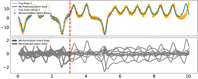
Figure 9. This figure concerns learning of a continuous-time RNN to model the L63 system (6.1), based on noisy observation of only the first component; it uses an augmented state space $d_{r}=10$. The top-half depicts dynamics of the observed component (model-solutions in blue; observations in yellow); the bottom-half depicts the augmented state space (all 10 hidden components are shown in gray). In the first 3 time units, the model is assimilated to a sequence of observed data using 3DVAR, then in the subsequent 7 time units, a forecast is issued. We found this model to have similar short-term and long-term fidelity when compared to the model presented in Figures 8(a), 8(b), 8(c) and 8(d), which used the correct hidden dimension $d_{r}=2$.

6.3.2. Lorenz ’96 Multiscale ($\varepsilon=2^{-1}$)

Recall that Markovian closures fail to capture autocorrelation statistics for the slow components of this model in the case of $\varepsilon=2^{-1}$ (see top right panel of LABEL:fig:l96acf). As evidenced by the slow-moving trajectory around the Markovian closure in Figure 7, this is a case ripe for non-Markovian modeling. We investigate the applicability of our continuous-time ODE formulation in (4.3), using a neural network of width of $1000$. We applied the above described methodology for minimizing (4.7), under the data setting described in Section 6.2.4, to learn hidden dynamics. Similarly to the previous section, we jointly trained on 100 trajectories, each of length $T=20$ and randomly initialized from a box around the attractor. We chose an assimilation time of $\tau_{1}=2$ and a forecast time of $\tau_{2}=1$; note that longer times can become quite costly, especially for high-dimensional systems; nevertheless, the assimilation time $\tau_{1}$ appears intrinsically tied to the amount of memory present in the system.

In Figures 10(a) and 10(b), we plot comparisons of the true and learnt (via (4.3)) ACF and invariant measure, and observe substantial improvement over the Markovian closure. However, this learnt model exhibited instabilities when solved for longer than $T=500$. We expect that this can be remedied via further training (as was found for the L63 example); however, the incorporation of stability constraints into the model, as in Schneider et al. [2021], would be valuable. In order to train this larger model for longer time, further studies of efficient optimization must also be performed in this setting ([Chen et al., 2021b] has begun highly relevant investigation in this direction).

In Figure 11, we visualize the learnt 3DVAR gain (which encodes the learnt model’s covariance structure), in which each row corresponds to the gain for a given component of the learnt model as a function of observed components (indexed in the columns); trends are elucidated via hierarchical clustering and a row-based normalization of the learnt matrix $K$. It clearly learns a consistent diagonal covariance structure for the observables. More impressively, it illustrates cross-covariances between observed and hidden components that mirror the compartmentalized structure of the model in (6.4); note that each observed component has a distinct grouping of hidden variables which have high correlation (white) primarily with that component and low correlation (black) with other observables. This type of analysis may provide greater interpretability of learnt models of hidden dynamics.

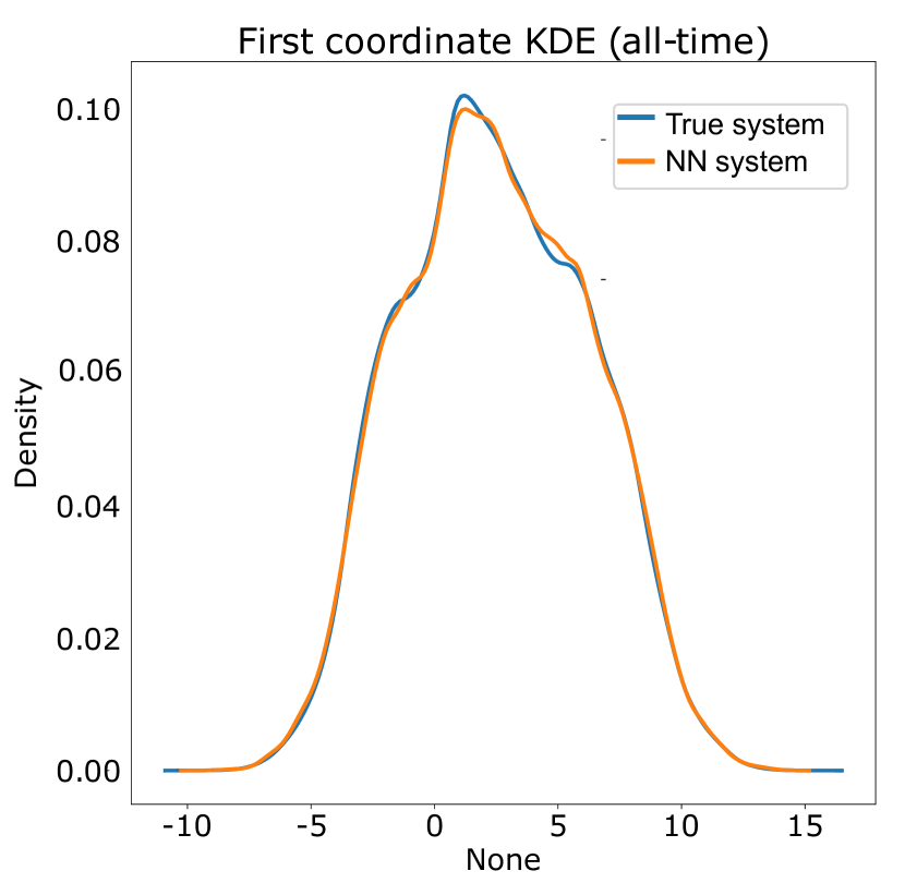
(a)

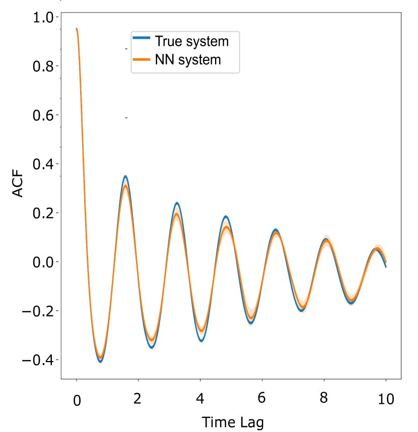
(b)

Figure 10. This figure concerns learning of a continuous-time RNN to model the first 9 (slow) components of the L96MS system ($\varepsilon=0.5$ in (6.4)), based on noisy observations of these slow components; it uses an augmented state space $d_{r}=72$. We trained using noised observations (standard deviation $0.01$) of only the first 9 components of the true $81-$dimensional system. These plots show that this model can accurately reproduce both the invariant measure (Figure 10(a)) and ACF (Figure 10(b)) for these observed states. These statistics were calculated by running the learnt model for $T=500$ model time units; longer runs encountered instabilities that caused trajectories to leave the attractor and blow-up.

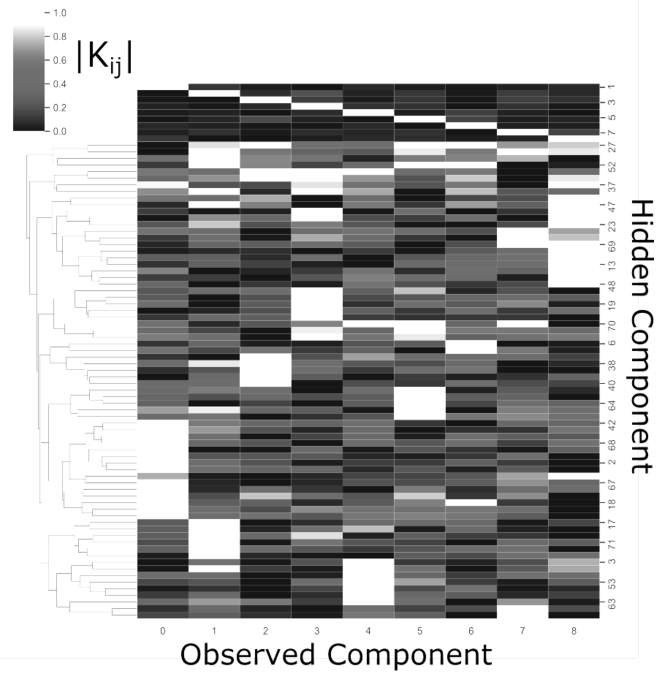
Figure 11. Here we visualize the learnt 3DVAR gain matrix $K$ (81 x 9) ($\theta_{\textrm{DA}}$ in Section 4.3.3) associated with the non-Markovian learning of L96MS (6.4). We first compute entry-wise absolute values, then apply a row-normalization; white indicates highest correlation, and black indicates lowest correlation. The top 9 rows shown directly correspond to the first 9 rows of $K$. The bottom 72 rows are re-ordered (via hierarchical clustering) to illustrate associations between the 9 observed components and the 72 hidden variables.

6.4. Initializing and Stabilizing the RNN

As mentioned in Remark 5.8 the RNN approximates an enlarged system which contains solutions of the original system as trajectories confined to the invariant manifold $m=m^{\dagger}(x,y)$; see identity (5.14). However, this invariant manifold may be unstable, either as a manifold within the continuous-time model (5.13), or as a result of numerical instability. We now demonstrate this with numerical experiments. This instability points to the need for data assimilation to be used with RNNs if prediction of the original system is desired, not only to initialize the system but also to stabilize the dynamics to remain near to the desired invariant manifold.

To illustrate these challenges, we consider the problem of modeling evolution of a single component of the L63 system (6.1). Consider this as variable $x$ in (2.7). As exhibited in (5.13), model error may be addressed in this setting by learning a representation that contains the hidden states $y$ in (2.7) (i.e. the other two unobserved components of (6.1)), but since the dimension of the hidden states is typically not known a priori the dimensions of the latent variables in the RNN (and the system it approximates) may be greater than those of $y$; in the specific construction we use to prove the existence of an approximating RNN we introduce a vector field for evolution of the error $m$ as well as $y$. We now discuss the implications of embedding the true dynamics in a higher dimensional system in the specific context of the embedded system (5.13). However the observations apply to any embedding of the desired dynamics (2.7) (with $\epsilon=1$) within any higher dimensional system.

We choose examples for which (5.14) implies that $m-m^{\dagger}$ is constant in time. Then, under (5.13),

$$\bigl{(}m-m^{\dagger}(x,y)\bigr{)}(t)={\rm constant};$$

that is, it is constant in time. The desired invariant manifold (where the constant is $0$) is thus stable. However this stability only holds in a neutral sense: linearization about the manifold exhibits a zero eigenvalue related to translation of $m-m^{\dagger}$ by a constant. We now illustrate that this embedded invariant manifold can be unstable; in this case the instability is caused by numerical integration, which breaks the conservation of $m-m^{\dagger}$ in time.

Example 1: Consider equation (6.1) which we write in form (2.8) by setting $x=u_{x}$ and $y=(u_{y},u_{z}).$ Then we let $f_{0}(u_{x}):=-au_{x}$ yielding $m^{\dagger}(u_{y})=au_{y}$. Thus $f^{\dagger}=f_{0}+m^{\dagger}$ is defined by the first component of the right-hand side of (6.1). The function $g^{\dagger}(u_{y},u_{z})$ is then given by the second and third components of the right-hand side of (6.1). Applying the methodology leading to (5.13) to (6.1) results in the following four dimensional system:

(6.5a) $$\dot{u}_{x} =f_{0}(u_{x})+m, u_{x}(0) =x_{0},$$

(6.5b) $$\dot{u}_{y} =bu_{x}-u_{y}-u_{x}u_{z}, u_{y}(0) =y_{0},$$

(6.5c) $$\dot{u}_{z} =-cu_{z}+u_{x}u_{y}, u_{z}(0) =z_{0},$$

(6.5d) $$\dot{m} =a\bigl{(}bu_{x}-u_{y}-u_{x}u_{z}\bigr{)}, m(0) =m^{\dagger}(y_{0}).$$

Here we have omitted the $u_{y}$-dependence from the equation (6.1) for $u_{x}$, and aim to learn this error term; we introduce the variable $m$ in order to do so. This system, when projected into $u_{x},u_{y},u_{z}$, behaves identically to (6.1) when $m(0)=m^{\dagger}(y_{0})$. Thus the $4-$dimensional system in (6.5) has an embedded invariant manifold on which the dynamics is coincident with that of the $3-$dimensional L63 system.

We numerically integrate the $4-$dimensional system in (6.5) for 10000 model time units (initialized at $x_{0}=1,y_{0}=3,z_{0}=1,m_{0}=ay_{0}=30$), and show in Figure 12 that the resulting measure for $u_{x}$ (dashed red) is nearly identical to its invariant measure in the traditional $3-$dimensional L63 system in (6.1) (solid black). However, we re-run the simulation for a perturbed $m(0)=m^{\dagger}(y_{0})+1$, and see in Figure 12 (dotted blue) that this yields a different invariant measure for $u_{x}$. This result emphasizes the importance of correctly initializing an RNN not only for efficient trajectory forecasting, but also for accurate statistical representation of long-time behavior.

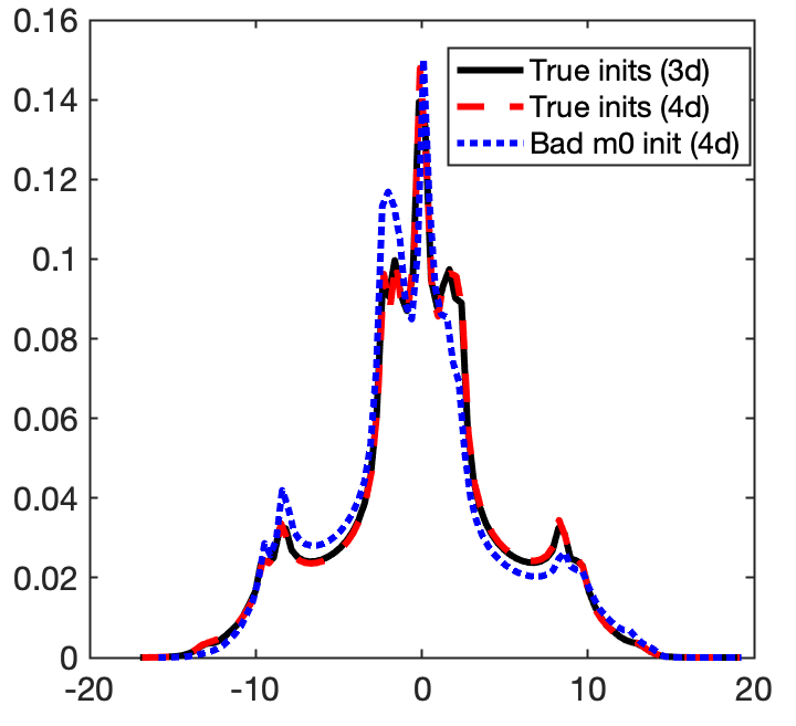
Figure 12. Here, we show that the invariant density for the first component of L63 (black) can be reproduced by a correctly initialized augmented $4-$d system (dashed red) in (6.5). However, incorrect initialization of $m(0)$ in (6.5) (dotted blue) yields a different invariant density.

Example 2: Now we consider (6.1) which we write in form (2.8) by setting $x=u_{z}$ and $y=(u_{x},u_{y}).$ We let $f_{0}(u_{z}):=-cu_{z}$ and $m^{\dagger}(u_{x},u_{y}):=u_{x}u_{y}$, so that $f^{\dagger}=f_{0}+m^{\dagger}$ corresponds to the third component of the right-hand side of (6.1). Function $g^{\dagger}(u_{x},u_{y})$ is defined by the first two components of the right-hand side of (6.1). We again form a $4-$dimensional system corresponding to (6.1) using the methodology that leads to (5.13):

(6.6a) $$\dot{u}_{x} =a(u_{y}-u_{x}), u_{x}(0) =x_{0},$$

(6.6b) $$\dot{u}_{y} =bu_{x}-u_{y}-u_{x}u_{z}, u_{y}(0) =y_{0},$$

(6.6c) $$\dot{u}_{z} =f_{0}(u_{z})+m, u_{z}(0) =z_{0},$$

(6.6d) $$\dot{m} =u_{x}\dot{u}_{y}+u_{y}\dot{u}_{x}, m(0) =m^{\dagger}(x_{0},y_{0}).$$

We integrate (6.6) for 3000 model time units (initialized at $x_{0}=1,y_{0}=3,z_{0}=1,m_{0}=x_{0}y_{0}=3$), and show in Figure 13 that the $3-$dimensional Lorenz attractor is unstable with respect to perturbations in the numerical integration of the $4-$dimensional system. The solutions for $u_{x},u_{y},u_{z}$ eventually collapse to a fixed point after the growing discrepancy between $m(t)$ and $m^{\dagger}$ becomes too large. The time at which collapse occurs may be delayed by using smaller tolerances within the numerical integrator (we employ Matlab rk45) demonstrating that the instability is caused by the numerical integrator. This collapse is very undesirable if prediction of long-time statistics is a desirable goal. On the other hand, Figure 14 shows short-term accuracy of the $4-$dimensional system in (6.6) up to 12 model time units when correctly initialized ($m_{0}=m^{\dagger}(x_{0},y_{0})$, dashed red), and accuracy up to 8 model time units when initialization of $m_{0}$ is perturbed ($m_{0}=m^{\dagger}(x_{0},y_{0})+1$, dotted blue). This result demonstrates the fundamental challenges of representing chaotic attractors in enlarged dimensions and may help explain observations of RNNs yielding good short-term accuracy, but inaccurate long-term statistical behavior. While empirical stability has been observed in some discrete-time LSTMs [Vlachas et al., 2020, Harlim et al., 2021], the general problem illustrated above is likely to manifest in any problems where the dimension of the learned model exceeds that of the true model; the issue of how to address initialization of such models, and its interaction with data assimilation, therefore merits further study.

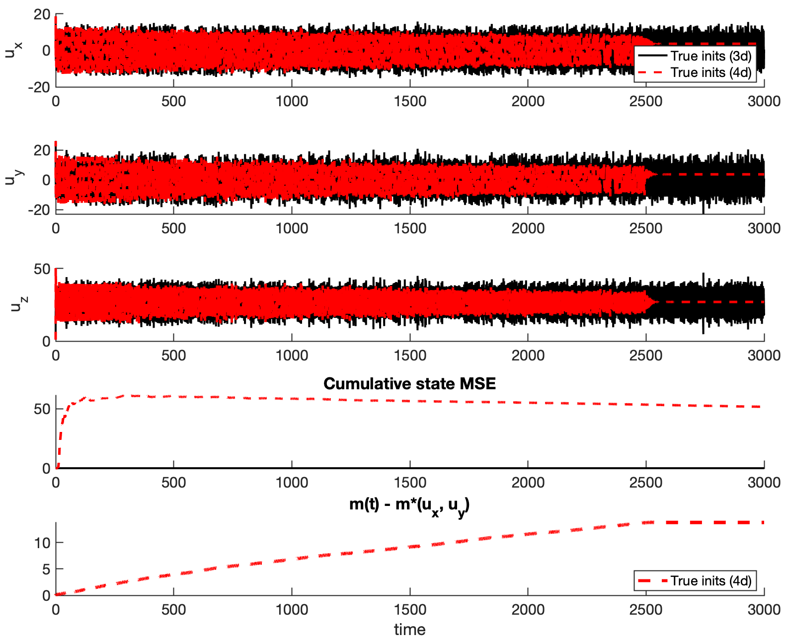
Figure 13. Here we show that the embedded $3-$dimensional manifold of L63, within the $4-$dimensional system given by (6.6), is unstable. Indeed the correctly initialized $4-$dimensional system (dashed red) has solution which decays to a fixed point. The bottom figure shows divergence of the numerically integrated model error term $m(t)$ and the state-dependent term $m^{\dagger}$; this growing discrepancy is likely responsible for the eventual collapse of the $4-$dimensional system.

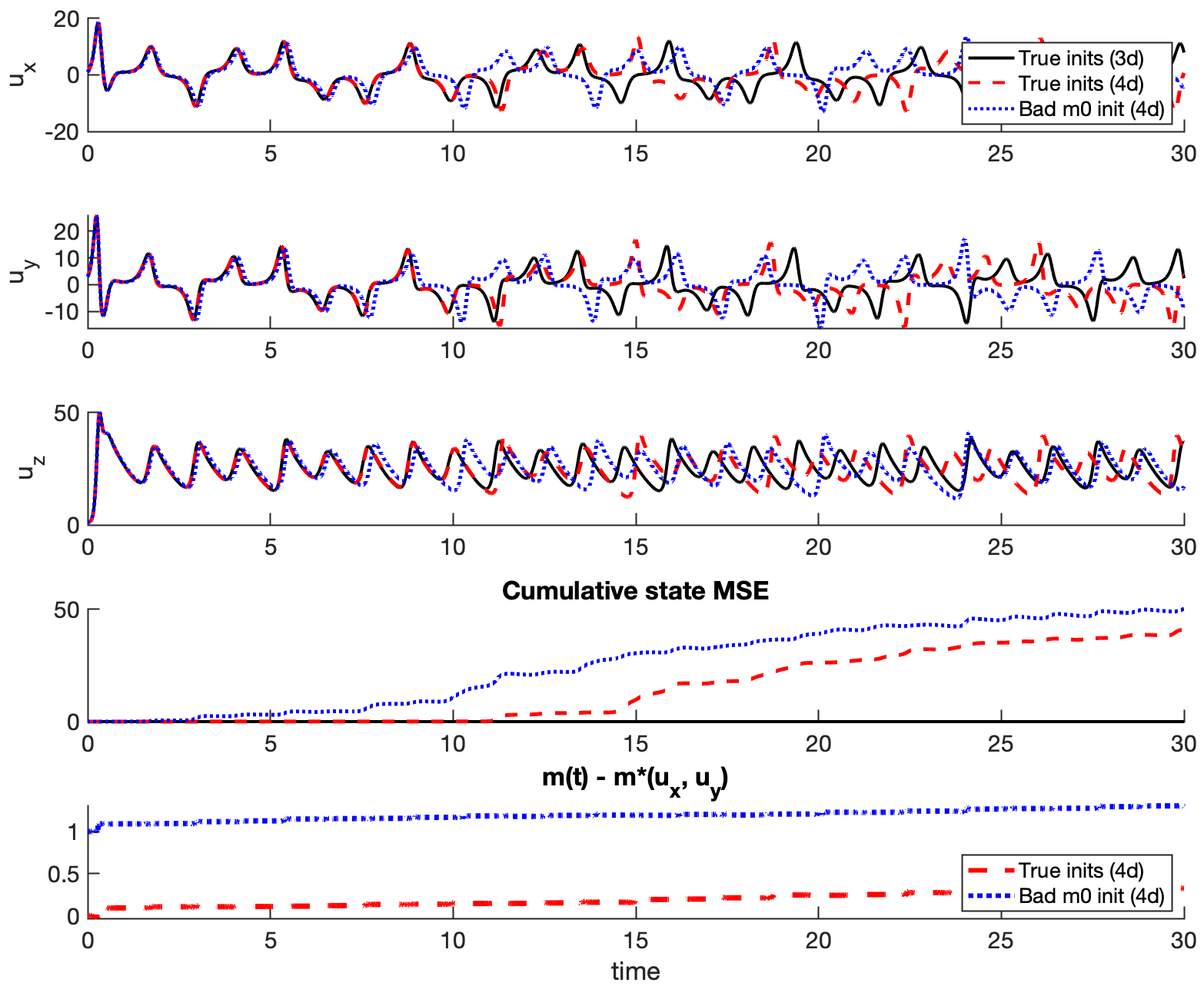
Figure 14. Here, we show short-term accuracy for the $4-$dimensional system in (6.6). Predictions using the correct initialization of $m_{0}$ (dashed red) remain accurate for nearly twice as long as predictions that use a perturbed initialization ($m_{0}=m^{\dagger}(u_{x},u_{y})+1$). The bottom figure shows that $m(t)$ diverges from the state-dependent $m^{\dagger}$ more quickly for the poorly initialized model, but in both cases errors accumulate over time.

7. Conclusions

In this work we evaluate the utility of blending mechanistic models of dynamical systems with data-driven methods, demonstrating the power of hybrid approaches. We provide a mathematical framework that is consistent across parametric and non-parametric models, encompasses both continuous- and discrete-time, and allows for Markovian and memory-dependent model error. We also provide basic theoretical results that underpin the adopted approaches. The unified framework elucidates commonalities between seemingly disparate approaches across various applied and theoretical disciplines. It would be desirable if the growing recognition of the need for hybrid modeling were to motivate flexible incorporation of mechanistic models into open-source software for continuous-time Markovian and non-Markovian modeling of error [Ouala et al., 2020, Rubanova et al., 2019, Chang et al., 2019, Erichson et al., 2020, Anantharaman et al., 2020, Gupta and Lermusiaux, 2021].

Our work is focused on immutable mechanistic models ($f_{0}$ and $\Psi_{0}$), but these models themselves often have tunable parameters. In principle one can jointly learn parameters for the mechanistic model and closure term. However, the lack of identifiability between modifying the closure and modifying the physics brings up an interesting question in explainability. Future work might focus on decoupling the learning of parameters and closure terms so that maximal expressivity is first squeezed out of the mechanistic model [Plumlee and Joseph, 2017, Plumlee, 2017].

Our numerical results demonstrate the superiority of hybrid modeling over learning an entire system from scratch, even when the available mechanistic model has large infidelities. Hybrid modeling also showed surprisingly large performance gains over using mechanistic models with only small infidelities. We quantify these improvements in terms of data hunger, demands for model complexity, and overall predictive performance, and find that all three are significantly improved by hybrid methods in our experiments.

We establish bounds on the excess risk and generalization error that decay as $1/\sqrt{T}$ when learning model discrepancy from a trajectory of length $T$ in an ergodic continuous-time Markovian setting. We make minimal assumptions about the nominal physics (i.e. $f_{0}\in C^{1}$); thus, our result equivalently holds for learning the entire vector field $f^{\dagger}$ (i.e $f_{0}\equiv 0$). However the upper bounds on excess risk and generalization error scale with the size of the function being learned, hence going some way towards explaining the superiority of hybrid modeling observed in the numerical experiments. Future theoretical work aimed at quantifying the benefits of hybrid learning versus purely data-driven learning is of interest. We also note that the ergodic assumption underlying our theory will not be satisfied by many dynamical models, and alternate statistical learning theories need to be developed in such settings.

We illustrate trade-offs between discrete-time and continuous-time modeling approaches by studying their performance as a function of training data sample rate. We find that hybrid discrete-time approaches can alleviate instabilities seen in purely data-driven discrete-time models at small timesteps; this is likely due to structure in the integrator $\Psi_{0}$, which has the correct parametric dependence on timestep. In the continuous-time setting, we find that performance is best when derivatives can accurately be reconstructed from the data, and deteriorates in tandem with differentiation inaccuracies (caused by large timesteps); continuous-time hybrid methods appear to offer additional robustness to inaccurate differentiation when compared to purely data-driven methods. In cases of large timesteps and poorly resolved derivatives, ensemble-based data assimilation methods may still allow for accurate learning of residuals to the flow field for continuous-time modeling [Gottwald and Reich, 2021b].

Finally, we study non-Markovian memory-dependent model error, through numerical experiments and theory, using RNNs. We prove universal approximation for continuous-time hybrid RNNs and demonstrate successful deployment of the methodology. Future work focusing on the effective training of these models, for more complex problems, would be of great value; ideas from data assimilation are likely to play a central role Chen et al. [2021b]. Further work on theoretical properties of reservoir computing (RC) variants on RNNs would also be of value: they benefit from convex optimization, and may be viewed as random feature methods between Banach spaces. These RNN and RC methods will benefit from constraining the learning to ensure stability of the latent dynamical model. These issues are illustrated via numerical experiments that relate RNNs to the question of stability of invariant manifolds representing embedded desired dynamics within a higher dimensional system.

8. Appendix

8.1. Proof of Excess Risk/Generalization Error Theorem

Note that in both (5.7) and (5.8) $\varphi(\cdot)$ is only evaluated on (compact) $\mathcal{A}$ obviating the need for any boundedness assumptions on the functions $\{f_{\ell}\}_{\ell=0}^{p}$ and $m^{\dagger}$ in what follows.

Lemma 8.1.

Let Assumptions A1 and A2 hold. Then there is $\Sigma$ positive semi-definite symmetric in $\mathbb{R}^{p\times p}$ such that $\theta^{\ast}_{T}\to\theta^{\ast}_{\infty}$ almost surely, and $\sqrt{T}(\theta^{\ast}_{T}-\theta^{\ast}_{\infty})\Rightarrow N(0,\Sigma)$ with respect to $x(0)\sim\mu.$ Furthermore, there is constant $C\in(0,\infty)$ such that, almost surely w.r.t. $x(0)\sim\mu$,

$${\rm limsup}_{T\to\infty}\Bigl{(}\frac{T}{\log\log T}\Bigr{)}^{\frac{1}{2}}\|\theta^{\ast}_{T}-\theta^{\ast}_{\infty}\|\leq C.$$

Proof.

By rearranging the equation for $\theta^{\ast}_{\infty}$ we see that

$$A_{\scriptsize{T}}\theta^{\ast}_{T} =b_{\scriptsize{T}},$$

$$A_{\scriptsize{T}}\theta^{\ast}_{\infty} =b_{\infty}+(A_{\scriptsize{T}}-A_{\infty})\theta^{\ast}_{\infty}.$$

Thus, subtracting,

(8.1) $$(\theta^{\ast}_{T}-\theta^{\ast}_{\infty})=A_{\scriptsize{T}}^{-1}(b_{\scriptsize{T}}-b_{\infty})-A_{\scriptsize{T}}^{-1}(A_{\scriptsize{T}}-A_{\infty})\theta^{\ast}_{\infty}.$$

Because $\{f_{\ell}(\cdot)\}$ and $m^{{\dagger}}(\cdot)$ are Hölder (Assumption A2, and discussion immediately preceding it), so are $\bigl{\langle}f_{i}(\cdot),f_{j}(\cdot)\bigr{\rangle}$ and $\bigl{\langle}m^{{\dagger}}(\cdot),f_{j}(\cdot)\bigr{\rangle}.$ Thus each entry of matrix $A_{\scriptsize{T}}$ (resp. vector $b_{\scriptsize{T}}$) converges almost surely to its corresponding entry in $A_{\infty}$ (resp. $b_{\infty}$), by the ergodicity implied by Assumption A1, and the pointwise ergodic theorem. The almost sure convergence of $\theta^{\ast}_{T}$ to $\theta^{\ast}_{\infty}$ follows, after noting that $A_{\infty}$ is invertible. Furthermore, also by Assumption A1, there are constants $\{\sigma_{ij}\},\{\sigma_{j}\}$ such that

$$\sqrt{T}\Bigl{(}(A_{\scriptsize{T}})_{ij}-(A_{\infty})_{ij}\Bigr{)}\Rightarrow N(0,\sigma_{ij}^{2}),$$

$$\sqrt{T}\Bigl{(}(b_{\scriptsize{T}})_{j}-(b_{\infty})_{j}\Bigr{)}\Rightarrow N(0,\sigma_{j}^{2}).$$

Since arbitrary linear combinations of the $\{(A_{\scriptsize{T}})_{ij}\},\{(b_{\scriptsize{T}})_{j}\}$ are time-averages of Hölder functions, it follows that $\sqrt{T}\{A_{\scriptsize{T}}-A_{\infty},b_{\scriptsize{T}}-b_{\infty}\}$ converges in distribution to a Gaussian, by the Cramér-Wold Theorem [Grimmett and Stirzaker, 2020]. Weak convergence of $\sqrt{T}(\theta^{\ast}_{T}-\theta^{\ast}_{\infty})$ to a Gaussian follows from (8.1) by use of the Slutsky Lemma [Grimmett and Stirzaker, 2020], since $A_{T}$ converges almost surely to invertible $A_{\infty}.$ Matrix $\Sigma$ cannot be identified explicitly in terms of only the $\{\sigma_{ij}\},\{\sigma_{i}\}$ because of correlations between $A_{T}$ and $b_{T}$. The almost sure bound on $\|\theta^{\ast}_{T}-\theta^{\ast}_{\infty}\|$ follows from (8.1) after multiplying by $(T/\log\log T)^{\frac{1}{2}}$, noting that $A_{\scriptsize{T}}\to A_{\infty}$ almost surely, and the almost sure bounds on $(T/\log\log T)^{\frac{1}{2}}\{\|A_{\scriptsize{T}}-A_{\infty}\|,\|b_{\scriptsize{T}}-b_{\infty}\|\}$, using Assumption A1. ∎

In what follows it is helpful to define

$$R_{T}^{+} =(\theta^{\ast}_{T}-\theta^{\ast}_{\infty})\bigl{(}\|\theta^{\ast}_{T}\|+\|\theta^{\ast}_{\infty}\|+1\bigr{)},$$

$$G_{T}^{+} =\mathcal{I}_{T}(m^{\ast}_{\infty})-\mathcal{I}_{\infty}(m^{\ast}_{\infty}).$$

Lemma 8.2.

Let Assumption A2 hold. Then, assuming $x(0)\sim\mu$, there is constant $C>0$ such that the excess risk $R_{T}$ satisfies

$$R_{T}\leq C\|R_{T}^{+}\|.$$

Furthermore the generalization error satisfies

$$|G_{T}|\leq 2C\|R_{T}^{+}\|+|G_{T}^{+}|.$$

Proof.

For the bound on the excess risk we note that

$$R_{T} =\mathcal{L}_{\mu}(m^{\ast}_{T},m^{\dagger})-\mathcal{L}_{\mu}(m^{\ast}_{\infty},m^{\dagger})$$

$$=\int_{\mathbbm{R}^{d_{x}}}\Bigl{\langle}(m^{\ast}_{T}-m^{\ast}_{\infty})(x),(m^{\ast}_{T}+m^{\ast}_{\infty}-2m^{\dagger})(x)\Bigr{\rangle}\,\mu(dx)$$

$$\leq\Bigl{(}\int_{\mathbbm{R}^{d_{x}}}\bigl{\|}(m^{\ast}_{T}-m^{\ast}_{\infty})(x)\bigr{\|}^{2}\,\mu(dx)\Bigr{)}^{\frac{1}{2}}\Bigl{(}\int_{\mathbbm{R}^{d_{x}}}\bigl{\|}(m^{\ast}_{T}+m^{\ast}_{\infty}-2m^{\dagger})(x)\bigr{\|}^{2}\,\mu(dx)\Bigr{)}^{\frac{1}{2}}.$$

The first follows from the boundedness of the $\{f_{\ell}\}_{\ell=1}^{p}$ and $m^{\dagger}$, since the first term in the product above is bounded by a constant multiple of $\|\theta^{\ast}_{T}-\theta^{\ast}_{\infty}\|$ and the second term by a constant multiple of $\|\theta^{\ast}_{T}\|+\|\theta^{\ast}_{\infty}\|+\sup_{\mathcal{A}}\|m^{\dagger}\|.$

For the bound on the generalization error we note that

$$G_{T} =\mathcal{I}_{T}(m^{\ast}_{T})-\mathcal{I}_{\infty}(m^{\ast}_{T})$$

$$=\mathcal{I}_{T}(m^{\ast}_{T})-\mathcal{I}_{T}(m^{\ast}_{\infty})$$

$$\quad\quad\quad\quad\quad+\mathcal{I}_{T}(m^{\ast}_{\infty})-\mathcal{I}_{\infty}(m^{\ast}_{\infty})$$

$$\quad\quad\quad\quad\quad\quad\quad\quad\quad\ \ \ +\mathcal{I}_{\infty}(m^{\ast}_{\infty})-\mathcal{I}_{\infty}(m^{\ast}_{T})$$

$$=\bigl{(}\mathcal{I}_{T}(m^{\ast}_{T})-\mathcal{I}_{T}(m^{\ast}_{\infty})\bigr{)}+G_{T}^{+}-R_{T}.$$

The third term in the final identity is the excess risk that we have just bounded; the first term may be bounded in the same manner that we bounded the excess risk, noting that integration with respect to $\mu$ is simply replaced by integration with respect to the empirical measure generated by the trajectory data which, by assumption, is confined to the attractor $\mathcal{A}$; the second term is simply $G_{T}^{+}.$ Thus the result follows. ∎

Proof of Theorem 5.2.

By Assumption A1, with choice of $\varphi(x)=\|m^{\dagger}(x)-m^{\ast}_{\infty}(x)\|^{2},$ $\sqrt{T}G_{T}^{+}$ converges in distribution to a scalar-valued centred Gaussian. By Lemma 8.1 and the Slutsky Lemma [Grimmett and Stirzaker, 2020], $\sqrt{T}R_{T}^{+}$ converges in distribution to a centred Gaussian in $\mathbb{R}^{p}.$ By the Cramer-Wold Theorem [Grimmett and Stirzaker, 2020] $\sqrt{T}(R_{T}^{+},G_{T}^{+})$ converges in distribution to a centred Gaussian in $\mathbb{R}^{p+1}.$

The convergence in distribution results for excess risk $R_{T}$ and generalization error $|G_{T}|$ then follow from Lemma 8.2, under Assumption A1. Furthermore, by Lemma 8.1, there is constant $C_{1}>0$ such that

$${\rm limsup}_{T\to\infty}\Bigl{(}\frac{T}{\log\log T}\Bigr{)}^{\frac{1}{2}}\|R_{T}^{+}\|\leq C_{1};$$

similarly, possibly by enlarging $C_{1}$, Assumption A1 gives

$${\rm limsup}_{T\to\infty}\Bigl{(}\frac{T}{\log\log T}\Bigr{)}^{\frac{1}{2}}|G_{T}^{+}|\leq C_{1}.$$

The desired almost sure bound on $R_{T}+|G_{T}|$ follows from Lemma 8.2.

∎

8.2. Proof of Continuous-Time ODE Approximation Theorem (General Case)

Proof.

Recall equations (5.13). By A6, for any $\delta_{o}>0$ there exist dimensions $N_{g}$ and $N_{m}$ and parameterizations $\theta_{g}\in\mathbbm{R}^{N_{g}},\theta_{m}\in\mathbbm{R}^{N_{m}}$ such that for any $\bigl{(}x,y\bigr{)}\in B(0,2\rho_{T})$, and in the maximum norm,

$$\|g^{\dagger}(x,y)-f_{2}(x,y;\ \theta_{g})\| \leq\delta_{o}$$

$$\|m^{\dagger}(x,y)-f_{1}(x,y;\ \theta_{m})\| \leq\delta_{o}.$$

By using these, we can rewrite (5.13) as

(8.2) $$\dot{x} =f_{0}(x)+f_{1}(x,y;\ \theta_{m})+e_{x}(t)$$

$$\dot{y} =f_{2}(x,y;\ \theta_{g})+e_{y}(t)$$

where, uniformly for $\bigl{(}x(0),y(0)\bigr{)}\in B(0,\rho_{0}),$

$$\sup_{t\in[0,T]}\|e_{y}(t)\|\leq\delta_{o}$$

$$\sup_{t\in[0,T]}\|e_{x}(t)\|\leq\delta_{o}.$$

By removing the bounded error terms, we obtain the approximate system:

(8.3) $$\dot{x}_{\delta} =f_{0}(x_{\delta})+f_{1}(x_{\delta},y_{\delta};\ \theta_{m})$$

$$\dot{y}_{\delta} =f_{2}(x_{\delta},y_{\delta};\ \theta_{g})$$

Next, we obtain a stability bound on the discrepancy between the approximate system (8.3) and the true system (originally written as (2.8) and re-formulated as (8.2)). First, let $w=(x,y)$, $w_{\delta}=(x_{\delta},y_{\delta})$ and define $F$ to be the concatenated right-hand-side of (8.3). Note that $F$ is $L-$Lipschitz in the maximum norm on $B(0,2\rho_{T})$, for some $L$ related to the Lipschitz continuity of $f_{0}$, $f_{1}$, and $f_{2}$. Then we can write the true and approximate systems, respectively, as (using the maximum norm)

(8.4a) $$\dot{w} =F(w)+e_{w}(t)$$

(8.4b) $$\dot{w}_{\delta} =F(w_{\delta}),$$

where

$$\sup_{t\in[0,T]}\|e_{w}(t)\|\leq\sup_{t\in[0,T]}\|e_{y}(t)\|+\sup_{t\in[0,T]}\|e_{x}(t)\|\leq 2\delta_{o}.$$

Let $Pw=(x,y)$. Then, for any $t\in[0,T]$, and for all $Pw(0),Pw_{\delta}(0)\in B(0,\rho_{0})$

$$\|w(t)-w_{\delta}(t)\| \leq\big{\|}w(0)-w_{\delta}(0)\big{\|}+\int_{0}^{t}\big{\|}e_{w}(s)\big{\|}ds+\int_{0}^{t}\big{\|}F\big{(}w(s)\big{)}-F(w_{\delta}(s)\big{)}\big{\|}ds.$$

This follows by writing (8.4) in integrated form, subtracting and taking norms. Using the facts that $\big{\|}e_{w}(s)\big{\|}\leq 2\delta_{o}$ and $F$ is $L-$Lipschitz we obtain, for $t\in[0,T]$,

$$\big{\|}w(t)-w_{\delta}(t)\big{\|} \leq\big{\|}w(0)-w_{\delta}(0)\big{\|}+2\delta_{o}T+L\int_{0}^{t}\big{\|}w(s)-w_{\delta}(s)\big{\|}ds.$$

By the integral form of the Gronwall Lemma, it follows that for all $$t\in[0,T]$$:

$$\big{\|}w(t)-w_{\delta}(t)\big{\|} \leq\bigl{[}\|w(0)-w_{\delta}(0)\|+2\delta_{o}T\bigr{]}\exp(Lt).$$

Thus,

$$\sup_{t\in[0,T]}\big{\|}w(t)-w_{\delta}(t)\big{\|}\leq\bigl{[}\|w(0)-w_{\delta}(0)\|+2\delta_{o}T\bigr{]}\exp(LT).$$

By choice of initial conditions and $\delta_{o}$ sufficiently small we can achieve a $\delta>0$ approximation. Finally, we note that the approximate system (8.3) is a function of parameter $\theta_{\delta}=[\theta_{m},\theta_{g}]\in\mathbbm{R}^{N_{\delta}}$ with $n_{\delta}=N_{g}+N_{m}.$ ∎

8.3. Proof of Continuous-Time RNN Approximation Theorem (Linear in Observation)

Proof.

Recall equations (5.13). By approximation theory by means of two-layer feed-forward neural networks [Cybenko, 1989], for any $\delta_{o}>0$ there exist embedding dimensions $N_{g}$ and $N_{h}$ and parameterizations

$$\theta_{g} =\{C_{g}\in\mathbbm{R}^{d_{y}\times N_{g}},\ B_{g}\in\mathbbm{R}^{N_{g}\times d_{x}},\ A_{g}\in\mathbbm{R}^{N_{g}\times d_{y}},\ c_{g}\in\mathbbm{R}^{N_{g}}\},$$

$$\theta_{h} =\{C_{h}\in\mathbbm{R}^{d_{x}\times N_{h}},\ B_{h}\in\mathbbm{R}^{N_{h}\times d_{x}},\ A_{h}\in\mathbbm{R}^{N_{h}\times d_{y}},\ c_{h}\in\mathbbm{R}^{N_{h}}\}$$

such that for any $\bigl{(}x,y\bigr{)}\in B(0,2\rho_{T})$, and in the maximum norm,

$$\|g^{\dagger}(x,y)-C_{g}\sigma(B_{g}x+A_{g}y+c_{g})\| \leq\delta_{o}$$

$$\|h^{\dagger}(x,y)-C_{h}\sigma(B_{h}x+A_{h}y+c_{h})\| \leq\delta_{o}.$$

Without loss of generality we may assume that $C_{g}$ and $C_{h}$ have full rank since, if they do not, arbitrarily small changes can be made which restore full rank. By using these parameterizations and embedding dimensions, we can rewrite (5.13) as

(8.5) $$\dot{x} =f_{0}(x)+m$$

$$\dot{y} =C_{g}\sigma(B_{g}x+A_{g}y+c_{g})+e_{y}(t)$$

$$\dot{m} =C_{h}\sigma(B_{h}x+A_{h}y+c_{h})+e_{m^{\dagger}}(t)$$

where, uniformly for $\bigl{(}x(0),y(0)\bigr{)}\in B(0,\rho_{0}),$

$$\sup_{t\in[0,T]}\|e_{y}(t)\|\leq\delta_{o}$$

$$\sup_{t\in[0,T]}\|e_{m^{\dagger}}(t)\|\leq\delta_{o}.$$

By removing the bounded error terms, we obtain the approximate system:

(8.6) $$\dot{x}_{\delta} =f_{0}(x_{\delta})+m_{\delta}$$

$$\dot{y}_{\delta} =C_{g}\sigma(B_{g}x_{\delta}+A_{g}y_{\delta}+c_{g})$$

$$\dot{m}_{\delta} =C_{h}\sigma(B_{h}x_{\delta}+A_{h}y_{\delta}+c_{h})$$

Here $m_{\delta}(t)$ is initialized at $m^{\dagger}(x(0),y(0)).$ Next, we obtain a stability bound on the discrepancy between the approximate system (8.6) and the true system (originally written as (2.8) and re-formulated as (8.5)). First, let $w=(x,y,m)$, $w_{\delta}=(x_{\delta},y_{\delta},m_{\delta})$ and define $F$ to be the concatenated right-hand-side of (8.6). Note that $F$ is $L-$Lipschitz in the maximum norm, for some $L$ related to the Lipschitz continuity of $f_{0}$, approximation parameterization $\theta_{\delta}$, and regularity of nonlinear activation function $\sigma$. Then we can write the true and approximate systems, respectively, as

(8.7a) $$\dot{w} =F(w)+e_{w}(t)$$

(8.7b) $$\dot{w}_{\delta} =F(w_{\delta}),$$

where

$$\sup_{t\in[0,T]}\|e_{w}(t)\|\leq\sup_{t\in[0,T]}\|e_{y}(t)\|+\sup_{t\in[0,T]}\|e_{m^{\dagger}}(t)\|\leq 2\delta_{o}.$$

Let $Pw=(x,y)$ and $P^{\perp}w=m;$ recall that $P^{\perp}w(0)$ is defined in terms of $Pw(0).$ Then, for any $t\in[0,T]$, and for all $Pw(0),Pw_{\delta}(0)\in B(0,\rho_{0})$

$$\|w(t)-w_{\delta}(t)\| \leq\big{\|}w(0)-w_{\delta}(0)\big{\|}+\int_{0}^{t}\big{\|}e_{w}(s)\big{\|}ds+\int_{0}^{t}\big{\|}F\big{(}w(s)\big{)}-F(w_{\delta}(s)\big{)}\big{\|}ds.$$

By following the logic in Section 8.2, we have

$$\sup_{t\in[0,T]}\big{\|}w(t)-w_{\delta}(t)\big{\|}\leq\bigl{[}\|w(0)-w_{\delta}(0)\|+2\delta_{o}T\bigr{]}\exp(LT).$$

By choice of initial conditions and $\delta_{o}$ sufficiently small we can achieve a $\delta>0$ approximation.

Finally, we note that the approximate system (8.6) may be written as a recurrent neural network of form (5.11) as follows. Consider the equations

(8.8) $$\dot{x}_{\delta} =f_{0}(x_{\delta})+C_{h}n_{\delta}$$

$$\dot{z}_{\delta} =\sigma(B_{g}x_{\delta}+A_{g}C_{g}z_{\delta}+c_{g})$$

$$\dot{n}_{\delta} =\sigma(B_{h}x_{\delta}+A_{h}C_{g}z_{\delta}+c_{h})$$

where we have defined $(z_{\delta},n_{\delta})$ in terms of $(y_{\delta},m_{\delta})$ by $y_{\delta}=C_{g}z_{\delta}$ and $m_{\delta}=C_{h}n_{\delta}$. Now note that (8.8) is equivalent to (5.11), with recurrent state $r_{\delta}$ and parameters $\theta_{\delta}$ given by:

• $r_{\delta}=\begin{bmatrix}z_{\delta}\\ n_{\delta}\end{bmatrix}$

• $C_{\delta}=\begin{bmatrix}0&C_{h}\end{bmatrix}$

• $B_{\delta}=\begin{bmatrix}B_{g}\\ B_{h}\end{bmatrix}$

• $A_{\delta}=\begin{bmatrix}A_{g}C_{g}&0\\ A_{h}C_{g}&0\end{bmatrix}$

• $c_{\delta}=\begin{bmatrix}c_{g}\\ c_{h}\end{bmatrix}$

Any initial condition on $(y_{\delta}(0),m_{\delta}(0))$ may be achieved by choice of initializations for $(z_{\delta}(0),n_{\delta}(0))$, since $C_{g},C_{h}$ are of full rank.

∎

8.4. Random Feature Approximation

Random feature methods lead to function approximation for mappings between Hilbert spaces $X\to Y$. They operate by constructing a probability space $(\Theta,\nu,\mathcal{F})$ with $\Theta\subseteq\mathbbm{R}^{p}$ and feature map $\varphi\colon X\times\Theta\to Y$ such that $k(x,x^{\prime}):=\operatorname{\mathbb{E}}^{\vartheta}[\varphi(x;\ \vartheta)\otimes\varphi(x^{\prime};\ \vartheta)]\in\mathcal{L}(Y,Y)$ forms a reproducing kernel in an associated reproducing kernel Hilbert space (RKHS) $K$. Solutions are sought within $\textrm{span}\{\varphi(\cdot\ ;\ \vartheta_{l})\}_{l=1}^{m}$ where the $\{\vartheta_{l}\}$ are picked i.i.d. at random. Theory supporting the approach was established in finite dimensions by Rahimi and Recht [2008a]; the method was recently applied in the infinite dimensional setting in [Nelsen and Stuart, 2020].

We now explain the precise random features setting adopted in Section 5, and hypothesis classes given by (5.1) and (5.6). We start with random feature functions $\varphi(\cdot\ ;\ \vartheta)\colon\mathbbm{R}^{d_{x}}\to\mathbbm{R}$, with $\vartheta=[w,b]$,

(8.9) $$w \in\mathbbm{R}^{d_{x}}\sim\mathcal{U}(-\omega,\omega)$$

$$b \in\mathbbm{R}\sim\mathcal{U}(-\beta,\beta)$$

$$\varphi(x;\ w,b) :=\tanh(w^{T}x+b),$$

and $\omega,\beta>0$. We choose $D$ i.i.d. draws of $w,b$, and stack the resulting random feature functions to form the map $\phi(x)\colon\mathbbm{R}^{d_{x}}\to\mathbbm{R}^{D}$ given by

$$\phi(x):=\begin{bmatrix}\varphi(x;\ w_{1},b_{w})&\dots&\varphi(x;\ w_{D},b_{D})\end{bmatrix}^{T}.$$

We define hypothesis class (5.1) by introducing matrix $C\colon\mathbbm{R}^{D}\to\mathbbm{R}^{d_{x}}$ and seeking approximation to model error in the form $m(x)=C\phi(x)$ by optimizing a least squares function over matrix $C$. This does not quite correspond to the random features model with $X=Y=\mathbbm{R}^{d_{x}}$ because, when written as a linear span of vector fields mapping $\mathbbm{R}^{d_{x}}$ into itself, the vector fields are not independent. Nonetheless we found this approach convenient in practice and employ it in our numerics.

To align with the random features model with $X=Y=\mathbbm{R}^{d_{x}}$, we choose $D=d_{x}$ and draw $p$ functions $\phi(\cdot)$, labelled as $\{f_{\ell}(\cdot)\}$ i.i.d. at random from the preceding construction, leading to hypothesis class (5.6): we then seek approximation to model error in the form $m(x)=\sum_{\ell=1}^{p}\theta_{\ell}f_{\ell}(x).$ We find this form of random features model most convenient to explain the learning theory perspective on model error.

8.5. Derivation of Tikhonov-Regularized Linear Inverse Problem

Here, we show that optimization of (5.2)

$$\mathcal{J}_{T}(C)=\frac{1}{2T}\int_{0}^{T}\left\|\dot{x}(t)-f_{0}(x)-C\phi\big{(}x(t)\big{)}\right\|^{2}dt+\frac{\lambda}{2}\|C\|^{2}$$

reduces to a Tikhonov-regularized linear inverse problem. Since (5.5) is quadratic in $C$, there exists a unique global minimizer for $C^{\ast}$ such that $\frac{\partial\mathcal{J}_{T}}{\partial C}(C^{\ast})=0$. The minimizer $C^{\ast}$ satisfies:

$$(Z+\lambda I)C^{T}=Y$$

where

$$Z =\overline{[\phi\otimes\phi]}_{T}$$

$$Y =\overline{[\phi\otimes(\dot{x}-f_{0})]}_{T}.$$

and

$$[A\otimes B]_{t}:=A(t)B^{T}(t)$$

$$\overline{A_{T}}:=\frac{1}{T}\int_{0}^{T}A(t)dt$$

for $A(t)\in\mathbbm{R}^{m\times n},\ B(t)\in\mathbbm{R}^{m\times l}$.

To see this, observe that

$$\mathcal{J}_{T}(C) =\frac{1}{2T}\int_{0}^{T}\|\dot{x}(t)-f_{0}\big{(}x(t)\big{)}-C\phi(x(t))\|^{2}dt+\frac{\lambda}{2}\|C\|^{2}$$

$$=\frac{1}{2T}\int_{0}^{T}\|\dot{x}(t)-f_{0}\big{(}x(t)\big{)}\|^{2},$$

$$\quad\quad\quad+\big{\langle}C\phi\big{(}x(t)\big{)},C\phi\big{(}x(t)\big{)}\big{\rangle}-2\big{\langle}\dot{x}(t)-f_{0}\big{(}x(t)\big{)},C\phi\big{(}x(t)\big{)}\big{\rangle}dt+\frac{\lambda}{2}\langle C,C\rangle$$

and

$$\frac{\partial\mathcal{J}_{T}(C)}{\partial C} =\frac{1}{2T}\int_{0}^{T}2C\big{[}\phi\big{(}x(t)\big{)}\otimes\phi\big{(}x(t)\big{)}\big{]}-2\big{[}(\dot{x}(t)-f_{0}\big{(}x(t)\big{)})\otimes\phi\big{(}x(t)\big{)}\big{]}dt+\lambda C.$$

By setting the gradient to zero, we see that

$$C\bigg{[}\frac{1}{T}\int_{0}^{T}\big{[}\phi\big{(}x(t)\big{)}\otimes\phi\big{(}x(t)\big{)}\big{]}dt+\lambda I\bigg{]}=\frac{1}{T}\int_{0}^{T}\big{[}\big{(}\dot{x}(t)-f_{0}\big{(}x(t)\big{)}\big{)}\otimes\phi\big{(}x(t)\big{)}\big{]}dt.$$

Finally, we can take the transpose of both sides, apply our definitions of $Y,Z$, and use symmetry of $Z$ to get

$$[Z+\lambda I]C^{T}=Y.$$

References

- Alexander and Giannakis [2020] Romeo Alexander and Dimitrios Giannakis. Operator-theoretic framework for forecasting nonlinear time series with kernel analog techniques. Physica D: Nonlinear Phenomena, 409:132520, August 2020. ISSN 0167-2789. 10.1016/j.physd.2020.132520. URL http://www.sciencedirect.com/science/article/pii/S016727891930377X.
- Anantharaman et al. [2020] Ranjan Anantharaman, Yingbo Ma, Shashi Gowda, Chris Laughman, Viral Shah, Alan Edelman, and Chris Rackauckas. Accelerating Simulation of Stiff Nonlinear Systems using Continuous-Time Echo State Networks. October 2020. URL https://arxiv.org/abs/2010.04004v6.
- Asch et al. [2016] Mark Asch, Marc Bocquet, and Maëlle Nodet. Data assimilation: methods, algorithms, and applications. SIAM, 2016.
- Ayed et al. [2019] Ibrahim Ayed, Emmanuel de Bézenac, Arthur Pajot, Julien Brajard, and Patrick Gallinari. Learning Dynamical Systems from Partial Observations, February 2019.
- Ba et al. [2019] Yunhao Ba, Guangyuan Zhao, and Achuta Kadambi. Blending Diverse Physical Priors with Neural Networks. arXiv:1910.00201 [cs, stat], October 2019. URL http://arxiv.org/abs/1910.00201. arXiv: 1910.00201.
- Bahdanau et al. [2016] Dzmitry Bahdanau, Kyunghyun Cho, and Yoshua Bengio. Neural Machine Translation by Jointly Learning to Align and Translate. arXiv:1409.0473 [cs, stat], May 2016. URL http://arxiv.org/abs/1409.0473. arXiv: 1409.0473.
- Bahsoun et al. [2020] Wael Bahsoun, Ian Melbourne, and Marks Ruziboev. Variance continuity for Lorenz flows. In Annales Henri Poincare, volume 21, pages 1873–1892. Springer, 2020. Issue: 6.
- Beer [1995] Randall D. Beer. On the Dynamics of Small Continuous-Time Recurrent Neural Networks. Adaptive Behavior, 3(4):469–509, March 1995. ISSN 1059-7123, 1741-2633. 10.1177/105971239500300405. URL http://journals.sagepub.com/doi/10.1177/105971239500300405.
- Bensoussan et al. [2011] Alain Bensoussan, Jacques-Louis Lions, and George Papanicolaou. Asymptotic analysis for periodic structures, volume 374. American Mathematical Soc., 2011.
- Bento et al. [2011] José Bento, Morteza Ibrahimi, and Andrea Montanari. Information theoretic limits on learning stochastic differential equations. In 2011 IEEE International Symposium on Information Theory Proceedings, pages 855–859. IEEE, 2011.
- Beucler et al. [2021] Tom Beucler, Michael Pritchard, Stephan Rasp, Jordan Ott, Pierre Baldi, and Pierre Gentine. Enforcing Analytic Constraints in Neural Networks Emulating Physical Systems. Physical Review Letters, 126(9):098302, 2021. Publisher: APS.
- Bhattacharya et al. [2020] Kaushik Bhattacharya, Bamdad Hosseini, Nikola B. Kovachki, and Andrew M. Stuart. Model Reduction and Neural Networks for Parametric PDEs. arXiv:2005.03180 [cs, math, stat], May 2020. URL http://arxiv.org/abs/2005.03180. arXiv: 2005.03180.
- Bocquet et al. [2020] Marc Bocquet, Julien Brajard, Alberto Carrassi, and Laurent Bertino. Bayesian inference of chaotic dynamics by merging data assimilation, machine learning and expectation-maximization. Foundations of Data Science, 2(1):55, 2020. 10.3934/fods.2020004. URL https://www.aimsciences.org/article/doi/10.3934/fods.2020004. Company: Foundations of Data Science Distributor: Foundations of Data Science Institution: Foundations of Data Science Label: Foundations of Data Science Publisher: American Institute of Mathematical Sciences.
- Borra et al. [2020] Francesco Borra, Angelo Vulpiani, and Massimo Cencini. Effective models and predictability of chaotic multiscale systems via machine learning. Physical Review E, 102(5):052203, November 2020. 10.1103/PhysRevE.102.052203. URL https://link.aps.org/doi/10.1103/PhysRevE.102.052203. Publisher: American Physical Society.
- Brajard et al. [2020] Julien Brajard, Alberto Carassi, Marc Bocquet, and Laurent Bertino. Combining data assimilation and machine learning to emulate a dynamical model from sparse and noisy observations: a case study with the Lorenz 96 model. Journal of Computational Science, 44:101171, July 2020. ISSN 18777503. 10.1016/j.jocs.2020.101171. URL http://arxiv.org/abs/2001.01520. arXiv: 2001.01520.
- Brajard et al. [2021] Julien Brajard, Alberto Carrassi, Marc Bocquet, and Laurent Bertino. Combining data assimilation and machine learning to infer unresolved scale parametrization. Philosophical Transactions of the Royal Society A: Mathematical, Physical and Engineering Sciences, 379(2194):20200086, April 2021. 10.1098/rsta.2020.0086. URL https://royalsocietypublishing.org/doi/full/10.1098/rsta.2020.0086. Publisher: Royal Society.
- Breiman [1996] Leo Breiman. Bagging predictors. Machine Learning, 24(2):123–140, August 1996. ISSN 1573-0565. 10.1007/BF00058655.
- Brenowitz and Bretherton [2018] N. D. Brenowitz and C. S. Bretherton. Prognostic Validation of a Neural Network Unified Physics Parameterization. Geophysical Research Letters, 45(12):6289–6298, 2018. ISSN 1944-8007. https://doi.org/10.1029/2018GL078510. URL https://agupubs.onlinelibrary.wiley.com/doi/abs/10.1029/2018GL078510. _eprint: https://agupubs.onlinelibrary.wiley.com/doi/pdf/10.1029/2018GL078510.
- Brunton et al. [2016] Steven L. Brunton, Joshua L. Proctor, and J. Nathan Kutz. Discovering governing equations from data by sparse identification of nonlinear dynamical systems. Proceedings of the National Academy of Sciences, 113(15):3932–3937, April 2016. ISSN 0027-8424, 1091-6490. 10.1073/pnas.1517384113. URL https://www.pnas.org/content/113/15/3932. Publisher: National Academy of Sciences Section: Physical Sciences.
- Burov et al. [2020] Dmitry Burov, Dimitrios Giannakis, Krithika Manohar, and Andrew Stuart. Kernel Analog Forecasting: Multiscale Test Problems. arXiv:2005.06623 [physics, stat], May 2020. URL http://arxiv.org/abs/2005.06623. arXiv: 2005.06623.
- Champion et al. [2019] Kathleen Champion, Bethany Lusch, J. Nathan Kutz, and Steven L. Brunton. Data-driven discovery of coordinates and governing equations. Proceedings of the National Academy of Sciences, 116(45):22445–22451, November 2019. ISSN 0027-8424, 1091-6490. 10.1073/pnas.1906995116. URL https://www.pnas.org/content/116/45/22445. Publisher: National Academy of Sciences Section: Physical Sciences.
- Chang et al. [2019] Bo Chang, Minmin Chen, Eldad Haber, and Ed H. Chi. AntisymmetricRNN: A Dynamical System View on Recurrent Neural Networks. arXiv:1902.09689 [cs, stat], February 2019. URL http://arxiv.org/abs/1902.09689. arXiv: 1902.09689.
- Chattopadhyay et al. [2020a] Ashesh Chattopadhyay, Pedram Hassanzadeh, and Devika Subramanian. Data-driven predictions of a multiscale Lorenz 96 chaotic system using machine-learning methods: reservoir computing, artificial neural network, and long short-term memory network. Nonlinear Processes in Geophysics, 27(3):373–389, July 2020a. ISSN 1023-5809. https://doi.org/10.5194/npg-27-373-2020. URL https://npg.copernicus.org/articles/27/373/2020/. Publisher: Copernicus GmbH.
- Chattopadhyay et al. [2020b] Ashesh Chattopadhyay, Adam Subel, and Pedram Hassanzadeh. Data-Driven Super-Parameterization Using Deep Learning: Experimentation With Multiscale Lorenz 96 Systems and Transfer Learning. Journal of Advances in Modeling Earth Systems, 12(11):e2020MS002084, 2020b. ISSN 1942-2466. https://doi.org/10.1029/2020MS002084. URL https://agupubs.onlinelibrary.wiley.com/doi/abs/10.1029/2020MS002084. _eprint: https://agupubs.onlinelibrary.wiley.com/doi/pdf/10.1029/2020MS002084.
- Chen et al. [2021a] Yifan Chen, Bamdad Hosseini, Houman Owhadi, and Andrew M. Stuart. Solving and Learning Nonlinear PDEs with Gaussian Processes. arXiv:2103.12959 [cs, math, stat], March 2021a. URL http://arxiv.org/abs/2103.12959. arXiv: 2103.12959.
- Chen et al. [2021b] Yuming Chen, Daniel Sanz-Alonso, and Rebecca Willett. Auto-differentiable Ensemble Kalman Filters. arXiv:2107.07687 [cs, stat], July 2021b.
- Chkrebtii et al. [2016] Oksana A Chkrebtii, David A Campbell, Ben Calderhead, Mark A Girolami, and others. Bayesian solution uncertainty quantification for differential equations. Bayesian Analysis, 11(4):1239–1267, 2016. Publisher: International Society for Bayesian Analysis.
- Cho et al. [2014a] Kyunghyun Cho, Bart van Merrienboer, Dzmitry Bahdanau, and Yoshua Bengio. On the Properties of Neural Machine Translation: Encoder-Decoder Approaches. arXiv:1409.1259 [cs, stat], October 2014a. URL http://arxiv.org/abs/1409.1259. arXiv: 1409.1259.
- Cho et al. [2014b] Kyunghyun Cho, Bart van Merrienboer, Caglar Gulcehre, Dzmitry Bahdanau, Fethi Bougares, Holger Schwenk, and Yoshua Bengio. Learning Phrase Representations using RNN Encoder-Decoder for Statistical Machine Translation. arXiv:1406.1078 [cs, stat], September 2014b. URL http://arxiv.org/abs/1406.1078. arXiv: 1406.1078.
- Chorin and Lu [2015] Alexandre J. Chorin and Fei Lu. Discrete approach to stochastic parametrization and dimension reduction in nonlinear dynamics. Proceedings of the National Academy of Sciences, 112(32):9804–9809, August 2015. ISSN 0027-8424, 1091-6490. 10.1073/pnas.1512080112. URL https://www.pnas.org/content/112/32/9804. Publisher: National Academy of Sciences Section: Physical Sciences.
- Chorin et al. [2000] Alexandre J Chorin, Ole H Hald, and Raz Kupferman. Optimal prediction and the Mori–Zwanzig representation of irreversible processes. Proceedings of the National Academy of Sciences, 97(7):2968–2973, 2000. Publisher: National Acad Sciences.
- Colton and Kress [2013] David Colton and Rainer Kress. Inverse Acoustic and Electromagnetic Scattering Theory. Applied Mathematical Sciences. Springer-Verlag, New York, 3 edition, 2013. ISBN 978-1-4614-4941-6. 10.1007/978-1-4614-4942-3. URL https://www.springer.com/gp/book/9781461449416.
- Craven and Wahba [1978] Peter Craven and Grace Wahba. Smoothing noisy data with spline functions. Numerische mathematik, 31(4):377–403, 1978.
- Cybenko [1989] G. Cybenko. Approximation by superpositions of a sigmoidal function. Mathematics of Control, Signals and Systems, 2(4):303–314, December 1989. ISSN 1435-568X. 10.1007/BF02551274. URL https://doi.org/10.1007/BF02551274.
- Darve et al. [2009] Eric Darve, Jose Solomon, and Amirali Kia. Computing generalized Langevin equations and generalized Fokker–Planck equations. Proceedings of the National Academy of Sciences, 106(27):10884–10889, 2009. Publisher: National Acad Sciences.
- DeVore and Lorentz [1993] Ronald A. DeVore and George G. Lorentz. Constructive Approximation. Grundlehren der mathematischen Wissenschaften. Springer-Verlag, Berlin Heidelberg, 1993. ISBN 978-3-540-50627-0. URL https://www.springer.com/gp/book/9783540506270.
- Dong et al. [2020] Jonathan Dong, Ruben Ohana, Mushegh Rafayelyan, and Florent Krzakala. Reservoir Computing meets Recurrent Kernels and Structured Transforms. arXiv:2006.07310 [cs, eess, stat], October 2020. URL http://arxiv.org/abs/2006.07310. arXiv: 2006.07310.
- Dormand and Prince [1980] J. R. Dormand and P. J. Prince. A family of embedded Runge-Kutta formulae. Journal of Computational and Applied Mathematics, 6(1):19–26, March 1980. ISSN 0377-0427. 10.1016/0771-050X(80)90013-3. URL https://www.sciencedirect.com/science/article/pii/0771050X80900133.
- Du et al. [2021] Qiang Du, Yiqi Gu, Haizhao Yang, and Chao Zhou. The Discovery of Dynamics via Linear Multistep Methods and Deep Learning: Error Estimation. arXiv:2103.11488 [cs, math], March 2021. URL http://arxiv.org/abs/2103.11488. arXiv: 2103.11488.
- Duraisamy et al. [2019] Karthik Duraisamy, Gianluca Iaccarino, and Heng Xiao. Turbulence modeling in the age of data. Annual Review of Fluid Mechanics, 51:357–377, 2019. Publisher: Annual Reviews.
- E et al. [2019] Weinan E, Chao Ma, and Lei Wu. A Priori Estimates of the Population Risk for Two-layer Neural Networks. Communications in Mathematical Sciences, 17(5):1407–1425, 2019. ISSN 15396746, 19450796. 10.4310/CMS.2019.v17.n5.a11. URL http://arxiv.org/abs/1810.06397. arXiv: 1810.06397.
- Erichson et al. [2020] N. Benjamin Erichson, Omri Azencot, Alejandro Queiruga, Liam Hodgkinson, and Michael W. Mahoney. Lipschitz Recurrent Neural Networks. arXiv:2006.12070 [cs, math, stat], October 2020. URL http://arxiv.org/abs/2006.12070. arXiv: 2006.12070.
- Farchi et al. [2021] Alban Farchi, Patrick Laloyaux, Massimo Bonavita, and Marc Bocquet. Using machine learning to correct model error in data assimilation and forecast applications. arXiv:2010.12605 [physics, stat], May 2021. URL http://arxiv.org/abs/2010.12605. arXiv: 2010.12605.
- Fatkullin and Vanden-Eijnden [2004] Ibrahim Fatkullin and Eric Vanden-Eijnden. A computational strategy for multiscale systems with applications to Lorenz 96 model. Journal of Computational Physics, 200(2):605–638, 2004. Publisher: Elsevier.
- Freno and Carlberg [2019] Brian A. Freno and Kevin T. Carlberg. Machine-learning error models for approximate solutions to parameterized systems of nonlinear equations. Computer Methods in Applied Mechanics and Engineering, 348:250–296, May 2019. ISSN 0045-7825. 10.1016/j.cma.2019.01.024. URL https://www.sciencedirect.com/science/article/pii/S0045782519300490.
- Frigola et al. [2014] Roger Frigola, Yutian Chen, and Carl Edward Rasmussen. Variational Gaussian Process State-Space Models. Advances in Neural Information Processing Systems, 27, 2014. URL https://proceedings.neurips.cc/paper/2014/hash/139f0874f2ded2e41b0393c4ac5644f7-Abstract.html.
- Funahashi and Nakamura [1993] Ken-ichi Funahashi and Yuichi Nakamura. Approximation of dynamical systems by continuous time recurrent neural networks. Neural Networks, 6(6):801–806, January 1993. ISSN 0893-6080. 10.1016/S0893-6080(05)80125-X. URL http://www.sciencedirect.com/science/article/pii/S089360800580125X.
- Gauthier et al. [2021] Daniel J. Gauthier, Erik Bollt, Aaron Griffith, and Wendson A. S. Barbosa. Next generation reservoir computing. Nature Communications, 12(1):5564, September 2021. ISSN 2041-1723. 10.1038/s41467-021-25801-2.
- Gilani et al. [2021] Faheem Gilani, Dimitrios Giannakis, and John Harlim. Kernel-based prediction of non-Markovian time series. Physica D: Nonlinear Phenomena, 418:132829, April 2021. ISSN 0167-2789. 10.1016/j.physd.2020.132829. URL https://www.sciencedirect.com/science/article/pii/S0167278920308307.
- González-García et al. [1998] R. González-García, R. Rico-Martínez, and I.G. Kevrekidis. Identification of distributed parameter systems: A neural net based approach. Computers & Chemical Engineering, 22:S965–S968, March 1998. ISSN 00981354. 10.1016/S0098-1354(98)00191-4. URL https://linkinghub.elsevier.com/retrieve/pii/S0098135498001914.
- Goodfellow et al. [2016] Ian Goodfellow, Yoshua Bengio, and Aaron Courville. Deep Learning. MIT Press, 2016.
- Gottwald and Reich [2021a] Georg A. Gottwald and Sebastian Reich. Combining machine learning and data assimilation to forecast dynamical systems from noisy partial observations. Chaos: An Interdisciplinary Journal of Nonlinear Science, 31(10):101103, October 2021a. ISSN 1054-1500. 10.1063/5.0066080.
- Gottwald and Reich [2021b] Georg A. Gottwald and Sebastian Reich. Supervised learning from noisy observations: Combining machine-learning techniques with data assimilation. Physica D: Nonlinear Phenomena, 423:132911, September 2021b. ISSN 0167-2789. 10.1016/j.physd.2021.132911. URL https://www.sciencedirect.com/science/article/pii/S0167278921000695.
- Gouasmi et al. [2017] Ayoub Gouasmi, Eric J. Parish, and Karthik Duraisamy. A priori estimation of memory effects in reduced-order models of nonlinear systems using the Mori–Zwanzig formalism. Proceedings of the Royal Society A: Mathematical, Physical and Engineering Sciences, 473(2205):20170385, September 2017. 10.1098/rspa.2017.0385. URL https://royalsocietypublishing.org/doi/10.1098/rspa.2017.0385. Publisher: Royal Society.
- Grabowski [2001] Wojciech W. Grabowski. Coupling Cloud Processes with the Large-Scale Dynamics Using the Cloud-Resolving Convection Parameterization (CRCP). Journal of the Atmospheric Sciences, 58(9):978–997, May 2001. ISSN 0022-4928, 1520-0469. 10.1175/1520-0469(2001)058¡0978:CCPWTL¿2.0.CO;2. URL https://journals.ametsoc.org/view/journals/atsc/58/9/1520-0469_2001_058_0978_ccpwtl_2.0.co_2.xml. Publisher: American Meteorological Society Section: Journal of the Atmospheric Sciences.
- Grigoryeva and Ortega [2018] Lyudmila Grigoryeva and Juan-Pablo Ortega. Echo state networks are universal. arXiv:1806.00797 [cs], August 2018. URL http://arxiv.org/abs/1806.00797. arXiv: 1806.00797.
- Grimmett and Stirzaker [2020] Geoffrey Grimmett and David Stirzaker. Probability and random processes. Oxford university press, 2020.
- Gupta and Lermusiaux [2021] Abhinav Gupta and Pierre F. J. Lermusiaux. Neural Closure Models for Dynamical Systems. arXiv:2012.13869 [physics], May 2021. URL http://arxiv.org/abs/2012.13869. arXiv: 2012.13869.
- Haber and Ruthotto [2017] Eldad Haber and Lars Ruthotto. Stable architectures for deep neural networks. Inverse Problems, 34(1):014004, December 2017. ISSN 0266-5611. 10.1088/1361-6420/aa9a90. URL https://doi.org/10.1088/1361-6420/aa9a90. Publisher: IOP Publishing.
- Hamilton et al. [2017] Franz Hamilton, Alun L. Lloyd, and Kevin B. Flores. Hybrid modeling and prediction of dynamical systems. PLOS Computational Biology, 13(7):e1005655, July 2017. ISSN 1553-7358. 10.1371/journal.pcbi.1005655. URL https://journals.plos.org/ploscompbiol/article?id=10.1371/journal.pcbi.1005655.
- Hamzi and Owhadi [2021] Boumediene Hamzi and Houman Owhadi. Learning dynamical systems from data: A simple cross-validation perspective, part I: Parametric kernel flows. Physica D: Nonlinear Phenomena, 421:132817, July 2021. ISSN 01672789. 10.1016/j.physd.2020.132817. URL https://linkinghub.elsevier.com/retrieve/pii/S0167278920308186.
- Harlim et al. [2021] John Harlim, Shixiao W. Jiang, Senwei Liang, and Haizhao Yang. Machine learning for prediction with missing dynamics. Journal of Computational Physics, 428:109922, March 2021. ISSN 0021-9991. 10.1016/j.jcp.2020.109922. URL https://www.sciencedirect.com/science/article/pii/S0021999120306963.
- Haykin et al. [2007] Simon Haykin, Jose C. Principe, Terrence J. Sejnowski, and John Mcwhirter. Modeling Large Dynamical Systems with Dynamical Consistent Neural Networks. In New Directions in Statistical Signal Processing: From Systems to Brains, pages 203–241. MIT Press, 2007. ISBN 978-0-262-25631-5. URL https://ieeexplore.ieee.org/document/6282085. Conference Name: New Directions in Statistical Signal Processing: From Systems to Brains.
- Hendrycks and Gimpel [2016] Dan Hendrycks and Kevin Gimpel. Gaussian error linear units (gelus). 2016. 10.48550/ARXIV.1606.08415. URL https://arxiv.org/abs/1606.08415.
- Hijón et al. [2010] Carmen Hijón, Pep Español, Eric Vanden-Eijnden, and Rafael Delgado-Buscalioni. Mori–Zwanzig formalism as a practical computational tool. Faraday discussions, 144:301–322, 2010. Publisher: Royal Society of Chemistry.
- Hochreiter and Schmidhuber [1997] Sepp Hochreiter and Jürgen Schmidhuber. Long Short-term Memory. Neural computation, 9:1735–80, December 1997. 10.1162/neco.1997.9.8.1735.
- Holland and Melbourne [2007] Mark Holland and Ian Melbourne. Central limit theorems and invariance principles for Lorenz attractors. Journal of the London Mathematical Society, 76(2):345–364, 2007. Publisher: Oxford University Press.
- Härter and Velho [2012] Fabrício P. Härter and Haroldo Fraga de Campos Velho. Data Assimilation Procedure by Recurrent Neural Network. Engineering Applications of Computational Fluid Mechanics, 6(2):224–233, January 2012. ISSN 1994-2060. 10.1080/19942060.2012.11015417. URL https://doi.org/10.1080/19942060.2012.11015417. Publisher: Taylor & Francis _eprint: https://doi.org/10.1080/19942060.2012.11015417.
- Jaeger [2001] Herbert Jaeger. The” echo state” approach to analysing and training recurrent neural networks-with an erratum note’. Bonn, Germany: German National Research Center for Information Technology GMD Technical Report, 148, January 2001.
- Jia et al. [2021] Xiaowei Jia, Jared Willard, Anuj Karpatne, Jordan S. Read, Jacob A. Zwart, Michael Steinbach, and Vipin Kumar. Physics-Guided Machine Learning for Scientific Discovery: An Application in Simulating Lake Temperature Profiles. ACM/IMS Transactions on Data Science, 2(3):20:1–20:26, May 2021. ISSN 2691-1922. 10.1145/3447814. URL https://doi.org/10.1145/3447814.
- Jiang and Harlim [2020] Shixiao W. Jiang and John Harlim. Modeling of Missing Dynamical Systems: Deriving Parametric Models using a Nonparametric Framework. Research in the Mathematical Sciences, 7(3):16, September 2020. ISSN 2522-0144, 2197-9847. 10.1007/s40687-020-00217-4. URL http://arxiv.org/abs/1905.08082. arXiv: 1905.08082.
- Kaheman et al. [2019] Kadierdan Kaheman, Eurika Kaiser, Benjamin Strom, J. Nathan Kutz, and Steven L. Brunton. Learning Discrepancy Models From Experimental Data. arXiv:1909.08574 [cs, eess, stat], September 2019. URL http://arxiv.org/abs/1909.08574. arXiv: 1909.08574.
- Kaheman et al. [2022] Kadierdan Kaheman, Steven L. Brunton, and J. Nathan Kutz. Automatic differentiation to simultaneously identify nonlinear dynamics and extract noise probability distributions from data. Machine Learning: Science and Technology, 3(1):015031, March 2022. ISSN 2632-2153. 10.1088/2632-2153/ac567a. URL https://doi.org/10.1088/2632-2153/ac567a. Publisher: IOP Publishing.
- Kaipio and Somersalo [2005] Jari Kaipio and E. Somersalo. Statistical and Computational Inverse Problems. Applied Mathematical Sciences. Springer-Verlag, New York, 2005. ISBN 978-0-387-22073-4. 10.1007/b138659. URL https://www.springer.com/gp/book/9780387220734.
- Kani and Elsheikh [2017] J. Nagoor Kani and Ahmed H. Elsheikh. DR-RNN: A deep residual recurrent neural network for model reduction. arXiv:1709.00939 [cs], September 2017. URL http://arxiv.org/abs/1709.00939. arXiv: 1709.00939.
- Kashinath et al. [2021] K. Kashinath, M. Mustafa, A. Albert, J-L. Wu, C. Jiang, S. Esmaeilzadeh, K. Azizzadenesheli, R. Wang, A. Chattopadhyay, A. Singh, A. Manepalli, D. Chirila, R. Yu, R. Walters, B. White, H. Xiao, H. A. Tchelepi, P. Marcus, A. Anandkumar, P. Hassanzadeh, and null Prabhat. Physics-informed machine learning: case studies for weather and climate modelling. Philosophical Transactions of the Royal Society A: Mathematical, Physical and Engineering Sciences, 379(2194):20200093, April 2021. 10.1098/rsta.2020.0093. URL https://royalsocietypublishing.org/doi/full/10.1098/rsta.2020.0093. Publisher: Royal Society.
- Keller and Du [2021] Rachael T. Keller and Qiang Du. Discovery of Dynamics Using Linear Multistep Methods. SIAM Journal on Numerical Analysis, 59(1):429–455, January 2021. ISSN 0036-1429. 10.1137/19M130981X. URL https://epubs.siam.org/doi/10.1137/19M130981X. Publisher: Society for Industrial and Applied Mathematics.
- Kemeth et al. [2021] Felix P. Kemeth, Tom Bertalan, Nikolaos Evangelou, Tianqi Cui, Saurabh Malani, and Ioannis G. Kevrekidis. Initializing LSTM internal states via manifold learning. Chaos: An Interdisciplinary Journal of Nonlinear Science, 31(9):093111, September 2021. ISSN 1054-1500, 1089-7682. 10.1063/5.0055371.
- Khairoutdinov and Randall [2001] Marat F. Khairoutdinov and David A. Randall. A cloud resolving model as a cloud parameterization in the NCAR Community Climate System Model: Preliminary results. Geophysical Research Letters, 28(18):3617–3620, 2001. ISSN 1944-8007. https://doi.org/10.1029/2001GL013552. URL https://agupubs.onlinelibrary.wiley.com/doi/abs/10.1029/2001GL013552. _eprint: https://agupubs.onlinelibrary.wiley.com/doi/pdf/10.1029/2001GL013552.
- Kingma and Ba [2015] Diederik P. Kingma and Jimmy Ba. Adam: A method for stochastic optimization. In 3rd International Conference on Learning Representations, ICLR 2015, San Diego, CA, USA, May 7-9, 2015, Conference Track Proceedings, 2015. URL http://arxiv.org/abs/1412.6980.
- Kocijan [2016] Juš Kocijan. Modelling and Control of Dynamic Systems Using Gaussian Process Models. Advances in Industrial Control. Springer International Publishing, 2016. ISBN 978-3-319-21020-9. 10.1007/978-3-319-21021-6. URL https://www.springer.com/gp/book/9783319210209.
- Korda et al. [2020] Milan Korda, Mihai Putinar, and Igor Mezić. Data-driven spectral analysis of the Koopman operator. Applied and Computational Harmonic Analysis, 48(2):599–629, 2020. Publisher: Elsevier.
- Krischer et al. [1993] K. Krischer, R. Rico-Martínez, I. G. Kevrekidis, H. H. Rotermund, G. Ertl, and J. L. Hudson. Model identification of a spatiotemporally varying catalytic reaction. AIChE Journal, 39(1):89–98, January 1993. ISSN 0001-1541, 1547-5905. 10.1002/aic.690390110. URL http://doi.wiley.com/10.1002/aic.690390110.
- Kullback and Leibler [1951] S. Kullback and R. A. Leibler. On Information and Sufficiency. The Annals of Mathematical Statistics, 22(1):79–86, March 1951. ISSN 0003-4851, 2168-8990. 10.1214/aoms/1177729694. URL https://projecteuclid.org/journals/annals-of-mathematical-statistics/volume-22/issue-1/On-Information-and-Sufficiency/10.1214/aoms/1177729694.full. Publisher: Institute of Mathematical Statistics.
- Kutoyants [2004] Yury A. Kutoyants. Statistical Inference for Ergodic Diffusion Processes. Springer Series in Statistics. Springer-Verlag, London, 2004. ISBN 978-1-85233-759-9. 10.1007/978-1-4471-3866-2. URL https://www.springer.com/gp/book/9781852337599.
- Lagaris et al. [1998] I. E. Lagaris, A. Likas, and D. I. Fotiadis. Artificial Neural Networks for Solving Ordinary and Partial Differential Equations. IEEE Transactions on Neural Networks, 9(5):987–1000, September 1998. ISSN 10459227. 10.1109/72.712178. URL http://arxiv.org/abs/physics/9705023. arXiv: physics/9705023.
- Law et al. [2013] Kody Law, Abhishek Shukla, and Andrew Stuart. Analysis of the 3DVAR filter for the partially observed Lorenz’63 model. Discrete and Continuous Dynamical Systems, 34(3):1061–1078, August 2013. ISSN 1078-0947. 10.3934/dcds.2014.34.1061. URL http://www.aimsciences.org/journals/displayArticlesnew.jsp?paperID=8863.
- Law et al. [2015] Kody Law, Andrew Stuart, and Kostas Zygalakis. Data assimilation. Cham, Switzerland: Springer, 214, 2015. Publisher: Springer.
- Lei et al. [2020] Youming Lei, Jian Hu, and Jianpeng Ding. A hybrid model based on deep LSTM for predicting high-dimensional chaotic systems. arXiv:2002.00799 [cs, eess], January 2020. URL http://arxiv.org/abs/2002.00799. arXiv: 2002.00799.
- Li et al. [2017] Zhen Li, Hee Sun Lee, Eric Darve, and George Em Karniadakis. Computing the non-Markovian coarse-grained interactions derived from the Mori–Zwanzig formalism in molecular systems: Application to polymer melts. The Journal of Chemical Physics, 146(1):014104, 2017. Publisher: AIP Publishing LLC.
- Li et al. [2020] Zhong Li, Jiequn Han, Weinan E, and Qianxiao Li. On the Curse of Memory in Recurrent Neural Networks: Approximation and Optimization Analysis. arXiv:2009.07799 [cs, math, stat], September 2020. URL http://arxiv.org/abs/2009.07799. arXiv: 2009.07799.
- Li et al. [2021a] Zongyi Li, Nikola Kovachki, Kamyar Azizzadenesheli, Burigede Liu, Kaushik Bhattacharya, Andrew Stuart, and Anima Anandkumar. Fourier Neural Operator for Parametric Partial Differential Equations. arXiv:2010.08895 [cs, math], March 2021a. URL http://arxiv.org/abs/2010.08895. arXiv: 2010.08895.
- Li et al. [2021b] Zongyi Li, Nikola Kovachki, Kamyar Azizzadenesheli, Burigede Liu, Kaushik Bhattacharya, Andrew Stuart, and Anima Anandkumar. Markov Neural Operators for Learning Chaotic Systems. arXiv:2106.06898 [cs, math], June 2021b. URL http://arxiv.org/abs/2106.06898. arXiv: 2106.06898.
- Lin and Lu [2021] Kevin K. Lin and Fei Lu. Data-driven model reduction, Wiener projections, and the Koopman-Mori-Zwanzig formalism. Journal of Computational Physics, 424:109864, January 2021. ISSN 0021-9991. 10.1016/j.jcp.2020.109864. URL https://www.sciencedirect.com/science/article/pii/S0021999120306380.
- Linial et al. [2021] Ori Linial, Neta Ravid, Danny Eytan, and Uri Shalit. Generative ODE modeling with known unknowns. In Proceedings of the Conference on Health, Inference, and Learning, CHIL ’21, pages 79–94, New York, NY, USA, April 2021. Association for Computing Machinery. ISBN 978-1-4503-8359-2. 10.1145/3450439.3451866. URL https://doi.org/10.1145/3450439.3451866.
- Lorenz [1996] E. Lorenz. Predictability-A problem partly solved. Proc. Seminar on Predictability, Reading, UK, ECMWF, 1996, 1996. URL https://ci.nii.ac.jp/naid/10015392260/en/.
- Lorenz [1963] Edward N. Lorenz. Deterministic Nonperiodic Flow. Journal of the Atmospheric Sciences, 20(2):130–141, March 1963. ISSN 0022-4928, 1520-0469. 10.1175/1520-0469(1963)020¡0130:DNF¿2.0.CO;2. URL https://journals.ametsoc.org/view/journals/atsc/20/2/1520-0469_1963_020_0130_dnf_2_0_co_2.xml. Publisher: American Meteorological Society Section: Journal of the Atmospheric Sciences.
- Lovelett et al. [2020] Robert J. Lovelett, José L. Avalos, and Ioannis G. Kevrekidis. Partial Observations and Conservation Laws: Gray-Box Modeling in Biotechnology and Optogenetics. Industrial & Engineering Chemistry Research, 59(6):2611–2620, February 2020. ISSN 0888-5885. 10.1021/acs.iecr.9b04507. URL https://doi.org/10.1021/acs.iecr.9b04507. Publisher: American Chemical Society.
- Lu [2020] Fei Lu. Data-Driven Model Reduction for Stochastic Burgers Equations. Entropy, 22(12):1360, December 2020. 10.3390/e22121360. URL https://www.mdpi.com/1099-4300/22/12/1360. Number: 12 Publisher: Multidisciplinary Digital Publishing Institute.
- Lu et al. [2016] Fei Lu, Kevin Lin, and Alexandre Chorin. Comparison of continuous and discrete-time data-based modeling for hypoelliptic systems. Communications in Applied Mathematics and Computational Science, 11(2):187–216, December 2016. ISSN 2157-5452. 10.2140/camcos.2016.11.187. URL https://msp.org/camcos/2016/11-2/p03.xhtml. Publisher: Mathematical Sciences Publishers.
- Lu et al. [2017] Fei Lu, Kevin K. Lin, and Alexandre J. Chorin. Data-based stochastic model reduction for the Kuramoto–Sivashinsky equation. Physica D: Nonlinear Phenomena, 340:46–57, February 2017. ISSN 0167-2789. 10.1016/j.physd.2016.09.007. URL https://www.sciencedirect.com/science/article/pii/S0167278915301652.
- Lu et al. [2020] Lu Lu, Pengzhan Jin, and George Em Karniadakis. DeepONet: Learning nonlinear operators for identifying differential equations based on the universal approximation theorem of operators. arXiv:1910.03193 [cs, stat], April 2020. URL http://arxiv.org/abs/1910.03193. arXiv: 1910.03193.
- Lu et al. [2018] Zhixin Lu, Brian R. Hunt, and Edward Ott. Attractor reconstruction by machine learning. Chaos: An Interdisciplinary Journal of Nonlinear Science, 28(6):061104, June 2018. ISSN 1054-1500. 10.1063/1.5039508. URL https://aip.scitation.org/doi/10.1063/1.5039508. Publisher: American Institute of Physics.
- Lukoševičius and Jaeger [2009] Mantas Lukoševičius and Herbert Jaeger. Reservoir computing approaches to recurrent neural network training. Computer Science Review, 3(3):127–149, August 2009. ISSN 1574-0137. 10.1016/j.cosrev.2009.03.005. URL https://www.sciencedirect.com/science/article/pii/S1574013709000173.
- Ma et al. [2019] Chao Ma, Jianchun Wang, and Weinan E. Model Reduction with Memory and the Machine Learning of Dynamical Systems. Communications in Computational Physics, 25(4), 2019. ISSN 18152406. 10.4208/cicp.OA-2018-0269. URL http://www.global-sci.com/intro/article_detail/cicp/12885.html.
- Maulik et al. [2021] Romit Maulik, Bethany Lusch, and Prasanna Balaprakash. Reduced-order modeling of advection-dominated systems with recurrent neural networks and convolutional autoencoders. Physics of Fluids, 33(3):037106, March 2021. ISSN 1070-6631. 10.1063/5.0039986. URL https://aip.scitation.org/doi/abs/10.1063/5.0039986. Publisher: American Institute of Physics.
- McGoff et al. [2015] Kevin McGoff, Sayan Mukherjee, Andrew Nobel, and Natesh Pillai. Consistency of maximum likelihood estimation for some dynamical systems. The Annals of Statistics, 43(1):1–29, February 2015. ISSN 0090-5364, 2168-8966. 10.1214/14-AOS1259. URL https://projecteuclid.org/journals/annals-of-statistics/volume-43/issue-1/Consistency-of-maximum-likelihood-estimation-for-some-dynamical-systems/10.1214/14-AOS1259.full. Publisher: Institute of Mathematical Statistics.
- Meng and Van Dyk [1997] Xiao-Li Meng and David Van Dyk. The em algorithm—an old folk-song sung to a fast new tune. Journal of the Royal Statistical Society: Series B (Statistical Methodology), 59(3):511–567, 1997.
- Miller et al. [2020] Andrew C. Miller, Nicholas J. Foti, and Emily Fox. Learning Insulin-Glucose Dynamics in the Wild. arXiv:2008.02852 [cs, stat], August 2020. URL http://arxiv.org/abs/2008.02852. arXiv: 2008.02852.
- Miller et al. [2021] Andrew C. Miller, Nicholas J. Foti, and Emily B. Fox. Breiman’s two cultures: You don’t have to choose sides. arXiv:2104.12219 [cs, stat], April 2021. URL http://arxiv.org/abs/2104.12219. arXiv: 2104.12219.
- Mockus [1989] Jonas Mockus. Bayesian Approach to Global Optimization: Theory and Applications. Mathematics and its Applications. Springer Netherlands, 1989. ISBN 978-94-010-6898-7. 10.1007/978-94-009-0909-0. URL https://www.springer.com/gp/book/9789401068987.
- Narendra and Parthasarathy [1992] Kumpati S. Narendra and Kannan Parthasarathy. Neural networks and dynamical systems. International Journal of Approximate Reasoning, 6(2):109–131, February 1992. ISSN 0888-613X. 10.1016/0888-613X(92)90014-Q. URL https://www.sciencedirect.com/science/article/pii/0888613X9290014Q.
- Nelsen and Stuart [2020] Nicholas H. Nelsen and Andrew M. Stuart. The Random Feature Model for Input-Output Maps between Banach Spaces. arXiv:2005.10224 [physics, stat], May 2020. URL http://arxiv.org/abs/2005.10224. arXiv: 2005.10224.
- Nguyen et al. [2019] Duong Nguyen, Said Ouala, Lucas Drumetz, and Ronan Fablet. EM-like Learning Chaotic Dynamics from Noisy and Partial Observations. arXiv:1903.10335 [cs, stat], March 2019. URL http://arxiv.org/abs/1903.10335. arXiv: 1903.10335.
- Niu et al. [2019] Murphy Yuezhen Niu, Lior Horesh, and Isaac Chuang. Recurrent Neural Networks in the Eye of Differential Equations. arXiv:1904.12933 [quant-ph, stat], April 2019. URL http://arxiv.org/abs/1904.12933. arXiv: 1904.12933.
- Nogueira [2014] Fernando Nogueira. Bayesian Optimization: Open source constrained global optimization tool for Python, 2014. URL https://github.com/fmfn/BayesianOptimization.
- O’Gorman and Dwyer [2018] Paul A. O’Gorman and John G. Dwyer. Using Machine Learning to Parameterize Moist Convection: Potential for Modeling of Climate, Climate Change, and Extreme Events. Journal of Advances in Modeling Earth Systems, 10(10):2548–2563, 2018. ISSN 1942-2466. https://doi.org/10.1029/2018MS001351. URL https://agupubs.onlinelibrary.wiley.com/doi/abs/10.1029/2018MS001351. _eprint: https://agupubs.onlinelibrary.wiley.com/doi/pdf/10.1029/2018MS001351.
- Ouala et al. [2020] S. Ouala, D. Nguyen, L. Drumetz, B. Chapron, A. Pascual, F. Collard, L. Gaultier, and R. Fablet. Learning latent dynamics for partially observed chaotic systems. Chaos: An Interdisciplinary Journal of Nonlinear Science, 30(10):103121, October 2020. ISSN 1054-1500, 1089-7682. 10.1063/5.0019309. URL http://aip.scitation.org/doi/10.1063/5.0019309.
- Parish and Duraisamy [2017] Eric J Parish and Karthik Duraisamy. A dynamic subgrid scale model for large eddy simulations based on the Mori–Zwanzig formalism. Journal of Computational Physics, 349:154–175, 2017. Publisher: Elsevier.
- Pathak et al. [2018a] Jaideep Pathak, Brian Hunt, Michelle Girvan, Zhixin Lu, and Edward Ott. Model-Free Prediction of Large Spatiotemporally Chaotic Systems from Data: A Reservoir Computing Approach. Physical Review Letters, 120(2):024102, January 2018a. ISSN 0031-9007, 1079-7114. 10.1103/PhysRevLett.120.024102. URL https://link.aps.org/doi/10.1103/PhysRevLett.120.024102.
- Pathak et al. [2018b] Jaideep Pathak, Alexander Wikner, Rebeckah Fussell, Sarthak Chandra, Brian R. Hunt, Michelle Girvan, and Edward Ott. Hybrid forecasting of chaotic processes: Using machine learning in conjunction with a knowledge-based model. Chaos: An Interdisciplinary Journal of Nonlinear Science, 28(4):041101, April 2018b. ISSN 1054-1500. 10.1063/1.5028373. URL https://aip.scitation.org/doi/10.1063/1.5028373.
- Pavliotis and Stuart [2008] Grigoris Pavliotis and Andrew Stuart. Multiscale methods: averaging and homogenization. Springer Science & Business Media, 2008.
- Plumlee [2017] Matthew Plumlee. Bayesian Calibration of Inexact Computer Models. Journal of the American Statistical Association, 112(519):1274–1285, July 2017. ISSN 0162-1459, 1537-274X. 10.1080/01621459.2016.1211016. URL https://www.tandfonline.com/doi/full/10.1080/01621459.2016.1211016.
- Plumlee and Joseph [2017] Matthew Plumlee and V. Roshan Joseph. Orthogonal Gaussian process models. Statistica Sinica, 2017. ISSN 10170405. 10.5705/ss.202015.0404. URL http://www3.stat.sinica.edu.tw/statistica/J28N2/J28N23/J28N23.html.
- Pulido et al. [2018] Manuel Pulido, Pierre Tandeo, Marc Bocquet, Alberto Carrassi, and Magdalena Lucini. Stochastic parameterization identification using ensemble Kalman filtering combined with maximum likelihood methods. Tellus A: Dynamic Meteorology and Oceanography, 70(1):1–17, 2018. Publisher: Taylor & Francis.
- Pyle et al. [2021] Ryan Pyle, Nikola Jovanovic, Devika Subramanian, Krishna V. Palem, and Ankit B. Patel. Domain-driven models yield better predictions at lower cost than reservoir computers in Lorenz systems. Philosophical Transactions of the Royal Society A: Mathematical, Physical and Engineering Sciences, 379(2194):20200246, April 2021. ISSN 1364-503X, 1471-2962. 10.1098/rsta.2020.0246. URL https://royalsocietypublishing.org/doi/10.1098/rsta.2020.0246.
- Qian et al. [2021] Zhaozhi Qian, William R. Zame, Lucas M. Fleuren, Paul Elbers, and Mihaela van der Schaar. Integrating Expert ODEs into Neural ODEs: Pharmacology and Disease Progression. arXiv:2106.02875 [cs, stat], June 2021. URL http://arxiv.org/abs/2106.02875. arXiv: 2106.02875.
- Queiruga et al. [2020] Alejandro F. Queiruga, N. Benjamin Erichson, Dane Taylor, and Michael W. Mahoney. Continuous-in-Depth Neural Networks. arXiv:2008.02389 [cs, math, stat], August 2020. URL http://arxiv.org/abs/2008.02389. arXiv: 2008.02389.
- Rackauckas et al. [2020] Christopher Rackauckas, Yingbo Ma, Julius Martensen, Collin Warner, Kirill Zubov, Rohit Supekar, Dominic Skinner, Ali Ramadhan, and Alan Edelman. Universal Differential Equations for Scientific Machine Learning. arXiv:2001.04385 [cs, math, q-bio, stat], August 2020. URL http://arxiv.org/abs/2001.04385. arXiv: 2001.04385.
- Rackauckas et al. [2021] Christopher Rackauckas, Roshan Sharma, and Bernt Lie. Hybrid Mechanistic + Neural Model of Laboratory Helicopter. pages 264–271, March 2021. 10.3384/ecp20176264. URL https://ep.liu.se/en/conference-article.aspx?series=ecp&issue=176&Article_No=37.
- Rahimi and Recht [2008a] Ali Rahimi and Benjamin Recht. Random Features for Large-Scale Kernel Machines. In J. Platt, D. Koller, Y. Singer, and S. Roweis, editors, Advances in Neural Information Processing Systems, volume 20. Curran Associates, Inc., 2008a. URL https://proceedings.neurips.cc/paper/2007/file/013a006f03dbc5392effeb8f18fda755-Paper.pdf.
- Rahimi and Recht [2008b] Ali Rahimi and Benjamin Recht. Uniform approximation of functions with random bases. In 2008 46th Annual Allerton Conference on Communication, Control, and Computing, pages 555–561. IEEE, 2008b.
- Rahimi and Recht [2008c] Ali Rahimi and Benjamin Recht. Weighted sums of random kitchen sinks: replacing minimization with randomization in learning. In Nips, pages 1313–1320. Citeseer, 2008c.
- Raissi et al. [2019] M. Raissi, P. Perdikaris, and G. E. Karniadakis. Physics-informed neural networks: A deep learning framework for solving forward and inverse problems involving nonlinear partial differential equations. Journal of Computational Physics, 378:686–707, February 2019. ISSN 0021-9991. 10.1016/j.jcp.2018.10.045. URL https://www.sciencedirect.com/science/article/pii/S0021999118307125.
- Raissi et al. [2018] Maziar Raissi, Paris Perdikaris, and George Em Karniadakis. Multistep Neural Networks for Data-driven Discovery of Nonlinear Dynamical Systems. arXiv:1801.01236 [nlin, physics:physics, stat], January 2018. URL http://arxiv.org/abs/1801.01236. arXiv: 1801.01236.
- Rasmussen and Williams [2006] Carl Edward Rasmussen and Christopher K. I. Williams. Gaussian processes for machine learning. Adaptive computation and machine learning. MIT Press, Cambridge, Mass, 2006. ISBN 978-0-262-18253-9. OCLC: ocm61285753.
- Rasp et al. [2018] Stephan Rasp, Michael S. Pritchard, and Pierre Gentine. Deep learning to represent subgrid processes in climate models. Proceedings of the National Academy of Sciences, 115(39):9684–9689, September 2018. ISSN 0027-8424, 1091-6490. 10.1073/pnas.1810286115. URL https://www.pnas.org/content/115/39/9684. ISBN: 9781810286112 Publisher: National Academy of Sciences Section: Physical Sciences.
- Reich and Cotter [2015] Sebastian Reich and Colin Cotter. Probabilistic forecasting and Bayesian data assimilation. Cambridge University Press, 2015.
- Rico-Martines et al. [1993] R. Rico-Martines, I. G. Kevrekidis, M. C. Kube, and J. L. Hudson. Discrete- vs. Continuous-Time Nonlinear Signal Processing: Attractors, Transitions and Parallel Implementation Issues. In 1993 American Control Conference, pages 1475–1479, San Francisco, CA, USA, June 1993. IEEE. ISBN 978-0-7803-0860-2. 10.23919/ACC.1993.4793116. URL https://ieeexplore.ieee.org/document/4793116/.
- Rico-Martinez et al. [1994] R. Rico-Martinez, J.S. Anderson, and I.G. Kevrekidis. Continuous-time nonlinear signal processing: a neural network based approach for gray box identification. In Proceedings of IEEE Workshop on Neural Networks for Signal Processing, pages 596–605, Ermioni, Greece, 1994. IEEE. ISBN 978-0-7803-2026-0. 10.1109/NNSP.1994.366006. URL http://ieeexplore.ieee.org/document/366006/.
- Rico-Martínez et al. [1992] R. Rico-Martínez, K. Krischer, I.G. Kevrekidis, M.C. Kube, and J.L. Hudson. DISCRETE- vs. CONTINUOUS-TIME NONLINEAR SIGNAL PROCESSING OF Cu ELECTRODISSOLUTION DATA. Chemical Engineering Communications, 118(1):25–48, November 1992. ISSN 0098-6445, 1563-5201. 10.1080/00986449208936084. URL https://www.tandfonline.com/doi/full/10.1080/00986449208936084.
- Rubanova et al. [2019] Yulia Rubanova, Ricky T. Q. Chen, and David Duvenaud. Latent ODEs for Irregularly-Sampled Time Series. arXiv:1907.03907 [cs, stat], July 2019. URL http://arxiv.org/abs/1907.03907. arXiv: 1907.03907.
- Rumelhart et al. [1986] David E Rumelhart, Geoffrey E Hinton, and Ronald J Williams. Learning representations by back-propagating errors. nature, 323(6088):533–536, 1986. Publisher: Nature Publishing Group.
- Saveriano et al. [2017] Matteo Saveriano, Yuchao Yin, Pietro Falco, and Dongheui Lee. Data-efficient control policy search using residual dynamics learning. In 2017 IEEE/RSJ International Conference on Intelligent Robots and Systems (IROS), pages 4709–4715, September 2017. 10.1109/IROS.2017.8206343. ISSN: 2153-0866.
- Schaeffer et al. [2017] Hayden Schaeffer, Giang Tran, and Rachel Ward. Learning dynamical systems and bifurcation via group sparsity. arXiv preprint arXiv:1709.01558, 2017.
- Schaeffer et al. [2018] Hayden Schaeffer, Giang Tran, and Rachel Ward. Extracting sparse high-dimensional dynamics from limited data. SIAM Journal on Applied Mathematics, 78(6):3279–3295, 2018. Publisher: SIAM.
- Schaeffer et al. [2020] Hayden Schaeffer, Giang Tran, Rachel Ward, and Linan Zhang. Extracting structured dynamical systems using sparse optimization with very few samples. Multiscale Modeling & Simulation, 18(4):1435–1461, 2020. Publisher: SIAM.
- Schapire [1990] Robert E. Schapire. The strength of weak learnability. Machine Learning, 5(2):197–227, June 1990. ISSN 1573-0565. 10.1007/BF00116037.
- Schneider et al. [2021] Tapio Schneider, Andrew M Stuart, and Jin-Long Wu. Learning stochastic closures using ensemble kalman inversion. Transactions of Mathematics and Its Applications, 5(1):tnab003, 2021.
- Schäfer and Zimmermann [2007] Anton Maximilian Schäfer and Hans-Georg Zimmermann. Recurrent Neural Networks are universal approximators. International Journal of Neural Systems, 17(4):253–263, August 2007. ISSN 0129-0657. 10.1142/S0129065707001111.
- Seabold and Perktold [2010] Skipper Seabold and Josef Perktold. statsmodels: Econometric and statistical modeling with python. In 9th Python in Science Conference, 2010.
- Sherstinsky [2020] Alex Sherstinsky. Fundamentals of Recurrent Neural Network (RNN) and Long Short-Term Memory (LSTM) network. Physica D: Nonlinear Phenomena, 404:132306, March 2020. ISSN 0167-2789. 10.1016/j.physd.2019.132306. URL http://www.sciencedirect.com/science/article/pii/S0167278919305974.
- Shi et al. [2018] Guanya Shi, Xichen Shi, Michael O’Connell, Rose Yu, Kamyar Azizzadenesheli, Animashree Anandkumar, Yisong Yue, and Soon-Jo Chung. Neural Lander: Stable Drone Landing Control using Learned Dynamics. arXiv:1811.08027 [cs], November 2018. URL http://arxiv.org/abs/1811.08027. arXiv: 1811.08027.
- Smith et al. [2020] Jonathan D. Smith, Kamyar Azizzadenesheli, and Zachary E. Ross. EikoNet: Solving the Eikonal Equation With Deep Neural Networks. IEEE Transactions on Geoscience and Remote Sensing, pages 1–12, 2020. ISSN 1558-0644. 10.1109/TGRS.2020.3039165. Conference Name: IEEE Transactions on Geoscience and Remote Sensing.
- Sottile et al. [2021] Peter D. Sottile, David Albers, Peter E. DeWitt, Seth Russell, J. N. Stroh, David P. Kao, Bonnie Adrian, Matthew E. Levine, Ryan Mooney, Lenny Larchick, Jean S. Kutner, Matthew K. Wynia, Jeffrey J. Glasheen, and Tellen D. Bennett. Real-Time Electronic Health Record Mortality Prediction During the COVID-19 Pandemic: A Prospective Cohort Study. medRxiv, page 2021.01.14.21249793, January 2021. 10.1101/2021.01.14.21249793. URL https://www.medrxiv.org/content/10.1101/2021.01.14.21249793v1. Publisher: Cold Spring Harbor Laboratory Press.
- Su and Mukherjee [2021] Langxuan Su and Sayan Mukherjee. A Large Deviation Approach to Posterior Consistency in Dynamical Systems. arXiv:2106.06894 [math, stat], June 2021. URL http://arxiv.org/abs/2106.06894. arXiv: 2106.06894.
- Takens [1981] Floris Takens. Detecting strange attractors in turbulence. In David Rand and Lai-Sang Young, editors, Dynamical Systems and Turbulence, Warwick 1980, Lecture Notes in Mathematics, pages 366–381, Berlin, Heidelberg, 1981. Springer. ISBN 978-3-540-38945-3. 10.1007/BFb0091924.
- Tan et al. [2018] Zhihong Tan, Colleen M Kaul, Kyle G Pressel, Yair Cohen, Tapio Schneider, and João Teixeira. An extended eddy-diffusivity mass-flux scheme for unified representation of subgrid-scale turbulence and convection. Journal of Advances in Modeling Earth Systems, 10(3):770–800, 2018. Publisher: Wiley Online Library.
- Tran and Ward [2017] Giang Tran and Rachel Ward. Exact recovery of chaotic systems from highly corrupted data. Multiscale Modeling & Simulation, 15(3):1108–1129, 2017. Publisher: SIAM.
- Tu et al. [2014] Jonathan H. Tu, Clarence W. Rowley, Dirk M. Luchtenburg, Steven L. Brunton, and J. Nathan Kutz. On dynamic mode decomposition: Theory and applications. Journal of Computational Dynamics, 1(2):391, 2014. 10.3934/jcd.2014.1.391. URL https://www.aimsciences.org/article/doi/10.3934/jcd.2014.1.391. Company: Journal of Computational Dynamics Distributor: Journal of Computational Dynamics Institution: Journal of Computational Dynamics Label: Journal of Computational Dynamics Publisher: American Institute of Mathematical Sciences.
- Vanden-Eijnden and others [2003] Eric Vanden-Eijnden and others. Fast communications: Numerical techniques for multi-scale dynamical systems with stochastic effects. Communications in Mathematical Sciences, 1(2):385–391, 2003. Publisher: International Press of Boston.
- Vapnik [2013] Vladimir Vapnik. The nature of statistical learning theory. Springer science & business media, 2013.
- Virtanen et al. [2020] Pauli Virtanen, Ralf Gommers, Travis E. Oliphant, Matt Haberland, Tyler Reddy, David Cournapeau, Evgeni Burovski, Pearu Peterson, Warren Weckesser, Jonathan Bright, Stéfan J. van der Walt, Matthew Brett, Joshua Wilson, K. Jarrod Millman, Nikolay Mayorov, Andrew R. J. Nelson, Eric Jones, Robert Kern, Eric Larson, C. J. Carey, Ilhan Polat, Yu Feng, Eric W. Moore, Jake VanderPlas, Denis Laxalde, Josef Perktold, Robert Cimrman, Ian Henriksen, E. A. Quintero, Charles R. Harris, Anne M. Archibald, Antônio H. Ribeiro, Fabian Pedregosa, and Paul van Mulbregt. SciPy 1.0: fundamental algorithms for scientific computing in Python. Nature Methods, 17(3):261–272, March 2020. ISSN 1548-7105. 10.1038/s41592-019-0686-2. URL https://www.nature.com/articles/s41592-019-0686-2. Number: 3 Publisher: Nature Publishing Group.
- Vlachas et al. [2020] P.R. Vlachas, J. Pathak, B.R. Hunt, T.P. Sapsis, M. Girvan, E. Ott, and P. Koumoutsakos. Backpropagation algorithms and Reservoir Computing in Recurrent Neural Networks for the forecasting of complex spatiotemporal dynamics. Neural Networks, 126:191–217, June 2020. ISSN 08936080. 10.1016/j.neunet.2020.02.016. URL https://linkinghub.elsevier.com/retrieve/pii/S0893608020300708.
- Wang et al. [2005] Jack Wang, Aaron Hertzmann, and David J. Fleet. Gaussian Process Dynamical Models. Advances in Neural Information Processing Systems, 18, 2005. URL https://papers.nips.cc/paper/2005/hash/ccd45007df44dd0f12098f486e7e8a0f-Abstract.html.
- Wang et al. [2020] Qian Wang, Nicolò Ripamonti, and Jan S Hesthaven. Recurrent neural network closure of parametric POD-Galerkin reduced-order models based on the Mori-Zwanzig formalism. Journal of Computational Physics, 410:109402, 2020. Publisher: Elsevier.
- Watson [2019] Peter A. G. Watson. Applying machine learning to improve simulations of a chaotic dynamical system using empirical error correction. arXiv:1904.10904 [nlin, physics:physics, stat], April 2019. URL http://arxiv.org/abs/1904.10904. arXiv: 1904.10904.
- Wikner et al. [2020] Alexander Wikner, Jaideep Pathak, Brian Hunt, Michelle Girvan, Troy Arcomano, Istvan Szunyogh, Andrew Pomerance, and Edward Ott. Combining machine learning with knowledge-based modeling for scalable forecasting and subgrid-scale closure of large, complex, spatiotemporal systems. Chaos: An Interdisciplinary Journal of Nonlinear Science, 30(5):053111, May 2020. ISSN 1054-1500. 10.1063/5.0005541. URL https://aip.scitation.org/doi/10.1063/5.0005541. Publisher: American Institute of Physics.
- Willard et al. [2021] Jared Willard, Xiaowei Jia, Shaoming Xu, Michael Steinbach, and Vipin Kumar. Integrating Scientific Knowledge with Machine Learning for Engineering and Environmental Systems. arXiv:2003.04919 [physics, stat], July 2021. URL http://arxiv.org/abs/2003.04919. arXiv: 2003.04919.
- Wilson and Zorzetto [1997] J.A. Wilson and L.F.M. Zorzetto. A generalised approach to process state estimation using hybrid artificial neural network/mechanistic models. Computers & Chemical Engineering, 21(9):951–963, June 1997. ISSN 00981354. 10.1016/S0098-1354(96)00336-5. URL http://linkinghub.elsevier.com/retrieve/pii/S0098135496003365.
- Wirgin [2004] Armand Wirgin. The inverse crime. arXiv:math-ph/0401050, January 2004. URL http://arxiv.org/abs/math-ph/0401050. arXiv: math-ph/0401050.
- Wolpert [1992] David H. Wolpert. Stacked generalization. Neural Networks, 5(2):241–259, January 1992. ISSN 0893-6080. 10.1016/S0893-6080(05)80023-1. URL https://www.sciencedirect.com/science/article/pii/S0893608005800231.
- Yi Wan et al. [2020] Zhong Yi Wan, Petr Karnakov, Petros Koumoutsakos, and Themistoklis P. Sapsis. Bubbles in turbulent flows: Data-driven, kinematic models with history terms. International Journal of Multiphase Flow, 129:103286, August 2020. ISSN 0301-9322. 10.1016/j.ijmultiphaseflow.2020.103286. URL http://www.sciencedirect.com/science/article/pii/S030193221930758X.
- Yin et al. [2021] Yuan Yin, Vincent Le Guen, Jérémie Dona, Emmanuel de Bézenac, Ibrahim Ayed, Nicolas Thome, and Patrick Gallinari. Augmenting physical models with deep networks for complex dynamics forecasting. Journal of Statistical Mechanics: Theory and Experiment, 2021(12):124012, December 2021. ISSN 1742-5468. 10.1088/1742-5468/ac3ae5.
- Zhang et al. [2020] He Zhang, John Harlim, Xiantao Li, ,Department of Mathematics, The Pennsylvania State University, University Park, PA 16802, USA, and ,Department of Mathematics, Department of Meteorology and Atmospheric Science, Institute for Computational and Data Sciences, The Pennsylvania State University, University Park, PA 16802, USA. Estimating linear response statistics using orthogonal polynomials: An RKHS formulation. Foundations of Data Science, 2(4):443–485, 2020. ISSN 2639-8001. 10.3934/fods.2020021. URL http://aimsciences.org//article/doi/10.3934/fods.2020021.
- Zhang et al. [2021] He Zhang, John Harlim, and Xiantao Li. Error Bounds of the Invariant Statistics in Machine Learning of Ergodic Itó Diffusions. arXiv:2105.10102 [cs, math], May 2021. URL http://arxiv.org/abs/2105.10102. arXiv: 2105.10102.
- Zhu and Kamachi [2000] Jian Zhu and Masafumi Kamachi. An adaptive variational method for data assimilation with imperfect models. Tellus A: Dynamic Meteorology and Oceanography, 52(3):265–279, January 2000. ISSN null. 10.3402/tellusa.v52i3.12265. URL https://doi.org/10.3402/tellusa.v52i3.12265. Publisher: Taylor & Francis _eprint: https://doi.org/10.3402/tellusa.v52i3.12265.
- Zhu et al. [2018] Yuanran Zhu, Jason M Dominy, and Daniele Venturi. On the estimation of the Mori-Zwanzig memory integral. Journal of Mathematical Physics, 59(10):103501, 2018. Publisher: AIP Publishing LLC.