Online Evaluation Methods for the Causal Effect of Recommendations

Abstract.

Evaluating the causal effect of recommendations is an important objective because the causal effect on user interactions can directly leads to an increase in sales and user engagement. To select an optimal recommendation model, it is common to conduct A/B testing to compare model performance. However, A/B testing of causal effects requires a large number of users, making such experiments costly and risky. We therefore propose the first interleaving methods that can efficiently compare recommendation models in terms of causal effects. In contrast to conventional interleaving methods, we measure the outcomes of both items on an interleaved list and items not on the interleaved list, since the causal effect is the difference between outcomes with and without recommendations. To ensure that the evaluations are unbiased, we either select items with equal probability or weight the outcomes using inverse propensity scores. We then verify the unbiasedness and efficiency of online evaluation methods through simulated online experiments. The results indicate that our proposed methods are unbiased and that they have superior efficiency to A/B testing.

1. Introduction

A recommendation is a treatment that can affect user behavior. An increase in user actions, such as purchases or views, by the recommendation is the treatment effect (also called the causal effect). Because this leads to improved sales or user engagement, the causal effect of recommendations is important for businesses. While most recommendation methods aim for accurate predictions of user behaviors, there may be a discrepancy between the accuracy and the causal effect of recommendations (Sato et al., 2019). Several recent works have thus proposed recommendation methods to rank items by the causal effect of recommendations (Bodapati, 2008; Sato et al., 2016; Sato et al., 2019; Sato et al., 2020b, 2021).

Online experiments are commonly conducted to compare model performance and select the best recommendation model. However, evaluating the causal effect is not straightforward; we cannot naively compare the outcomes of recommended items because the causal effect is the difference between the potential outcomes with and without the treatment (Rubin, 1974; Imbens and Rubin, 2015). A/B testing that compares the total user actions on all items, not only recommended items, can reveal the difference in the average causal effect (see Section 3.2). Nevertheless, it suffers from large fluctuations due to the variability in natural user behaviors for non-recommended items: some users tend to purchase more items than others. A large number of users is required to compensate for such fluctuations, making online experiments costly and risky.

In this paper, we propose efficient online evaluation methods for the causal effect of recommendations based on interleaving. Interleaving generates a list from the lists ranked by the two models to be compared (Chapelle et al., 2012). Whereas previous interleaving methods only measure the outcomes of items in the intersection of the original and interleaved lists, our proposed methods also measure the outcomes of items in the original lists but not in the interleaved list. We propose an interleaving method that selects items with equal probability for unbiased evaluation. With unequal selection probabilities, the evaluation might be biased due to confounding (Hernán and Robins, 2020) between recommendation and potential outcomes, leading to inaccurate judgments of the recommendation models. We remove the possible bias by properly weighting the outcomes based on the inverse propensity score (IPS) method used in causal inference (Rosenbaum and Rubin, 1983; Lunceford and Davidian, 2004). This enables the use of a more general interleaving framework that only requires non-zero probabilities to be selected for any item in the original lists. As an instance of the framework, we propose a causal balanced interleaving method that balances the number of items chosen from the two compared lists. To verify the unbiasedness and efficiency of the proposed interleaving methods, we simulate online experiments to compare ranking models.

The contributions of this paper are summarized as follows.

• We propose the first interleaving methods to compare recommendation models in terms of their causal effect.

• We verify the unbiasedness and efficiency of the proposed methods through simulated online experiments.

2. Related Work

2.1. Interleaving Methods

Interleaving is an online evaluation method for comparing two ranking models by observing user interactions with an interleaved list that is generated from lists ranked by the two models to be compared (Chapelle et al., 2012). Several interleaving methods have been proposed for evaluating information retrieval systems. Balanced interleaving (Joachims, 2002, 2003) generates an interleaved list from two rankings to be compared such that the highest ranks in the interleaved list $k_{A}$ and $k_{B}$ from the two rankings $A$ and $B$, respectively, are the same or different by at most one. Team draft interleaving (Radlinski et al., 2008) alternatively selects items from compared rankings, analogously to selecting teams for a friendly team-sports match. Probabilistic interleaving (Hofmann et al., 2011) selects items according to probabilities that depend on the item ranks. Optimized interleaving (Radlinski and Craswell, 2013) makes the properties required for interleaving in information retrieval explicit and then generates interleaved lists by solving an optimization problem to fulfill those properties. Interleaving methods have been extended to multileaving that compare multiple rankings simultaneously (Schuth et al., 2014, 2015). Multileaving has been also applied to the evaluation of a news recommender system (Iizuka et al., 2019). The objective of previous interleaving methods is to evaluate how accurately the rankings reflect queries or user preferences, whereas our goal is to evaluate rankings in terms of the causal effect. To the best of our knowledge, at present there are no interleaving methods for causal effects.

2.2. Recommendation Methods for the Causal Effect

Recommendations can affect users’ opinions (Cosley et al., 2003) and induce users’ actions (Dias et al., 2008; Jannach and Jugovac, 2019). However, users’ actions on recommended items could have occurred even without the recommendations (Sharma et al., 2015). Building recommendation models that target the causal effect is challenging because the ground truth data of causal effects are not observable (Holland, 1986). One approach is to train prediction models for both recommended and non-recommended outcomes and then to rank the items based on the difference between the two predictions (Bodapati, 2008; Sato et al., 2016). Another approach is to optimize models directly for the causal effect. ULRMF and ULBPR (Sato et al., 2019) are respectively pointwise and pairwise optimization methods that use label transformations and training data samplings designed for causal effect optimization. DLCE (Sato et al., 2020b) is an unbiased learning method for the causal effect that uses an IPS-based unbiased learning objective. There are also neighborhood methods for causal effects (Sato et al., 2021) that are based on a matching estimator in causal inference. These prior works on causal effects evaluated methods offline and did not discuss protocols for online evaluation. In this study, we develop online evaluation methods and compare some of the aforementioned recommendation methods in simulated online experiments.

Another line of works in the area of causal recommendation aims for debiasing (Chen et al., 2020). Several methods have been proposed to learn users’ true preferences from biased (missing-not-at-random) feedback data (Schnabel et al., 2016; Saito et al., 2020; Wang et al., 2020; Bonner and Vasile, 2018). These methods can be regarded as predicting interactions with recommendations (i.e., $Y_{ui}^{\textnormal{T}}$, defined in the next section). Hence, we can evaluate them using previous interleaving methods.

3. Evaluation Methods for the Causal Effect of Recommendations

3.1. Causal Effect of Recommendations

In this subsection, we define the causal effect of recommendations. Let $\mathcal{U}$ and $\mathcal{I}$ be sets of users and items, respectively. Let $Y_{ui}\in\{0,1\}$ denote the interaction (e.g., purchase or view) of user $u\in\mathcal{U}$ with item $i\in\mathcal{I}$. User interactions may differ depending on whether the item is recommended or not. We denote the binary indicator for the recommendation (also called the treatment assignment) by $Z_{ui}\in\{0,1\}$. Let $Y_{ui}^{\textnormal{T}}$ and $Y_{ui}^{\textnormal{C}}\in\{0,1\}$ be hypothetical user interactions (also called potential outcomes (Rubin, 1974)) when item $i$ is recommended to $u$ ($Z_{ui}=1$) and when it is not recommended ($Z_{ui}=0$), respectively. The causal effect $\tau_{ui}$ of recommending item $i$ to user $u$ is defined as the difference between the two potential outcomes: $\tau_{ui}=Y_{ui}^{\textnormal{T}}-Y_{ui}^{\textnormal{C}},$ that takes ternary values, $\tau_{ui}\in\{-1,0,1\}$. Using potential outcomes, the observed interaction can be expressed as

(1) $$Y_{ui}=Z_{ui}Y_{ui}^{\textnormal{T}}+(1-Z_{ui})Y_{ui}^{\textnormal{C}}.$$

$Y_{ui}=Y_{ui}^{\textnormal{T}}$ if $i$ is recommended ($Z_{ui}=1$) and $Y_{ui}=Y_{ui}^{\textnormal{C}}$ if it is not recommended ($Z_{ui}=0$). Note that $Y_{ui}^{\textnormal{T}}$ or $Y_{ui}^{\textnormal{C}}$ cannot both be observed at a specific time; hence, $\tau_{ui}$ is not directly observable.

The recommendation model $A$ generates a recommendation list $L_{u}^{A}$ for each user. The average causal effect of model $A$ is then defined as

(2) $$\tau_{A}=\operatorname{\mathbb{E}}[\tau_{ui}|i\in L_{u}^{A},u\in\mathcal{U}].$$

In this work, we evaluate models using the above metric. That is, when comparing two models, we regard $A$ to superior to $B$ when $\tau_{A}>\tau_{B}$.

3.2. A/B testing for the Causal Effect

For A/B testing, we randomly select non-overlapping subsets of users $\mathcal{S}_{A}$ and $\mathcal{S}_{B}$ (i.e., $\mathcal{S}_{A},\mathcal{S}_{B}\subset\mathcal{U}$ and $\mathcal{S}_{A}\cap\mathcal{S}_{B}=\emptyset$) and apply models $A$ and $B$ to each subset. Let $n=|L_{u}^{A}|=|L_{u}^{B}|$ be the size of the recommendation list, which we assume to be constant. The subset average causal effect is then defined as

(3) $$\hat{\tau}_{A}=\frac{1}{n|\mathcal{S}_{A}|}\sum_{u\in\mathcal{S}_{A}}\sum_{i\in L_{u}^{A}}\tau_{ui}.$$

This converges to $\tau_{A}$ as $|\mathcal{S}_{A}|$ increases.

The typical evaluation metrics for A/B testing are either based on total user interactions (such as sales or user engagement) or only on interactions with recommended lists (such as click-through rates or conversion rates) (Jannach and Jugovac, 2019). Here we show that the former is a valid evaluation for the causal effect. The total user interactions divided by the number of recommendations can be expressed as

$$\hat{Y}_{A}^{\textnormal{total}} =\frac{1}{n|\mathcal{S}_{A}|}\sum_{u\in\mathcal{S}_{A}}\sum_{i\in\mathcal{I}}Y_{ui}$$

$$=\frac{1}{n|\mathcal{S}_{A}|}\sum_{u\in\mathcal{S}_{A}}\left(\sum_{i\in L_{u}^{A}}Y_{ui}^{\textnormal{T}}+\sum_{i\in\mathcal{I}\backslash L_{u}^{A}}Y_{ui}^{\textnormal{C}}\right)=\frac{1}{n|\mathcal{S}_{A}|}\sum_{u\in\mathcal{S}_{A}}\left(\sum_{i\in L_{u}^{A}}(\tau_{ui}+Y_{ui}^{\textnormal{C}})+\sum_{i\in\mathcal{I}\backslash L_{u}^{A}}Y_{ui}^{\textnormal{C}}\right)$$

(4) $$=\hat{\tau}_{A}+\frac{1}{n|\mathcal{S}_{A}|}\sum_{u\in\mathcal{S}_{A}}\sum_{i\in\mathcal{I}}Y_{ui}^{\textnormal{C}}.$$

Because the rightmost term in the final equation does not depend on the model, we can compare $\hat{\tau}_{A}$ and $\hat{\tau}_{B}$ by comparing $\hat{Y}_{A}^{\textnormal{total}}$ and $\hat{Y}_{B}^{\textnormal{total}}$. On the other hand, the average interactions with the recommended lists can be expressed as

$$\hat{Y}_{A}^{\textnormal{list}} =\frac{1}{n|\mathcal{S}_{A}|}\sum_{u\in\mathcal{S}_{A}}\sum_{i\in L_{u}^{A}}Y_{ui}$$

(5) $$=\frac{1}{n|\mathcal{S}_{A}|}\sum_{u\in\mathcal{S}_{A}}\sum_{i\in L_{u}^{A}}Y_{ui}^{\textnormal{T}}\neq\hat{\tau}_{A}.$$

Hence, the evaluation based only on interactions with recommended lists is not valid testing for the causal effect.

Although A/B testing with Eq. (3.2) can be used for unbiased model comparisons, it may have large variance due to the variability in natural user behaviors (i.e., the potential outcomes under no recommendations, $Y_{ui}^{\textnormal{C}}$). If users in $\mathcal{S}_{A}$ tend to purchase more items than those in $\mathcal{S}_{B}$, $\sum_{u\in\mathcal{S}_{A}}\sum_{i\in\mathcal{I}}Y_{ui}^{\textnormal{C}}$ becomes larger than $\sum_{u\in\mathcal{S}_{B}}\sum_{i\in\mathcal{I}}Y_{ui}^{\textnormal{C}}$, thereby altering the comparison in Eq. (3.2). To minimize such discrepancies, a sufficiently large number of users need to be recruited for A/B testing. We thus introduce more efficient evaluation methods in the next subsection.

3.3. Interleaving for the Causal Effect

In this subsection, we propose interleaving methods for the online evaluation of the causal effects of recommendations. Previous interleaving methods only measure outcomes in the interleaved lists: they only include $Y_{ui}^{\textnormal{T}}$ and lack information on $Y_{ui}^{\textnormal{C}}$. Further, if the item selection for the interleaved list is not randomized controlled, the naive estimate from the observed outcomes might be biased due to the confounding between recommendations and potential outcomes. We need to remedy the bias for valid comparison.

Here we describe the problem setting of interleaving for the causal effect. For each user $u$, we construct the interleaved list $L_{u}$ from the compared lists $L_{u}^{A}$ and $L_{u}^{B}$. We observe outcomes $\{Y_{ui}\}$ for all items $i\in\mathcal{I}$. Note that $Y_{ui}=Y_{ui}^{\textnormal{T}}$ if item $i$ is in the interleaved list ($i\in L_{u}$ or equivalently, $Z_{ui}=1$) and $Y_{ui}=Y_{ui}^{\textnormal{C}}$ if it is not in the list ($i\in\mathcal{I}\backslash L_{u}$ or equivalently, $Z_{ui}=0$). We want to compare the average causal effects of lists $L_{u}^{A}$ and $L_{u}^{B}$:

(6) $$\tau_{L_{u}^{A}}=\frac{1}{n}\sum_{i\in L_{u}^{A}}\tau_{ui},\quad\tau_{L_{u}^{B}}=\frac{1}{n}\sum_{i\in L_{u}^{B}}\tau_{ui}.$$

We need to estimate the above values from observed outcomes because we cannot directly observe $\tau_{ui}$.

If the items in $L_{u}^{A}$ and $L_{u}^{B}$ are randomly assigned to the interleaved list independent of the potential outcomes, that is, $\left(Y_{ui}^{\textnormal{T}},Y_{ui}^{\textnormal{C}}\right)\perp Z_{ui}$, the case can be regarded as a randomized controlled trial (RCT) (Rubin, 1974; Imbens and Rubin, 2015). We can then simply estimate $\tau_{L_{u}^{A}}$ as the difference in average outcomes for items on and not on the interleaved list:

(7) $$\left(\hat{\tau}_{L_{u}^{A}}\right)_{\textnormal{RCT}}=\frac{1}{|L_{u}^{A}\cap L_{u}|}\sum_{i\in L_{u}^{A}\cap L_{u}}Y_{ui}-\frac{1}{|L_{u}^{A}\backslash L_{u}|}\sum_{i\in L_{u}^{A}\backslash L_{u}}Y_{ui}.$$

One way to realize such a randomized assignment is to select $n$ items from $L_{u}^{A}\cup L_{u}^{B}$ with equal probability: $p=n/|L_{u}^{A}\cup L_{u}^{B}|$. We call this method equal probability interleaving (EPI).

The independence requirement heavily restricts the potential design space of interleaving methods. We thus derive estimates that are applicable to more general cases. Denote the probability (also called the propensity) of being included in the interleaved list $L_{u}$ by $p_{ui}=\operatorname{\mathbb{E}}[Z_{ui}=1|X_{ui}]$. We assume that 1) the covariates $X_{ui}$ contain all confounders of $\left(Y_{ui}^{\textnormal{T}},Y_{ui}^{\textnormal{C}}\right)$ and $Z_{ui}$, and 2) the treatment assignment is not deterministic ($0<p_{ui}<1$ for $i\in L_{u}^{A}\cup L_{u}^{B}$). Assumption 1 is equivalent to conditional independence: $\left(Y_{ui}^{\textnormal{T}},Y_{ui}^{\textnormal{C}}\right)\perp Z_{ui}|X_{ui}$. When we design an interleaving method, we know the covariates that affect $Z_{ui}$ and Assumption 1 can always be satisfied. Therefore, the only restriction for interleaving methods is Assumption 2 (also called positivity).

Under these assumptions, we can construct an unbiased estimator using IPS weighting (Lunceford and Davidian, 2004):

(8) $$\left(\hat{\tau}_{L_{u}^{A}}\right)_{\textnormal{IPS}}=\frac{1}{n}\sum_{i\in L_{u}^{A}\cap L_{u}}\frac{Y_{ui}}{p_{ui}}-\frac{1}{n}\sum_{i\in L_{u}^{A}\backslash L_{u}}\frac{Y_{ui}}{1-p_{ui}}=\frac{1}{n}\sum_{i\in L_{u}^{A}}\left(\frac{Z_{ui}Y_{ui}}{p_{ui}}-\frac{(1-Z_{ui})Y_{ui}}{1-p_{ui}}\right).$$

This estimator is unbiased since

$$\operatorname{\mathbb{E}}\left[\frac{Z_{ui}Y_{ui}}{p_{ui}}-\frac{(1-Z_{ui})Y_{ui}}{1-p_{ui}}\middle|X_{ui}\right] =\operatorname{\mathbb{E}}\left[\frac{Z_{ui}Y_{ui}^{\textnormal{T}}}{p_{ui}}-\frac{(1-Z_{ui})Y_{ui}^{\textnormal{C}}}{1-p_{ui}}\middle|X_{ui}\right]=\frac{\operatorname{\mathbb{E}}[Z_{ui}|X_{ui}]Y_{ui}^{\textnormal{T}}}{p_{ui}}-\frac{\operatorname{\mathbb{E}}[(1-Z_{ui})|X_{ui}]Y_{ui}^{\textnormal{C}}}{1-p_{ui}}$$

(9) $$=\frac{p_{ui}Y_{ui}^{\textnormal{T}}}{p_{ui}}-\frac{(1-p_{ui})Y_{ui}^{\textnormal{C}}}{1-p_{ui}}=\tau_{ui}.$$

We propose a general framework for interleaving as follows.

1. Construct interleaved lists $\{L_{u}\}$ using an interleaving method that satisfies positivity (Assumption 2).

2. Conduct online experiments and obtain outcomes $\{Y_{ui}\}$.

3. Estimate $\tau_{L_{u}^{A}}$ and $\tau_{L_{u}^{B}}$ by Eq. (8) and compare them.

Input: Compared lists $L_{u}^{A}$ and $L_{u}^{B}$

Output: Interleaved list $L_{u}$ with size $n$ ($n=|L_{u}^{A}|=|L_{u}^{B}|$)

$L_{u}\leftarrow()$

  // initialize interleaved list

$ANext\leftarrow RandBit()=1$

  // Randomly select whether starting from A or B

1 while $|L_{u}|<n$ do

2       if $ANext$ then

             $L_{u}\leftarrow L_{u}+RandomChoiceFrom(L_{u}^{A}\backslash L_{u})$

              // Randomly choose one item from $L_{u}^{A}$ not yet in $L_{u}$

3             $ANext\leftarrow False$

4      else

             $L_{u}\leftarrow L_{u}+RandomChoiceFrom(L_{u}^{B}\backslash L_{u}$)

              // Randomly choose one item from $L_{u}^{B}$ not yet in $L_{u}$

5             $ANext\leftarrow True$

6      

7return $L_{u}$

Algorithm 1 Causal Balanced Interleaving (CBI).

As an example of a valid interleaving method that satisfies positivity, we propose causal balanced interleaving (CBI), the pseudo-code for which is shown in Algorithm 1. CBI alternatively selects items from each list to balance the items chosen from each list. The item choice in each round is not deterministic in order to satisfy the positivity required for causal effect estimates. The propensity depends on whether an item is in the intersection, $\boldsymbol{1}(i\in L_{u}^{A}\cap L_{u}^{B})$. If an item is included in both lists, it has a greater probability of being chosen. The propensity also depends on the cardinality of the union of the compared lists, $|L_{u}^{A}\cup L_{u}^{B}|$, because smaller cardinality implies that each item has a greater chance of being selected. The possible values of the covariates are limited: $\boldsymbol{1}(i\in L_{u}^{A}\cap L_{u}^{B})$ is binary and $|L_{u}^{A}\cup L_{u}^{B}|\in[n,2n]$. Hence, we can easily compute the propensity numerically by repeating Algorithm 1 a sufficient number of times and recording $Z_{ui}$ for each combination of covariates.

4. Experiments

4.1. Experimental Setup

We experimented with the following online evaluation methods.

• AB-total: A/B testing evaluated by the total user interactions, as expressed in Eq. (3.2).

• AB-list: A/B testing evaluated by user interactions only with items on the recommended list, as in Eq. (3.2).

• EPI-RCT: Interleaving to select items from $L_{u}^{A}\cup L_{u}^{B}$ with equal probability and evaluation using Eq. (7).

• CBI-RCT: Interleaving by Algorithm 1 and evaluation using Eq. (7), that is, no bias correction by IPS.

• CBI-IPS: Interleaving by Algorithm 1 and evaluation using Eq. (8).

Through the experiments, we aim to answer the following research questions: RQ1) Which method produces valid (unbiased) estimates of the true differences in average causal effects (4.2.1)?, and RQ2) Are the proposed interleaving methods more efficient (do they require fewer experimental users) than AB testing (4.2.2)? We first prepared semi-synthetic datasets that contain both potential outcomes $Y_{ui}^{\textnormal{T}}$ and $Y_{ui}^{\textnormal{C}}$ for all user-item pairs. Because we observe $Y_{ui}=Y_{ui}^{\textnormal{T}}$ if $Z_{ui}=1$ and $Y_{ui}=Y_{ui}^{\textnormal{C}}$ if $Z_{ui}=0$, both potential outcomes are necessary to simulate user outcomes under various ranking models and online evaluation methods. Following the procedure described in (Sato et al., 2021), we generated two datasets: one is based on the Dunnhumby dataset, and the other is based on the MovieLens-1M (ML-1M) dataset (Harper and Konstan, 2015). The detail and rationale of ML one are described in Section 5.1 of (Sato et al., 2021) and that of DH one are described in 5.1.1 of (Sato et al., 2020b). Each dataset is comprised of independently generated training and testing data. The testing data were used to simulate online evaluation, and the training data were used to train the following models: the causality-aware user-based neighborhood methods (CUBN) with outcome similarity (-O) and treatment similarity (-T) (Sato et al., 2021), the uplift-based pointwise and pairwise learning methods (ULRMF and ULBPR) (Sato et al., 2019), the Bayesian personalized ranking method (BPR) (Rendle et al., 2009), and the user-based neighborhood method (UBN) (Ning et al., 2015). We compared two models among CUBN-T, ULRMF, BPR on the Dunnhumby data and two models among CUBN-O, ULBPR, UBN on the ML-1M data. The average causal effect $\overline{\tau_{L_{u}^{model}}}$ and the average treated outcomes $\overline{Y_{L_{u}^{model}}^{\textnormal{T}}}$ of the trained models are listed in Table 1. The superior models in terms of the average causal effect do not necessarily have higher average treated outcomes. That is, we may mistakenly select a poor model in terms of the causal effect if we only evaluate the outcomes of the recommended items.

Table 1. Averages of causal effect and potential outcomes under treatment with recommendation lists of size $n=10$.

	Dunnhumby-Original			MovieLens-1M
	CUBN-T	ULRMF	BPR	CUBN-O	ULBPR	UBN
$\overline{\tau_{L_{u}^{model}}}$	0.0507	0.0347	0.0295	0.332	0.280	-0.186
$\overline{Y_{L_{u}^{model}}^{\textnormal{T}}}$	0.1359	0.1396	0.1869	0.341	0.285	0.308

Our protocol for simulating online experiments is the following. First, we randomly select a subset of users and generate lists $L_{u}^{A},L_{u}^{B}$ using compared models. For the A/B testing methods (AB-total, AB-list), we further split the subset into two groups: $\mathcal{S}_{A}$ and $\mathcal{S}_{B}$, and $\{L_{u}^{A}\}$ and $\{L_{u}^{B}\}$ are recommended for each group, respectively. For the interleaving methods (EPI-RCT, CBI-RCT, CBI-IPS), we generate interleaved recommendation lists using EPI or CBI. In the simulation, recommendation means that $Z_{ui}$ is set to $1$, and user outcomes $\{Y_{ui}\}$ are observed by calculating $Y_{ui}=Z_{ui}Y_{ui}^{\textnormal{T}}+(1-Z_{ui})Y_{ui}^{\textnormal{C}}$ with potential outcomes $Y_{ui}^{\textnormal{T}}$ and $Y_{ui}^{\textnormal{C}}$. Using the observed outcomes, we estimate the difference in the average causal effects of the compared models: $\tau_{A}-\tau_{B}$. We repeated the above protocol $10,000$ times and recorded the estimated differences using each online evaluation method. The size of recommendation list was set to 10.

4.2. Results and Discussion

4.2.1. Validity of the evaluation methods

We evaluated the validity of the online evaluation methods using random subsets of 1,000 users. The means and standard deviations of the estimated differences are shown in Table 2. The means obtained by EPI-RCT and CBI-IPS are close to the true differences. The means obtained by AB-total are also close to the true value for Dunnhumby but deviate slightly for ML-1M. The AB-list often yields estimates that differ substantially from the true values but are similar to the differences in treated outcomes, $\overline{Y_{L_{u}^{model}}^{\textnormal{T}}}$, as shown in Table 1. This is expected because the AB-list evaluates $Y_{ui}^{\textnormal{T}}$, not $\tau_{ui}$, as expressed in Eq. (3.2). Further, the CBI-RCT estimates also deviate from the true differences in most cases. This is due to the bias induced by the uneven probability of recommendation in interleaving. Conversely, CBI-IPS successfully removes the bias and produces estimates centered around the true values.

Table 2. Estimated differences between the causal effects of the compared models (mean $\pm$ standard deviations for 10,000 simulated runs). The results highlighted in bold indicate that the true values are within the 95% confidence intervals of the mean estimates.

	Dunnhumby-Original			MovieLens-1M
	CUBN-T & BPR	CUBN-T & ULRMF	ULRMF & BPR	CUBN-O & UBN	CUBN-O & ULBPR	ULBPR & UBN
Truth	0.0212	0.0160	0.0052	0.5177	0.0512	0.4665
AB-total	0.0210 $\pm$ 0.0399	0.0159 $\pm$ 0.0399	0.0051 $\pm$ 0.0397	0.5301 $\pm$ 1.2048	0.0635 $\pm$ 1.2102	0.4789 $\pm$ 1.2052
AB-list	-0.0510 $\pm$ 0.0071	-0.0037 $\pm$ 0.0065	-0.0471 $\pm$ 0.0073	0.0325 $\pm$ 0.0104	0.0550 $\pm$ 0.0104	-0.0226 $\pm$ 0.0100
EPI-RCT	0.0212 $\pm$ 0.0069	0.0159 $\pm$ 0.0075	0.0053 $\pm$ 0.0076	0.5178 $\pm$ 0.0137	0.0512 $\pm$ 0.0083	0.4666 $\pm$ 0.0135
CBI-RCT	0.0429 $\pm$ 0.0067	0.0192 $\pm$ 0.0067	0.0188 $\pm$ 0.0076	0.5179 $\pm$ 0.0126	0.0444 $\pm$ 0.0066	0.4667 $\pm$ 0.0126
CBI-IPS	0.0213 $\pm$ 0.0063	0.0160 $\pm$ 0.0066	0.0051 $\pm$ 0.0070	0.5179 $\pm$ 0.0126	0.0512 $\pm$ 0.0075	0.4667 $\pm$ 0.0126

4.2.2. Efficiency of the interleaving methods

We compared the efficiency of AB-total, EPI-RCT, and CBI-IPS, all of which were shown to be valid in the previous section. We simulated user subsets of various sizes in {10, 14, 20, 30, 50, 70, 100, 140, 200, 300, 500, 700, 1000, 1400, 2000} and evaluated the ratio of false judgments (when the sign of the estimated difference is the opposite of the truth). Figure 1 shows the ratio of false judgments according to the number of users. As the number of users increases, the false ratios of CBI-IPS and EPI-RCT decrease more rapidly than that of AB-total does. For the Dunnhumby dataset, AB-total requires around 30 times more users than CBI-IPS and EPI-RCT to achieve the same false ratio. For the ML-1M dataset, AB-total did not reach the same false ratio in the experimental range of subset sizes. These results demonstrate the superior efficiency of the proposed interleaving methods. Furthermore, CBI-IPS tends to be slightly more efficient than EPI-RCT, as expected from the smaller standard deviations shown in Table 2. This is probably because the number of items selected from the compared lists is balanced in this interleaving method.

(a) CUBN-T & BPR in Dunnhumby.

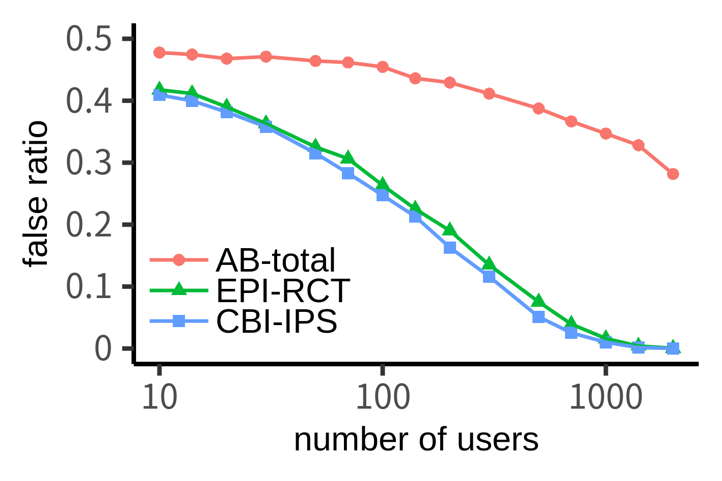
(b) CUBN-T & ULRMF in Dunnhumby.

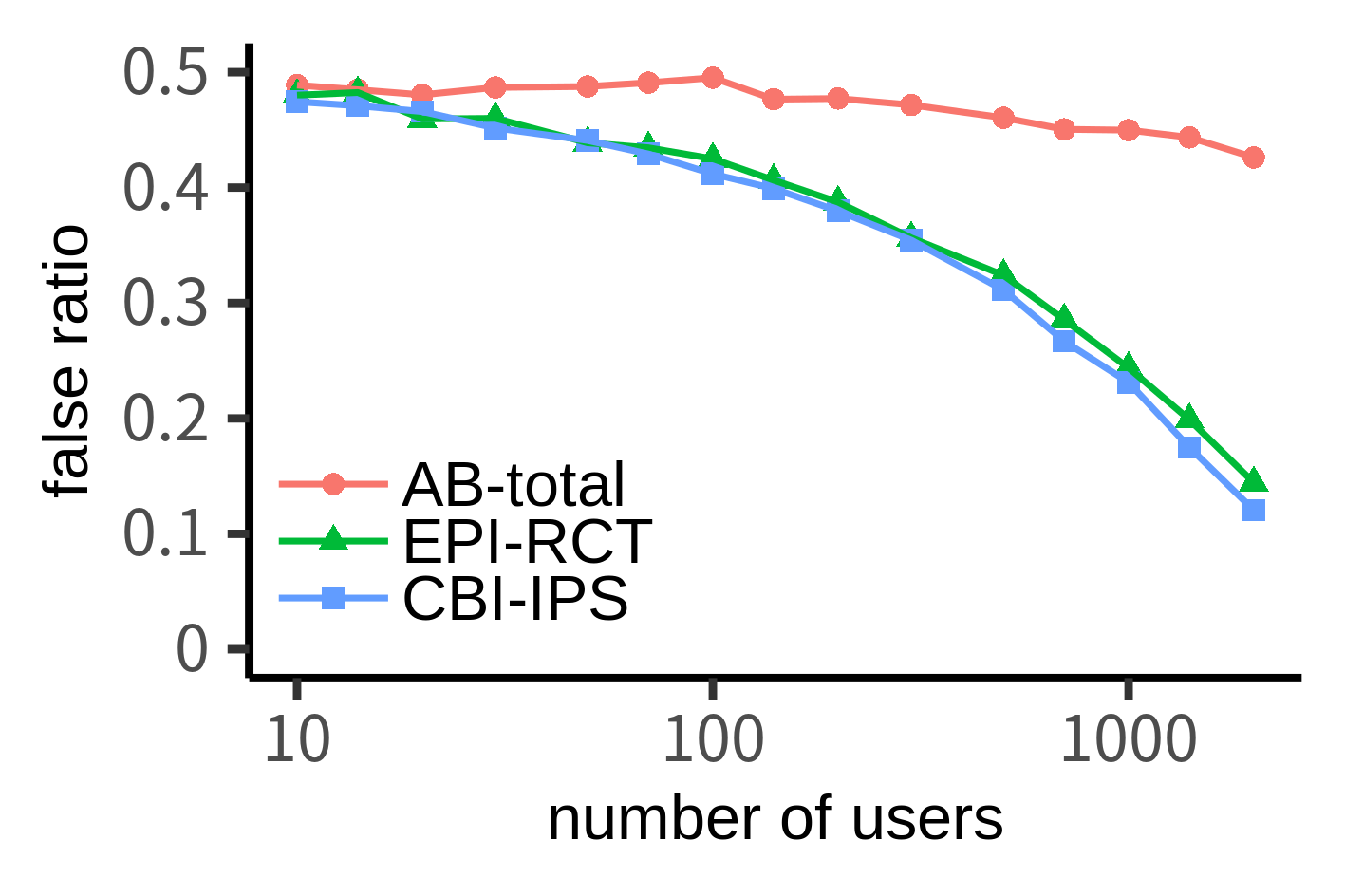
(c) ULRMF & BPR in Dunnhumby.

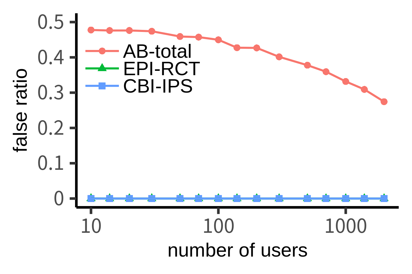
(d) CUBN-O & UBN in ML-1M.

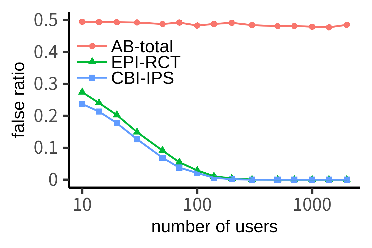
(e) CUBN-O & ULBPR in ML-1M.

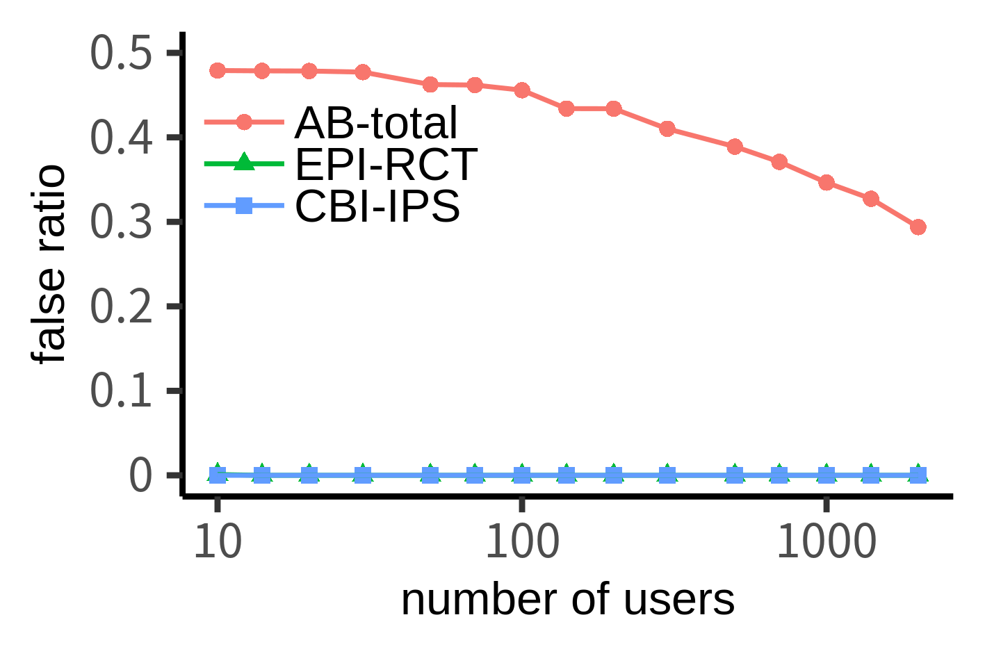
(f) ULBPR & UBN in ML-1M.

Figure 1. Dependence on the number of users.

[The false ratios of the proposed interleaving methods decrease with smaller numbers of users compared to the AB testing method.]In Dunnhumby, the false ratios of AB-total in 2,000 users were about the same with the false ratios of EPI-RCT and CBI-IPS in 70 users. In Movielens-1M, the false ratios of AB-total in 2,000 users were much worse than the false ratios of EPI-RCT and CBI-IPS in 10 users.

5. Conclusions

In this paper, we proposed the first interleaving methods for comparing recommender models in terms of causal effects. To realize unbiased model comparisons, our methods either select items with equal probabilities or weight the outcomes using IPS. We simulated online experiments and verified that our interleaving methods and an A/B testing method are unbiased and that our interleaving methods are largely more efficient than the A/B testing method. In the future, we plan to extend our methods to multileaving. Online experimentation in real recommendation services will also be important for future work.

References

- (1)
- Bodapati (2008) Anand V Bodapati. 2008. Recommendation systems with purchase data. Journal of marketing research 45, 1 (2008), 77–93.
- Bonner and Vasile (2018) Stephen Bonner and Flavian Vasile. 2018. Causal Embeddings for Recommendation. In Proceedings of the 12th ACM Conference on Recommender Systems (Vancouver, British Columbia, Canada) (RecSys ’18). Association for Computing Machinery, New York, NY, USA, 104–112. https://doi.org/10.1145/3240323.3240360
- Chapelle et al. (2012) Olivier Chapelle, Thorsten Joachims, Filip Radlinski, and Yisong Yue. 2012. Large-Scale Validation and Analysis of Interleaved Search Evaluation. ACM Trans. Inf. Syst. 30, 1, Article 6 (March 2012), 41 pages. https://doi.org/10.1145/2094072.2094078
- Chen et al. (2020) Jiawei Chen, Hande Dong, Xiang Wang, Fuli Feng, Meng Wang, and Xiangnan He. 2020. Bias and debias in recommender system: A survey and future directions. arXiv preprint arXiv:2010.03240 (2020).
- Cosley et al. (2003) Dan Cosley, Shyong K. Lam, Istvan Albert, Joseph A. Konstan, and John Riedl. 2003. Is Seeing Believing? How Recommender System Interfaces Affect Users’ Opinions. In Proceedings of the SIGCHI Conference on Human Factors in Computing Systems (Ft. Lauderdale, Florida, USA) (CHI ’03). Association for Computing Machinery, New York, NY, USA, 585–592. https://doi.org/10.1145/642611.642713
- Dias et al. (2008) M. Benjamin Dias, Dominique Locher, Ming Li, Wael El-Deredy, and Paulo J.G. Lisboa. 2008. The Value of Personalised Recommender Systems to E-Business: A Case Study. In Proceedings of the 2008 ACM Conference on Recommender Systems (Lausanne, Switzerland) (RecSys ’08). Association for Computing Machinery, New York, NY, USA, 291–294. https://doi.org/10.1145/1454008.1454054
- Harper and Konstan (2015) F. Maxwell Harper and Joseph A. Konstan. 2015. The MovieLens Datasets: History and Context. ACM Trans. Interact. Intell. Syst. 5, 4, Article 19 (Dec. 2015), 19 pages. https://doi.org/10.1145/2827872
- Hernán and Robins (2020) MA Hernán and JM Robins. 2020. Causal inference: What if. Boca Raton: Chapman & Hill/CRC (2020).
- Hofmann et al. (2011) Katja Hofmann, Shimon Whiteson, and Maarten de Rijke. 2011. A Probabilistic Method for Inferring Preferences from Clicks. In Proceedings of the 20th ACM International Conference on Information and Knowledge Management (Glasgow, Scotland, UK) (CIKM ’11). Association for Computing Machinery, New York, NY, USA, 249–258. https://doi.org/10.1145/2063576.2063618
- Holland (1986) Paul W Holland. 1986. Statistics and causal inference. Journal of the American statistical Association 81, 396 (1986), 945–960.
- Iizuka et al. (2019) Kojiro Iizuka, Takeshi Yoneda, and Yoshifumi Seki. 2019. Greedy Optimized Multileaving for Personalization. In Proceedings of the 13th ACM Conference on Recommender Systems (Copenhagen, Denmark) (RecSys ’19). Association for Computing Machinery, New York, NY, USA, 413–417. https://doi.org/10.1145/3298689.3347008
- Imbens and Rubin (2015) Guido W. Imbens and Donald B. Rubin. 2015. Causal Inference for Statistics, Social, and Biomedical Sciences: An Introduction. Cambridge University Press, New York, NY, USA.
- Jannach and Jugovac (2019) Dietmar Jannach and Michael Jugovac. 2019. Measuring the Business Value of Recommender Systems. ACM Trans. Manage. Inf. Syst. 10, 4, Article 16 (Dec. 2019), 23 pages. https://doi.org/10.1145/3370082
- Joachims (2002) Thorsten Joachims. 2002. Optimizing Search Engines Using Clickthrough Data. In Proceedings of the Eighth ACM SIGKDD International Conference on Knowledge Discovery and Data Mining (Edmonton, Alberta, Canada) (KDD ’02). Association for Computing Machinery, New York, NY, USA, 133–142. https://doi.org/10.1145/775047.775067
- Joachims (2003) Thorsten Joachims. 2003. Evaluating Retrieval Performance Using Clickthrough Data. In Text Mining, Theoretical Aspects and Applications, Jürgen Franke, Gholamreza Nakhaeizadeh, and Ingrid Renz (Eds.). Physica-Verlag, 79–96.
- Lunceford and Davidian (2004) Jared K Lunceford and Marie Davidian. 2004. Stratification and weighting via the propensity score in estimation of causal treatment effects: a comparative study. Statistics in medicine 23, 19 (2004), 2937–2960.
- Ning et al. (2015) Xia Ning, Christian Desrosiers, and George Karypis. 2015. A Comprehensive Survey of Neighborhood-Based Recommendation Methods. Springer US, Boston, MA, 37–76.
- Radlinski and Craswell (2013) Filip Radlinski and Nick Craswell. 2013. Optimized Interleaving for Online Retrieval Evaluation. In Proceedings of the Sixth ACM International Conference on Web Search and Data Mining (Rome, Italy) (WSDM ’13). Association for Computing Machinery, New York, NY, USA, 245–254. https://doi.org/10.1145/2433396.2433429
- Radlinski et al. (2008) Filip Radlinski, Madhu Kurup, and Thorsten Joachims. 2008. How Does Clickthrough Data Reflect Retrieval Quality?. In Proceedings of the 17th ACM Conference on Information and Knowledge Management (Napa Valley, California, USA) (CIKM ’08). Association for Computing Machinery, New York, NY, USA, 43–52. https://doi.org/10.1145/1458082.1458092
- Rendle et al. (2009) Steffen Rendle, Christoph Freudenthaler, Zeno Gantner, and Lars Schmidt-Thieme. 2009. BPR: Bayesian Personalized Ranking from Implicit Feedback. In Proceedings of the Twenty-Fifth Conference on Uncertainty in Artificial Intelligence (Montreal, Quebec, Canada) (UAI ’09). AUAI Press, Arlington, Virginia, USA, 452–461.
- Rosenbaum and Rubin (1983) Paul R Rosenbaum and Donald B Rubin. 1983. The central role of the propensity score in observational studies for causal effects. Biometrika 70, 1 (1983), 41–55.
- Rubin (1974) Donald B Rubin. 1974. Estimating causal effects of treatments in randomized and nonrandomized studies. Journal of educational Psychology 66, 5 (1974), 688.
- Saito et al. (2020) Yuta Saito, Suguru Yaginuma, Yuta Nishino, Hayato Sakata, and Kazuhide Nakata. 2020. Unbiased Recommender Learning from Missing-Not-At-Random Implicit Feedback. In Proceedings of the 13th International Conference on Web Search and Data Mining (Houston, TX, USA) (WSDM ’20). Association for Computing Machinery, New York, NY, USA, 501–509. https://doi.org/10.1145/3336191.3371783
- Sato et al. (2016) Masahiro Sato, Hidetaka Izumo, and Takashi Sonoda. 2016. Modeling Individual Users’ Responsiveness to Maximize Recommendation Impact. In Proceedings of the 2016 Conference on User Modeling Adaptation and Personalization (Halifax, Nova Scotia, Canada) (UMAP ’16). ACM, New York, NY, USA, 259–267. https://doi.org/10.1145/2930238.2930259
- Sato et al. (2019) Masahiro Sato, Janmajay Singh, Sho Takemori, Takashi Sonoda, Qian Zhang, and Tomoko Ohkuma. 2019. Uplift-Based Evaluation and Optimization of Recommenders. In Proceedings of the 13th ACM Conference on Recommender Systems (Copenhagen, Denmark) (RecSys ’19). Association for Computing Machinery, New York, NY, USA, 296–304. https://doi.org/10.1145/3298689.3347018
- Sato et al. (2020a) Masahiro Sato, Janmajay Singh, Sho Takemori, Takashi Sonoda, Qian Zhang, and Tomoko Ohkuma. 2020a. Modeling User Exposure with Recommendation Influence. In Proceedings of the 35th Annual ACM Symposium on Applied Computing (Brno, Czech Republic) (SAC ’20). Association for Computing Machinery, New York, NY, USA, 1461–1464. https://doi.org/10.1145/3341105.3375760
- Sato et al. (2020b) Masahiro Sato, Sho Takemori, Janmajay Singh, and Tomoko Ohkuma. 2020b. Unbiased Learning for the Causal Effect of Recommendation. In Fourteenth ACM Conference on Recommender Systems (Virtual Event, Brazil) (RecSys ’20). Association for Computing Machinery, New York, NY, USA, 378–387. https://doi.org/10.1145/3383313.3412261
- Sato et al. (2021) Masahiro Sato, Sho Takemori, Janmajay Singh, and Qian Zhang. 2021. Causality-Aware Neighborhood Methods for Recommender Systems. (2021), 603–618. https://doi.org/10.1007/978-3-030-72113-8_40
- Schnabel et al. (2016) Tobias Schnabel, Adith Swaminathan, Ashudeep Singh, Navin Chandak, and Thorsten Joachims. 2016. Recommendations as Treatments: Debiasing Learning and Evaluation. In Proceedings of the 33rd International Conference on International Conference on Machine Learning - Volume 48 (New York, NY, USA) (ICML’16). JMLR.org, 1670–1679.
- Schuth et al. (2015) Anne Schuth, Robert-Jan Bruintjes, Fritjof Buüttner, Joost van Doorn, Carla Groenland, Harrie Oosterhuis, Cong-Nguyen Tran, Bas Veeling, Jos van der Velde, Roger Wechsler, David Woudenberg, and Maarten de Rijke. 2015. Probabilistic Multileave for Online Retrieval Evaluation. In Proceedings of the 38th International ACM SIGIR Conference on Research and Development in Information Retrieval (Santiago, Chile) (SIGIR ’15). Association for Computing Machinery, New York, NY, USA, 955–958. https://doi.org/10.1145/2766462.2767838
- Schuth et al. (2014) Anne Schuth, Floor Sietsma, Shimon Whiteson, Damien Lefortier, and Maarten de Rijke. 2014. Multileaved Comparisons for Fast Online Evaluation. In Proceedings of the 23rd ACM International Conference on Information and Knowledge Management (Shanghai, China) (CIKM ’14). Association for Computing Machinery, New York, NY, USA, 71–80. https://doi.org/10.1145/2661829.2661952
- Sharma et al. (2015) Amit Sharma, Jake M. Hofman, and Duncan J. Watts. 2015. Estimating the Causal Impact of Recommendation Systems from Observational Data. In Proceedings of the Sixteenth ACM Conference on Economics and Computation (Portland, Oregon, USA) (EC ’15). ACM, New York, NY, USA, 453–470. https://doi.org/10.1145/2764468.2764488
- Wang et al. (2020) Yixin Wang, Dawen Liang, Laurent Charlin, and David M. Blei. 2020. Causal Inference for Recommender Systems. In Fourteenth ACM Conference on Recommender Systems (Virtual Event, Brazil) (RecSys ’20). Association for Computing Machinery, New York, NY, USA, 426–431. https://doi.org/10.1145/3383313.3412225