Rough McKean-Vlasov dynamics for robust ensemble Kalman filtering
Abstract
Motivated by the challenge of incorporating data into misspecified and multiscale dynamical models, we study a McKean-Vlasov equation that contains the data stream as a common driving rough path. This setting allows us to prove well-posedness as well as continuity with respect to the driver in an appropriate rough-path topology. The latter property is key in our subsequent development of a robust data assimilation methodology: We establish propagation of chaos for the associated interacting particle system, which in turn is suggestive of a numerical scheme that can be viewed as an extension of the ensemble Kalman filter to a rough-path framework. Finally, we discuss a data-driven method based on subsampling to construct suitable rough path lifts and demonstrate the robustness of our scheme in a number of numerical experiments related to parameter estimation problems in multiscale contexts.
1 Introduction
Combining mathematical descriptions of reality with observational data is a key task in economics, science and engineering. In typical applications (such as meteorology [72] or molecular dynamics [85]) there is a hierarchy of models available, ranging from the highly accurate but conceptually and computationally demanding to the approximate but readily interpretable and scalable. Naturally, real-world data is almost always complex, multiscale, and increasingly high-dimensional, whereas the corresponding mathematical abstractions are often preferred to be simple and of comparatively low resolution. The discrepancy between intricate data and reduced-order models poses a significant challenge for their simultaneous treatment, and the failure of some standard statistical approaches in scenarios of this type is well documented [2, 97, 104, 119, 121].
Robustness to model misspecification and perturbation of the data is a central concept in the design of statistical methodology capable of bridging scales: Consider a statistical model – to be thought off as simple – generating (time-dependent) data and a corresponding algorithmic procedure producing the output . We expect that deals adequately with complex data in the case when it is continuous in an appropriate sense. Indeed, might be a simplified description of an underlying model family , where the formal limit encapsulates the passage from a complex to a reduced description. The output on ‘real-world’ data is then close to by continuity even though has been contructed on the basis of .
Unfortunately, in various contexts (for instance, in parameter estimation for diffusions [43] and stochastic filtering [10]) the map is given in terms of stochastic integrals against which are well known to be discontinuous with respect to standard topologies [57, 59]. The theory of rough paths provides a principled route towards constructing continuous modifications of (employed, for instance, in [30, 43]) by replacing stochastic integrals in terms of rough integrals defined on appropriately lifted paths . Although the difficulty of obtaining or imposing the additional information is well known (see, however, [9, 52, 86] and Section 6 of this article), recent works have demonstrated the potential of including path signatures into data-driven methods to compress information efficiently or unveil multiscale structure [21, 91]. Moreover, the rough path perspective provides refined insights into misspecification of diffusion models: Indeed, two paths may be ‘similar in a classical sense’ (for instance, in supremum norm) in spite of their associated lifts exhibiting a large rough path distance, in turn leading to inaccurate inferences. In Section 6 we discuss how those discrepancies can be compensated in a systematic and data-driven manner.
In this paper, we follow the rough path paradigm just described and develop a robust version of the Ensemble Kalman Filter (EnKF) [16, 51], drawing on a reformulation of the Kushner-Stratonovich SPDE for stochastic filtering [10] in terms of McKean-Vlasov dynamics (known as the feedback particle filter [99, 112, 116]). The EnKF is a versatile approximate procedure for Bayesian inference that is observed to perform particularly well in high-dimensional settings [108] and has recently been applied to problems in machine learning [63, 105]. Our analysis includes the case when the model and observation noises are correlated as this is precisely the setting in which significant obstacles in the construction of robust filters are known to occur [30]. Furthermore, as shown in [95] and recalled in Appendix B, stochastic filtering with correlated noises is a natural generalisation of maximum likelihood parameter estimation for diffusions in the context of inexact measurements. In this setting, we discuss the relationship between subsampling-based approaches to multiscale parameter estimation [104] to the task of estimating the Lévy area in a rough paths approach.
The construction put forward in this paper requires the formulation of McKean-Vlasov equations in a rough path setting (as studied first in [19] and more recently in the twin papers [7, 8], both considering the dynamics to be driven by a random rough path). The approach introduced in [27] is more suitable for our needs as it allows a clear separation between independent Brownian motions and a common deterministic noise. However, the assumptions in [27] do not cover unbounded coefficients, while the common noise coefficient may depend on both the state of the solution and its law. In equation (11) considered below, the coefficient only depends on the law of , which simplifies the problem to some extent, but also allows us to use a different approach, where we treat the stochastic and the rough integrals in two separated steps. As it will become clear from the proofs in Section 4.4, there is no need to create a joint rough path (or rough driver). All previous works on rough McKean-Vlasov equations deal with bounded globally Lipschitz-continuous (actually smoother) coefficients. These results cannot be applied here, as the coefficient has linear growth in the measure of the solution and is locally-Lipschitz with Lipschitz constant depending on the moments of the solution.
1.1 Setting and main results
In this section we specify the exact setting and present our main results. Throughout the paper we fix a filtered probability space satisfying the usual conditions and consider the following filtering model,
| (1a) | |||||
| (1b) | |||||
In the above display, (1a) represents the (hidden) signal, whereas (1b) specifies the available observations. Note straight away that the signal noise and the observation noise may be correlated. We assume that the signal is -dimensional, that is, , and that the observations are -dimensional, . In applications it is often the case that . The maps and are assumed to be sufficiently regular (see below). We assume , to be symmetric nonnegative definite and . Furthermore, and denote independent - and - dimensional standard Brownian motions, respectively. Lastly, we assume that the observation covariance
| (2) |
is strictly positive definite. Defining the observation -algebras
| (3) |
where is the collection of -null sets, our objective is to compute or approximate the filtering measures
| (4) |
for bounded and measurable test functions ; we refer to [10] for technical details.
As a step towards tractable numerical approximations of (4), we follow [95] and introduce the McKean-Vlasov equation
| (5) |
where (resp. ) is a given -dimensional (resp. -dimensional) Brownian motion, both independent from and . Denoting by the conditional law with respect to the common noise of solutions to (5), the coefficients and are required to solve the following partial differential equations,
| (6) |
and
| (7) |
for and -almost surely, where . Moreover, the common noise coincides with the observation process (1b) and the integral in is understood in the sense of Stratonovich.
The construction of the system (5)-(7) as well as existence of solutions will be detailed in Section 2.4. The filtering problem and the McKean-Vlasov equation (5) are related in the following way.
Proposition (formal, see Proposition 2.1).
If admits a density and the solution to (5) is unique, then , -a.s. for every .
Reformulations of the filtering problem in terms of McKean-Vlasov dynamics similar to (5)-(7) have been introduced in [32, 116], further analysed in [99], and are commonly referred to as feedback particle filters; the formulation (5)-(7) combines Stratonovich integration (as in [99]) with a stochastic innovation term (as in [106, Section 4.2]) so as to allow for a transition to geometric rough paths in the setting of correlated noises (as in [95]).
One of the practical challenges posed by the system of equations (5)-(7) is solving the PDEs (6) and (7) in and for a given measure . As has been shown in [112] for a similar system of equations, replacing and by their best constant-in-space approximations in least-square sense recovers a version of the Ensemble Kalman filter dynamics [16]. We follow this approach (see Lemma 2.2 below) and replace the coefficient by , explicitly defined as
| (8) |
where refers to the set of probability measures on . Similarly, we replace by , defined as
| (9) |
which can be interpreted as an Itô-Stratonovich correction term.111Indeed, the system (10) can be recognised as the Stratonovich version of the EnKF, see Appendix C. Thus, we obtain the system
| (10) |
where . This equation is well posed according to Lemma 4.18 below.222In this paper, we assume to be bounded, circumventing difficulties with the non-Lipschitzness of in the case when is unbounded. For results addressing this challenge (although in slightly different settings), we refer the reader to [38, 39, 41, 46, 71, 80, 81, 82, 83].
In order to construct a robust filter, we replace the common noise in equation (5) by a deterministic rough path with regularity . As explained in the introduction, the rationale is that the solutions to rough differential equations are expected to be continuous in the rough path driver (see [57]), in contrast to the Itô solution map associated to stochastic differential equations. Moreover,
using a deterministic path is natural since we are conditioning on the observation, that we can assume to be given and deterministic.
Applying the modifications from the preceding two paragraphs to equation (5) we obtain the system
| (11) |
From Lemma 4.13 below, the path is controlled by with Gubinelli derivative [57, Definition 4.6]
| (12) |
so that the rough integral in equation (11) will make sense (see Section 3.3 below for an overview on controlled rough paths). Moreover, when is a semimartingale with covariance , for , the correction between the Stratonovich and Itô rough path lift is given by , which corresponds to , see Appendix C.
Our main result is the following well-posedness and stability theorem for (11).
Theorem 1.1.
The proof is a consequence of the results in Section 4.4 and can be found at the end of that section. Associated to the McKean-Vlasov equation (11) we also study the following system of mean-field interacting particles,
| (13a) | ||||
| (13b) | ||||
where is the empirical measure of the system and is the canonical lift of a differentiable and bounded path with bounded cadlag derivative. We have the following well-posedness and convergence result for the interacting particles.
For results concerning similar mean-field limits in the classical setting we refer to [46, 45, 82]. The preceding two theorems suggest that numerical methods based on the interacting particle system (13) are robust to perturbations in the data, and hence suitable for applications in multiscale contexts as described in the introduction. Inspired by Davie’s work [33], we propose the following recursive numerical scheme,
| (14a) | ||||
| (14b) | ||||
in the following referred to as the Rough-Path Ensemble Kalman Filter (RP-EnKF). Here, is the step size, and and denote independent zero mean Gaussian random variables of dimensions and , respectively. The precise form of the estimator versions , and will be detailed in Section 6. Finally, the first term in (14b) is built after the Gubinelli derivative from (12), with its precise meaning given by
| (15) |
Crucially, the scheme (14) takes the lifted component (representing iterated integrals of the path ) as an input. This dependence allows our methodology to appropriately take into account multiscale structure and other information encoded in the signature (such as discrepancies due to model misspecification), but also necessitates appropriate ways to estimate from data. We will discuss this in more depth in Sections 2.3 and 6, but note here that it is natural to decompose into its symmetric and skew-symmetric part
| (16) |
The form of the symmetric part is suggested by the requirement that the lifted path is geometric,
| (17) |
in particular this expression can readily be computed from discrete-time observations . The difficulty thus resides in estimating the Lévy area contributions (or corrections) . We suggest a subsampling-based method, establishing connections to multiscale parameter estimation as investigated in [104]; see Section 2.3. Other approaches towards obtaining have been developed in [9, 52, 86]. We would like to stress that although estimating works reasonably well in our experiments (see Sections 6.1 and 6.2), in many applications it might yield satisfactory results to neglect the skew-symmetric part, that is, to use the approximation , either because the observation path is one-dimensional, or because the Lévy area term is comparatively small (see Section 6.3). In these cases, the RP-EnKF can be implemented straightforwardly without additional estimation steps, and represents a robust Stratonovich-version of the EnKF (see Appendix C).
Itô, Stratonovich and rough integrals. Before concluding this introduction, let us comment on the difference between the RP-EnKF scheme (14) and the more conventional EnKF updates
| (18) |
see [16, 51, 108]. Clearly, (14) and (18) coincide up to the terms in (14b). This difference can be attributed to alternative (but equivalent) perspectives on the underlying continuous-time dynamics, and hence we expect the terms in (14b) to cancel each other in the limit as , when is obtained at discrete time-points from (1b) and are the increments of the Stratonovich lift corresponding to piecewise linear approximation (that can be computed according to (17) and setting ). Indeed, (18) corresponds to the Euler-Maruyama discretisation of the McKean-Vlasov SDE
| (19) |
understood in the sense of Itô. In contrast, the term in (14b) can be seen as an Itô-Stratonovich correction to (19), see Appendix C, while the first term in (14b) arises from a Milstein-type approximation scheme for Stratonovich SDEs [73, Section 10.3] (or as part of the discrete approximation of rough integrals according to Davie [33]). The equivalence of the classical and the rough path version, that is, of (10) and (11), is stated in Lemma 4.18.
The distinction between (14) and (18) becomes important when the data and is described by (1) only in an approximate sense and hence robustness becomes a key issue.
Importantly, the passage to rough integrals is indispensable for the continuity statements in Theorem 1.1 and the numerical robustness of the RP-EnKF scheme demonstrated in Section 6. The Stratonovich picture is natural in view of the Wong-Zakai theorem [58, Section 9.2] and determines the symmetric part in (16) as can then be interpreted as a geometric rough path (see (17) and Section 6). Our approach of replacing Itô by Stratonovich and subsequently rough integrals mirrors the construction in [43] in the context of maximum likelihood parameter estimation for diffusions.
Our contributions and structure of the paper. Our main contributions are as follows:
-
•
Based on the prior works [95, 99, 106], we derive the McKean-Vlasov system (5)-(7), incorporating a stochastic innovation term as well as correlated model and observation noise. Crucially, the dynamics (5)-(7) is given entirely in terms of Stratonovich integrals that allow the construction of robust filtering schemes built on geometric rough paths.
- •
-
•
We show well-posedness as well as propagation of chaos of the interacting particle approximation (13).
-
•
We suggest the RP-EnKF scheme (14) and in particular devise a subsampling based method to estimate the lift components from data (as corrections in a model misspecification scenario). The robustness of the RP-EnKF (and the nonrobustness of the EnKF) is demonstrated using numerical examples in the context of combined state-parameter estimation.
In Section 2 we review the most relevant results in filtering theory, we motivate the use of the McKean-Vlasov equation and explain the concept of a robust filter. In Section 3 we introduce common notation and recall some background on rough paths. In Section 4.4 we present the analysis of the rough McKean-Vlasov equation (11), which includes well-posedness and stability. In Section 5 we treat the interacting particles system (13) and prove well-posedness and propagation of chaos. In Section 6 we detail the construction of the numerical scheme, including a presentation of our subsampling approaching towards estimating the Lévy area. Finally, we conclude the paper with some numerical experiments.
2 Background in filtering, robust representations and McKean-Vlasov dynamics
In this section we discuss essential background on robust filtering and put our work into perspective. Section 2.1 will summarise existing approaches towards solving the filtering problem posed by (4), both from a theoretical as well as from an algorithmic perspective. In Section 2.2 we review the challenges to these methods posed by perturbations in the observed data , leading to the concept of robustness. In Section 2.3 we draw connections of the McKean-Vlasov approach considered in this paper to maximum likelihood based techniques for stochastic differential equations, in particular to the methods developed in [43]. Finally in Section 2.4 we make our McKean-Vlasov formulation as well as the ensemble Kalman approximation precise.
2.1 Solutions to the filtering problem and algorithms
It is well known that the measure defined in (4) is a measurable function of the observation path and can be obtained as a solution to the Kushner-Stratonovich SPDE [10, Section 3.6],
| (20) |
where
| (21) |
denotes the infinitesimal generator associated to the signal process (1a).
From the computational viewpoint, numerically solving (20) directly (for instance, using grid-based methods) is usually infeasible, especially when the dimension is large (see [10, Section 8.5] for a discussion). Many algorithmic approaches therefore rely on the simulation of carefully constructed interacting particle systems, positing the corresponding (possibly weighted) empirical measures as approximations for .
Sequential Monte Carlo methods rely on Bayes’ theorem in order to approximate the conditional expectations (4). More precisely, defining the likelihood
| (22) |
the filtering measures admit the representation
| (23) |
according to the Kallianpur-Striebel formula [10, Proposition 3.16]. Consequently, approximations of can be obtained by sampling from the signal dynamics (1a) in conjunction with appropriate weighting and/or resampling steps on the basis of (22). For detailed accounts, we refer the reader to [48, 40, 108]. While sequential Monte Carlo methods reproduce the filtering measures exactly in the large-particle limit (see, for instance, [10, Theorem 9.15]), they tend to become unstable in high-dimensional settings due to weight collapse: the conditional and unconditional laws of are often so distinct as to render reweighting-based approaches infeasible due to low effective samples sizes.
Ensemble Kalman filters (EnKFs) [108, Section 7.1] can be formulated in terms of interacting or mean-field (McKean-Vlasov) diffusions. In the case when (that is, when the signal and observation noises are uncorrelated [109, Section 7.1], [15]) the basic EnKF due to Evensen [17, 50, 51] is given by
| (24) |
with
| (25) |
or a standard particle approximation thereof. The system (24)-(25) is motivated by the fact that the corresponding law reproduces exactly in the linear Gaussian case: If is Gaussian, and for appropriate matrices and , then remains Gaussian for all , and . In cases where the preceding conditions are not satisfied, the system (24)-(25) becomes an approximation, the accuracy of which is far from well understood theoretically. However, the ensemble Kalman approach has empirically proven to be both fairly reliable in nonlinear settings as well as scalable to high-dimensional scenarios, and therefore nowadays constitutes one of the workhorses in practical data assimilation tasks [108]. We refer to [16] for a recent review of its theoretical properties.
The more recently proposed feedback particle filters [32, 112, 116] rely on carefully designed McKean-Vlasov diffusions of the type (24) such that the associated (conditional, nonlinear) Fokker-Planck equation coincides with the Kushner-Stratonovich SPDE (20). By construction, such models are exact, and the conditional laws induced by the solutions to feedback particle filter dynamics provide the filtering measures (4). As an illustration,
| (26) |
was suggested in [106] and extended in [95], where is determined from the elliptic PDE
| (27) |
and is an appropriate correction term (see Section 2.4 for an in-depth discussion). Clearly, the systems (24)-(25) and (26)-(27) are strongly related in spirit, combining a replication of the signal dynamics (1a) with a data-dependent nudging term so as to match the observations. Reiterating the discussion so far, solutions to (26)-(27) provide exact solutions to the filtering problem (4), while solutions to (24)-(25) lead to approximate ones (except in the linear Gaussian case). However, as is given explicitly in (25), the system (24)-(25) lends itself straightforwardly to efficient numerical integration, while the system (26)-(27) poses a formidable numerical challenge in the form of the high-dimensional PDE (27). What is more, well-posedness of systems of the type (26)-(27), with coefficients that depend on the law through the solution of a PDE is currently not well understood. Nevertheless, McKean-Vlasov formulations of the type (26)-(27) conveniently link between the theoretically optimal Kushner-Stratonovich SPDE (20) and the numerically tractable and practically relevant ensemble Kalman dynamics (24)-(25). In this paper, we leverage this viewpoint in order to construct a robust version of (18).
2.2 Robust filtering
In order to model and solve real-life problems it is highly desirable that the conditional law (or any numerical approximation thereof) depends continuously on the observation path : This property would ensure robustness against misspecification of the underlying signal and observation dynamics (as is typical in reduced-order modeling) as well as against anomalies or artefacts in the collection of the data (such as discretisation errors or perturbation by noise), see [10, Chapter 5] for an overview,
[22, 23, 34, 78, 36, 37, 35]
and Section 2.3 below.
Unfortunately, however, the -dependent measurable map provided by (4) can be shown to be neither unique nor continuous [30] in standard topologies. At a fundamental level, this problem is due to the appearance of stochastic integrals against in (20) and (22) which are well known to induce classically discontinuous maps (for instance, in the supremum norm), see [57, 59]. In order to address this issue and to obtain a continuous333As pointed out in [30], the continuity requirement restores the uniqueness of the map . version of the process , Clarke suggested using (stochastic) integration by parts in (22) in order to eliminate the -dependence [22]. Notably, this approach is restricted to the case when the signal and observation noises are independent (that is, ), see [22, 23, 78], or the case when the observation is one-dimensional (that is, ), see [34, 36, 37, 35, 53]. Addressing the situation of multidimensional correlated observations, the authors of [30] showed by means of a counter-example (see [30, Example 1]) that continuity as a function of is impossible to achieve. Instead, they
use rough path lifts and establish continuity when is considered as a function of the augmented observation path. Similar ideas have been pursued in [64, Theorem 5.3], putting forward the notion of ‘good’ approximations of the observation path. As the aforementioned works are concerned with the likelihood (22), these lay the foundations for the development of robust sequential Monte Carlo methods as reviewed in Section 2.1, and the recent preprint [31]
explores that direction.
We would also like to mention the works [44, 66] that allow treating the Zakai SPDE (governing the unnormalised filtering distribution [10, Section 3.5]) in a rough paths framework, however noticing that the numerical treatment of SPDEs is faced with enormous challenges, in particular in high-dimensional settings. Some other works addressing issues in robust or multiscale filtering include [3, 4] (assuming uncertainty in the coefficients) as well as a sequence of works by N. Perkowski and coworkers in the context of averaging and homogenisation [14, 12, 13, 68, 69, 88, 87, 117, 118].
In this paper, we instead construct a robust version of the ensemble Kalman filter (24)-(25) on the basis of its connections to feedback particle formulations as in (26)-(27). Before describing our strategy, we review related work on maximum likelihood parameter estimation for stochastic differential equations.
2.3 Parameter estimation and filtering in multiscale systems
In this section we present a prototypical example that illustrates some of the challenges in robust filtering as well as the scope of the methods developed in this paper, following [95]. Consider the SDE
| (28) |
where , and is a parameterised drift vector field, with parameter set . The objective is to find the true parameter from a noisy realisation of , that is, we assume that the observation process is given by
| (29) |
As before, denotes the observation noise covariance, and stands for a standard -dimensional Brownian motion. The problem setting (28)-(29) can be brought into the form (1) by elevating to a time-dependent variable, that is, by setting , hence viewing (28)-(29) as a combined state-parameter estimation problem, see [95]. Accordingly, and are then given as and , and the matrices and take the form
| (30) |
Finally, the filtering formulation is completed by specifying a prior distribution on the initial condition . The resulting filtering measures encode the Bayesian posterior on the combined variable . Consequently, the -marginals provide meam a posteriori estimates on the parameter of interest as well as corresponding bounds on Bayesian uncertainty.
In the particular case when the path is observed without contamination by noise, that is, , and is linear444For simplicity of the presentation, we also assume here that is one-dimensional, that is, . in , that is, with satisfying appropriate nondegeneracy conditions [43], the parameter can be recovered from the maximum likelihood estimator
| (31) |
in the limit when , see [79, 89]. Furthermore, in this case the McKean-Vlasov dynamics suggested in this paper can be solved explicitly, and the corresponding means are directly related to (31), see Appendix B and [95]. It is well known that the estimator (31) can be inaccurate when evaluated on paths that only approximately satisfy (28), for instance when (28) represents a reduced description of an underlying multiscale dynamics [2, 104, 121]. A common approach towards addressing this problem is to subsample the data, see [1, 5, 6, 60, 61, 70, 74, 75, 98, 103] for methodological aspects. For specific applications see [93] (multiscale inverse problems), [2, 97, 121] (economics and finance), and [28, 119] (ocean and atmospheric science).
A different approach towards robustness of the estimator (31) has been taken in [43], addressing the discontinuity of the Itô integral . To resolve this issue, the authors suggest replacing Itô by Stratonovich integration (motivated by the Wong-Zakai theorem [57, Theorem 9.3] and entailing a correction term involving ), and subsequently using rough paths integration instead of Stratonovich integration (relying on a suitable lift ). The resulting estimator
| (32) |
can then be shown to be continuous as a map from to . The construction of the RP-EnKF dynamics (14) follows a similar line of reasoning, but our approach is applicable to situations where the path is contaminated by noise () and where is nonlinear in . The latter generalisation makes our method suitable to applications involving deep learning, that is, when the drift in (28) is parameterised by a neural network as in [63]. We discuss the idea of subsampling the observed data path in the context of constructing an appropriate rough path lift in Remark 6.2 below in Section 6.
2.4 From the filtering problem to the McKean-Vlasov equation
In this section, we discuss the construction of the McKean-Vlasov system (5)-(7) and the nature of the approximation in (10) and (11). The general idea goes back to [32, 116], and various modifications have been proposed in [95, 99, 106]. Our formulation combines Stratonovich integration (as in [99]) in order to later invoke Wong-Zakai type approximation results with a stochastic innovation term (as in [95, 108]) as required for the case of correlated model and observation noise. For the sake of clarity, we repeat the PDEs (6) and (7) in their respective index forms (using Einstein’s summation convention),
| (33) |
and
| (34) |
In the case when model and observation noise are uncorrelated (), testing (33) with reveals that the system (33)-(34) is equivalent to the system (2.5)-(2.6) obtained in [99]. The McKean-Vlasov system (5)-(7) solves the filtering problem in the following sense:
Proposition 2.1.
Let , assume that the system (1) admits a unique solution and that the Zakai equation associated to the corresponding filtering problem is well posed. Let be the conditional law of given as defined in (4) and assume that admits a -density with respect to the Lebesgue measure, -a.s., for all Moreover, assume that the McKean-Vlasov equation (5) admits a unique solution such that its conditional law admits a -density with respect to the Lebesgue measure, -a.s.. Assume that and are predictable stochastic processes with values in and , respectively, independent from and , and such that the PDEs (6) and (7) are satisfied, -a.s.. Then , for all .
To prove Proposition 2.1, we define the unnormalised conditional law associated to the McKean-Vlasov dynamics (5),
| (35) |
where the likelihood is defined in (22). Comparing the evolution of with the solution of the Zakai equation [10, Section 3.5] allows us to derive the PDEs (6) and (7). This approach allows us to circumvent the stringent regularity condition in [99, Assumption 3.4]. For details see Appendix A.
One of the numerical challenges posed by the system of equations (5)-(7) is to obtain (approximate) solutions and to the PDEs (6) and (7). We sidestep this problem by using constant-in-space approximations leading to the system (10) of ensemble Kalman filter type. A similar correspondence has been observed in [112] and is optimal in the following sense:
Lemma 2.2.
Let and be a (weak) solution to (6). Denote by the best constant approximation in least-squares sense, that is
| (36) |
where denotes the Frobenius norm. Then is given by
| (37) |
Moreover, let be a solution to (7) with replaced by . Then the best constant approximation of in least-squares sense (with respect to the Euclidean norm) is given by
2.5 Literature on McKean-Vlasov dynamics
McKean-Vlasov equations are stochastic differential equations whose coefficients depend on the law of the solution. They are sometimes called law-dependent equations. McKean-Vlasov equations have been the subject of several studies starting from the seminal work of McKean [92] and Dobrushin [47]. McKean-Vlasov equations arise as limit of mean-field interacting particle systems, when the number of particles goes to infinity. For a general introduction on the topic we refer the reader to Sznitman [111].
In recent years there has been an increased interest in mean-field particles with common noise, see [25, 76, 77] or [18] in the case of mean-field games. In these type of systems the particles are subject to the same random perturbation and possibly additional independent noises. There is no averaging effect of the common perturbation when the number of particles increases. The limit object is again a law-dependent SDE, but this time the coefficient depends on the conditional law of the solution given the common noise. This is the case for equation (11), where the coefficients and depend on the law of given .
McKean-Vlasov equations from a rough path perspective were studied for the first time in [19] and more recently in the twin papers [7, 8]. In both of these works the equation is driven by a random rough path that is quite general and can describe the independent noise, the common noise or both. This gives the additional difficulty of needing to keep track of the rough path as a -valued path. In [19] only the drift of the equation depends on the law of the solution, the coefficients in front of the noise depend only on the state of the solution. The more recent work [8] generalises that approach to include law-dependent coefficients. The authors use the approach by Gubinelli on controlled rough paths (see Section 3.2 for a brief introduction on the topic). In order to do this, they need Lions’ approach to calculus in measure spaces endowed with the Wasserstein metric. The equation is then solved as a fixed-point in the mixed and -space. In [24] the case of pathwise McKean-Vlasov equation with additive noise is considered. The basic techniques used are similar to the ones used in the rough-path case, but the need for rough paths is removed thanks to the additive noise. See also [114].
McKean-Vlasov equations with a rough common noise have been studied recently in [27]. This is the first time that a rough McKean-Vlasov equation is studied when there is a clear separation between independent Brownian motions and a common deterministic noise. In [27], the common noise coefficient depends on both the state of the solution and its law. In equation (11), the coefficient only depends on the law of , which simplifies the problem to some extent, but also allows us to use a different approach, where we treat the stochastic and the rough integrals in two separated steps. As it will be clear from the proofs in Section 4.4, there is no need to create a joint rough path (or rough driver). All previous works on rough McKean-Vlasov equations deal with bounded coefficients, which cannot be applied here, as the ceofficient has linear growth in the measure of the solution.
Very recently the authors of [58] developed a theory of mixed rough and stochastic differential equations under Lipschitz and boundedness conditions on the coefficients and they plan to address the application to McKean-Vlasov equations with common noise in a forthcoming paper.
3 Preliminaries
3.1 Notation
Given a metric space , we call the space of probability measures on . For we denote by the mean of and by the integral of a measurable function in .
Let , if is a normed space with norm and , we denote by
the -moment of and the -central moment of , respectively. For , we call the space of probability measures on such that . We endow this space with the -Wasserstein metric
where is the set couplings between and . For ease of notation, we denote by the Wasserstein metric on and by the Wasserstein metric on . Given a function and a path , we define
where . If , we use the following notation for the Taylor expansion
Throughout the paper we use for the usual Fréchet derivative and . We sometimes use the notation . For a stochastic process on a filtered probability space , we denote the conditional expectation by .
3.2 Background in rough paths
The theory of rough paths is a framework that allows well-posedness and stability properties for equations of the form
| (38) |
where is a path of regularity lower than the regularity assumptions amenable to classical calculus. For , we denote by the set of all continuous functions
such that there exists a constant with and we denote by the infimum over all such constants. We denote by the -Hölder norm. We write for the set of paths such that , where we have defined .
A rough path is a pair such that
| (39) |
We equip with its subset topology which we shall call the rough path topology. Relation (39), commonly referred to as Chen’s relation, encodes the algebraic property between a path and its iterated integral, viz the formal equality
When the above integral is in general not canonically defined using functional analysis. However, in the case of being a sample path of the Brownian motion, , one can use probability theory to define iterated integrals using e.g. Itô integration or Stratonovich integration. We denote by and these (random) rough paths, respectively. It is classical that
| (40) |
The Stratonovich rough path is an example of a geometric rough path, that is to say it is in the closure in the rough path topology of the image of the mapping
defined on .
Given two rough paths we define the following distance,
We refer the reader to [57] for a more comprehensive discussion of the rough paths notations and concepts used in this paper.
3.3 Controlled rough paths and rough differential equations
To use rough paths for a solution theory of equations of the form (38), which we rewrite with the formal expression
| (41) |
we start with the ansatz that the solution takes the form of a Taylor-like expansion
| (42) |
where is of higher regularity than , and is the so-called Gubinelli derivative. We denote by the set of all pairs such that implicitly defined via (42) satisfies , which also induces the topology on .
The sewing lemma provides a continuous integration mapping
where
satisfies for some constant only depending on . A solution of (41) can now be defined as a fixed point of the composition of the mappings
From the sewing lemma and the definition of the integration mapping we see that we could equivalently define the solution of (41) as a path such that
satisfies . The latter formulation is usually referred to as Davie’s expansion/solution.
4 Stochastic rough McKean-Vlasov equations
In this section, unless otherwise specified we fix and . Moreover, is a complete filtered probability space that supports a standard -dimensional Brownian motion . Recall that for , we call the -moment of and the -central moment of .
4.1 McKean-Vlasov SDEs with linear growth in the measure
Consider the measurable functions and satisfying the following assumptions:
Assumption 1.
Assume that there exists a constant such that
-
(i)
(linear growth) , ,,
(43) -
(ii)
(locally Lipschitz) , , ,
(44)
Consider the following McKean-Vlasov equation,
| (45) |
where is an -dimensional Brownian motion.
Lemma 4.2.
Proof.
To prove well-posedness we use a Picard-type argument. For and , we define
Let . We define the following stochastic differential equation
| (46) |
By our choice of and Assumption 1, the coefficients and are bounded and Lipschitz. By standard theory this equation admits a unique strong solution on the interval , which we denote by . This solution has continuous sample paths, -a.s.. We are ready to define the map
Using standard stochastic calculus estimates, Assumption 1 and Gronwall’s lemma we obtain the following upper bound on the second moment,
| (47) |
where is a generic constant that only depends on the coefficients and . Let us now take , with this choice we have . This implies . Using again stochastic calculus and Gronwall’s lemma, we have that for each ,
| (48) |
Here is again a generic constant depending only on and , possibly different than before. Also notice that are measures on the path space and in the left-hand side of (48) we are considering, with an abuse of notations, their projections on .
Iterating times the inequality (48), we obtain
For the choice of , if we take large enough, we have that the map is a contraction on . By the Banach fixed point theorem, has a unique fixed point on , which is the unique solution to equation (45) up to time .
Global existence and uniqueness follow by iterating this argument on intervals of fixed length , which does not depend on the value of the initial condition, but only on the assumptions on the coefficients of the equation. ∎
4.2 The common noise case
Consider measurable functions and as in the previous section and , each of which satisfying the following assumption on their respective domain.
Assumption 2.
Let be a Banach space, for assume that there exists a constant such that
-
(i)
(linear growth) ,
(49) -
(ii)
(locally Lipschitz) , ,
(50)
Notice that, since is independent of the space variable , condition 2 (ii) reduces to local Lipschitz continuity in the measure variable.
Consider the following McKean-Vlasov equation,
| (51) |
where is the -dimensional Brownian motion fixed at the beginning of the section and is an -dimensional Brownian motion adapted to . Assume that are independent. In (51), is the conditional law of the solution given the filtration generated by the common noise .
Lemma 4.3.
Proof.
It follows from the independence of , and that
Let , we have
Set , as an application of Itô’s formula we have
By using Assumption 2 (i) also on the drift, we obtain
Gronwall’s lemma gives , where is a constant depending on . A similar bound can be obtained for .
Combining the upper bounds on the central moment with Assumption 2, we have global Lipschitz continuity and boundedness of the coefficients . With standard estimates and Growall’s lemma one can show that , which implies intistinguishability of the processes and . ∎
4.3 McKean-Vlasov with continuous deterministic forcing
Let and be measurable functions satisfying the following assumptions:
Assumption 3.
Assume that there exists a constant such that
-
(i)
(linear growth) ,
(52) -
(ii)
(Lipschitz continuity) , ,
(53)
Let be a continuous bounded function, and consider the following stochastic differential equation,
| (54) |
Definition 4.5.
A stochastic process on is a solution for equation (54) with initial condition if is predictable and for every , the following integral equation is satisfied -a.s.,
Remark 4.6.
In the following, we will construct an adapted solution with continuous sample paths. Since is Lipschitz continuous, we immediately have that is predictable and the Itô integral is well defined.
Let be a solution to equation (54), we define . We start with some preliminary expansions and estimates for . We have, for ,
| (55) |
Lemma 4.7.
Let and . There exists a constant such that as and
Moreover, for and , we have
Proof.
Using standard estimates and the Burkholder-Davis-Gundy (BDG) inequality on equation (55) we have
The first inequality follows from a standard application of Gronwall’s lemma. For the second inequality we use again BDG and Jensen’s inequality to obtain
The second inequality as well as the condition on follows from the Kolmogorov continuity theorem [57, Theorem 3.1]. ∎
Remark 4.8.
The bounds in Lemma 4.7 do not depend on the forcing term . This gives us a good a-priori bound on the solution. Let be fixed and arbitrarily large and assume that there exists such that . Then there exists a global constant such that
| (56) |
We have the following a priori estimates.
Lemma 4.9.
Let . Given and , we call a solution to equation (54) with forcing and initial condition .
Let satisfy Assumption 3. Then there exists a constant such that as and
| (57) |
Given and , there exists a positive constant such that
| (58) |
Proof.
We write and omit here the dependence of the process on and as there is no possibility of confusion in the first part of the proof. Using Jensen’s inequality, the Burkholder-Davis-Gundy inequality and Assumptions 3 we have the following estimate for ,
where the constant depends only on and . Equation (57) follows immediately using the bounds in Lemma 4.7.
In addition the the previous bounds, if the forcing term is -Hölder continuous, we have that also the solution is -Hölder continuous.
Lemma 4.10.
Let and . Assume that and . Then there exist such that as and
| (59) |
Moreover,
| (60) |
Proof.
We write and omit here the dependence of the process on as there is no possibility of confusion in the first part of the proof. Using Jensen’s inequality, the Burkholder-Davis-Gundy inequality and Assumption 3 we have the following estimate for ,
The constant is such that , as . We apply Lemma 4.7 to obtain the following estimate,
Using the Kolmogorov continuity theorem we obtain that is -Hölder continuous for and
We now prove inequality (60). Arguing as in the first half of the proof we obtain
We apply Lemma 4.7 and (58) and use the fact that the -norm of the difference of the process controls the -Wasserstein distance, to obtain
Equation (60) follows as before from the Kolmogorov continuity theorem, for . ∎
Lemma 4.11.
4.4 Rough McKean-Vlasov
Assumption 4.
Let such that .
For a given probability measure , we define
| (61) |
where and are given matrices.
Let and . We study the following equation,
| (62a) | ||||
| (62b) | ||||
Definition 4.12.
Next we prove that, if solves (62a) for a fixed controlled , then is a controlled path, which makes the rough integral (62b) well defined.
Lemma 4.13.
Let and . Let , and .
If is the law of the solution process to equation (54) with forcing and initial condition , then
with Gubinelli derivative
| (63) |
Moreover, we have the bound
where as .
Proof.
To simplify the notation, we write for . Let . We have the following expansion for , ,
| (64) | ||||
Let . From the definition of , equation (61), we have
We expand even further using (64)
We can write
where . For and we write the entry of the matrix as
where, for , is the Gubinelli derivative given as
We check now that is a remainder with regularity . Using the martingale property of the stochastic integral in (55), we have
We apply Lemma 4.7 to obtain
where is a global constant. For we use Lemma 4.7 and (59) to obtain, for any ,
We proceed by finding a bound for . Notice that the term vanishes thanks to the martingale property of the stochastic integral. Using Lemma 4.7 and inequality (59), we get
∎
We now set up a contraction argument that we will use to prove the well-posedness of equation (62). Let . We define, for ,
| (65) |
Now we plug this as the forcing into equation (54) with initial condition and call the solution with law . We define the map
From [57] we have the following estimates,
It follows from Lemma 4.13 that is well defined. Let us prove that there exists a small time, such that the following set is invariant under ,
where is the global constant of Remark 4.8.
We have the following estimates,
where in the last step we chose small enough such that
Adding the previous estimates we proved that . Since only depends on global quantities, we can divide each interval into smaller intervals of length and in each one apply the contraction argument. We prove in the following that is a contraction on . We start by showing that is Lipschitz continuous.
Lemma 4.14.
Let . Let and . Let and , . Assume that there exists a universal constant such that
We call (resp. ) the solution to equation (54) with inputs and (resp. and ). We call the difference of the remainders of and . There exists a global constant such that as and
| (66) |
A similar estimate can be obtained for the difference of the Gubinelli derivatives.
Proof.
To simplify the notation, we write for and for . Let , similarly we define . We have the following expansion for , , -a.s.,
| (67a) | ||||
| (67b) | ||||
| (67c) | ||||
| (67d) | ||||
| (67e) | ||||
| (67f) | ||||
| (67g) | ||||
Let . We call and . From the definition of , equation (61), we have
Using the same expansion for as in (64), we obtain
The second term in the first line vanishes thanks to the martingale property of the stochastic integral. Similarly, we expand using (67). Notice that the term (67b) vanishes because the stochastic integral is a martingale. The term (67a) produces a term of regularity , the others have regularity .
where . We thus obtain that
with . For and we write the entry of the matrix as
We must now find estimates for . We start by some estimates of the processes in . From equation (58) we have
| (68) |
It follows from the equations for and as well as estimate (68) that
Using Lemma 4.7 we also have
From (60) we have
From (59) we obtain
Using the previous estimates we obtain
For we have a combination of the above and an extra term
Summing up, we get
which concludes the proof using the assumption ∎
We are now ready to prove the main well-posedness result.
Theorem 4.15.
Proof.
A process is a solution to equation (62) if and only if is a fixed point of .
We want to prove that is a contraction. If we have that defined as in (65) satisfy the assumptions of Lemma 4.14 with a global constant . By taking and the estimate in Lemma 4.14 reduces to
Choosing now small enough such that , we have that is a contraction on the closed subset . Hence, admits a unique fixed point.
Since the small constant in the definition of the domain of and in the contraction argument only depends on the global quantities and not on the initial condition , we can construct a finite family of subsequent time intervals of size that covers . On each of these time interval we construct the solution as a fixed point of .
∎
Corollary 4.16.
Let and . Let and . For , let be the solution to equation (62) with driver and initial condition . Call . There exists a positive constant such that
Proof.
We now proceed to prove a Wong-Zakai type result when is the Itô lift of a Brownian motion. We introduce the approximation as the solution of
| (69a) | ||||
| (69b) | ||||
where is a piecewise linear approximation of . We have the following result.
Theorem 4.17.
The solution converges to in the Wasserstein distance, viz -a.s. we have
as .
Proof.
We start by noting that solves (69) if and only if it solves the rough path equation
where
It is well known that the canonical lift of ,
converges -a.s. in the rough path topology to the rough path
where the latter integral is the Stratonovich integral. From this it follows immediately that
where the latter integral is the Itô integral. The result now follows from Corollary 4.16. ∎
4.5 Proof of Theorem 1.1
We can now proceed with the proof of the main theorem.
Well-posedness of the rough stochastic McKean-Vlasov equation (11). Given the coefficients of equation (11) we transform it into equation (62) by defining the following coefficients
The -Brownian motion in (62) stands for the paired independent Brownian Motions of equation (11), with . Moreover, if is any given rough path, we can modify it by a bounded variation term to obtain
We have that equation (62) driven by corresponds to equation (11) driven by and the term generates the correction term . Hence, the proof of well-posedness and stability of equation (11) follows from Theorem 4.15 and Corollary 4.16.
Well-posedness of the McKean-Vlasov equation with common noise (10). The uniqueness of equation (10) follows from Lemma 4.3, as the coefficents of equation (10) satisfy Assumption 2. The following lemma gives existence.
Lemma 4.18.
Proof.
Since the Stratonovich rough path lift of coincides with , we notice that by uniqueness, we have
Since is independent of , then it is also independent of for every . Using the monotone class theorem for functions we get (70).
5 The interacting particle system
In this section we prove well-posedness and convergence of the interacting particle system (13) in the case when is a path of bounded variation.
To compress the notation and have a slightly more general result we study the following mean-field system
| (71) |
The variable is in the state space . is a family of independent -dimensional Brownian motions and is a family of independent and identically distributed initial conditions with law . Moreover, assume that is cadlag and bounded. We assume that the coefficients , and satisfy Assumption 3, but notice that only depends on the measure. For the coefficient we assume the following
Assumption 5.
Let , assume that there exists a constant such that
-
(i)
(linear growth) ,
-
(ii)
(Lipschitz continuity) ,
Remark 5.1.
Notice that the growth is quadratic in the central moments of the measure. Also, the best Lipschitz constant we can hope for is the square of the central moment of one measure and the central moment of the other.
Remark 5.2.
Lemma 5.3.
Let and . If the initial distribution has finite -moment, then equation (71) admits a pathwise unique strong solution on . Moreover, there exists such that
| (72) |
where , for .
Proof.
Under Assumptions 3 and 5, the coefficients are locally Lipschitz and there is classically strong existence and pathwise uniqueness for the SDE (71) up to an explosion time . We want to prove that . Let us call the solution . Since the coefficents and do not depend on the state variable we have the following identity for , ,
Notice that
Using Assumption 3 we obtain that for every there exists a constant independent of and such that
Taking the mean over and using Gronwall’s lemma we obtain the first estimate in (72). We can now estimate the moments of as follows,
where can change from one inequality to the next. Since has finite -norm on the interval , it means that the explosion time satisfies . ∎
Remark 5.4.
Notice that in Lemma 5.3 the choice of was arbitrary, which implies that the system of interacting particles is well posed on intervals of any length.
5.1 Propagation of chaos
For , we introduce the following McKean-Vlasov equation
| (73) |
By construction the random variables are independent and identically distributed.
Equation (73) is well-posed because it corresponds to equation (62) driven by the rough path
where . Notice that, since is cadlag and bounded, the path is Lipschitz continuous which is much more regular than -Hölder with .
Let and notice that, by definition . Using the a priori estimate in Lemma 4.7 and Assumptions 3 and 5 we can see that, for any we have an estimate on the central moments of ,
From this one can easily recover the following estimate for the moments of ,
| (74) |
where .
Remark 5.5.
Notice that the -moment of is only bounded by the -central moment of because of the quadratic growth of from Assumption 5.
In the following we will hide the dependence on in the constant and only focus on the explicit dependence on . We define the empirical measure associated with the independent particles as . It follows from [54, Theorem 1] that for any there exists an explicit rate of convergence such that as and
| (75) |
where in the last inequality we used (74) and depends on the moments of .
Moreover, the rate is optimal and explicitly given as
Notice that if we have enough moments the optimal rate of convergence for independent particles is . Furthermore, we have the following estimate, because and are both empirical measures,
so that we have from the triangular inequality
| (76) |
where depends on the -moment of , for . Now that we stated most of the preliminaries we can prove the following convergence result.
Proposition 5.6.
Let . If , there is a function such that
Proof.
We call , for and recall that the central moment for the empirical measure is . For , we define the stopping time .
We set and using Assumptions 3 and 5 as well as inequality (76) and Lemma 4.7 we compute the following,
Using Gronwall’s inequality we obtain
Now we compute the following using Cauchy-Schwarz and Markov inequalities as well as (72),
Notice that we used , hence we need from Remark 5.5 that the initial measure has finite moments. We can put together the estimates to obtain
where we changed the constants from one line to the next. Now choose such that
Remember that with so that choosing for some we have a rate of convergence
∎
Remark 5.7.
Notice that the rate of convergence is far from the optimal of a sample of independent and identically distributed random variables. This is due to the non-local Lipschitz condition on in Assumption 5.
6 The numerical scheme, construction of the lift and examples
In this section we derive the RP-EnKF (rough path ensemble Kalman filter) numerical scheme alluded to in the introduction (see equation (14)), discuss the construction of appropriate rough path lifts, and provide details concerning the implementation. Furthermore, we demonstrate its effectiveness in the context of misspecified and multiscale models by means of a few examples in the context of parameter estimation. This setting provides a convenient testbed for the scenario where the model and observation noises are correlated, and we expect our conclusions regarding (non-)robustness to be relevant more generally.
Discretising in time. A natural scheme for approximating the dynamics of the interacting particle system (13) is given by
| (77a) | ||||
| (77b) | ||||
where is the step size, and and denote independent zero mean Gaussian random variables with unit variance of dimensions and , respectively. In the above display, and refer to the standard unbiased empirical estimators of the covariance, that is,
| (78a) | ||||
| (78b) | ||||
where
| (79) |
refers to the empirical mean. With (78) in place, the standard empirical estimator for as defined in (9) is given by
| (80) |
where denotes the component of , and using a similar convention for . The precise meaning of the first term in equation (77b) is
and analogously in equation (80) with replaced by the -dimensional identity matrix.
Remark 6.1 (Gubinelli derivative).
The first term in (77b) is modelled after the Gubinelli derivative in (12). We would like to stress that a standard time discretisation of the interacting particle system (13) according to Davie [33] would involve further contributions accounting for correlations between the particles as well as for cross terms induced by the joint lift . At least formally, these additional terms vanish in the limit as , and our numerical experiments have not shown noticeable benefits of including them.
Constructing the lift . In order to implement the RP-EnKF scheme defined in (77), we need to posit the discrete-time second order increments , given discrete-time samples from . In what follows we will denote the piecewise-linear interpolation of by and consider the decomposition of into symmetric and skew-symmetric parts,
| (81) |
where
| (82) |
For the symmetric part, we set
| (83) |
maintaining structural similarities to the defining algebraic relation of weakly geometric rough paths [57, Section 2.2]. Defining the skew-symmetric part is more challenging since555This relation expresses the fact that the area enclosed by a straight line with itself is zero.
| (84) |
indicating that information on the enclosed area between two neighbouring points is inevitably lost by the discretisation. However, Wong-Zakai type results on piecewise linear interpolations of semimartingales [29, Proposition 2] as well as the convergence of simplified Euler schemes [42, 56] suggest that the scheme (77) with and as defined in (83), based on data obtained from (1b), recovers (11) in the limit , and our numerical experiments support this conjecture. We leave a detailed analysis for future work and refer to [9, 52, 86] for specific approaches towards estimating Lévy areas. We next discuss the setting when the data is only approximately obtained from (1a), in which case the skew-symmetric contributions will play a crucial role:
Correcting in the context of model misspecification. Let us consider the case when instead of observations from (1), we have access to perturbed or modified data , so that in for some , almost surely (say). Particular instances of this situation occur when the filtering model (1) arises as a simplified description of a more elaborate (possibly multiscale) model in the limit as (with referring to a scale separation parameter in the multiscale scenario). For specific examples we refer to Sections 6.1-6.3 below. Assuming that is in for , the canonical lift is well defined, and it might seem natural to use in the rough McKean-Vlasov dynamics (11), or a discretised version thereof in the scheme (14). However, it is then clearly possible that in , with denoting the Stratonovich lift associated to (1b). In this case, the continuity statement of Theorem 1.1 suggests that the solutions to (11) driven by and may be substantially different, in general, and hence inference based on may be erroneous.666We remind the reader that the system (11) has been derived on the basis of the approximation stated in Lemma 2.2 which is only exact in the case when and are affine, and is Gaussian. For the sake of discussion in this section, we assume that the incurred error is negligible and the solution to (11) driven by provides sufficiently accurate estimates. In this case, we say that the model providing is misspecified with respect to the filtering model (1) on which the schemes developed in this paper are built. The degree of misspecification can be quantified using the rough path metric , see Section 3.2.
In order to devise a practical method to address the problem exposed in the preceding paragraph, let us assume that there exists such that . The rough path is then geometric and lies above the same path as , hence as well as , for all . We conclude that the (model misspecification) discrepancy
| (85) |
is skew-symmetric, and indeed setting is expected to correct the model misspecification error (see also [43, Section 8.2] and [107]). For later use, we note that Chen’s relation together with implies
| (86) |
In practical scenarios where only is available, we are left with the challenge of estimating the correction term . Fixing a sequence of (determinstic, equidistant) partitions with as , we denote the piecewise linear interpolations associated to by and , respectively, and similarly the corresponding (canonical) second-order integrals by and . In , we see that
| (87a) | |||
| (87b) | |||
where the limits as follow from [29, Proposition 2] and [59, Theorem 5.33]. As a consequence, can be obtained from as the ‘commutator’
| (88) |
In practice, a realisation of will only be available for one specific (small) value of . To mimic (88), we may however compute the difference between and for , so that is small and is large in comparison with .
Recalling that is typically available in the form of a discrete time series (to which we can associate a grid with mesh size coinciding with the grid for the numerical scheme (77) and with piecewise linear interpolation ), we are naturally led to the idea of subsampling the data in order to obtain a coarser grid with mesh size . More precisely, for a specific time-lag , consider the subsampled sequence , as well as the associated piecewise linear interpolation . The time-lag shall be chosen in such a way that the corresponding area paths
| (89) |
are ‘as distinct as possible’ (attempting to realise the limiting regimes in (88)), while maintaining . The latter desideratum is motivated by the fact that the limits in (87) are only valid provided that and are over the space path . The comparisons between and as well as between and can be made in supremum norm, for instance. We then set
| (90) |
for the correction in the numerical scheme (77), relying on (86) and (88). Equation (90) compares the area contributions associated to the original interpolation and the subsampled interpolation . The requirement is meant to ensure that and mainly differ at the second-order level ; visually, the subsampling operation may be understood as ‘straightening out’ and measuring the area difference accumulated thereby.
Remark 6.2 (Relationship to subsampling in multiscale parameter estimation).
As mentioned in Section 2.3, ideas related to subsampling have been considered extensively in the context of multiscale parameter estimation (without observational noise), see, for instance, [1, 5, 6, 60, 61, 70, 74, 75, 98, 103]. The method proposed in this section is different in that we use the subsampled paths in order to estimate the Lévy area correction, but otherwise input the original data path into the RP-EnKF dynamics (14). Moreover, the motivations are distinct: While subsampling in the aforementioned works is used in order to eliminate small-scale fluctuations, our method is specifically designed to estimate Lévy area correction terms. Our method may constitute a convenient alternative in complex settings where multiple effects would require competing subsampling frequencies, posing a challenge to tradional subsampling strategies. As our approach ultimately uses the resolution of the original data, we would expect to be able to include effects on multiple scales rather seamlessly into the procedure put forward in this section. We leave a detailed exploration of the connection between both methods for future work and refer the reader to the follow-up paper [107].
6.1 Physical Brownian motion in a magnetic field
In a first example, we consider a parameter estimation problem where the dynamics of interest is driven by a physical Brownian motion subject to a magnetic field. More precisely, physical Brownian motion is defined in terms of the unique strong solution to the following system of SDEs,
| (91a) | |||||
| (91b) | |||||
where , is a standard (mathematical) two-dimensional Brownian motion, and is a small parameter, the limit corresponding to the regime of negligible particle mass. Furthermore, the matrix is given by
| (92) |
with being a real-valued parameter associated to the strength of the magnetic field. For fixed and , it is known that in and as , where
| (93) |
denotes the canonical lift, and
| (94) |
with area correction
| (95) |
see [55] and [57, Section 3.4]. The setting is reminiscent of the passage between underdamped and overdamped Langevin dynamics, see [102, Section 6.5.1] and [103, Section 2.2]. Similarly to [43, Section 8.2], we consider the problem of estimating the parameter in
| (96) |
given noisy observations of the path , that is, given a path of the solution to
| (97) |
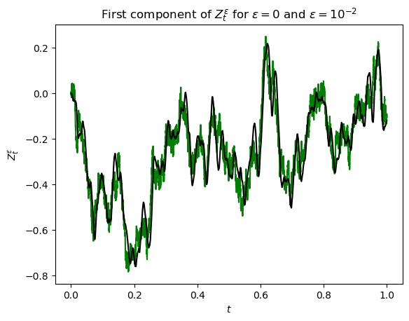
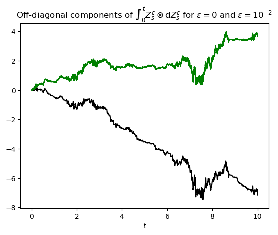
see Section 2.3. In (96) and (97), we allow for both and , that is, we consider the dynamics driven by both mathematical and physical Brownian motion. Note that in the noiseless case our setting coincides with the one discussed in [43, 107], see also Appendix B. Standard arguments show that both and converge in with a nontrivial area correction akin to (94), where in the latter case, refers to the Stratonovich iterated integrals. As an illustration, we plot sample paths of and an off-diagonal component of in Figure 1, comparing the cases and , for the same realisation of (a discretised version of) . Crucially, the convergence towards a nontrivially lifted path as expressed in (94) manifests itself in the offset between the paths in Figure (1(b)), corresponding to a component of in (85). Throughout this section, we choose a fine time step of for all the involved approximations, for the parameter to be recovered, for the strength of the magnetic field, for the variance of the observation noise, and for the drift in (96).
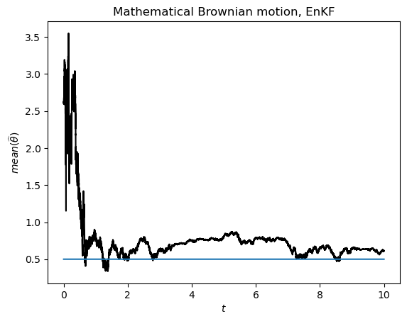
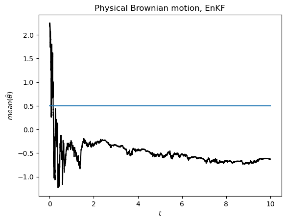
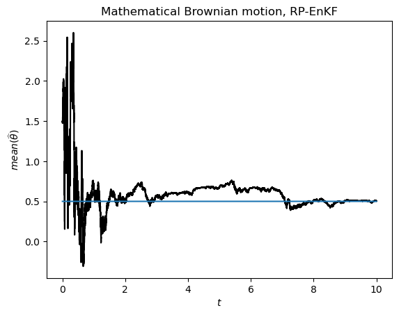
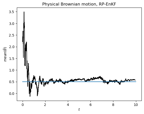
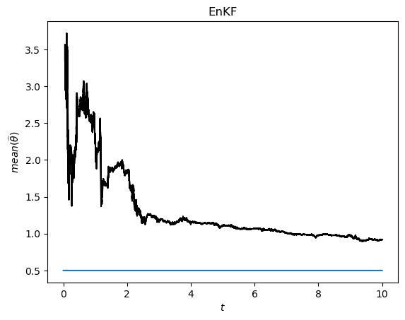
To test the robustness of the EnKF scheme (18) and the RP-EnKF scheme (14), we generate data according to (96) and (97) for both (mathematical Brownian motion) and (physical Brownian motion). We would like to stress that the filtering methodology (expressed in terms of the schemes (18) and (14)) is however based on the model (1) and therefore tailored to the case . In Figure 2, we show the empirical mean of the -components for the output of the EnKF-dynamics (18), considering both mathematical and physical Brownian motion as drivers in (96). Evidently, the EnKF is not robust, in the sense that it fails to recover the true parameter in the case when , see Figure (2(b)).
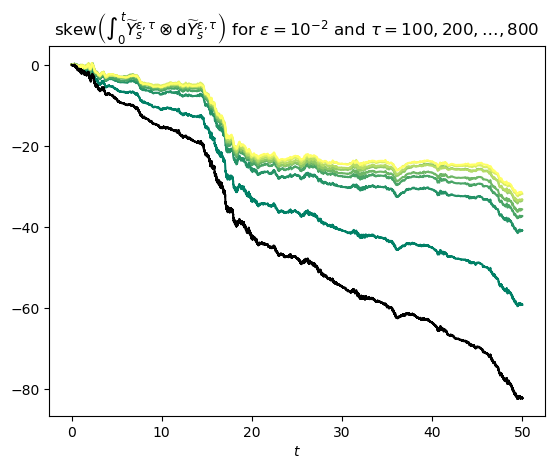
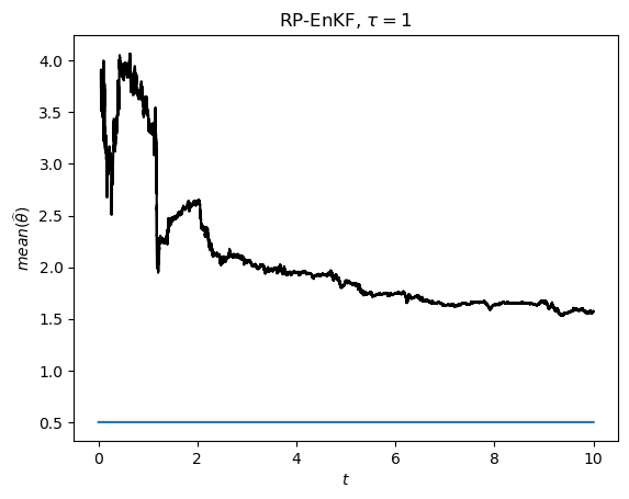
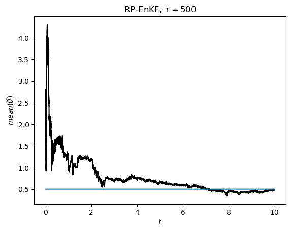
We proceed by showing the corresponding results for the RP-EnKF scheme defined by (77) in Figure 3(b), demonstrating the robustness promised by Theorem 4.17. For the required (discrete-time) lift , we use the construction detailed in Section 6. More precisely, in the case of physical Brownian motion, we set the time-lag to . In the case of mathematical Brownian motion, we set the skew-symmetric part in (81) to zero, , corresponding to the choice . These choices have been made on the basis of the subsampled area processes depicted in Figure 4. More precisely, Figures (4(a)) and (4(c)) show the dependence with different values of the time-lag , for physical Brownian motion (, Figure (4(a))) and mathematical Brownian motion (, Figure (4(c))). While the subsampling only minimally effects the area process associated to the process driven by mathematical Brownian motion (Figure 4(c)), we observe a systematic shift in the case of physical Brownian motion (Figure (4(c))), revealing the latent multiscale structure. The difference between the original and subsampled area processes for physical Brownian motion is shown in Figure (4(b)). As the time-lag increases, said difference approaches the theoretically expected area correction implied by (94)-(95). The fact that the difference between the original and the subsampled area process reaches a plateau at around is illustrated in Figure (4(e)), as opposed to the difference between the original and the subsampled paths, see Figure (4(d)). Consequently, the choice strikes a balance between separating the original and subsampled area processes as much as possible while maintaining similarity between the original and subsampled paths (as suggested by the discussion motivating (90)).
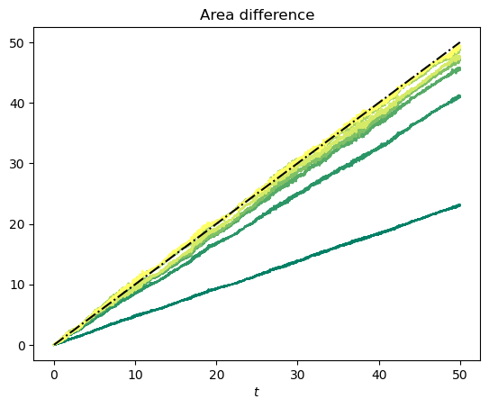

(4(b)): Differences of original and subsampled area processes in the case of physical Brownian motion (), that is , in the spirit of (90). The dashed line represents the theoretically expected area correction according to (94).
(4(c)): Area processes associated to mathematical Brownian motion (), same colour scheme as for Figure (4(a)).
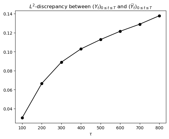
(4(d)): -discrepancy between the original path and the subsampled path as a function of the time-lag for physical Brownian motion ().
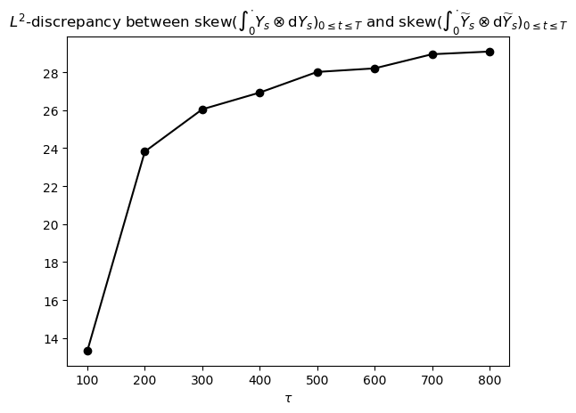
(4(e)): -discrepancy between the original area process and the subsample area process as a function of the time-lag for physical Brownian motion ().
6.2 Fast chaotic dynamics – Lorenz-63
In this example, we consider the rescaled Lorenz ordinary differential equations [110] for ,
| (98a) | |||||
| (98b) | |||||
| (98c) | |||||
with the standard parameters , and as an example of fast chaotic dynamics approximating Brownian noise (with nontrivial area correction). We would like to stress that the phenomena described in this section can be considered generic across a wide range of fast chaotic deterministic dynamical systems, and refer the reader to [20] for an overview.
With , the system (98) has originally been proposed as a simplified model for atmospheric convection [90], and can serve as a prototype for the study of chaotic ODEs. As is well known, (98) possesses a ‘strange’ chaotic attractor equipped with a unique SRB (Sinai-Ruelle-Bowen) measure777The notion of SRB measures provides a suitable generalisation of ergodic measures. , see [120]. For , a random intial condition and after appropriate centering and rescaling, the solution is well approximated by a Brownian motion with a nontrivial area correction in the sense of rough paths:
For Hölder-continuous observables that are -centred (that is, ), a functional CLT (or weak invariance principle) holds for
| (99) |
assuming that is initialised randomly according to . More precisely, there exists a Brownian motion (possibly on an extended probability space) with appropriate covariance such that weakly in as , see [67, Theorem 1.5]888In fact, the convergence takes place -almost surely, see [67, Theorem 1.1]. The covariance is given in terms of suitable long-time ergodic averages or (under certain conditions) Green-Kubo formulae, see [20, 101]. . Moreover, it was shown in [11, Theorem 1.6] that a so-called iterated weak invariance principle holds for the iterated integrals
| (100) |
that is weakly in , where
| (101) |
with area correction . We refer to [20, Theorem 4.4] for the corresponding statement in -variation rough path topology.
In what follows, we consider to be driven by ,
| (102) |
with the parameter to be inferred from noisy observations
| (103) |
and mediating the strength of the chaotic perturbation. Since according to [101, Section Section 11.7.2], we expect (102) to be well approximated by
| (104) |
in the regime , with standard two-dimensional Brownian motion and appropriate covariance . Replacing (102) by (104) is often a desirable simplification both computationally and conceptually, see, for instance, [62], [101, Section 11.7.2], and [115, Section 3.1]. To apply our methodology, we need to presuppose ; estimates can be obtained using the approaches suggested in [62, Example 6.2] or [74], for instance. Here we use the value reported in [74, Section 3.2.6] for and note that almost surely by a short calculation using (98). To test the RP-EnKF, we simulate data according to (98), (102) and (103) using an Euler-Maruyama discretisation with time step , an observation noise level of , a parameter value of to be recovered. Furthermore, we set and . The RP-EnKF is set up according to the model (104) with observations (103), using the scheme (14). As an illustration for the challenges that are posed by the attempt to incorporate data from (102)-(103) into a model of the form (104), we plot the output of the EnKF scheme (18) in Figure (5(a)), noting that it fails to recover the correct parameter value . Figures (5(b)) and (5(c)) show the output of the RP-EnKF scheme (14), with (implying ) and , respectively. We see that the area correction obtained through the subsampling procedure is necessary to obtain satisfactory numerical results. The time-lag has been determined in the same way as in Section 6.1; in particular, plots for the subsampled area processes are qualitatively similar to Figures 4 and 4(b) but are omitted here for the sake of brevity.
6.3 Homogenisation in a two-scale potential
In our final example, we consider the motion of a Brownian particle in a (rugged) two-scale potential,
| (105) |
where , , is an -periodic function in both directions, that is, , for all and , modelling small-scale fluctuations around the potential . It is well known that for , the law of the solution converges weakly in to the law associated to
| (106) |
where , with
| (107) |
see [104] and [101, Chapter 11]. Similar results in a rough-path context can be found in [84]. The homogenised dynamics (106) encapsulates the rugged landscape described by in the diffusion-mass matrix . Like in the previous experiments, we consider the task of estimating the parameter from noisy observations of (105), using the EnKF and RP-EnKF based on (106). We choose , , and . Data from the two-scale dynamics (105) is simulated for , using an Euler-Maruyama discretisation with time step . With the same values for , and , we simulate data from the reduced model (106), where has been obtained by numerical integration in (107). Both (105) and (106) are perturbed by noise according to (103) with and, as in Sections 6.1 and 6.2, the resulting observation paths are used in the EnKF- and RP-EnKF schemes (see equations (18) and (14)) to estimate . We display the results for the means of over time using the EnKF and the RP-EnKF in Figures 6 and 7, respectively.
Clearly, the RP-EnKF deals adequately with multiscale data, while the EnKF fails to recover the true parameter in this setting. We would like to stress that the RP-EnKF scheme has been implemented without area correction, that is imposing as defined in (83). The choice is motivated by a plot analogous and qualitatively similar to Figure 4(c) (omitted due to space considerations), showing that subsampling does not indicate substantial Lévy area correction terms (intuitively, the dynamics (105) does not contain significant ‘rotational’ contributions in the regime ).
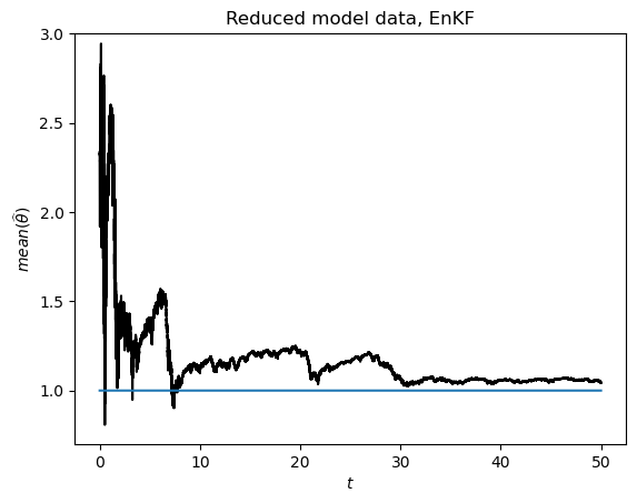
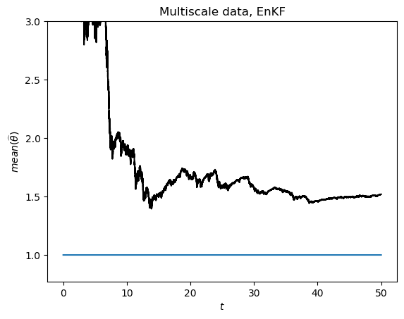
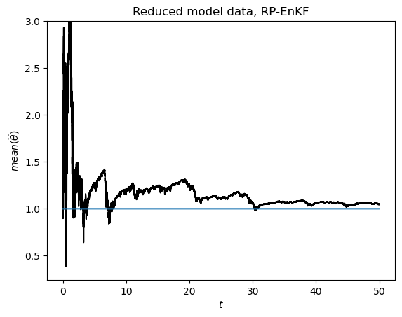
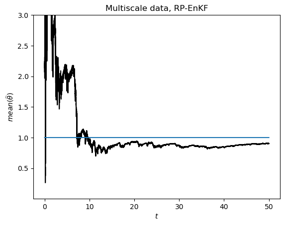
Acknowledgements. This research has been partially funded by Deutsche Forschungsgemeinschaft (DFG) through the grant CRC 1114 ‘Scaling Cascades in Complex Systems’ (project A02, project number 235221301). This work was commenced while T.N. was at TU Berlin, supported by DFG Research Unit FOR2402 “Rough paths and SPDEs” and M.C. was at WIAS Berlin, supported by the Einstein Center Berlin, ECMath Project “Stochastic methods for the analysis of lithium-ion batteries”. We would like to thank R. Chew, A. Djurdjevac, G. Hastermann and R. Klein for very stimulating discussions. N.N. would like to thank M. Engel for organising a seminar on homogenisation at Imperial College London in 2016 leading to Section 6.2, as well as for sharing his insight into the topic.
Appendix A From the filter to the McKean-Vlasov
In this section we prove the formal connection between the filtering problem and the McKean-Vlasov equation. In order to prove Proposition 2.1, we need a few preparations. Let us define
and the likelihood
We can now introduce the unnormalised filtering measures
The measures satisfy the Zakai equation:
Proposition A.1 (Zakai equation).
The evolution of is given by
| (108) |
where
is the generator associated to (1a). The filtering measures can be recovered from the Kalliampur-Striebel formula (or Bayes theorem)
| (109) |
Proof.
This follows from the results in [10, Section 3.8]. ∎
Next, we write the Zakai equation in its Stratonovich form:
Lemma A.2.
The Stratonovich-version of the Zakai equation is given by
Proof.
Using (108), we see that for
where stands for a contribution of finite variation. Recalling , for , we obtain
Similarly, for ,
implying
∎
We now proceed to the proof of Proposition 2.1:
Proof of Proposition 2.1.
Let us define
which is the unnormalised filtering measure associated to (5). Since and are independent given , we have that
From (109) it thus follows that is equivalent to . In the following we therefore compute the evolution of . Notice first that
where, using ,
From we have
implying
| (113a) | ||||
| (113b) | ||||
The last term satisfies
Next, we convert the terms involving and back to their Itô-form,
Here we used the fact that, for every we have and
where . Similarly,
using and, for and ,
We now take the conditional expectation in (113). Note that the conditional expectation w.r.t. commutes with the integration in and that the conditional expectation of the integrals in and vanishes because are independent from , see [26, Appendix B]. We obtain
| (117a) | ||||
| (117b) | ||||
| (117c) | ||||
| (117d) | ||||
Importantly, we have used the fact that and are independent given , and also that and are independent from . The next step is to compare (110) and (117). The -contributions agree if and only if
which we recognise (after identifying and ) to be a weak version of (6).
To compare the -contributions, let us first manipulate the second term in (117c) using (6),
Similarly, the middle term in (117b) satisfies
We now collect terms and compare the -contributions in (110) and (117), arriving at
| (120a) | ||||
| (120b) | ||||
| (120c) | ||||
Next, we work on the first term in (120c),
Plugging this into (120) we see that after a great number of cancellations that (120) reduces to
Using (6) in its weak formulation tested against on the first term in the right-hand side we obtain
| (122) |
which is a weak version of (7).
We have thus obtained constraints on the coefficients of and of the McKean-Vlasov equation (5) such that solves the Zakai equation satisfied by the conditional density of the signal of the filtering problem. We can conclude because the solution to the Zakai equation is assumed to be unique. ∎
Appendix B On the connection between McKean-Vlasov filtering and maximum likelihood estimation
Here we discuss the relationship between parameter estimation based on the ensemble Kalman filter and the maximum likelihood approach considered in [43]. In a nutshell, the two methods essentially agree in the noiseless case with Gaussian initial condition, as relevant McKean-Vlasov dynamics can be solved explicitly in this case. This connection has already been pointed out in [95].
We are given a -dimensional process , which depends on an -dimensional parameter . We observe through the observation , which is possibly noisy.
| (123a) | ||||
| (123b) | ||||
| (123c) | ||||
Here and are independent -dimensional Brownian Motions, is a given function and is a given positive semidefinite deterministic matrix.
Let . We set the -dimensional signal process as and replace the equation for into the equation for the observation . System (123) becomes equivalent to system (1) with the following drift coefficients
Moreover, the coeffiecents of the noise are
Remember is the conditional law of given .
First we consider noiseless observations, i.e. we set . In this case we have that
To convert system (123) to the McKean-Vlasov equation we need to compute as defined in (8), which can be decomposed as follows
In this case with , we have , which implies
We have the following
We have thus obtained explicitly
We now compute , which is defined in (9). We start with the contribution, for , we have
Now compute the contribution in . For and , we have
So that we have
and
If , we have
We can now write the McKean-Vlasov dynamics (11),
| (124a) | ||||
| (124b) | ||||
We interpret equation (124) in the sense of Definition 4.12. Taking expectation in (124b), and writing this equation in integral form, we obtain the rough path maximum likelihood estimator from [43], up to the rescaling , see also [95].
We would like to obtain an equation for the variance of . We start by computing the following equation for the centered random variable ,
By taking the square and using Itô formula we obtain the following equation for
The solution is
Assume now that there exists such that . Since the variance is a path of bounded variation, we have that the integrand in the rough integral in equation (124b) is controlled by in the following way
The Gubinelli derivative is symmetric, which means that the rough integral in (124b) does not depend on the area of the geometric rough path . Hence, the expansion of the integral is completely determined by the path itself.
Appendix C Ito-Stratonovich correction for the Ensemble Kalman filter
In Section 2.4, we derived the system (10) by approximately solving the PDEs (6) and (7). An alternative approach is to convert the Ensemble Kalman filter formulation
| (125) |
from [95] to its Stratonovich form. Here we show that this leads to the same result.
Proof.
Direct calculation (using Itô’s formula for the expression (8) and applying the conditional expectation) shows that
| (127) |
where stands for a process of finite variation. The claim therefore follows from the conversion formula
| (128) |
together with the fact that . ∎
References
- [1] A. Abdulle, G. Garegnani, G. A. Pavliotis, A. M. Stuart, and A. Zanoni. Drift estimation of multiscale diffusions based on filtered data. arXiv preprint arXiv:2009.13457, 2020.
- [2] Y. Ait-Sahalia, P. A. Mykland, and L. Zhang. How often to sample a continuous-time process in the presence of market microstructure noise. The review of financial studies, 18(2):351–416, 2005.
- [3] A. L. Allan. Robust filtering and propagation of uncertainty in hidden Markov models. arXiv preprint arXiv:2005.04982, 2020.
- [4] A. L. Allan, S. N. Cohen, et al. Pathwise stochastic control with applications to robust filtering. Annals of Applied Probability, 30(5):2274–2310, 2020.
- [5] R. Azencott, A. Beri, A. Jain, and I. Timofeyev. Sub-sampling and parametric estimation for multiscale dynamics. Communications in Mathematical Sciences, 11(4):939–970, 2013.
- [6] R. Azencott, A. Beri, and I. Timofeyev. Adaptive sub-sampling for parametric estimation of Gaussian diffusions. Journal of Statistical Physics, 139(6):1066–1089, 2010.
- [7] I. Bailleul, R. Catellier, and F. Delarue. Propagation of chaos for mean field rough differential equations. arXiv preprint arXiv:1907.00578, 2019.
- [8] I. Bailleul, R. Catellier, and F. Delarue. Solving mean field rough differential equations. Electron. J. Probab., 25:Paper No. 21, 51, 2020.
- [9] I. Bailleul and J. Diehl. The inverse problem for rough controlled differential equations. SIAM Journal on Control and Optimization, 53(5):2762–2780, 2015.
- [10] A. Bain and D. Crisan. Fundamentals of stochastic filtering, volume 60. Springer Science & Business Media, 2008.
- [11] P. Bálint and I. Melbourne. Statistical properties for flows with unbounded roof function, including the Lorenz attractor. Journal of Statistical Physics, 172(4):1101–1126, 2018.
- [12] R. Beeson, N. Namachchivaya, and N. Perkowski. Approximation of the filter equation for multiple timescale, correlated, nonlinear systems. arXiv preprint arXiv:2010.16401, 2020.
- [13] R. Beeson, N. Namachchivaya, and N. Perkowski. Quantitative convergence of the filter solution for multiple timescale nonlinear systems with coarse-grain correlated noise. arXiv preprint arXiv:2011.12801, 2020.
- [14] R. Beeson, H. C. Yeong, N. S. Namachchivaya, and N. Perkowski. Reduced order nonlinear filters for multi-scale systems with correlated sensor noise. In 2018 21st International Conference on Information Fusion (FUSION), pages 131–141. IEEE, 2018.
- [15] T. Berry and T. Sauer. Correlation between system and observation errors in data assimilation. Monthly Weather Review, 146(9):2913–2931, 2018.
- [16] A. N. Bishop and P. Del Moral. On the mathematical theory of ensemble (linear-gaussian) Kalman-Bucy filtering. arXiv preprint arXiv:2006.08843, 2020.
- [17] G. Burgers, P. Jan van Leeuwen, and G. Evensen. Analysis scheme in the ensemble Kalman filter. Monthly weather review, 126(6):1719–1724, 1998.
- [18] R. Carmona and F. Delarue. Probabilistic theory of mean field games with applications. II, volume 84 of Probability Theory and Stochastic Modelling. Springer, Cham, 2018. Mean field games with common noise and master equations.
- [19] T. Cass and T. Lyons. Evolving communities with individual preferences. Proc. Lond. Math. Soc. (3), 110(1):83–107, 2015.
- [20] I. Chevyrev, P. K. Friz, A. Korepanov, I. Melbourne, and H. Zhang. Multiscale systems, homogenization, and rough paths. In International Conference in Honor of the 75th Birthday of SRS Varadhan, pages 17–48. Springer, 2016.
- [21] I. Chevyrev and A. Kormilitzin. A primer on the signature method in machine learning. arXiv preprint arXiv:1603.03788, 2016.
- [22] J. Clark. The design of robust approximations to the stochastic differential equations of nonlinear filtering. Communication systems and random process theory, 25:721–734, 1978.
- [23] J. Clark and D. Crisan. On a robust version of the integral representation formula of nonlinear filtering. Probability theory and related fields, 133(1):43–56, 2005.
- [24] M. Coghi, J.-D. Deuschel, P. K. Friz, and M. Maurelli. Pathwise McKean-Vlasov theory with additive noise. Ann. Appl. Probab., 30(5):2355–2392, 2020.
- [25] M. Coghi and F. Flandoli. Propagation of chaos for interacting particles subject to environmental noise. Ann. Appl. Probab., 26(3):1407–1442, 2016.
- [26] M. Coghi and B. Gess. Stochastic nonlinear Fokker–Planck equations. Nonlinear Analysis, 187:259–278, 2019.
- [27] M. Coghi and T. Nilssen. Rough nonlocal diffusions. Stochastic Process. Appl., 141:1–56, 2021.
- [28] C. Cotter, G. Pavliotis, et al. Estimating eddy diffusivities from noisy Lagrangian observations. Communications in Mathematical Sciences, 7(4):805–838, 2009.
- [29] L. Coutin and A. Lejay. Semi-martingales and rough paths theory. Electronic Journal of Probability, 10:761–785, 2005.
- [30] D. Crisan, J. Diehl, P. K. Friz, H. Oberhauser, et al. Robust filtering: correlated noise and multidimensional observation. The Annals of Applied Probability, 23(5):2139–2160, 2013.
- [31] D. Crisan, A. Lobbe, and S. Ortiz-Latorre. Pathwise approximations for the solution of the non-linear filtering problem. arXiv preprint arXiv:2101.03957, 2021.
- [32] D. Crisan and J. Xiong. Approximate McKean–Vlasov representations for a class of SPDEs. Stochastics An International Journal of Probability and Stochastics Processes, 82(1):53–68, 2010.
- [33] A. M. Davie. Differential equations driven by rough paths: an approach via discrete approximation. Applied Mathematics Research eXpress, 2008, 2008.
- [34] M. Davis. On a multiplicative functional transformation arising in nonlinear filtering theory. Zeitschrift für Wahrscheinlichkeitstheorie und verwandte Gebiete, 54(2):125–139, 1980.
- [35] M. Davis and M. Spathopoulos. Pathwise nonlinear filtering for nondegenerate diffusions with noise correlation. SIAM journal on control and optimization, 25(2):260–278, 1987.
- [36] M. H. Davis. A pathwise solution of the equations of nonlinear filtering. Theory of Probability & Its Applications, 27(1):167–175, 1982.
- [37] M. H. Davis. Pathwise nonlinear filtering with correlated noise. The Oxford Handbook of Nonlinear Filtering, pages 403–424, 2011.
- [38] J. de Wiljes, S. Reich, and W. Stannat. Long-time stability and accuracy of the ensemble Kalman–Bucy filter for fully observed processes and small measurement noise. SIAM Journal on Applied Dynamical Systems, 17(2):1152–1181, 2018.
- [39] J. de Wiljes and X. T. Tong. Analysis of a localised nonlinear ensemble Kalman Bucy filter with complete and accurate observations. Nonlinearity, 33(9):4752, 2020.
- [40] P. Del Moral. Feynman-kac formulae. In Feynman-Kac Formulae, pages 47–93. Springer, 2004.
- [41] P. Del Moral, A. Kurtzmann, and J. Tugaut. On the stability and the uniform propagation of chaos of extended ensemble Kalman-Bucy filters. arXiv preprint arXiv:1606.08256, 2016.
- [42] A. Deya, A. Neuenkirch, and S. Tindel. A Milstein-type scheme without Lévy area terms for SDEs driven by fractional Brownian motion. In Annales de l’IHP Probabilités et statistiques, volume 48, pages 518–550, 2012.
- [43] J. Diehl, P. Friz, H. Mai, et al. Pathwise stability of likelihood estimators for diffusions via rough paths. The Annals of Applied Probability, 26(4):2169–2192, 2016.
- [44] J. Diehl, P. K. Friz, and W. Stannat. Stochastic partial differential equations: a rough paths view on weak solutions via Feynman-Kac. Ann. Fac. Sci. Toulouse Math. (6), 26(4):911–947, 2017.
- [45] Z. Ding and Q. Li. Ensemble Kalman inversion: mean-field limit and convergence analysis. Statistics and Computing, 31(1):1–21, 2021.
- [46] Z. Ding, Q. Li, and J. Lu. Ensemble Kalman inversion for nonlinear problems: weights, consistency, and variance bounds. arXiv preprint arXiv:2003.02316, 2020.
- [47] R. L. Dobrušin. Vlasov equations. Funktsional. Anal. i Prilozhen., 13(2):48–58, 96, 1979.
- [48] A. Doucet and A. M. Johansen. A tutorial on particle filtering and smoothing: Fifteen years later. Handbook of nonlinear filtering, 12(656-704):3, 2009.
- [49] A. Duncan, N. Nüsken, and L. Szpruch. On the geometry of stein variational gradient descent. arXiv preprint arXiv:1912.00894, 2019.
- [50] G. Evensen. The ensemble Kalman filter: Theoretical formulation and practical implementation. Ocean dynamics, 53(4):343–367, 2003.
- [51] G. Evensen. Data assimilation: the ensemble Kalman filter. Springer Science & Business Media, 2009.
- [52] G. Flint, B. Hambly, and T. Lyons. Discretely sampled signals and the rough hoff process. Stochastic Processes and their Applications, 126(9):2593–2614, 2016.
- [53] P. Florchinger. Zakai equation of nonlinear filtering with unbounded coefficients. the case of dependent noises. Systems & control letters, 21(5):413–422, 1993.
- [54] N. Fournier and A. Guillin. On the rate of convergence in Wasserstein distance of the empirical measure. Probability Theory and Related Fields, 162(3):707–738, 2015.
- [55] P. Friz, P. Gassiat, and T. Lyons. Physical Brownian motion in a magnetic field as a rough path. Transactions of the American Mathematical Society, 367(11):7939–7955, 2015.
- [56] P. Friz and S. Riedel. Convergence rates for the full Gaussian rough paths. In Annales de l’IHP Probabilités et statistiques, volume 50, pages 154–194, 2014.
- [57] P. K. Friz and M. Hairer. A course on rough paths. Springer, 2020.
- [58] P. K. Friz, A. Hocquet, and K. Lê. Rough stochastic differential equations. arXiv preprint arXiv:2106.10340, 2021.
- [59] P. K. Friz and N. B. Victoir. Multidimensional stochastic processes as rough paths: theory and applications, volume 120. Cambridge University Press, 2010.
- [60] S. Gailus and K. Spiliopoulos. Statistical inference for perturbed multiscale dynamical systems. Stochastic Processes and their Applications, 127(2):419–448, 2017.
- [61] S. Gailus and K. Spiliopoulos. Discrete-time statistical inference for multiscale diffusions. Multiscale Modeling & Simulation, 16(4):1824–1858, 2018.
- [62] D. Givon, R. Kupferman, and A. Stuart. Extracting macroscopic dynamics: model problems and algorithms. Nonlinearity, 17(6):R55, 2004.
- [63] G. A. Gottwald and S. Reich. Supervised learning from noisy observations: Combining machine-learning techniques with data assimilation. arXiv preprint arXiv:2007.07383, 2020.
- [64] I. Gyöngy. On the approximation of stochastic partial differential equations ii. Stochastics: An International Journal of Probability and Stochastic Processes, 26(3):129–164, 1989.
- [65] W. R. Hammersley, D. Šiška, and Ł. Szpruch. Weak existence and uniqueness for McKean–Vlasov SDEs with common noise. The Annals of Probability, 49(2):527–555, 2021.
- [66] A. Hocquet and M. Hofmanová. An energy method for rough partial differential equations. Journal of Differential Equations, 265(4):1407–1466, 2018.
- [67] M. Holland and I. Melbourne. Central limit theorems and invariance principles for Lorenz attractors. Journal of the London Mathematical Society, 76(2):345–364, 2007.
- [68] P. Imkeller, N. S. Namachchivaya, N. Perkowski, and H. C. Yeong. A homogenization approach to multiscale filtering. Procedia IUTAM, 5:34–45, 2012.
- [69] P. Imkeller, N. S. Namachchivaya, N. Perkowski, H. C. Yeong, et al. Dimensional reduction in nonlinear filtering: a homogenization approach. The Annals of Applied Probability, 23(6):2290–2326, 2013.
- [70] S. Kalliadasis, S. Krumscheid, and G. A. Pavliotis. A new framework for extracting coarse-grained models from time series with multiscale structure. Journal of Computational Physics, 296:314–328, 2015.
- [71] D. T. Kelly, K. J. Law, and A. M. Stuart. Well-posedness and accuracy of the ensemble kalman filter in discrete and continuous time. Nonlinearity, 27(10):2579, 2014.
- [72] R. Klein. Scale-dependent models for atmospheric flows. Annual review of fluid mechanics, 42:249–274, 2010.
- [73] P. E. Kloeden and E. Platen. Stochastic differential equations. In Numerical Solution of Stochastic Differential Equations, pages 103–160. Springer, 1992.
- [74] S. Krumscheid, G. A. Pavliotis, and S. Kalliadasis. Semiparametric drift and diffusion estimation for multiscale diffusions. Multiscale Modeling & Simulation, 11(2):442–473, 2013.
- [75] S. Krumscheid, M. Pradas, G. Pavliotis, and S. Kalliadasis. Data-driven coarse graining in action: Modeling and prediction of complex systems. Physical Review E, 92(4):042139, 2015.
- [76] T. G. Kurtz and J. Xiong. Particle representations for a class of nonlinear SPDEs. Stochastic Processes and their Applications, 83(1):103–126, 1999.
- [77] T. G. Kurtz and J. Xiong. Numerical solutions for a class of SPDEs with application to filtering. In Stochastics in finite and infinite dimensions, Trends Math., pages 233–258. Birkhäuser Boston, Boston, MA, 2001.
- [78] H. J. Kushner. A robust discrete state approximation to the optimal nonlinear filter for a diffusion. Stochastics, 3(1-4):75–83, 1980.
- [79] Y. A. Kutoyants. Statistical inference for ergodic diffusion processes. Springer Science & Business Media, 2013.
- [80] T. Lange. Derivation of ensemble Kalman-Bucy filters with unbounded nonlinear coefficients. arXiv preprint arXiv:2012.07572, 2020.
- [81] T. Lange and W. Stannat. On the continuous time limit of ensemble square root filters. arXiv preprint arXiv:1910.12493, 2019.
- [82] T. Lange and W. Stannat. Mean field limit of ensemble square root filters–discrete and continuous time. arXiv preprint arXiv:2011.10516, 2020.
- [83] T. Lange and W. Stannat. On the continuous time limit of the ensemble kalman filter. Mathematics of Computation, 90(327):233–265, 2021.
- [84] A. Lejay and T. Lyons. On the importance of the Lévy area for studying the limits of functions of converging stochastic processes. application to homogenization. In Current trends in potential theory, volume 7. The Theta foundation/American Mathematical Society, 2003.
- [85] T. Lelievre and G. Stoltz. Partial differential equations and stochastic methods in molecular dynamics. Acta Numerica, 25:681, 2016.
- [86] D. Levin, T. Lyons, and H. Ni. Learning from the past, predicting the statistics for the future, learning an evolving system. arXiv preprint arXiv:1309.0260, 2013.
- [87] N. Lingala, N. Perkowski, H. Yeong, N. S. Namachchivaya, and Z. Rapti. Optimal nudging in particle filters. Probabilistic Engineering Mechanics, 37:160–169, 2014.
- [88] N. Lingala, N. Sri Namachchivaya, N. Perkowski, and H. C. Yeong. Particle filtering in high-dimensional chaotic systems. Chaos: An Interdisciplinary Journal of Nonlinear Science, 22(4):047509, 2012.
- [89] R. S. Liptser and A. N. Shiryaev. Statistics of random processes II: Applications, volume 6. Springer Science & Business Media, 2013.
- [90] E. N. Lorenz. Deterministic nonperiodic flow. Journal of atmospheric sciences, 20(2):130–141, 1963.
- [91] T. Lyons. Rough paths, signatures and the modelling of functions on streams. arXiv preprint arXiv:1405.4537, 2014.
- [92] H. P. McKean, Jr. A class of Markov processes associated with nonlinear parabolic equations. Proc. Nat. Acad. Sci. U.S.A., 56:1907–1911, 1966.
- [93] J. Nolen, G. A. Pavliotis, and A. M. Stuart. Multiscale modelling and inverse problems. In Numerical analysis of multiscale problems, pages 1–34. Springer, 2012.
- [94] N. Nüsken. Stein optimal transport for Bayesian inference.
- [95] N. Nüsken, S. Reich, and P. J. Rozdeba. State and parameter estimation from observed signal increments. Entropy, 21(5):505, 2019.
- [96] N. Nüsken and D. Renger. Stein variational gradient descent: many-particle and long-time asymptotics. arXiv preprint arXiv:2102.12956, 2021.
- [97] S. C. Olhede, A. M. Sykulski, and G. A. Pavliotis. Frequency domain estimation of integrated volatility for Itô processes in the presence of market-microstructure noise. Multiscale Modeling & Simulation, 8(2):393–427, 2010.
- [98] A. Papavasiliou, G. Pavliotis, and A. Stuart. Maximum likelihood drift estimation for multiscale diffusions. Stochastic Processes and their Applications, 119(10):3173–3210, 2009.
- [99] S. Pathiraja, S. Reich, and W. Stannat. McKean-Vlasov SDEs in nonlinear filtering. arXiv preprint arXiv:2007.12658, 2020.
- [100] S. Pathiraja and W. Stannat. Analysis of the feedback particle filter with diffusion map based approximation of the gain. 2021.
- [101] G. Pavliotis and A. Stuart. Multiscale methods: averaging and homogenization. Springer Science & Business Media, 2008.
- [102] G. A. Pavliotis. Stochastic processes and applications: Diffusion Processes, the Fokker-Planck and Langevin Equations, volume 60. Springer, 2014.
- [103] G. A. Pavliotis, Y. Pokern, and A. M. Stuart. Parameter estimation for multiscale diffusions: an overview. In Statistical methods for stochastic differential equations, volume 124 of Monogr. Statist. Appl. Probab., pages 429–472. CRC Press, Boca Raton, FL, 2012.
- [104] G. A. Pavliotis and A. Stuart. Parameter estimation for multiscale diffusions. Journal of Statistical Physics, 127(4):741–781, 2007.
- [105] J. Pidstrigach and S. Reich. Affine-invariant ensemble transform methods for logistic regression. arXiv preprint arXiv:2104.08061, 2021.
- [106] S. Reich. Data assimilation: the Schrödinger perspective. Acta Numerica, 28:635–711, 2019.
- [107] S. Reich. Frequentist perspective on robust parameter estimation using the ensemble Kalman filter. arXiv preprint arXiv:2201.00611, 2022.
- [108] S. Reich and C. Cotter. Probabilistic forecasting and Bayesian data assimilation. Cambridge University Press, 2015.
- [109] D. Simon. Optimal state estimation: Kalman, H infinity, and nonlinear approaches. John Wiley & Sons, 2006.
- [110] C. Sparrow. The Lorenz equations. Edited by Arun V. Holden, page 111, 1982.
- [111] A.-S. Sznitman. Topics in propagation of chaos. In École d’Été de Probabilités de Saint-Flour XIX—1989, volume 1464 of Lecture Notes in Math., pages 165–251. Springer, Berlin, 1991.
- [112] A. Taghvaei, J. De Wiljes, P. G. Mehta, and S. Reich. Kalman filter and its modern extensions for the continuous-time nonlinear filtering problem. Journal of Dynamic Systems, Measurement, and Control, 140(3), 2018.
- [113] A. Taghvaei, P. G. Mehta, and S. P. Meyn. Diffusion map-based algorithm for gain function approximation in the feedback particle filter. SIAM/ASA Journal on Uncertainty Quantification, 8(3):1090–1117, 2020.
- [114] H. Tanaka. Limit theorems for certain diffusion processes with interaction. In Stochastic analysis (Katata/Kyoto, 1982), volume 32 of North-Holland Math. Library, pages 469–488. North-Holland, Amsterdam, 1984.
- [115] J. Wouters and G. A. Gottwald. Stochastic model reduction for slow-fast systems with moderate time scale separation. Multiscale Modeling & Simulation, 17(4):1172–1188, 2019.
- [116] T. Yang, P. G. Mehta, and S. P. Meyn. Feedback particle filter. IEEE transactions on Automatic control, 58(10):2465–2480, 2013.
- [117] H. C. Yeong, R. Beeson, N. S. Namachchivaya, N. Perkowski, and P. W. Sauer. Dynamic data-driven adaptive observations in data assimilation for multi-scale systems. In Handbook of Dynamic Data Driven Applications Systems, pages 47–73. Springer, 2018.
- [118] H. C. Yeong, R. T. Beeson, N. S. Namachchivaya, and N. Perkowski. Particle filters with nudging in multiscale chaotic systems: with application to the Lorenz-96 atmospheric model. Journal of Nonlinear Science, pages 1–34, 2020.
- [119] Y. Ying, J. Maddison, and J. Vanneste. Bayesian inference of ocean diffusivity from Lagrangian trajectory data. Ocean Modelling, 140:101401, 2019.
- [120] L.-S. Young. What are SRB measures, and which dynamical systems have them? Journal of statistical physics, 108(5):733–754, 2002.
- [121] L. Zhang, P. A. Mykland, and Y. Aït-Sahalia. A tale of two time scales: Determining integrated volatility with noisy high-frequency data. Journal of the American Statistical Association, 100(472):1394–1411, 2005.