Linear stability of a rotating liquid column revisited

Abstract

We revisit the somewhat classical problem of the linear stability of a rigidly rotating liquid column in this communication. Although literature pertaining to this problem dates back to 1959, the relation between inviscid and viscous stability criteria has not yet been clarified. While the viscous criterion for stability, given by $We<n^{2}+k^{2}-1$, is both necessary and sufficient, this relation has only been shown to be sufficient in the inviscid case. Here, $We=\rho\Omega^{2}a^{3}/\gamma$ is the Weber number and measures the relative magnitudes of the centrifugal and surface tension forces, with $\Omega$ being the angular velocity of the rigidly rotating column, $a$ the column radius, $\rho$ the density of the fluid, and $\gamma$ the surface tension coefficient; $k$ and $n$ denote the axial and azimuthal wavenumbers of the imposed perturbation. We show that the subtle difference between the inviscid and viscous criteria arises from the surprisingly complicated picture of inviscid stability in the $We-k$ plane. For all $n>1$, the viscously unstable region, corresponding to $We>n^{2}+k^{2}-1$, contains an infinite hierarchy of inviscidly stable islands ending in cusps, with a dominant leading island. Only the dominant island, now infinite in extent along the $We$ axis, persists for $n=1$. This picture may be understood, based on the underlying eigenspectrum, as arising from the cascade of coalescences between a retrograde mode, that is the continuation of the cograde surface-tension-driven mode across the zero Doppler frequency point, and successive retrograde Coriolis modes constituting an infinite hierarchy.

1 Introduction

This article discusses the linear stability of a rigidly rotating liquid column. The limit of zero rotation corresponds to the classical Rayleigh-Plateau problem analyzed first, in the inviscid limit, by Plateau (1873) and later by Rayleigh (1878). The subsequent literature on the rigidly rotating liquid column [Hocking & Michael (1959); Hocking (1960); Gillis & Kaufman (1962); Pedley (1967)] primarily focused on the necessary and/or sufficient condition for instability, although later Weidman et al. (1997) examined the dominant unstable modes for the inviscid rotating column based on growth-rate calculations. More recently, Kubitschek & Weidman (2007a) obtained the dominant modes for the viscous rotating column, and organized their results based on the wavenumber of the dominant perturbation, in a parameter plane consisting of the Weber number (a dimensionless measure of rotation defined below) and the column Reynolds number. The boundaries demarcating the crossover of the dominant mode in this plane converged smoothly to the inviscid predictions of Weidman et al. (1997) for $Re\to\infty$. The later experiments of Kubitschek & Weidman (2007b) were consistent with the modal crossover boundaries obtained in Kubitschek & Weidman (2007a). While all of the above results show the expected destabilizing effect of rotation, in terms of a larger range of wavenumbers turning unstable with an increase in the column angular velocity, on account of centrifugal forces, there remains a difference between the viscous and inviscid criteria for instability obtained in the early literature [Hocking & Michael (1959); Hocking (1960); Gillis & Kaufman (1962); Pedley (1967)]. Although the expression for the stability threshold (see eq. 6 below) remains the same in both cases, it has been shown to be necessary and sufficient in the presence of viscosity [Gillis & Kaufman (1962)], but only serves as a sufficient condition in the inviscid limit [Pedley (1967); Weidman (1994); Henderson & Barenghi (2002)]. In this article, we re-examine the instability of a rigidly rotating liquid column, with an emphasis on the entire inviscid spectrum, including the neutral modes. The analysis sheds new light on this problem, showing that inviscid unstable modes arise from an infinite hierarchy of coalescences between pairs of dispersion curves just above the viscous threshold. The resulting intricate picture helps explain the aforementioned difference between the nature of the inviscid and viscous threshold criteria.

Perturbations to a liquid column may be characterized in terms of their azimuthal $(n)$ and axial $(k)$ wavenumbers, and accordingly, may be classified as axisymmetric ($n=0,k\neq 0$), planar ($n\neq 0,k=0$), and helical (spiral) or three-dimensional perturbations ($n\neq 0,k\neq 0$). Starting in section 2, we study the dispersion curves, and the associated stability thresholds, for a rigidly rotating column of liquid subject to each of the aforementioned classes of perturbations. The nature of the dispersion curves is a function of the Weber number, $We=\rho\Omega^{2}a^{3}/\gamma$, a dimensionless parameter that compares the relative importance of centrifugal and surface tension forces; here, $\rho$ is the density, $\Omega$ the column angular velocity, $a$ the column radius, and $\gamma$ the coefficient of surface tension. For helical perturbations, we analyze the dispersion curves in the $We-k$ plane for different fixed $n$’s. Note that, following early work by Hocking [Hocking & Michael (1959); Hocking (1960)], $We^{-1}$ has often been referred to as the Hocking parameter ($L$); for instance, the aforementioned efforts of Weidman et al. (1997) and Kubitschek & Weidman (2007a) presented their results for the dominant inviscid modes as a function of $L$, and the dominant viscous modes in the $L-Re$ plane, respectively. In what follows, we stick to $We$. In the next paragraph, we begin by recapitulating the well known results for the classical case of a stationary liquid column ($We=0$).

The classical Rayleigh-Plateau instability is one of a stationary liquid column to sufficiently long wavelength axisymmetric perturbations, and explains the spontaneous breakup of a (slow) jet into nearly uniformly sized droplets (see Chandrasekhar (1981); for sufficiently slow speeds, the shear at the air-water interface is unimportant, and the jet may be made equivalent to a stationary column via a Galilean transformation). Plateau (1873) concluded, via a quasi-static analysis, that perturbations with an axial wavelength greater than the circumference of the column ($ka<1$ or, if the wavenumber is scaled with the column radius, $k<1$) act to destabilize the column by decreasing the total interfacial area. Rayleigh (1878) then accounted for both inertia and surface tension, obtaining the following dispersion relation for small amplitude Fourier mode perturbations, proportional to $e^{i(kx+n\theta-\sigma t)}$, in the inviscid limit

$$\sigma^{2}=k\frac{I_{n}^{\prime}(k)}{I_{n}(k)}(k^{2}+n^{2}-1),$$ (1)

where $\sigma=\sigma_{r}+i\sigma_{i}$ has been scaled with $\sqrt{\gamma/\rho a^{3}}$ ($\sigma_{r}$ being the frequency and $\sigma_{i}$ being the growth rate), and the axial wavenumber $(k)$ is now scaled with $1/a$; $I_{n}(k)$ is the modified Bessel function of the first kind with the prime denoting differentiation. From (1.1), only axisymmetric perturbations are found to be unstable ($\sigma_{i}>0$) for $k<1$, with the maximum growth rate corresponding to $k=0.697$. The growing and decaying modes transform to a pair of neutral modes across $k=1$, the latter corresponding to capillary waves propagating in opposite directions along the axis of the column. For $k\rightarrow\infty$, one obtains $\sigma=\sqrt{\gamma k^{3}/\rho}$ regardless of $n$, which is the dispersion relation for capillary waves propagating on an infinite plane interface.

Hocking & Michael (1959) and Hocking (1960) first investigated the effects of rotation on a liquid column subject to planar and axisymmetric perturbations, obtaining the necessary and sufficient criteria for stability. For the axisymmetric case, the authors obtained the criterion $We<k^{2}-1$, regardless of viscosity. For the planar case, the authors found the inviscid criterion to be $We<n(n+1)$, while that for any finite viscosity to be $We<n^{2}-1$ (see also Gillis (1961)). Gillis & Kaufman (1962) later studied three-dimensional perturbations of a viscous rotating column and concluded that the latter criterion generalizes to $We<k^{2}+n^{2}-1$. Pedley (1967) showed that although the aforementioned viscous criterion remains relevant in the inviscid limit, it only serves as a sufficient condition for stability. Thus, for inviscid columns, a necessary and sufficient condition is not yet known, and clarifying the above difference between the viscous and inviscid criteria is the subject of this effort. As stated above, our focus on the entire eigenspectrum allows us to understand in detail the regions in parameter space corresponding to the inviscid unstable modes while also pointing to the necessary and sufficient criterion for inviscid stability.

While the main findings of the present effort pertain to helical perturbations, we nevertheless consider all three classes of perturbations mentioned above, in sequence, and a complete picture of linear stability emerges as a consequence. Thus, section 2 below starts off with a brief description of the linear stability formulation, which is then followed by subsections pertaining to axisymmetric (section 2.1) and planar (section 2.2) perturbations. We detail our new findings for three-dimensional perturbations in section 2.3. In the conclusions section (section 3), we show that our findings with regard to the non-trivial nature of the inviscid spectrum carry over to the case where the interfacial cohesion underlying surface tension is replaced by a volumetric cohesion mechanism, that of self-gravitation, instead. This makes our findings relevant to the astrophysical scenario, and we end with a few pertinent comments in this regard.

2 The Rotating Liquid Column

The rigidly rotating columnar base state corresponds to $u_{r}=0$, $u_{\theta}=\Omega r$, $u_{z}=0,$ and $p=p_{0}+\frac{\rho\Omega^{2}r^{2}}{2}$ for $r<a$, where $p_{o}$ is an arbitrary baseline pressure on account of incompressibility. The governing linearized equations for small-amplitude perturbations may be derived in the usual way from the Euler equations, with kinematic (radial velocity) and dynamic (pressure) boundary conditions at the column free surface. The equations governing inviscid evolution have already been written down and solved in earlier efforts [Hocking & Michael (1959); Hocking (1960); Weidman et al. (1997)], and in what follows, we directly examine the resulting dispersion relations. Note that the density of the exterior fluid is assumed to be small relative to that of the liquid column, and its influence on column oscillations is neglected.

2.1 Axisymmetric Perturbations

The dispersion relation for axisymmetric perturbations was obtained by Hocking (1960), and is given by

$$We\;\sigma^{2}\sqrt{\frac{4}{\sigma^{2}}-1}\frac{J_{0}(\alpha)}{J_{1}(\alpha)}-k\left(k^{2}-1\right)+We\;k=0,$$ (2)

where $\alpha=k\sqrt{\frac{4}{\sigma^{2}}-1}$. Here, as before, $k$ is scaled with $1/a$ but $\sigma$ is scaled with $\Omega$ as opposed to $\sqrt{\gamma k^{3}/\rho}$ used in eq. 1. Using eq. 2, Hocking obtained the necessary and sufficient criterion for stability to be

$$We<k^{2}-1$$ (3)

indicating that centrifugal forces destabilize the system, increasing the interval of unstable wavenumbers from $(0,1)$ in the non-rotating case to $(0,\sqrt{1+We})$ in the rotating case.

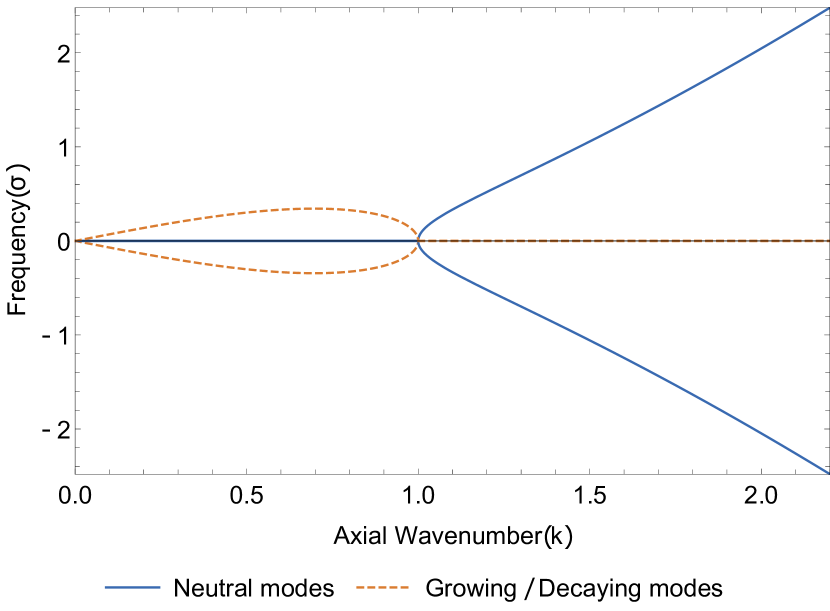
(a) Rayleigh-Plateau problem

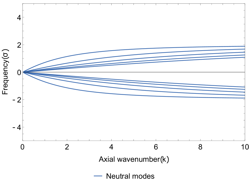
(b) Rankine vortex

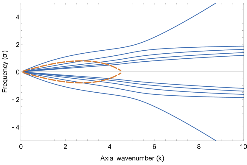
(c) Rotating liquid column

Figure 1: The dispersion curves for the Rayleigh-Plateau problem (top-left), the Rankine vortex (top-right) and the rotating liquid column with $We=20$ (bottom). Blue curves denote neutral modes while the dotted orange curves denote growing/decaying modes. Only the first ten of the infinite number of neutral modes are shown for the Rankine vortex and the rotating column.

Fig. 1(c) shows the dispersion curves for the axisymmetrically perturbed column obtained from eq. 2. The spectrum is seen to borrow its traits from two constituent cases - the Rayleigh-Plateau configuration involving only surface tension (Fig. 1(a)) and the Rankine vortex involving only rotation (Fig. 1(b)). Much like the Rankine vortex, the rotating liquid column supports an infinite sequence of primarily Coriolis-force-driven modes (henceforth referred to as the Coriolis modes), with the inner dispersion curves corresponding to perturbations with an increasingly fine-scaled radial structure; note that the Rankine vortex has recently been shown to also possess a continuous spectrum on account of the irrotational shear in the column exterior [Roy & Subramanian (2014), Roy et al. (2021)]. The Coriolis modes in both these problems have frequencies $\sigma_{r}\in(-2,2)$. Additionally, the rotating liquid column has two modes that owe their origin to surface tension akin to the Rayleigh-Plateau configuration (henceforth referred to as the capillary modes). Fig. 1(c) shows the family of Coriolis modes along with the two capillary modes, and their variation with $k$, for $We=20$. Note that the pair of capillary modes follow the characteristic $k^{3/2}$ scaling for large $k$, while the Coriolis mode frequencies approach $\sigma_{r}=\pm 2$ in this limit. The effect of $We$ on the dispersion curves is illustrated in Fig. 2. For $k\ll\sqrt{We+1}$, Coriolis forces dominate the spectrum, and it is only for $k>\sqrt{We+1}$ that the effects of surface tension become apparent, with the pair of capillary mode dispersion curves transitioning to the aforementioned $k^{3/2}$ scaling. For $We\gg k^{2}-1$, eq. 2 reduces to $\sigma^{2}\sqrt{\frac{4}{\sigma^{2}}-1}\frac{J_{0}(\alpha)}{J_{1}(\alpha)}+k=0$, a $We$-independent dispersion relation; the transition $k$ has receded to infinity and the entire spectrum is governed by Coriolis forces.

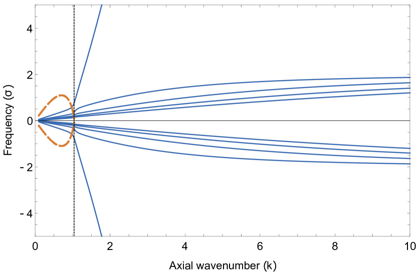
(a) $We=0.1$

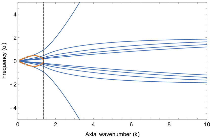
(b) $We=1$

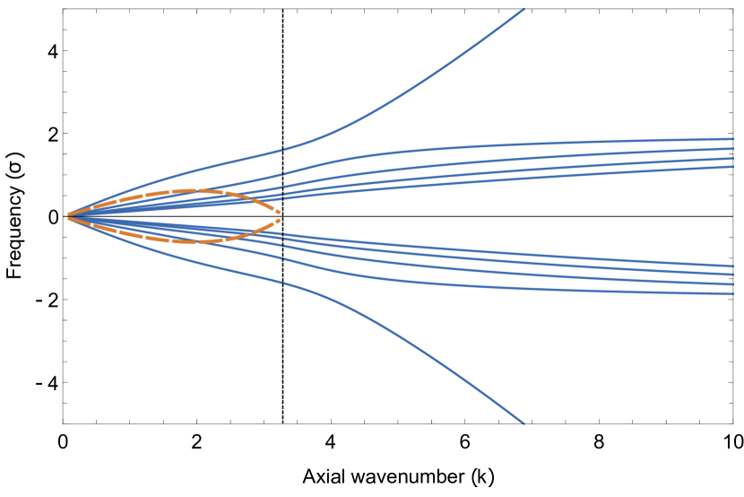
(c) $We=10$

(d) $We=20$

Figure 2: The dispersion curves of the rotating liquid column with varying $We$. Blue curves denote neutral modes while dashed orange curves denote growing / decaying modes. A vertical dashed line drawn at $k=\sqrt{1+We}$ indicates the axial wavenumber beyond which the effects of surface tension on the neutral modes become significant.

The description above clearly shows that there is a qualitative change in the nature of the eigenspectrum with the onset of rotation, as evident from comparing Figs. 1(a) and 1(c), and points to the stationary column $(We\rightarrow 0)$ being a singular limiting case. The interfacial dynamics for the stationary column is entirely determined by the pair of capillary modes (whether neutral or unstable), which are now irrotational. For these modes, the non-dimensional frequency ($\sigma$) in eq. 2 diverges in the limit of zero rotation. Thus, $\alpha$ reduces to $ik$ and one recovers the Rayleigh-Plateau dispersion relation given in eq. 1. In contrast, the Coriolis modes, which remain vortical in the zero-rotation limit, may be regarded as a complete set of stationary vortical perturbations that do not perturb the column free surface. For these modes, the non-dimensional frequency $\sigma$ remains finite (implying that the dimensional one vanishes as $O(\Omega)$), and therefore, so does $\alpha$. The dispersion relation reduces to $\mathit{We}\,J_{0}(\alpha)/J_{1}(\alpha)=k(k^{2}-1)$, implying that $J_{1}(\alpha)=0$ governs the Coriolis mode frequencies for $We=0$; this also ensures that the radial velocity vanishes at $r=1$ (see eq. 3.2a in Kubitschek & Weidman (2007a)), consistent with the aforementioned requirement of an unperturbed free surface. An analogous limiting scenario prevails for any non-zero $n$, with the limiting dispersion relation being given by $\sigma-n=\frac{2n\,J_{n}(\alpha)}{\alpha J_{n}^{\prime}(\alpha)}$; thus, the Coriolis modes, in all cases, reduce to stationary vortical perturbations as $We\rightarrow 0$, and are irrelevant to the dynamics of free surface disturbances.

Finally, it needs mentioning that while the growing and decaying modes for the rotating column exist over a wider range of wavenumbers given by $0<k<\sqrt{1+We}$, they do not emerge as a result of coalescence of neutral modes, as was the case for the Rayleigh-Plateau problem (where the so-called ‘principle of exchange of stability’ holds); instead, as evident from the dashed dispersion curves in Figs. 1 and 2, they arise independently as the stability threshold is crossed. Importantly, since the eigenvalues associated with these modes are purely imaginary, the state of neutral stability is one of rigid rotation, and therefore, as pointed out by Rosenthal (1962), viscosity cannot alter the threshold. Thus, $We=k^{2}-1$ remains the threshold regardless of the column Reynolds number (which may be defined as $Re=\Omega a^{2}/\nu$, $\nu$ being the kinematic viscosity).

2.2 Planar Perturbations

Next, we examine planar perturbations, the inviscid dispersion relation for which was first obtained by Hocking & Michael (1959) and is given by

$$\sigma=n-1\pm\sqrt{\frac{(n-1)(n(n+1)-We)}{We}},$$ (4)

which is algebraic (quadratic) instead of transcendental, as was the case for axisymmetric perturbations (see eq. 2), and as is also the case for helical perturbations (see eq. 7). The existence of only a pair of planar modes is because the infinite number of Coriolis modes degenerate to $\sigma=n$ for $k\rightarrow 0$ in the inviscid limit; see Figs 1(c) and 4(a). For any $We$, the two planar-wave frequencies are symmetrically distributed about $n-1$. For small $We$, they are asymptotically large (of $O(We^{-1/2})$, which corresponds to a dimensional frequency of $\sqrt{\gamma/\rho a^{3}}$, as expected, and approach each other with increasing $We$. For $n\geq 2$, the modes coalesce at $\sigma=n-1$ for $We=n(n+1)$, the inviscid threshold mentioned earlier, and become complex valued for $We>n(n+1)$, implying instability.

Unlike the axisymmetric case, viscosity has a profound effect on the stability of the rotating column to planar perturbations. To see this, let $\Lambda=\frac{n(n^{2}-1)}{We}-n$ so that the pair of inviscid frequencies above may be written as $\sigma=n-1\pm\sqrt{1+\Lambda}$ and the inviscid threshold corresponds to $\Lambda=-1$. For large but finite $Re$, Hocking (1960) obtained the following expressions for the planar-wave frequencies, corrected for viscous effects, again as the solutions of a quadratic equation

$$\sigma=n-1\pm\sqrt{1+\Lambda}-\frac{i}{Re}\left(2n(n-1)\frac{-1\pm\sqrt{1+\Lambda}}{\pm\sqrt{1+\Lambda}}\right).$$ (5)

Note that the $O(1/Re)$ scaling for the viscous correction, implied by eq. 5, is not valid near the inviscid threshold as the expression within brackets diverges for $\Lambda\to-1$. One may nevertheless derive the requirement for viscous instability. This corresponds to $\sigma$ in eq. 5 having a negative imaginary part which in turn translates to $\Lambda=0$ (bounded away from the aforementioned breakdown value), or $We=n^{2}-1$. This threshold was shown to be applicable for columns of all finite $Re$ [Gillis (1961)]. Rather counterintuitively, on one hand, the viscous threshold does not depend on $Re$, leading to the aforementioned discontinuous jump in the threshold $We$ from $n(n+1)$ to $n^{2}-1$. On the other hand, the viscous threshold for stability is less than the inviscid threshold, implying the destabilizing influence of viscosity. The latter behavior is attributed to the phase difference between pressure and displacement waves. The two waves are exactly out of phase in the inviscid limit. This is no longer true in presence of viscous effects which allow for a net work done during a single oscillation. The role of viscosity in modifying the phase difference, and thereby inducing exponential growth, is reminiscent of the Miles mechanism that accounts for the growth of wind-driven gravity waves [Miles (1957); Benjamin (1959)]; although, on account of the rigidly rotating base state, there isn’t the complicating effect of a critical layer [Miles (1957)] in the present problem.

Figs. 3(a) and 3(b) show that although the stability threshold changes discontinuously for any finite $Re$, the growth rates in the interval between the inviscid and viscous thresholds ($n^{2}-1<We<n(n+1)$) scale viscously, and therefore, decrease to zero for $Re\rightarrow\infty$ (see also the figure in Gillis (1961) and Fig. 6c in Kubitschek & Weidman (2007a)). For $We\in(n^{2}-1,n(n+1))$, the growth rates scale as $Re^{-1}$, while remaining $O(1)$ for $We>n(n+1)$. Within a small $O(Re^{-2})$ interval around $We=n(n+1)$, the growth rates exhibit a slower decay of $O(Re^{-1/2})$ for $Re\rightarrow\infty$, consistent with the singular role of viscosity in the neighborhood of the inviscid threshold, implied by eq. 5; see Fig. 3(b). Finally, it is worth mentioning that the viscous dispersion relation is a transcendental one even for planar modes [Hocking (1960)]. Thus, for any finite $Re$, there exist an infinite number of planar modes, and importantly, they remain non-degenerate. It may be shown that all but two of these modes (the two being governed by the corrected quadratic derived by Hocking, given by eq. 5) have $\sigma_{r}\rightarrow n\Omega$, with $\sigma_{i}\sim O(Re^{-1})$ in the limit $Re\rightarrow\infty$. The zero Doppler frequency limit $(\sigma_{r}-n\Omega=0)$ suggests that these remaining modes correspond to the limiting forms of the planar Coriolis modes for large but finite $Re$. In fact, for any finite $Re$, the $\sigma_{i}$’s for the Coriolis modes form an infinite sequence asymptoting to $-\infty$ with increasing modal index, this being consistent with the fact that the finer-scaled modes must exhibit progressively greater (viscous) decay rates.

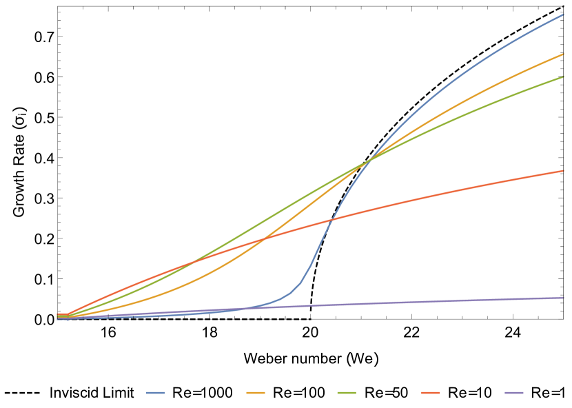
(a) Growth rates vs $We$ for various $Re$.

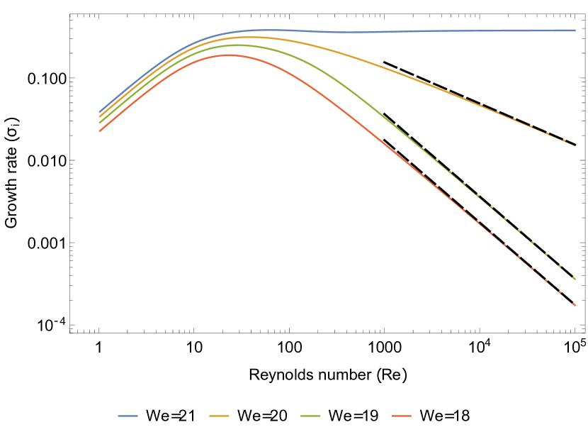
(b) Growth rates vs $Re$ for various $We$.

Figure 3: The two figures plot the growth rates of planar perturbations as a function of $We$ and $Re$, respectively, for $n=4$. Note the discontinuous change in the stability criterion from $We=20$, for the inviscid case (the dotted black curve in (a)) to $We=15$ for any finite $Re$. Dashed black lines in (b) denote the large $Re$ asymptotes obtained from the planar viscous dispersion relation due to Hocking (1960).

2.3 Three-dimensional Perturbations

The effect of rotation on three-dimensional perturbations is well understood only in the presence of viscosity. As shown first by Gillis & Kaufman (1962), the necessary and sufficient criterion for the stability of the rotating column in the presence of viscosity is

$$We<k^{2}+n^{2}-1.$$ (6)

It is easily seen that eq. 6 reduces to the corresponding criteria for viscous planar and axisymmetric perturbations for $n=0$ and $k=0$, respectively. For inviscid stability, however, this criterion has only been shown to be a sufficient one [Pedley (1967)]. The relevance of the same threshold $We(=k^{2}+n^{2}-1)$ in the presence and absence of viscosity is because, as will be seen below, similar to the axisymmetric case, the system is in a state of rigid-body rotation at this $We$. However, the change from a necessary and sufficient condition in the viscous case to only a sufficient one in the inviscid limit points to the possibly subtle relation between the inviscid and viscous stability scenarios.

The dispersion relation for the inviscid rotating column has, in fact, already been given by Weidman et al. (1997) as

$$\alpha\frac{J_{n-1}(\alpha)}{J_{n}(\alpha)}-\frac{We\left(4-(\sigma-n)^{2}\right)}{We+1-n^{2}-k^{2}}-n\left(1+\frac{2}{(\sigma-n)}\right)=0,$$ (7)

where $\alpha=k\sqrt{\frac{4}{(\sigma-n)^{2}}-1}$. It will be shown below that, for a given $n>1$, the spectrum as governed by eq. 7 changes qualitatively with increasing $We$. This is illustrated in Fig. 4 which shows four sets of dispersion curves, for $n=3$, each corresponding to a different regime.

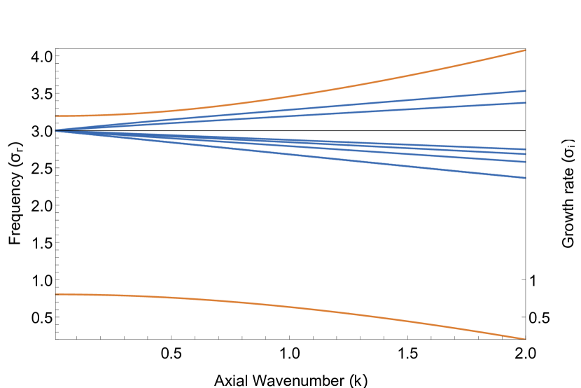
(a) $We=7$

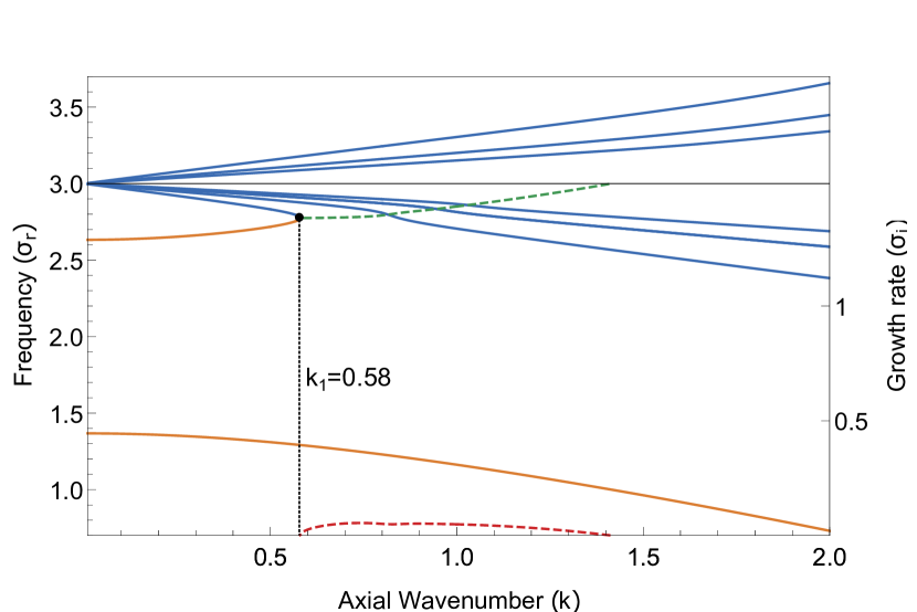
(b) $We=10$

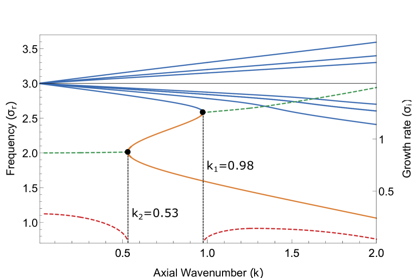
(c) $We=12.5$

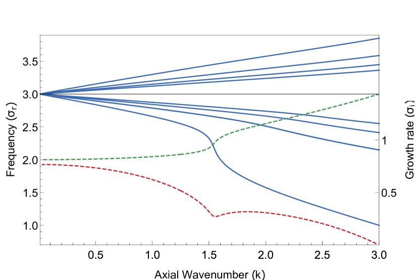
(d) $We=17$

Figure 4: The inviscid dispersion curves corresponding to the different $We$-regimes for $n=3$: (a) $We<n^{2}-1$ (b) $n^{2}-1<We<n(n+1)$, (c) $n(n+1)<We<We_{\text{cusp}}$ and (d) $We>We_{\text{cusp}}$; $We_{\text{cusp}}\approx 16$ for $n=3$. The neutral Coriolis modes are shown in blue and the neutral capillary modes in orange. The real part of the unstable eigenvalues are shown as dashed green curves while the imaginary parts are shown as dashed red curves.

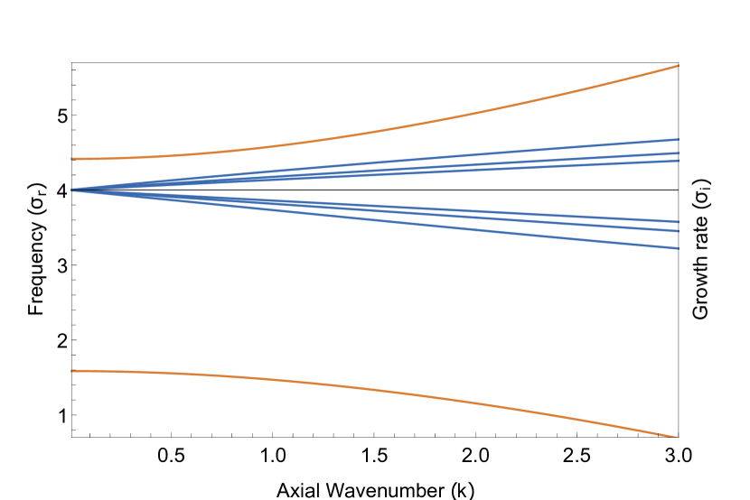
(a) $We=12$

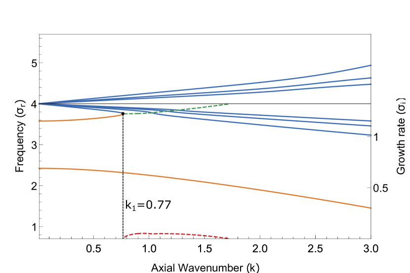
(b) $We=18$

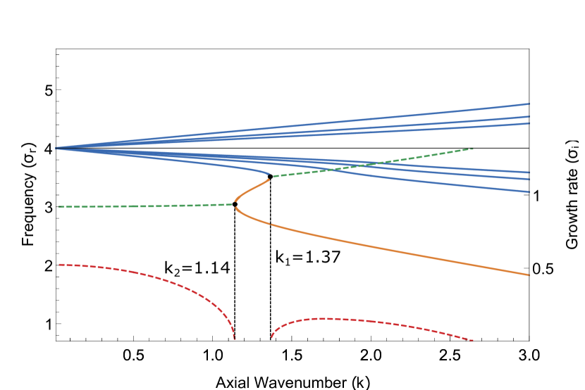
(c) $We=22$

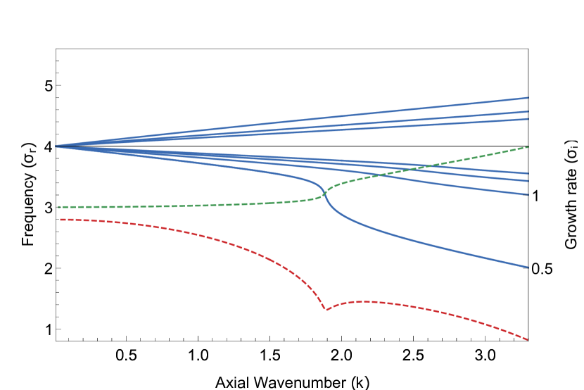
(d) $We=26$

Figure 5: The inviscid dispersion curves corresponding to the different $We$-regimes for $n=4$: (a) $We<n^{2}-1$ (b) $n^{2}-1<We<n(n+1)$, (c) $n(n+1)<We<We_{cusp}$ and (d) $We>We_{cusp}$; $We_{\text{cusp}}\approx 25.5$ for $n=4$. The neutral Coriolis modes are shown in blue and the neutral capillary modes in orange. The real part of the unstable eigenvalues are shown as dashed green curves while the imaginary parts are shown as dashed red curves.

The first regime, $We<n^{2}-1$ ($=8$ for $n=3$), corresponds to the case where the rotating column is stable since $We$ is below the aforestated viscous threshold; the dispersion curves for this $We$ are shown in Fig. 4(a). Similar to the axisymmetric case (see Fig. 1), the spectrum consists of a pair of capillary modes (orange), and an infinite hierarchy of Coriolis modes (blue), the first few of which are shown in the figure. As $We$ is increased, the capillary branches move towards each other with the upper branch moving down towards smaller $\sigma$. This is in accordance with eq. 4 above, which shows that the two capillary branch frequencies in the planar limit $(k=0)$ approach $n-1$ with $We$ approaching the inviscid threshold. Since the Coriolis modes degenerate to $\sigma=n$ in the planar limit $(k=0)$, this motion of the upper capillary branch would seem to cause it to cross the Coriolis modes with increasing $We$. The coalescences of the retrograde capillary mode with the retrograde Coriolis dispersion curves, that result after the crossing, would then appear to lead to the emergence of unstable modes at higher $We$. Note that such a scenario was not possible in the axisymmetric case, where the frequency in the limit $k\rightarrow 0$ was identically zero regardless of the particular dispersion curve (capillary or Coriolis) or $We$; see Fig. 2.

The second regime, $n^{2}-1<We<n(n+1)$, is where, as already seen for $k=0$, the column is unstable (to planar perturbations) only in the presence of viscosity. As shown in Fig. 4(b), the upper capillary branch appears to have moved below the line corresponding to $\sigma=n$, and now suffers a coalescence with the lowermost Coriolis branch at $k_{1}\approx 0.58$. This coalescence is accompanied by the pair of eigenvalues becoming complex-valued for larger $k$, implying instability. The instability continues until the column approaches a state of rigid rotation, corresponding to $We=k^{2}+n^{2}-1$, and the corresponding wavenumber is therefore given by $\sqrt{We-n^{2}+1}$. Thus, the lone interval of instability in this regime is given by $k_{1}<k<\sqrt{We-n^{2}+1}$ with the upper limit being $\sqrt{2}$ for $n=3$ and the chosen $We$ in Fig. 4(b).

At $We=n(n+1)$, the pair of capillary branches coalesce at $k=0$, the corresponding value of $\sigma$ being $(n-1)$, as predicted by eq. 4. Thus, for $We$ larger than $n(n+1)$, the eigenspectrum exhibits two coalescences, resulting in the unstable intervals $0<k<k_{2}$ and $k_{1}<k<\sqrt{We-n^{2}+1}$ (for the values chosen in Fig. 4(c), $k_{1}\approx 0.98$ and $k_{2}\approx 0.53$). The first interval corresponds to the unstable mode that results from the coalesced pair of capillary modes, and its lower limit ($k_{2}=0$ at $We=n(n+1)$) denotes the onset of inviscid instability to planar perturbations. The two coalescences lead to an intervening stable interval given by $k_{2}<k<k_{1}$ (Fig. 4(c)). As a result, the composite dispersion curve that describes the neutral mode is now a combination of portions of the original Coriolis and capillary branches, and has a hysteretic character, as evident from the dispersion curve bending back in the aforementioned stable interval. Although, strictly speaking, the participating Coriolis and capillary modes lose their identity, and only a composite curve remains, an intuitive association of its parts with the original curves is clear. We, therefore, continue to color portions of the composite curve based on the underlying ‘parent’ curves. With increasing $We$, $k_{1}$ and $k_{2}$ approach each other and the hysteretic region shrinks and eventually vanishes. The critical $We$ where hysteresis vanishes is termed $We_{\text{cusp}}$; as explained below, this is because the disappearance of the hysteretic region is marked by a cusp in the $We-k$ plane. The third regime can then be defined as $n(n+1)<We<We_{\text{cusp}}$. For $n=3$, $We_{\text{cusp}}\approx 16$ (see Fig. 7(b)).

The fourth regime corresponds to $We>We_{\text{cusp}}$ when the fold in the dispersion curve, and thence, the intermediate stable wavenumber interval vanishes. There is now only a single unstable interval corresponding to $0<k<\sqrt{We-n^{2}+1}$ (Fig. 4(d)), consistent with the aforementioned viscous criterion.

The results presented above agree quantitatively with the restricted observations of Weidman et al. (1997) who obtained the (inviscid) growth rates for $n=1,2$ and $3$, as a function of $k$, for $We=10$. Consider Fig. 5a in Weidman et al. (1997), where the authors present growth rates for $n=2$ and $3$. Since $10>We_{\text{cusp}}$ for $n=2$, the growth-rates correspond to the fourth regime according to the classification above. Nevertheless, the local minimum seen in the growth rate curve for $n=2$ (akin to the dotted red curves in Fig. 4(d) and 5(d)) is reminiscent of the hysteresis that occurs at a smaller $We$. The growth rate curve for $n=3$ presented in the same figure matches quantitatively with the dotted red curve in 4(b). Since $n(n+1)<10<We_{\text{cusp}}$ for $n=3$, this growth rate behavior behavior corresponding to the second regime described above. Their observations for $n=1$ can be similarly understood based on the discussion presented in the appendix. Thus, while our results are consistent with the earlier findings in Weidman et al. (1997), our focus on the entire inviscid eigenspectrum allows us to move beyond growth rates calculations for specific $We$’s, and thereby, infer the implications of the growth rate behavior on the relation between the inviscid and viscous stability criteria.

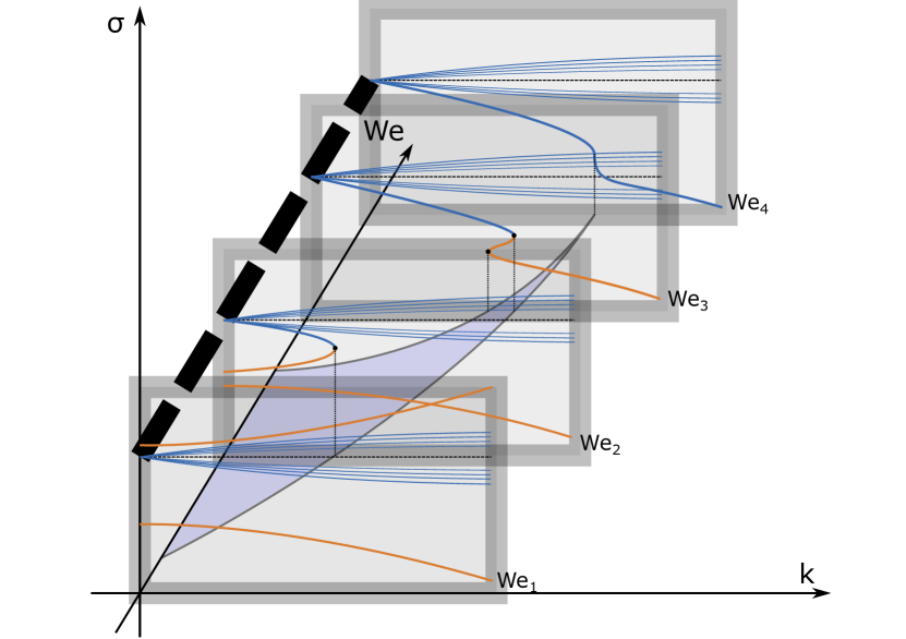
Figure 6: A schematic showing the loci of the pairs of folding points, associated with the hysteretic dispersion curves, which leads to the inviscidly stable island in the $We-k$ plane.

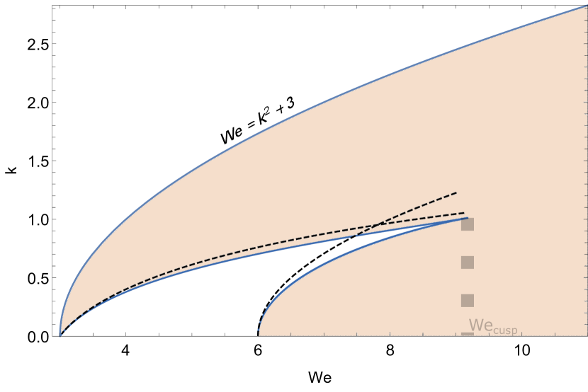
(a) $n=2$

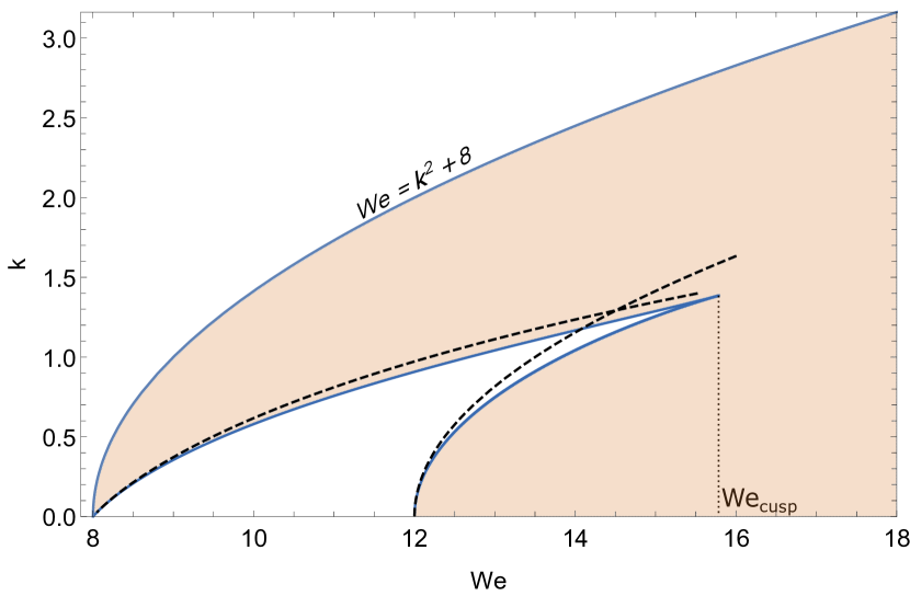
(b) $n=3$

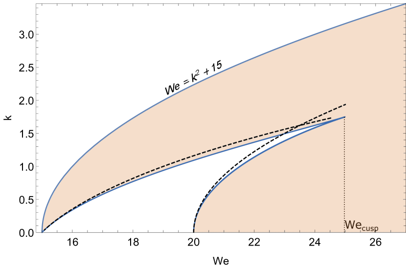
(c) $n=4$

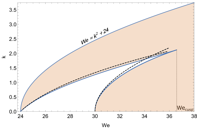
(d) $n=5$

Figure 7: Depiction of the stable islands in the $We-k$ plane for $n=2,3,4$ and $5$. Blue curves denote both, the outer boundary ($We=n^{2}+k^{2}-1$) and the numerically obtained boundaries of the inviscidly stable island within; the shaded region between these boundaries denotes the inviscidly unstable region. The dashed black curves denote the small-$k$ asymptotes for the island boundaries; the lower branch asymptote is $k\thicksim\sqrt{\frac{n^{2}-1}{n(n+1)}(We-n(n+1))}$ and that for the upper branch is obtained by simultaneously solving $d\sigma/dk=\infty$ with eq. 7 for small $k$.

The general behavior of the dispersion curves with increasing $We$, highlighted above, holds for all $n$’s greater than unity. Fig. 5 shows an analogous behavior of the eigenspectrum for $n=4$ with $We_{\text{cusp}}\approx 25$. The dispersion curves, such as those in Figs. 4 and 5, may be stacked upon one another, along the $We$-axis, so as to demarcate the regions of inviscid stability in the $We-k$ plane for each $n$. Fig. 6 shows schematically how this may be achieved (the unstable wavenumber ranges have been omitted for clarity). With varying $We$, projections of the pair of folding points associated with each hysteretic dispersion curve (the black dots in Figs. 4(c), 5(c) and 6), that mark the intermediate stable interval in the $\sigma-k$ plane, yield the two branches of a stable island in the $We-k$ plane. The picture is that of a cusp catastrophe (Zeeman (1976)), implying that the aforementioned pair of branches terminates in a cusp. The points of coalescence between a capillary mode and the lowest retrograde Coriolis mode (Fig. 4(b) and 5(b)) yield the upper branch of the stable island, while those between the two capillary modes (Fig. 4(c) and 5(c)) yield the lower branch. The cusp-shaped islands of inviscid stability in the $We-k$ plane, for $n=2,3,4$ and $5$, are shown in Fig. 7. While closed form expressions for the boundaries of these islands are not available, one may nevertheless obtain their small-$k$ approximations. For the lower branch, one has $\sigma\rightarrow n-1$ for $k\to 0$; the resulting limiting form of the dispersion relation gives the required approximation as $k\thicksim\sqrt{\frac{n^{2}-1}{n(n+1)}(We-n(n+1))}$. For the upper branch, however, $(\sigma-n)/k$ remains $\mathcal{O}(1)$ as $k\to 0$. Since this remains true for all of the Coriolis mode branches, the upper branch asymptote is obtained by exploiting the fact that the slope of the hysteretic dispersion curve diverges at the turning points. Thus, simultaneously solving eq. 7 with $d\sigma/dk\to\infty$ for $k\rightarrow 0$ yields the small-$k$ approximation for the upper branch. These approximations have been shown as dashed black curves in Fig. 7, where they are seen to compare well to the numerically determined island boundaries well beyond the rigorous interval of validity $(k\ll 1)$. While one expects the $We-k$ plane to remain similar in form for $n>5$, the scenario for $n=1$ is essentially different, and is analyzed in the Appendix. In this case, there exists only one stable island that extends to infinity along the $We$ axis. The exceptional behavior is not entirely unexpected, given that the limit $k\to 0$ is a singular one - $n=1$ corresponds to a mere translation of the rotating column in the planar limit.

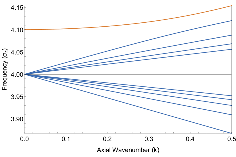
(a) $We=14.25$

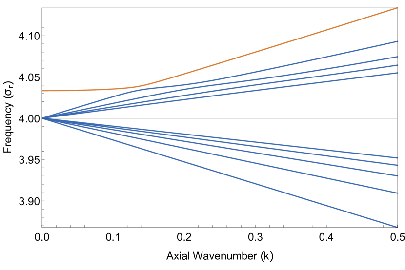
(b) $We=14.75$

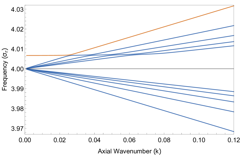
(c) $We=14.95$

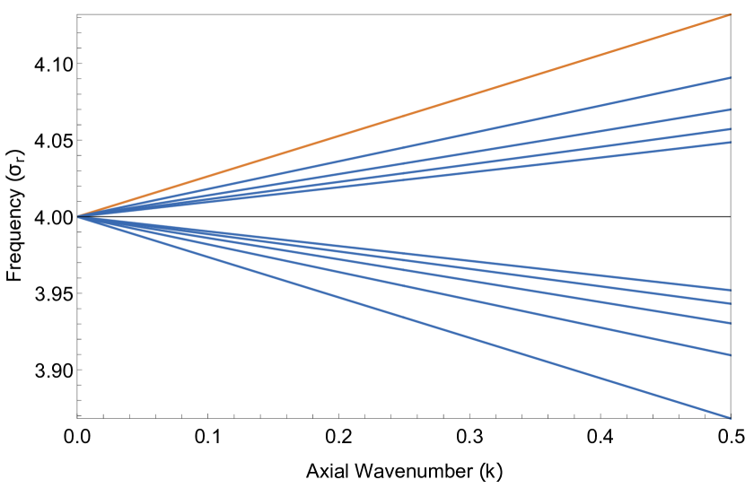
(d) $We=15$

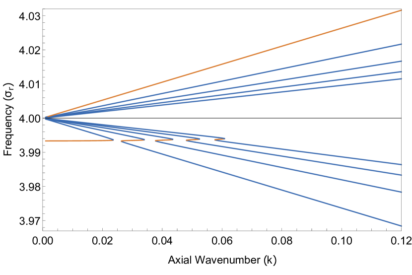
(e) $We=15.05$

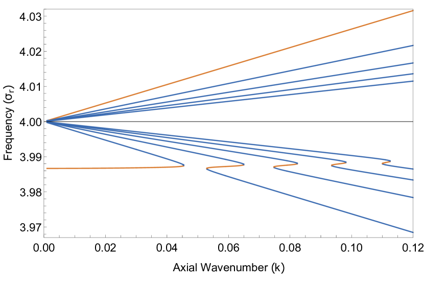
(f) $We=15.1$

Figure 8: Dispersion curves ($\sigma$ vs $k$) for $n=4$ and $We$ close to $n^{2}-1$. At $We=n^{2}-1$ the capillary mode splits into two and yields a new retrograde mode (also shown in orange) which subsequently undergoes an infinite sequence of coalescences with the retrograde Coriolis modes for higher $We$.

The discussion along with the preceding figures establish the following behavior. With increasing $We$, the upper capillary branch moves down to lower frequencies, appearing to cross the zero-Doppler-frequency line $\sigma=n$ in the process, and thereafter, undergoes a pair of coalescences (one with the lowest Coriolis mode, and the other with the lower capillary branch). These coalescences lead to intermediate unstable ranges of wavenumbers which, with varying $We$, trace out a stable island in the $We-k$ plane (see Fig. 7). There are two subtle aspects with regard to this general behavior that need amplification, however. The first is that the upper capillary branch does not, in fact, end up crossing $\sigma=n$ (hence, the usage ’appears to’ in all the instances above). Instead, as shown in Fig. 8, at $We=n^{2}-1$, when the zero-$k$ frequency of this branch equals $\sigma=n$ (Fig. 8(d)), the capillary branch stops moving downward as a whole; instead, a new discrete mode emanates from $\sigma=n$, and continues down into the retrograde frequency range with further increase in $We$ (Figs. 8(e) and 8(f)). Further, even as the upper capillary branch descends towards $\sigma=n$, for $We$ just below $n^{2}-1$, it never crosses the lower cograde Coriolis branches. These ‘avoided crossings’ are illustrated via suitably magnified views in Figs. 8(a)-8(c), and arise from the Krein signature criterion, required for unstable coalescences between different modal branches, not being satisfied for cograde modes [Mackay & Meiss (1987); Chernyavsky et al. (2018); Fukumoto (2003)].

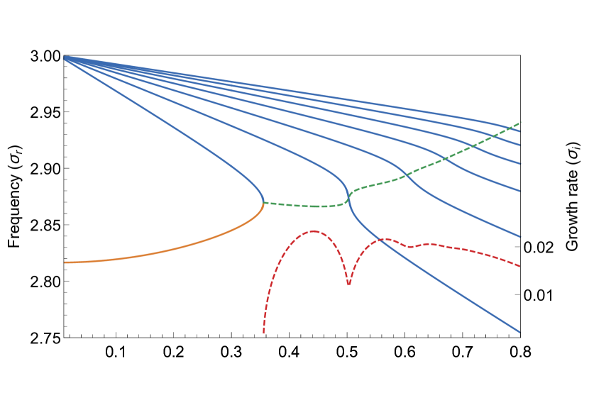
(a) $We=9$: A single coalescence between a capillary and a Coriolis mode.

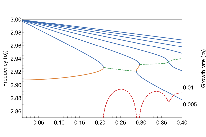
(b) $We=8.5$: The capillary-Coriolis coalescence plus a single hysteretic dispersion curve.

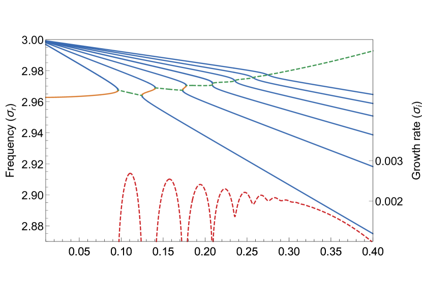
(c) $We=8.2$: The capillary-Coriolis coalescence plus three hysteretic dispersion curves.

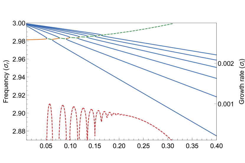
(d) $We=8.1$. The capillary-Coriolis coalescence plus four hysteretic dispersion curves.

Figure 9: An increasing number of retrograte dispersion curves exhibit a hysteretic character for $We\to(n^{2}-1)^{+}$; the figures show this behavior for $n=3$.

The second subtle aspect is related to the retrograde mode above that bifurcates from the cograde capillary mode at $\sigma=n$. In moving further down towards $\sigma=n-1$ with increasing $We$ (at which point this mode undergoes a coalescence with the lower capillary branch, leading to an unstable wavenumber interval $(0,k_{2})$, as illustrated in Figs. 4(c) and 5(c)), the mode must end up crossing an infinite number of Coriolis mode branches, in turn implying the possibility of an infinite hierarchy of coalescences, instead of just the single one with the lowermost (retrograde) Coriolis branch shown in Figs. 4(b) and 5(b). Note that the infinite number of crossings must occur in the neighborhood of $\sigma=n$ which, from eq. 4, corresponds to $We=n^{2}-1$. Therefore, one may verify the existence of such a hierarchy of crossings by checking for the occurrence of coalescences in the eigenspectra in the vicinity of $We=n^{2}-1$. It turns out that all of the crossings of the aforementioned retrograde mode with the retrograde Coriolis modes lead to coalescences, and thence, hysteretic dispersion curves with intermediate unstable $k$-intervals. The number of such hysteretic curves increases rapidly as $We$ approaches $n^{2}-1$ from above. Fig. 9 depicts the increasing number of hysteretic dispersion curves that result for $n=3$ for $We\rightarrow 8^{+}$; there is one coalescence for $We=8.5$, three for $We=8.2$ and four for $We=8.1$, besides the original coalescence between the new retrograde mode and the lowest Coriolis mode, with successive coalescences occurring at progressively smaller $k$. Fig. 10 provides a magnified view of the ensemble of dispersion curves for $We=8.1$, emphasizing the rapid oscillations in the growth rate owing to the multiple closely-spaced intervals of stability. Similar to Fig. 7, each of these hysteretic intervals marks out a stable island in the $We-k$ plane. Therefore, in the inviscid limit, there appears to be an infinite hierarchy of neutrally stable islands (each of these associated with a cusp catastrophe, or a fold in the three-dimensional surface characterizing the $We-k-\sigma$ relationship as illustrated in Fig. 6) enclosed within the viscously unstable region given by $We>n^{2}+k^{2}-1$. This infinite hierarchy of inviscidly stable islands only appears above, and not below, the viscous threshold since, as already pointed out, the cograde modes exhibit avoided collisions (Figs.8(a)-8(c)), while the retrograde modes coalesce, yielding complex eigenvalues, consistent with their respective Krein signatures. The higher-order stable islands are much smaller than the leading one, and decrease in size rapidly, eventually asymptoting to the limit point $(We,k)=(n^{2}-1,0)$. The resulting picture in the $We-k$ plane is illustrated in Fig. 11 for $n=2,3,4$ and $5$. Each of the sub-figures shows five leading satellite islands besides the main island, of what is likely an infinite hierarchy. As implied by Fig. 10, a consequence of this infinite hierarchy is a rapid alternation of regions of stability and instability as one increases $k$ for a fixed $We$, and thence, a rapidly fluctuating growth rate with changing $k$.

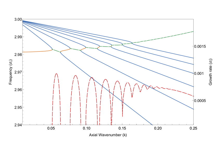
Figure 10: A magnified view of Fig. 9(d); $We=8.1;n=3$. Note the multiple hysteretic dispersion curves (four, besides the original) and corresponding oscillations in the growth rate.

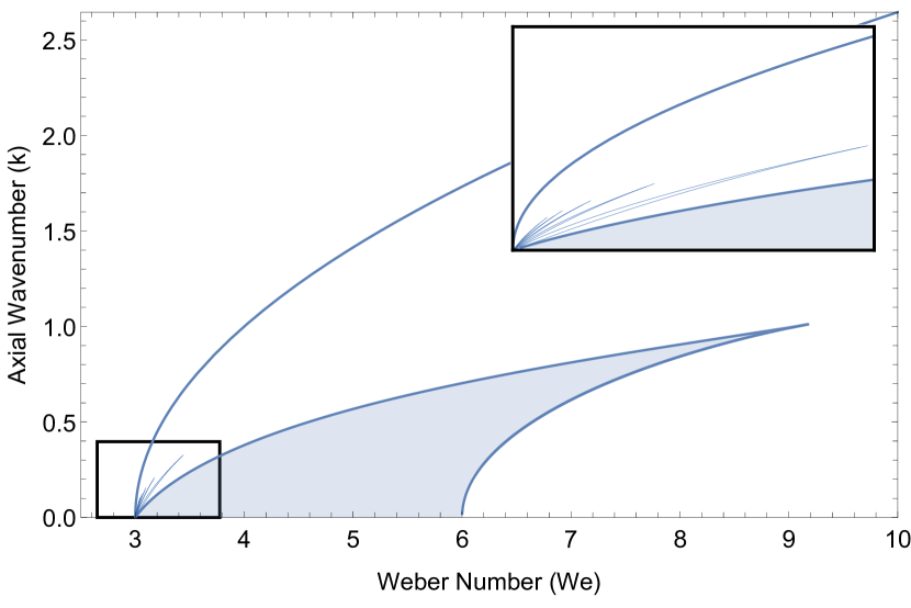
(a) n = 2

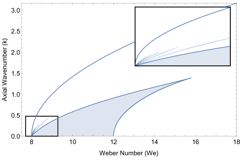
(b) n = 3

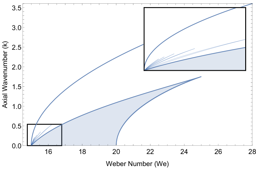
(c) n = 4

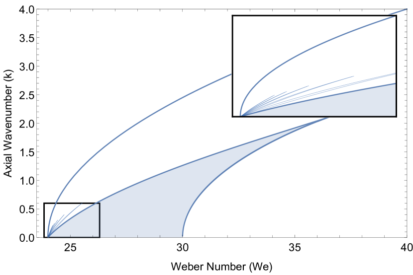
(d) n = 5

Figure 11: The main and satellite islands of inviscid stability, in the $We-k$ plane, for $n=2,3,4$ and $5$. Magnified views, of five of the infinite hierarchy of satellite islands, appear in the insets.

3 Conclusion

In this paper, we have analyzed the inviscid stability of a rotating liquid column as a function of $We$, and the axial and azimuthal wavenumbers ($k$ and $n$) of the imposed perturbation, with a focus on the entire eigenspectrum that includes a pair of capillary modes and an infinite hierarchy of Coriolis modes in the general case. While it is known that a viscous rotating column becomes unstable if and only if $We>k^{2}+n^{2}-1$, consideration of the full eigenspectrum highlights the intricate nature of the inviscidly unstable region in the $We-k$ plane. The intricacy arises from the likelihood of an infinite hierarchy of coalescences between pairs of dispersion curves in the neighborhood of the planar viscous threshold $(We=n^{2}-1)$. As illustrated in Fig. 11, these coalescences appear to lead to an infinite hierarchy of inviscidly stable islands within the viscously unstable region $(We>n^{2}+k^{2}-1)$ in the $We-k$ plane; each of these islands corresponds to a fold in the $We-k-\sigma$ surface in three dimensions (see Fig. 6). The existence of these islands explains why $We<n^{2}+k^{2}-1$ only serves as a sufficient condition for stability in the inviscid limit [Pedley (1967)]; evidently, one can be stable even when $We>n^{2}+k^{2}-1$, provided one is inside any of these islands. Thus, the necessary and sufficient condition for inviscid instability would require $We>n^{2}+k^{2}-1$, and in addition, that the $(We,k,n)$ triplet chosen lies outside the inviscid islands identified in Fig. 11. It is not possible to provide a precise expression for this criterion since, as already pointed out, closed form expressions for the island boundaries are not known; although, the small-$k$ asymptotes appear to serve as useful approximations especially for the larger $n$’s (see Fig. 7). Interestingly, it has been shown in the Appendix of Weidman et al. (1997) that one may again obtain only a sufficient condition for inviscid stability for the analogous two-fluid system. Thus, for a configuration consisting of a central column of a denser liquid and an annular domain of a lighter one, both being in a state of rigid-body rotation, the sufficient condition for inviscid stability becomes

$$\mathit{We}_{1}-\mathit{We}_{2}<k^{2}+n^{2}-1$$ (8)

where $\mathit{We}_{1}$ is the Weber number defined using the density of the inner fluid and $\mathit{We}_{2}$ is that defined using the density of the outer fluid. Although the viscous problem, and therefore, the viscous stability criterion for the two-fluid system problem has not yet been examined, the discussion presented here suggests an analogous relationship between the viscous and inviscid criteria.

The discovery of an infinite hierarchy of inviscidly stable islands in the $We-k$ plane also has implications for viscous stability for large but finite $Re$. As shown in Fig. 10, for the case $n=3$ and $We=8.1$, the inviscid growth rate oscillates rapidly between zero and order-unity values, with the oscillations becoming increasingly dense and rapid for $We\rightarrow 8^{+}$ (the value of $n^{2}-1$ for $n=3$); interestingly, although the growth rates decrease for $We\rightarrow(n^{2}-1)^{+}$, as expected, the amplitude of the oscillations, for a fixed $We$, does not appear to decay with increasing order of the modal coalescence, the order here referring to the modal index of the (retrograde) Coriolis mode involved in the particular coalescence. Now, for large but finite $Re$, one expects only a finite number of oscillations regardless of the proximity of $We$ to $n^{2}-1$. This is because, as mentioned in section 2.2, the viscous decay rates for planar perturbations can attain arbitrarily high values for large enough modal indices, owing to the vanishingly small radial scale associated with the eigenfunction. Thus, for finite $Re$ however large, one expects the (inviscid) growth rate associated with modal coalescences above a certain threshold order to be overwhelmed by viscous decay. Nevertheless, for an $Re$ large enough that the spacings between adjacent islands is greater than $O(Re^{-2})$, one expects rapid oscillations in the growth rate between order-unity values between the islands, and $O(Re^{-1})$ values within them. While the $Re$’s required to see substantial growth-rate oscillations requires a full viscous calculation, it does appear that the $Re$’s involved might be very large. In contrast, experiments on the rotating liquid column have only accessed a maximum $Re$ of $O(10)$; see Kubitschek & Weidman (2008).

The question of $Re$ being large enough for one to be able to observe the aforementioned oscillations in the (viscous) growth rate leads us to the astrophysical analog of the configuration examined thus far - that of a rotating self-gravitating fluid column, which may be likened to a large-scale filamentary structure; such structures appear to have a ubiquitous presence in the interstellar medium [André (2017)]. Chandrasekhar and Fermi performed one of the earliest studies on the stability of a self-gravitating column [see Chandrasekhar & Fermi (1953); Chandrasekhar & Lebovitz (1964)]. Their calculations were done in the incompressible limit and revealed an axisymmetric instability. Analogous to the Rayleigh-Plateau instability of the liquid column, the axisymmetrically deformed fluid column has a lower gravitational potential energy than the original columnar configuration for sufficiently long-wavelength perturbations and is therefore unstable to all axisymmetric perturbations with $k<1.0668$. Subsequently, Ostriker extended Chandrasekhar and Fermi’s analysis to a compressible base state, evaluating the base-state density profiles for different values of the polytropic index [Ostriker (1964a)]. Compressibility leads to an inhomogeneous base state of a finite radius, the isothermal case being an exception in leading to an infinite radius. Thus, Ostriker (1964b) analyzed the effects of compressible perturbations on a base state that is a solution of the incompressible equations (a homogeneous finite-radius cylinder). Later, Nagasawa (1987) carried out a stability calculation for the inhomogeneous density profile corresponding to the aforementioned isothermal base state, and concluded that the isothermal problem is only unstable to axisymmetric disturbances, similar to Chandrasekhar and Fermi’s analysis above. The critical wavelength obtained by Nagasawa (1987) was also found earlier by Stodólkiewicz (1963), who had carried out a restricted stability analysis of the isothermal base state only to axisymmetric disturbances. Due to their prominent role in star formation, studies on the gravitational instability of filamentary molecular clouds continue to garner attention [McKee & Ostriker (2007)]. Recently Motiei et al. (2021) have revisited the problem of axisymmetric stability of self-gravitating fluid cylinders, including effects of an external pressure, an axial magnetic field and a wide array of non-isothermal equations of state that are a better representation of observations.

Rotation is ubiquitous in self-gravitating filaments, and Hansen et al. (1976) were one of the first to examine the equilibrium and stability of an isothermal and uniformly rotating cylinder. The inclusion of rotation introduced an unusual feature to the equilibrium state - a (spatially) damped oscillatory density profile. Hansen et al. (1976) analyzed the stability of the rotating base states of a finite radius to two-dimensional disturbances. They found that rotation renders cylinders, exceeding a critical size, unstable to non-axisymmetric disturbances. Freundlich et al. (2014) have recently studied the stability of a polytropic rotating cylinder using a local stability analysis. Sadhukhan et al. (2016) have extended the local stability analysis to polytropic rotating cylinders, with the addition of a magnetic field, and observe that the background rotation acts to reduce the unstable growth rates. Thus, there exist instances in the literature of rotation having conflicting roles - in terms of both stabilizing and destabilizing self-gravitating masses. To comprehensively understand the role that rotation plays in the stability of filamentary molecular clouds, there is an imminent need for a global three-dimensional stability analysis of rotating polytropic cylinders. In this section, however, we only look at the limiting case of an incompressible cylinder - the rotating version of Chandrasekhar and Fermi’s seminal study. This is because our focus here is to primarily draw an analogy between the cohesive forces of surface tension and gravitation; we show below that a rotating self-gravitating incompressible fluid column exhibits an infinite hierarchy of cusp-catastrophes analogous to the rotating liquid column above. Although beyond the scope of the present calculation, we expect our findings to continue to be relevant for compressible self-gravitating columns.

A linear stability analysis of a self-gravitating cylinder, in a state of rigid-body rotation, readily furnishes the following dispersion relation:

$$\alpha\frac{J_{n-1}(\alpha)}{J_{n}(\alpha)}-\frac{\frac{\Omega^{2}}{2\pi\rho G}(4-(\sigma-n)^{2})}{\frac{\Omega^{2}}{2\pi\rho G}-(1-2K_{n}(k)I_{n}(k))}-n\left(1+\frac{2}{(\sigma-n)}\right)=0,$$ (9)

where $\frac{\Omega^{2}}{2\pi\rho G}$ is the analog of the Weber number for the self-gravitating case, in measuring the relative importance of gravitational and centrifugal forces, $G$ being the gravitational constant. Let us now define

$$\mathit{We_{G}}=f(n,k)\,\frac{\Omega^{2}}{2\pi\rho G},$$ (10)

where $f(n,k)=\frac{k^{2}+n^{2}-1}{1-2I_{n}(k)K_{n}(k)}$, so that we have, in terms of $\mathit{We_{G}}$, a dispersion relation identical to that in eq. 7. Since $f(n,k)$ is a monotonically increasing function of $k$ for a given $n$, one has a unique value of $\frac{\Omega^{2}}{2\pi\rho G}$ for every $\mathit{We_{G}}$. The $\frac{\Omega^{2}}{2\pi\rho G}-k$ plane will then be topologically equivalent to the $\mathit{We_{G}}-k$ plane, and thence, to the $\mathit{We}-k$ plane of the rotating liquid column seen earlier. The resulting infinite hierarchy of cusp-catastrophes for the rotating self-gravitating fluid column, and its comparison with the hierarchy already seen above, for the rotating liquid column (with surface tension), is shown in Fig. 12.

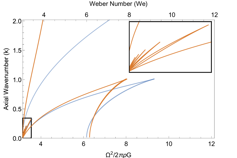
(a) n = 2

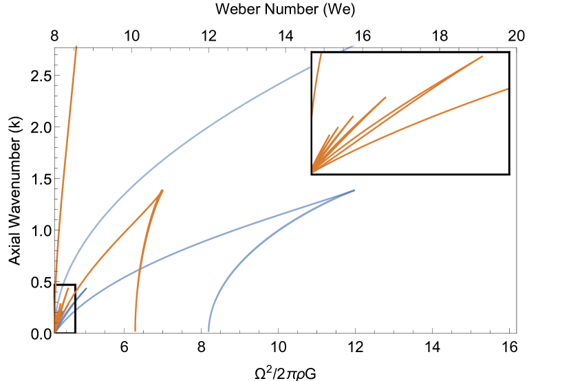
(b) n = 3

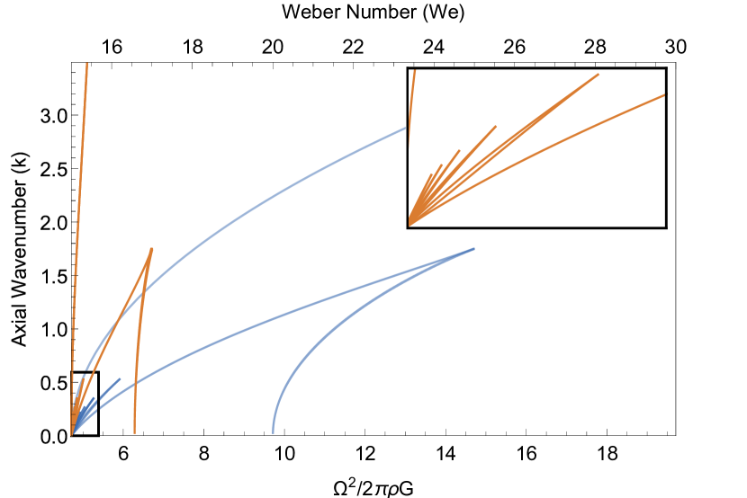
(c) n = 4

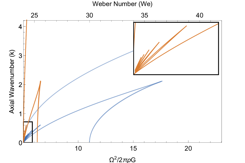
(d) n = 5

Figure 12: Comparison of the inviscidly stable islands for the surface-tension (blue) and self-gravitating (orange) cases for $n=2,3,4$ and $5$. The insets in each figure show magnified views of the first five satellite islands for the self-gravitating column.

Appendix A Stability criteria for $n=1$

For planar perturbations with $n=1$, one sees from eq. 4 that $\sigma$ vanishes identically for all non-zero $We$. Therefore, the inviscid threshold, $We=n(n+1)$, is of no relevance in this case, and there can be no analog of the different $We$-regimes that exist for $n\geq 2$ (see Figs. 4(a)-4(d)). As already stated in the main text, this is expected since a planar perturbation for $n=1$ corresponds to a mere translational displacement. Further, for $n\geq 2$, the pair of planar frequencies, corresponding to the two capillary branches, are widely separated, and symmetrically distributed about $\sigma=n-1$, for small $We$. The motion of the upper capillary branch down towards $\sigma=n$, with increasing $We$, and the subsequent birthing of a new retrograde mode at $\sigma=n$, is essential for the infinite hierarchy of coalescences in the $\sigma-k$ plane, and thence, for the infinite hierarchy of inviscidly stable islands in the $We-k$ plane. In contrast, for $n=1$, $\sigma=0$ is a double root of the governing quadratic. Thus, a second mode emanates from $\sigma=0$, with increasing $k$, in addition to the retrograde capillary mode, and may be likened to the retrograde mode above, for $n\geq 2$, that undergoes coalescences with the Coriolis modes. But, for $n=1$, this mode is already below the infinite hierarchy of retrograde Coriolis modes even at the smallest $We$ (see Fig. 13(a) below) , and one may only expect a merger with the lowest member of the Coriolis hierarchy. As a result, one expects a leading stable island, but no satellite islands, in the $We-k$ plane.

In fact, the nature of the dispersion curves for $n=1$ does not change qualitatively with increasing $We$. One observes a single coalescence, and thence, a single unstable interval bounded away from $k=0$, for any finite $We$. Figs. 13(a)-13(d) confirm this behavior for $We$ ranging from 1 to 10. As $We=10$ is significantly greater than the hypothetical threshold ($n(n+1)=2$), we do not expect this picture to alter for greater $We$’s and the resulting stable island in the $We-k$ plane would thus extend to infinity (Fig. 13(e)). This, once again, points to the absence of distinct $We$ regimes observed for $n\geq 2$. The growth rate and range of unstable wavenumbers shown in 13(d) are consistent with Fig. 4 of Weidman et al. (1997). Finally, from the growth rate perspective, the $n=1$ mode remains subdominant for all $Re$ greater than $1.166$ (approx). As shown by Kubitschek & Weidman (2007a) the azimuthal wavenumber of the dominant perturbation jumps from $n=0$ to $n=2$ beyond $Re\approx 1.166$, and then to higher $n$’s with increasing $We$. Thus, the anomalous behavior of $n=1$ is less important in the limit of large $Re$ as, for instance, in the astrophysical context above.

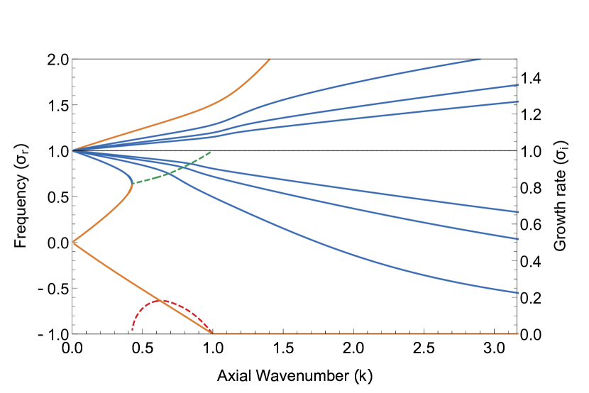
(a) $We=1$

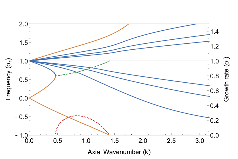
(b) $We=2$

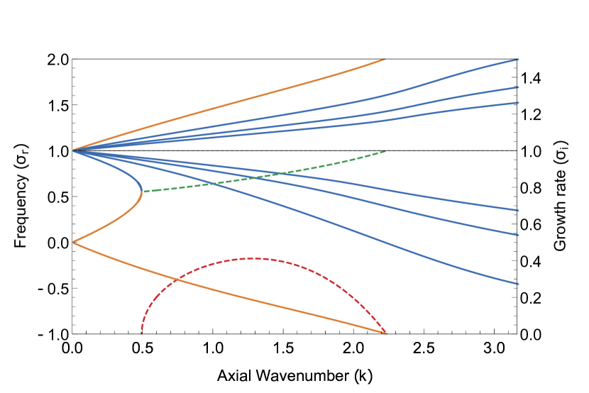
(c) $We=5$

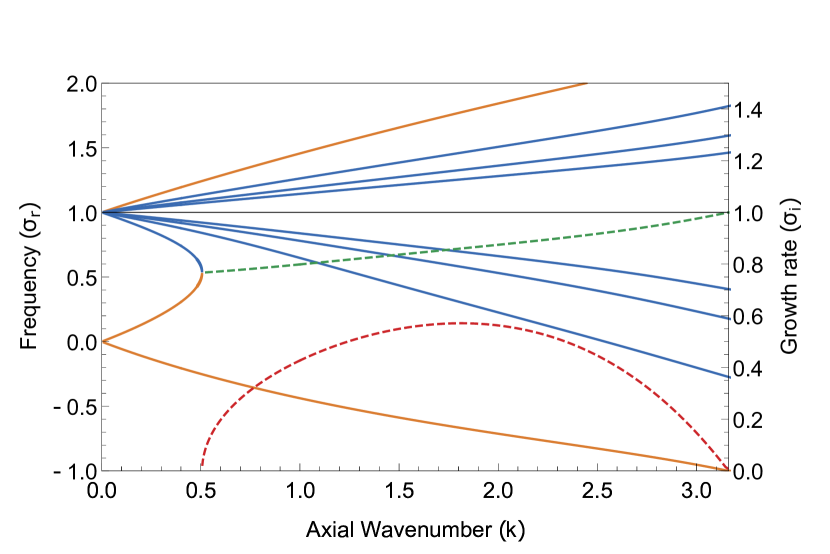
(d) $We=10$

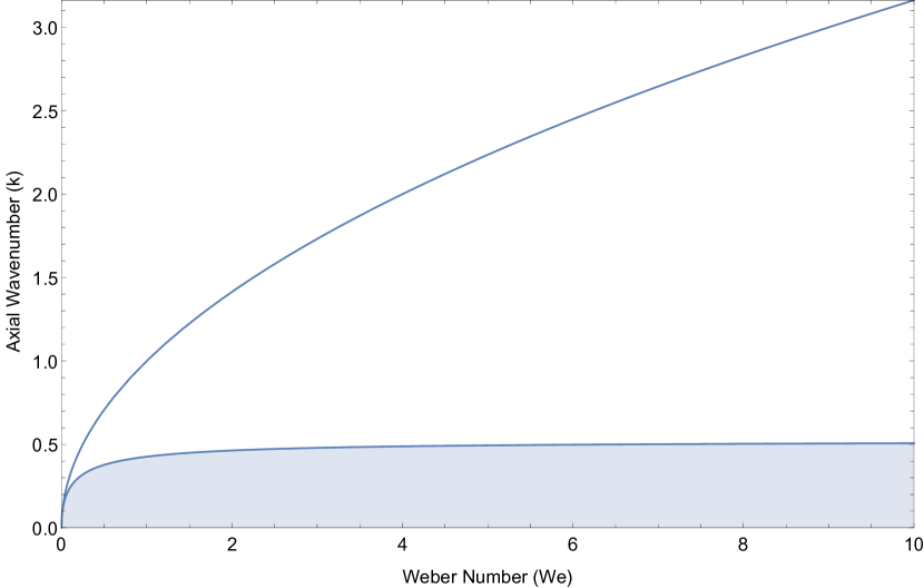
(e) Region of stability for n=1

Figure 13: Dispersion curves for $n=1$ (Figs. (a-d)); the solid blue curves indicate the Coriolis modes, the solid orange curves indicate the capillary modes and the dashed curves indicate real (red) and imaginary (green) parts of the unstable modes. Fig. (e) depicts the stable island generated as a result of coalescence of the lowest Coriolis mode and the retrograde capillary mode.

References

- André (2017) André, Philippe 2017 Interstellar filaments and star formation. Comptes Rendus Geoscience 349 (5), 187–197.
- Benjamin (1959) Benjamin, T Brooke 1959 Shearing flow over a wavy boundary. Journal of Fluid Mechanics 6 (2), 161–205.
- Chandrasekhar (1981) Chandrasekhar, S. 1981 The Gravitational Instability of an Infinite Cylinder, pp. 516–523. Dover Books on Physics Series 1. Dover Publications.
- Chandrasekhar & Fermi (1953) Chandrasekhar, Subrahmanyan & Fermi, Enrico 1953 Problems of gravitational stability in the presence of a magnetic field. The Astrophysical Journal 118, 116.
- Chandrasekhar & Lebovitz (1964) Chandrasekhar, S & Lebovitz, Norman R 1964 Non-radial oscillations of gaseous masses. The Astrophysical Journal 140, 1517.
- Chernyavsky et al. (2018) Chernyavsky, A., Kevrekidis, P. G. & Pelinovsky, D. E. 2018 Krein Signature in Hamiltonian and -Symmetric Systems. Springer Tracts Mod. Phys. 280, 465–491.
- Freundlich et al. (2014) Freundlich, Jonathan, Jog, Chanda J & Combes, Françoise 2014 Local stability of a gravitating filament: a dispersion relation. Astronomy & Astrophysics 564, A7.
- Fukumoto (2003) Fukumoto, Yasuhide 2003 The three-dimensional instability of a strained vortex tube revisited. Journal of Fluid Mechanics 493, 287.
- Gillis (1961) Gillis, J 1961 Stability of a column of rotating viscous liquid. In Mathematical Proceedings of the Cambridge Philosophical Society, , vol. 57, pp. 152–159. Cambridge University Press.
- Gillis & Kaufman (1962) Gillis, J & Kaufman, B 1962 The stability of a rotating viscous jet. Quarterly of Applied Mathematics 19 (4), 301–308.
- Hansen et al. (1976) Hansen, Carl J, Aizenman, Morris L & Ross, Randy L 1976 The equilibrium and stability of uniformly rotating, isothermal gas cylinders. The Astrophysical Journal 207, 736–744.
- Henderson & Barenghi (2002) Henderson, KL & Barenghi, CF 2002 The stability of a superfluid rotating jet. Journal of Physics A: Mathematical and General 35 (45), 9645.
- Hocking (1960) Hocking, L. M. 1960 The stability of a rigidly rotating column of liquid. Mathematika 7 (1), 1–9.
- Hocking & Michael (1959) Hocking, L. M. & Michael, D. H. 1959 The stability of a column of rotating liquid. Mathematika 6 (1), 25–32.
- Kubitschek & Weidman (2007a) Kubitschek, JP & Weidman, PD 2007a The effect of viscosity on the stability of a uniformly rotating liquid column in zero gravity. Journal of Fluid Mechanics 572, 261.
- Kubitschek & Weidman (2007b) Kubitschek, JP & Weidman, PD 2007b Helical instability of a rotating viscous liquid jet. Physics of Fluids 19 (11), 114108.
- Kubitschek & Weidman (2008) Kubitschek, JP & Weidman, PD 2008 Helical instability of a rotating liquid jet. Physics of Fluids 20 (9), 091104.
- Mackay & Meiss (1987) Mackay, R S & Meiss, J D 1987 Stability of Equilibria of Hamiltonian Systems, pp. 137–153. CRC Press.
- McKee & Ostriker (2007) McKee, Christopher F & Ostriker, Eve C 2007 Theory of star formation. Annu. Rev. Astron. Astrophys. 45, 565–687.
- Miles (1957) Miles, John W 1957 On the generation of surface waves by shear flows. Journal of Fluid Mechanics 3 (2), 185–204.
- Motiei et al. (2021) Motiei, Mohammad Mahdi, Hosseinirad, Mohammad & Abbassi, Shahram 2021 Gravitational instability of non-isothermal filamentary molecular clouds in presence of external pressure. Monthly Notices of the Royal Astronomical Society 502 (4), 6188–6200.
- Nagasawa (1987) Nagasawa, Mikio 1987 Gravitational instability of the isothermal gas cylinder with an axial magnetic field. Progress of Theoretical Physics 77 (3), 635–652.
- Ostriker (1964a) Ostriker, J 1964a The equilibrium of polytropic and isothermal cylinders. The Astrophysical Journal 140, 1056.
- Ostriker (1964b) Ostriker, J 1964b On the oscillations and the stability of a homogeneous compressible cylinder. The Astrophysical Journal 140, 1529.
- Pedley (1967) Pedley, TJ 1967 The stability of rotating flows with a cylindrical free surface. Journal of Fluid Mechanics 30 (1), 127–147.
- Plateau (1873) Plateau, Joseph Antoine Ferdinand 1873 Statique expérimentale et théorique des liquides soumis aux seules forces moléculaires. Gauthier-Villars.
- Rayleigh (1878) Rayleigh, Lord 1878 On the instability of jets. Proceedings of the London mathematical society 1 (1), 4–13.
- Rosenthal (1962) Rosenthal, DK 1962 The shape and stability of a bubble at the axis of a rotating liquid. Journal of Fluid Mechanics 12 (3), 358–366.
- Roy et al. (2021) Roy, Anubhab, Garg, Piyush, Reddy, Jhumpal Shashikiran & Subramanian, Ganesh 2021 Inertio-elastic instability of a vortex column, arXiv: 2101.00805.
- Roy & Subramanian (2014) Roy, Anubhab & Subramanian, Ganesh 2014 Linearized oscillations of a vortex column: the singular eigenfunctions. Journal of Fluid Mechanics 741, 404–460.
- Sadhukhan et al. (2016) Sadhukhan, Shubhadeep, Mondal, Surajit & Chakraborty, Sagar 2016 Stability of rotating self-gravitating filaments: effects of magnetic field. Monthly Notices of the Royal Astronomical Society 459 (3), 3059–3067.
- Stodólkiewicz (1963) Stodólkiewicz, JS 1963 On the gravitational instability of some magneto-hydrodynamical systems of astrophysical interest. part iii. Acta Astronomica 13, 30–54.
- Weidman (1994) Weidman, Patrick 1994 Stability criteria for two immiscible fluids rigidly rotating in zero gravity. Revue Roumaine des Sciences Techniques. Série de Mécanique Appliquée 39.
- Weidman et al. (1997) Weidman, PD, Goto, M & Fridberg, A 1997 On the instability of inviscid, rigidly rotating immiscible fluids in zero gravity. Zeitschrift für angewandte Mathematik und Physik ZAMP 48 (6), 921–950.
- Zeeman (1976) Zeeman, E Christopher 1976 Catastrophe theory. Scientific American 234 (4), 65–83.