MCMC-based Voigt Profile fitting to a Mini-BAL System in the Quasar UM675

Abstract

We introduce a Bayesian approach coupled with a Markov Chain Monte Carlo (MCMC) method and the maximum likelihood statistic for fitting the profiles of narrow absorption lines (NALs) in quasar spectra. This method also incorporates overlap between different absorbers. We illustrate and test this method by fitting models to a “mini-broad” (mini-BAL) and six NAL profiles in four spectra of the quasar UM675 taken over a rest-frame interval of 4.24 years. Our fitting results are consistent with past results for the mini-BAL system in this quasar by Hamann et al. (1997b). We also measure covering factors ($C_{\rm f}$) for two narrow components in the C IV and N V mini-BALs and their overlap covering factor with the broad component. We find that $C_{\rm f}$ (N V) is always larger than $C_{\rm f}$ (C IV) for the broad component, while the opposite is true for the narrow components in the mini-BAL system. This could be explained if the broad and narrow components originated in gas at different radial distances, but it seems more likely to be due to them produced by gas at the same distance but with different gas densities (i.e., ionization states). The variability detected only in the broad absorption component in the mini-BAL system is probably due to gas motion since both $C_{\rm f}$ (C IV) and $C_{\rm f}$ (N V) vary. We determine for the first time that multiple absorbing clouds (i.e., a broad and two narrow components) overlap along our line of sight. We conclude that the new method improves fitting results considerably compared to previous methods.



1. Introduction

Astronomical objects along our line of sight to distant quasars will produce absorption lines in the spectra of those quasars (hereafter, quasar absorption lines or QALs). The absorbers include not only cosmologically intervening objects, like foreground galaxies and intergalactic medium (IGM) (hereafter, intervening QALs), but also gas clouds that are physically associated with the quasars themselves such as AGN outflows (hereafter, intrinsic QALs). These absorption lines have historically been studied by counting their numbers as a function of redshift ($dN/dz$) for various transitions to place constraints on their physical sizes and comoving number densities (e.g., Steidel 1990; Bechtold 1994; Lanzetta et al. 1995). With the advent of 8–10 m class telescopes and their high-dispersion spectrographs such as the Keck telescope with the High Resolution Echelle Spectrometer (HIRES), the Very Large Telescope (VLT) with the Ultraviolet and Visual Echelle Spectrograph (UVES), and the Subaru telescope with the High Dispersion Spectrograph (HDS), we are now able to measure physical parameters in addition to the absorption redshift ($z_{\rm abs}$), e.g., the column density ($N$), and the Doppler parameter ($b$) by fitting Voigt profiles (VPs) to the absorption lines.

The intrinsic QALs are generally blueshifted from the quasar emission redshift by up to $\sim$0.2–0.3 c (Hamann et al., 2018), which suggests that they are accelerated away from the quasar by several possible mechanisms, including radiative pressure (Murray et al., 1995; Proga et al., 2000), magnetocentrifugal force (e.g., Everett, 2005), and thermal pressure (e.g., Chelouche & Netzer, 2005). They are usually classified into three categories according to their line widths: broad absorption lines (BALs) with total FWHM $\geq$ 2,000 km/s, narrow absorption lines (NALs) with FWHM $\leq$ 500 km/s, and an intermediate subclass (mini-BALs). The difference in line width is often explained by the inclination angle of our line of sight relative to the direction of motion of the wind (e.g., Elvis, 2000; Ganguly et al., 2001; Itoh et al., 2020) or the stage of quasar evolution (e.g., Farrah et al., 2007), although it may also depend on the emission line outflow properties and/or the hardness of the ionizing spectral energy distribution (e.g., Rankine et al. 2020). Intrinsic QALs may play an important role in providing energy and momentum feedback to the interstellar medium (ISM) and circumgalactic medium (CGM) of their host galaxies and the surrounding IGM, and may play a role in regulating star formation activity in their host galaxies (e.g., Springel et al., 2005).

In past studies of QALs, several $\chi^{2}$-based VP fitting codes have been used, including VPFIT (Carswell et al., 1991), autoVP (Davé et al., 1997), and MINFIT (Churchill, 1997; Churchill et al., 2003). Recently, Liang & Kravtsov (2017) employed a Bayesian approach for VP fitting with a Markov Chain Monte Carlo (MCMC) method (BayesVP) because the traditional $\chi^{2}$-based fitting codes have several weaknesses: for example, (a) they cannot place strong constraints on the parameters of undetected or saturated QALs, (b) they can provide incorrect results depending on the initial conditions if parameters have a multi-modal probability distribution, (c) grid search is computationally expensive when the number of fitting parameters is large. Using BayesVP, Liang et al. (2018) successfully determined or constrained the physical parameters of absorption lines detected at low significance as well as non-detected or saturated ones. Sameer et al. (2021) also introduced Bayesian methods for fitting photoionization models to intervening absorbers and were able to place stringent constraints on their physical parameters.

The Bayesian approach with MCMC methods has another powerful property: it allows us to set upper and/or lower limits in advance for each fitting parameter as needed. When we apply VP fits to intrinsic QALs, we always need a fourth parameter, the covering factor ($C_{\rm f}$; the fraction of the flux from background sources that passes through a foreground absorber along our line of sight; Barlow 1995) in addition to the other three ($z_{\rm abs}$, log$N$, and $b$) because the size of the corresponding absorber in the vicinity of the flux source can be smaller than the source itself (i.e., the continuum source or broad emission line region; BELR). By its definition, $C_{\rm f}$ should be between 0 and 1.

One of the $\chi^{2}$-based VP fit codes, MINFIT, enables us to perform VP fits to intrinsic QALs with $C_{\rm f}$ as a fourth fit parameter, however, it sometimes gives unphysical values such as $C_{\rm f}$ $<$ 0 or $C_{\rm f}$ $>$ 1. Misawa et al. (2005) showed that the measurement of the $C_{\rm f}$ value is very sensitive to continuum level errors, especially for very weak absorption lines whose real $C_{\rm f}$ values are close to 1. As long as the $C_{\rm f}$ value is unphysical, the other fit parameters (i.e., $z_{\rm abs}$, log$N$, and $b$) have no physical meaning. In previous studies, this problem was handled by assuming $C_{\rm f}$ = 1 for those components and refitting to solve for their $z_{\rm abs}$, log$N$, and $b$ values, but this procedure does not adequately cover all physical possibilities.

In this study, we employ a Bayesian approach with MCMC-based method for fitting VPs to intrinsic QALs as Liang & Kravtsov (2017) did for intervening QALs. In Section 2, we introduce the MCMC method, describe the fitting procedure in detail, and compare it to the traditional $\chi^{2}$-based method. As a test case, we apply the method to the C IV and N V mini-BALs and intervening C IV NALs in the spectrum of the quasar UM675 in Section 3, and present our fitting results in Section 4. We summarize our conclusions in Section 5. We use a cosmology with $H_{0}$=69.6 km s^-1 Mpc^-1, $\Omega_{m}$=0.29, and $\Omega_{\Lambda}$=0.71 throughout the paper.

2. Method: MCMC-based VP Fitting

We constrain the posterior distribution of the fit parameters, $p$($\vec{\theta}|data$) in the Bayesian approach,

$$p(\vec{\theta}|data)\propto\mathcal{L}(data|\vec{\theta})p(\vec{\theta}),$$ (1)

where $\vec{\theta}$ = {$z,\log{N},b,C_{\rm f}$} is the vector of fit parameters, $p$($\vec{\theta}$) is the prior distribution, and $\mathcal{L}$($data|\vec{\theta}$) is the total likelihood. The function $\mathcal{L}$($data|\vec{\theta}$) is expressed as the product of the Gaussian likelihood for each pixel by

$$\mathcal{L}(data|\vec{\theta})=\prod_{i=1}^{n}l_{i}=\prod_{i=1}^{n}\frac{1}{\sqrt{2\pi\sigma^{2}_{i}}}\exp\left(-\frac{(f_{{\rm obs}\_i}-f_{{\rm mod}\_i})^{2}}{2\sigma_{i}^{2}}\right),$$ (2)

where $l_{i}$ is the likelihood of the individual pixel, and $f_{{\rm obs}\_i}$, $f_{{\rm mod}\_i}$, and $\sigma_{i}$ are the observed flux, the model flux, and the uncertainty of the observed flux in the $i$-th pixel of the spectrum.

2.1. Overlap Covering Factor

In addition to the physical parameters noted above, we also add the overlap covering factor ($C_{\rm fov}$) that is the covering factor by multiple absorbers simultaneously along our line of sight as illustrated in Figure 1. For example, if we detect two absorbing components 1 and 2 with covering factors of $C_{\rm f}$₍₁₎ = 0.4 and $C_{\rm f}$₍₂₎ = 0.8 in a single system, the maximum and minimum values of $C_{\rm fov}$ are max($C_{\rm fov}$) [$\equiv$ min($C_{\rm f}$₍₁₎, $C_{\rm f}$₍₂₎)] = 0.4 and min($C_{\rm fov}$) [$\equiv$ max(0, $C_{\rm f}$${}_{(1)}+$$C_{\rm f}$${}_{(2)}-1$)] = 0.2, respectively. Thus, the permitted range of $C_{\rm fov}$ depends on the $C_{\rm f}$ of each component. To avoid any possible biases for the overlap covering factors, we assume a uniform distribution for the normalized covering factor

$${{C_{\rm fov\_norm}}}=\frac{C_{\rm fov}-{\rm min}(C_{\rm fov})}{{\rm max}(C_{\rm fov})-{\rm min}(C_{\rm fov})},$$ (3)

where min($C_{\rm fov}$) and max($C_{\rm fov}$) are determined ahead of time as described in Section 2.2. Using these boundary values, we also introduce the overlap covering factor ratio ($C_{\rm fov\_ratio}$) defined by

$$C_{\rm fov\_ratio}=\frac{C_{\rm fov}}{\rm max(C_{\rm fov})}.$$ (4)

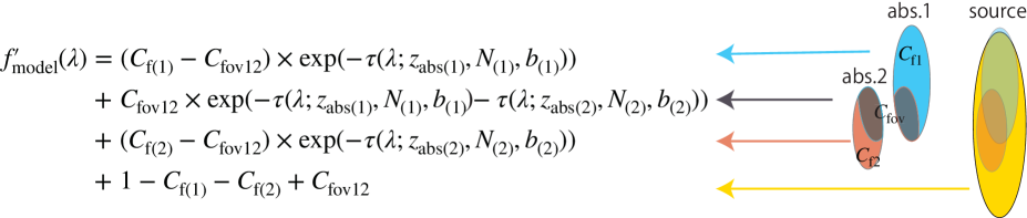
Figure 1.— Sketch of an absorption system with two components. If multiple clouds overlap along our line of sight to the background source, flux from the source is absorbed more than once. The number of parameters needed to fit the spectrum is $\left[\sum_{i=2}^{n}{n\choose i}\right]+4n$, and increases quickly with the number of components $n$.

The traditional $\chi^{2}$-based MINFIT fits models to the observed spectra by

$$f_{\rm mod}(\lambda) = \prod_{j=1}^{n}\left[C_{{\rm f}(j)}\times\exp{\{-\tau(\lambda;z_{{\rm abs}(j)},N_{(j)},b_{(j)})\}}\right.$$ (5)

$$\left.+1-C_{{\rm f}(j)}\right],$$

where $C_{{\rm f}(j)}$, $z_{{\rm abs}(j)}$, $N_{(j)}$, and $b_{(j)}$ are the parameters of component $j$. In equation (5), the overlap covering factor $C_{\rm fov}$ is not considered, but instead the brightness distribution of the background source, as seen by all absorbers along the cylinder of sight, is always uniform and the same, regardless of whether the absorbers overlap. This assumption is incorrect except for intervening absorbers where $C_{\rm f}$ = 1. Once we introduce $C_{\rm fov}$, the residual flux after being attenuated by two absorbing components for example would be written as

$$f_{\rm mod}^{\prime}(\lambda) = (C_{{\rm f}(1)}-C_{{\rm fov}(12)})$$ (6)

$$\hskip 14.22636pt\times\exp{(-\tau(\lambda;z_{{\rm abs}(1)},N_{(1)},b_{(1)}))}$$

$$+(C_{{\rm f}(2)}-C_{{\rm fov}(12)})$$

$$\hskip 14.22636pt\times\exp{(-\tau(\lambda;z_{{\rm abs}(2)},N_{(2)},b_{(2)}))}$$

$$+C_{{\rm fov}(12)}\times\exp\{(-\tau(\lambda;z_{{\rm abs}(1)},N_{(1)},b_{(1)})$$

$$\hskip 14.22636pt-\tau(\lambda;z_{{\rm abs}(2)},N_{(2)},b_{(2)}))\}$$

$$+1-C_{{\rm f}(1)}-C_{{\rm f}(2)}+C_{{\rm fov}(12)},$$

where $C_{{\rm fov}(12)}$ is the overlap covering factor between components 1 and 2. Since our code can accept any number of components, the total number of fit parameters for $n$ components is $\left[\sum_{i=2}^{n}{n\choose i}\right]+4n$ (where ${n\choose i}$ represents the number of possible combinations of $i$ items drawn from a set of $n$ items) after adding the overlap covering factors (the first term) to the original parameters for each component (the second term). However, it should be noted that total number of model parameters (and then the posterior distribution of them) would be quite large if we use a large number of components in the fit.

2.2. Fitting Procedure

Before using our MCMC-based VP fitting code (mc2fit, hereafter), we need the prior distribution of model parameters. Since no information is available in advance, we assume a uniform distribution between appropriate lower and upper limits of each parameter as the prior. We then apply mc2fit to absorption lines following the procedure below:

• We make an initial estimate of the values of the parameters for each absorption component (i.e., $z_{\rm abs}$, log$N$, $b$, and $C_{\rm f}$) except for the overlap covering factor $C_{\rm fov}$, using the $\chi^{2}$-based VP fit code MINFIT. The code automatically returns the minimum number of necessary components for fitting the absorption profile. From these we determine min($C_{\rm fov}$) and max($C_{\rm fov}$), used in equation (3).

• We start the MCMC sampling using the affine-invariant ensemble sampler proposed by Goodman & Weare (2010) in the model parameter space with a number of dimensions of $\left[\sum_{i=2}^{n}{n\choose i}\right]+4n$. When the sampling points (i.e., walkers; the default number is 256 in our calculations) move from the position of the roughly estimated values, we demand they should fulfill detailed balance.

• Once we confirm that the auto-correlation time has converged (i.e., the MCMC algorithm has also converged), we continue sampling until the effective sample size becomes $\geq$100,000.

• We finally obtain a probability distribution and its mode (i.e., the best fit value) for each parameter by projecting the total probability density distribution on each parameter axis.

2.3. Comparison of MCMC and $\chi^{2}$ methods

We compare the fitting efficiencies of the MCMC method and the traditional $\chi^{2}$ method as follows. For the latter, we use MINFIT. First, we synthesize spectra with two C IV absorption components whose line widths and column densities are close to the broad and narrow components in the mini-BAL system that we will discuss in the next section: $b$ = 200 km s^-1 and log($N$/cm^-2) = 15 for the former and $b$ = 20 km s^-1 and log($N$/cm^-2) = 14 for the latter, but both components have the same absorption redshift and covering factor ($z_{\rm abs}$ = 2.0 and $C_{\rm f}$ = 0.5). These parameters are kept fixed. But we do change overlap conditions as $C_{\rm fov\_norm}$ = 0, 0.25, 0.5, 0.75, and 1. A spectrum is synthesized from 4634Å to 4661Å with a pixel size of 0.03Å pixel^-1. As shown in Figure 2, the total absorption depth is deeper when $C_{\rm fov\_ratio}$ is smaller. Next, we convolve the spectrum with the appropriate line-spread function to simulate a spectral resolution of $\lambda/\Delta\lambda$ = 36,000, which is a typical values for observational data as is presented in Section 3. In fact, the convolution does not significantly affect the absorption profiles since both the broad and the narrow components are much broader than the spectral resolution element ($\Delta v$ $\sim$ 8.3 km s^-1). To examine how much the fitting accuracy would improve as the S/N increases, we synthesize spectra with different noise realizations with S/N from 10 to 100 pixel^-1 in steps of 10 and reproduce the fit parameters repeatedly.

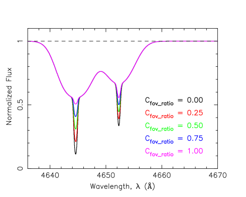
Figure 2.— Synthesized spectra with two C IV absorption components whose line parameters are log($N$/cm^-2) = 15, $b$ = 200 km s^-1, and $C_{\rm f}$ = 0.5 for the broader component, and log($N$/cm^-2) = 14, $b$ = 20 km s^-1, and $C_{\rm f}$ = 0.5 for the narrower component. The spectra with different $C_{\rm fov\_ratio}$ are overlaid in different colors. Even a synthesize spectrum with no overlap (i.e., black curve) does not reach zero flux at its center, since optical depth of two absorption components are not large enough to be saturated.

Once all the spectra are synthesized, we fit them with VP components using mc2fit and MINFIT, respectively. We repeat this analysis 10 times by changing the seed value of the random number generator (used for adding noise). Finally, we calculate the average and the standard deviation of best-fit (i.e., mode) values for each line parameter.

Figure 3 shows a comparison of fit parameters (log$N$, $b$, and $C_{\rm f}$) that are returned by mc2fit and MINFIT as a function of S/N. In this demonstration, we adopt $C_{\rm fov\_norm}$ = 0.5 (i.e., $C_{\rm fov}$ = 0.25 and $C_{\rm fov\_ratio}$ = 0.5). The code mc2fit always provides the correct values within 1$\sigma$ uncertainty, while MINFIT underestimates log$N$ and $b$ for the broad component even in high-quality spectrum with S/N = 100 pixel^-1. The discrepancy is probably a result of not allowing for an overlap covering factor in MINFIT. Thus, for cases where multiple absorbers overlap along the line of sight, the MCMC method is required to derive correct line parameters.

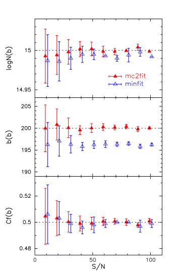
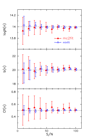
Figure 3.— Comparison of fit parameters for the synthesized spectra in Figure 2 (log$N$, $b$, and $C_{\rm f}$ from top to bottom) using mc2fit (red filled triangle) and MINFIT (blue open triangle) with 1$\sigma$ uncertainties (vertical solid line) as a function of S/N. The normalized covering factor is fixed to $C_{\rm fov\_norm}$ = 0.5. To facilitate comparison, the points are intentionally shifted horizontally. Horizontal dotted lines denote correct values. Left and right figures are results for the broad (b) and the narrow (n) components, respectively.

We also summarize the fit results of the overlap covering factor ($C_{\rm fov}$) and the overlap covering factor ratio ($C_{\rm fov\_ratio}$) by mc2fit in Figure 4 for some selected values, $C_{\rm fov}$ = 0.0, 0.125, 0.25, 0.375, 0.5, and $C_{\rm fov\_ratio}$ = 0.0, 0.25, 0.5, 0.75, 1.0. An example of a corner plot is also shown in Figure 5. The code recovers $C_{\rm fov\_ratio}$ generally well, while $C_{\rm fov}$ is always under-estimated even in spectra with S/N $\sim$ 100 pixel^-1 if the correct $C_{\rm fov}$ value is 0.5. Therefore, we will use $C_{\rm fov\_ratio}$ to examine whether absorbers overlap, since it is always determined reliably (at least the correct value is within 1$\sigma$ uncertainty) if the data quality is high enough, S/N $\geq$ 30 pixel^-1.

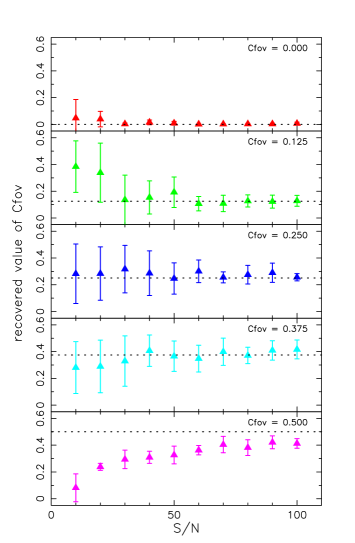
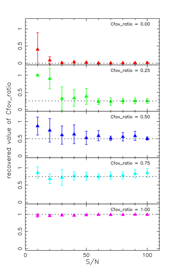
Figure 4.— Overlap covering factor ($C_{\rm fov}$, left) and overlap covering factor ratio ($C_{\rm fov\_ratio}$, right) that are reproduced by mc2fit (filled triangle) with 1$\sigma$ uncertainties (vertical solid line) as a function of S/N. The normalized covering factor is fixed as $C_{\rm fov\_norm}$ = 0.0, 0.25, 0.5, 0.75, and 1.0 from top to bottom (i.e., $C_{\rm fov}$ = 0.0, 0.125, 0.25, 0.375, 0.5 and $C_{\rm fov\_ratio}$ = 0.0, 0.25, 0.5, 0.75, 1.0). Horizontal dotted lines denote correct values.

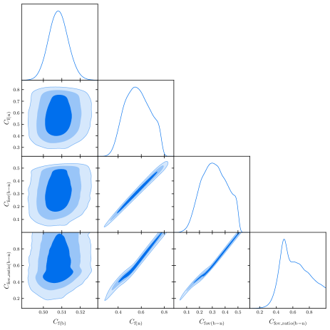
Figure 5.— Example of posterior probability distribution function of covering factors ($C_{\rm f}$, correct values are 0.5) of both broad and narrow components as well as their overlap covering factor ($C_{\rm fov}$, 0.25) and overlap covering factor ratio ($C_{\rm fov\_ratio}$, 0.5).

3. Application to Observed Spectra

To test mc2fit further, we apply it to a mini-BAL system whose line profile is easy to separate into multiple absorption components (i.e., an ideal target to test the code) that is detected in an optically bright quasar. There also exist several narrow absorption line systems in the same quasar spectrum.

3.1. Mini-BAL Quasar UM675

In the spectrum of the radio-loud luminous quasar UM675 at $z_{\rm em}$ = 2.147, Sargent et al. (1988) detected three C IV NALs at $z_{\rm abs}$ $\sim$ 1.7666, 1.9288, and 2.0083. Hamann et al. (1995) also discovered C IV, N V, and Ly$\alpha$ mini-BALs with FWHM $\sim~{}500~{}{{{\rm km~{}s}^{-1}}}$ with a high metallicity ($Z$ $>$ 2$Z_{\odot}$) at $z_{\rm abs}$ $\sim$ 2.134 corresponding to an offset velocity of $v_{\rm off}$ $\sim$1500 km s^-1 from the quasar emission redshift. The mini-BAL system is optically thin because the Lyman-continuum edge is absent. The system also has a wide variety of absorption lines with a full range of ionization from Ne VIII (ionization potential IP = 239 eV) to C III (IP = 48 eV) (Beaver et al., 1991; Hamann et al., 1995), which suggests that the gas density and/or radial distance from the flux source span a factor of $\sim$100 or $\sim$10, respectively.

Using intermediate-resolution spectra ($R$ $\sim$ 1500), Hamann et al. (1995) discovered time variability in the absorption strength of the C IV and N V mini-BALs in $\Delta t_{\rm rest}\sim 2.9$ years in the quasar rest-frame, and placed a lower limit on the electron density of $n_{\rm e}\geq 4000$ cm^-3 and an upper limit on the radial distance from the source of $r\leq 200$ pc, assuming the absorber is in ionization equilibrium. There is clear evidence for partial coverage of the background flux source ($C_{\rm f}$ = 0.63${}^{+0.2}_{-0.1}$ for N V and 0.34${}^{+0.1}_{-0.0}$ for C IV at $v_{\rm off}$ $\sim$1500 km s^-1; Hamann et al. 1997b) based on high resolution spectra taken with Keck/HIRES, which means the mini-BAL system is physically associated with the quasar (i.e., intrinsic QAL). Hamann et al. (1997b) also detected three narrow components with FWHM $\sim$ 30–50 km s^-1 inside the smooth mini-BAL profiles of C IV and N V, as shown in Figure 2 of their paper.

To date, high-resolution spectra ($R$ $\sim$ 35000 – 45000) of the quasar have been obtained three times with Keck/HIRES in 1994 September (hereafter, epoch E1), 1998 September (E2), and 2008 January (E4), and once with Subaru/HDS in 2005 August (E3) as summarized in Table 1. The spectrum in epoch E1 is shown here in Figure 6 as an example. Using the high-resolution spectra in epochs E1 and E3, Misawa et al. (2014) confirmed again that the absorption strengths (i.e., equivalent width) of Ly$\alpha$, C IV, and N V show an obvious time variability with $>$5$\sigma$ significance level, but with no discernible changes in the narrow components inside it. In this study, we use all of the above that are available from the Keck Observatory Archive (KOA) or obtained by us with Subaru/HDS although the N V mini-BAL is not covered by the spectrum in epoch E2. We reduced the data ourselves using a data reduction pipeline for Keck/HIRES data (MAuna Kea Echelle Extraction; MAKEE). After normalizing the spectra, we searched for absorption lines whose depth is greater than 5 times the corresponding noise level. We identified six C IV NALs at $z_{\rm abs}$ = 2.0569, 2.0083, 1.9288, 1.7663, 1.6769, and 1.6387 between the Ly$\alpha$ and C IV emission lines (Systems B, C, D, E, F and G, hereafter) in addition to the mini-BAL system at $z_{\rm abs}$ $\sim$ 2.134 (System A, hereafter), as summarized in Table 2. Among these, System C, D, and E were already reported in Sargent et al. (1988).

Table 1Log of Monitoring Observations

Epoch	Obs. Date	Instrument	$\lambda$-coverage	Exp. Time	$\lambda/\Delta\lambda^{a}$	S/N (N V)b	S/N (C IV)b	Source of Datac
			(Å)	(sec.)		(pixel-1)	(pixel-1)
E1	1994 Sep 24–25	Keck+HIRES	3750–6100	18000	34,000	47	9	A
E2	1998 Sep 22	Keck+HIRES	4150–6520	3600	47,800	d	16	B
E3	2005 Aug 19–20	Subaru+HDS	3600–5980	23000	36,000	48	28	C
E4	2008 Jan 15	Keck+HIRES	3200–5990	840	47,750	12	9	B

Table 2Absorption Line Systems

System	$z_{\rm abs}$	$v_{\rm off}$a	Classb	Ionsc	Variabilityd
		(km s-1)
A	$\sim$2.134	$\sim$1,240	mini-BAL	C IV, N V, (Ly$\alpha$)	Y
B	2.0569	8,710	NAL	C IV	N
Ce	2.0083f	13,510	NAL	C IV, Si IV, (C II)	N
D	1.9288	21,520	NAL	C IV, Si IV, (Si II)	N
E	1.7663	38,470	NAL	C IV	N
F	1.6769	48,120	NAL	C IV	N
G	1.6387	52,310	NAL	C IV	N

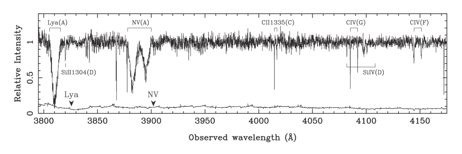
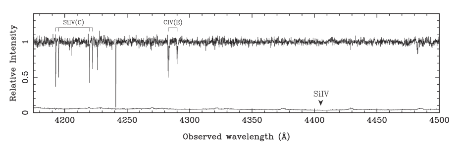
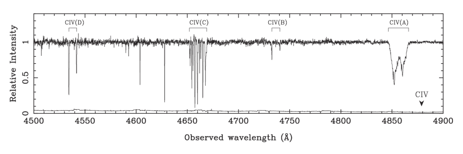
Figure 6.— Normalized spectrum of UM675 after rebinning to 0.1 Å per pixel. The C IV, N V, Si IV doublets and other detected single lines are marked. Positions of the quasar emission lines of Ly$\alpha$, N V, Si IV, and C IV are marked with downward arrows. The regions blueward of the Ly$\alpha$ absorption in system A and redward of the C IV emission line are not shown. The lower trace shows the 1$\sigma$ error spectrum.

3.2. MCMC fit to a mini-BAL and six NALs

We use mc2fit to fit the C IV and N V mini-BALs and six C IV NALs in the spectra of UM675 in the four epochs. As a prior, we assume a uniform distribution between the lower and upper limits of each parameter: [1.469, 2.147] (i.e., between the redshift of C IV absorption line corresponding to the Ly$\alpha$ emission line and the quasar emission redshift) for $z_{\rm abs}$, (0, 16] for log($N$/cm^-2), (0, 2000) (i.e., the boundary between BAL and mini-BAL) for $b$ [km s^-1], (0, 1] for $C_{\rm f}$, and (0, 1] for $C_{\rm fov\_norm}$, where parentheses, (a, b), and square brackets [a, b] denote an interval from a to b, but only the latter includes the values of a and b themselves. The best-fit models are presented in Figure 7.

Figure 7.— Best-fit models for the C IV and N V mini-BALs in System A using the MCMC method. The velocity on the horizontal axis is defined relative to the flux-weighted center of the absorption profiles. The top and middle panels show the profiles of the blue and red members of a doublet on a common velocity scale, with the model profile produced by mc2fit superposed: dashed lines for each component and a solid line for the contribution of all components. The bottom panel shows the two profiles together, along with the resulting covering factors (open circles) with their 1$\sigma$ error bars. Profiles in the shaded areas are ignored for fitting. The complete figure set is available in Appendix.

We confirm that only the mini-BAL system (i.e., System A) shows statistically significant partial coverage in both C IV and N V profiles, while none of the NAL systems show partial coverage with $>3\sigma$ confidence level (i.e., the NAL systems are probably intervening QALs). Therefore, we will study the fit parameters only for System A. The best fit parameters for System A and their 1$\sigma$/3$\sigma$ uncertainties are summarized for all epochs in Table 3. Included are the absorption redshift, column density, Doppler parameter, covering factor, and rest-frame equivalent width. We present the fitting results of the NAL systems (i.e., Systems B – G) in Table 4, but only for epoch E1 since there is no variability. In the following, we describe the results for each system in detail.

3.3. System A

We clearly detect C IV and N V mini-BALs at $z_{\rm abs}$ $\sim$ 2.134 but Si IV is not detected in the corresponding region ($\lambda$ $\sim$ 4400 Å). Figure 8 shows normalized spectra around the C IV and N V mini-BALs for all four epochs, which clearly indicate the system is variable. Although Hamann et al. (1997b) detected three narrow components within a broad absorption feature in the C IV and N V mini-BALs in epoch E1, we consider only two narrow components because the third (weakest) component in Hamann et al. (1997b) is very weak and almost swamped in the noise around the N V mini-BAL in the same epoch and in the C IV mini-BAL in all other epochs. Hereafter, we refer to them as components b (broad), n1 (narrow 1; at longer wavelength), and n2 (narrow 2; at shorter wavelength), respectively, as shown in Figure 9, where the best fit model is superposed for comparison.

Figure 8.— Normalized spectra around the C IV (top) and N V (bottom) mini-BALs in system A. Vertical axis denotes normalized flux. Horizontal axis denotes the offset velocity of the flux-weighted center of the blue member of the doublet (i.e., C IV $\lambda$1548 and N V $\lambda$1239) from the quasar. The first to fourth epoch spectra are shown with blue, orange, green, and red histograms.

Figure 9.— Best fit model to the normalized C IV and N V mini-BALs (System A) in the quasar UM675 in epoch E1. The observed (blue histogram) and modeled (black curve) spectra around C IV 1548, C IV 1551, N V 1239, and N V 1243 are shown from the top to the bottom as a function of offset velocity from the quasar emission redshift. Orange, green, and red dashed curves are the best models for components b, n1, and n2, respectively. The horizontal axis is offset velocity from the quasar emission redshift, while the vertical axis is normalized flux. Absorption lines in the shaded areas at $v_{\rm off}$ $\sim$ 850 km s^-1 and 1650 km s^-1 in the third panel are unrelated profiles.

We find significant variability at $>$3$\sigma$ confidence level in $C_{\rm f}$ of component b both in the C IV and the N V mini-BALs as well as in $b$ of component b only in the N V mini-BAL (see Table 3 and Figure 10) In contrast, all parameters of components n1 and n2 are stable over all epochs at the $3\sigma$ level.

Figure 10.— Variation of fit parameters with time (log$N$, $b$, and $C_{\rm f}$ from the top to the bottom) of component b in C IV (left) and N V (right) mini-BALs. Horizontal axis gives relative time from the first observing epoch (i.e., epoch E1) in the quasar rest-frame. Black dots show the mode of fit parameter posterior distributions, while black and red error bars denote 1$\sigma$ and 3$\sigma$ uncertainties. Only $C_{\rm f}$ shows $>3\sigma$ variability in C IV mini-BAL, while $C_{\rm f}$ and $b$ vary in the N V mini-BAL.

We also study the overlap covering factor ratio ($C_{\rm fov\_ratio}$) between components b and n1/n2. We placed the strongest constraints on $C_{\rm fov\_ratio}$ in the E3 spectrum. As shown in Figure 11, components b ($C_{\rm f}$ = 0.33$\pm$0.01) and n1 ($C_{\rm f}$ = 0.52${}^{+0.02}_{-0.04}$) in the C IV mini-BAL are found to overlap by at least 50% of the projected size of the smaller component (i.e., component b) since the $3\sigma$ lower limit on $C_{\rm fov\_ratio}$ is $\sim$0.54. Thus, for the first time we find with high confidence that multiple absorbing clouds along our line of sight overlap with each other. However, there need not be overlap between b and n1 for N V, since we found a $3\sigma$ upper limit on $C_{\rm fov\_ratio}$ of $\sim$0.69 for the N V mini-BAL (see Figure 11). That is, in the case of Figure 1 the two C IV absorbers should overlap along our line of sight by at least 50% of their size, while the two N V absorbers do not necessarily overlap. Here, we should emphasize that the C IV and N V absorbers do not necessarily have an identical overlap covering factor ratio because they may represent different layers in the absorber (i.e., they have different covering factors).

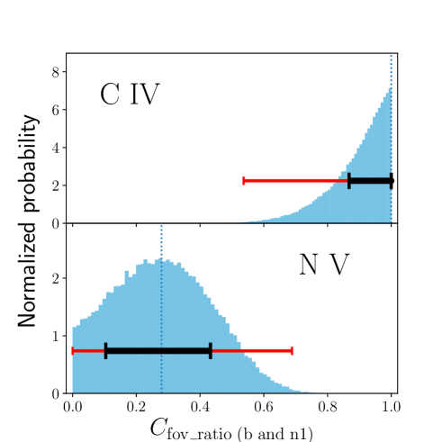
Figure 11.— Probability distribution histogram of $C_{\rm fov\_ratio}$ between components b and n1 in epoch E3 for C IV (top) and N V (bottom). Vertical dotted lines are modes of the $C_{\rm fov\_ratio}$. Horizontal black and red error bars denote 1$\sigma$ and 3$\sigma$ uncertainties.

3.4. System B

We detect only a weak C IV NAL with $EW_{\rm rest}\sim 0.03$ Å in the system. The covering factor is $C_{\rm f}$ = 1, which suggests an intervening absorber. A weak absorption profile on the left side of the blue component is not part of C IV $\lambda$1548 since we do not find any absorption features in the C IV $\lambda$1551 window. Therefore, we ignore this region when carrying out the fit. The best fit model is shown in Figure 7.

3.5. System C

There are five components in C IV and two in Si IV in this system, of which some are completely separated from each other by unabsorbed spectral regions. However, we regard these components as a single NAL system since their overall velocity separation is $<$ 200 km s^-1 from each other, following Misawa et al. (2007a). The best fit model is presented in Figure 7. The fit to component 1 of the Si IV NAL implies partial coverage ($C_{\rm f}$ $\sim$ 0.69) with a 3$\sigma$ confidence level. However, this result should be regarded with caution because (i) there exist narrow spikes in both the blue and red members of the Si IV doublet that could be due to data defects and (ii) the best-fit model appears to overestimate the depth of red component which would underestimate $C_{\rm f}$. The $C_{\rm fov\_ratio}$ between components 4 and 5 in the C IV NAL is consistent with unity, which is reasonable since both components have full coverage.

3.6. System D

We detect C IV and Si IV NALs in this system. We fit models with two components to the C IV NAL because of its asymmetric profile, while a single component model is acceptable for the Si IV NAL (see Figure 7). All components are consistent with full coverage at the 1$\sigma$ confidence level. It is reasonable that $C_{\rm fov\_ratio}$ $\sim$ 1 between the two components of the C IV NAL since both have full coverage.

3.7. System E

We detect only a C IV NAL that consists of two components. Both components are consistent with full coverage at the 3$\sigma$ level. There could exist a third very weak component at $\Delta~{}v$ $\sim$ 60 km s^-1 in Figure 7, but we ignore it since it is not detected with $>$ 5$\sigma$ confidence (i.e., does not satisfy our detection criterion).

3.8. System F

A shallow and broad C IV NAL with a Doppler parameter of $b$ $\sim$ 23 km s^-1 is detected in the system as shown in Figure 7. The system is probably an intervening absorber, since $C_{\rm f}$ $\sim$ 1 at the 3$\sigma$ confidence level.

3.9. System G

Only a C IV NAL is detected in this system. Although we fit a model with a single component to this NAL, there could be two components since the C IV $\lambda$1548 profile is slightly asymmetric. For multi-component fitting, we would need a higher S/N spectrum. The covering factor is consistent with full coverage. The best-fit models are presented in Figure 7.

4. Discussion

4.1. Possible Geometry

Using the MCMC-based method for fitting the mini-BALs in the spectrum of UM675, we find for the first time that multiple absorbing clouds (i.e., components b and n1) overlap along our line of sight to the background flux source, which could not have been inferred with the $\chi^{2}$-based method. Thus, the projected distribution of integrated total column density from multiple absorbing clouds along the line of sight is much more complex than previously thought. By synthesizing artificial spectra, Sabra & Hamann (2005) studied how the column density that we derive from the observed spectrum depends on inhomogeneous partial coverage. They found that homogeneous and inhomogeneous models have little difference (apparent optical depths within 50%) as long as the column density distribution does not contain spatially narrow peaks (i.e., large enhancements in the optical depth over small coverage areas).

The fits to the C IV and the N V mini-BALs in epoch E3 provide the strongest constraints on partial coverage among the four epochs because of the high S/N in that spectrum; $C_{\rm f}$ _(b) = 0.33${}^{+0.01}_{-0.01}$, $C_{\rm f}$ _(n1) = 0.52${}^{+0.02}_{-0.04}$, and $C_{\rm f}$ _(n2) = 0.38${}^{+0.04}_{-0.11}$ for components b, n1, and n2 of the C IV mini-BAL, and $C_{\rm f}$ _(b) = 0.49${}^{+0.02}_{-0.02}$, $C_{\rm f}$ _(n1) = 0.16${}^{+0.02}_{-0.02}$, and $C_{\rm f}$ _(n2) = 0.83${}^{+0.17}_{-0.60}$ for those of the N V mini-BAL, respectively. All components (except for component n2 of the N V mini-BAL) show partial coverage with a confidence $>3\sigma$. The width of component b (FWHM $\sim$200 km s^-1) is much larger than those of narrow components (FWHM $\sim$10–30 km s^-1), which suggests that only component b has a large velocity dispersion possibly due to mechanisms such as internal turbulence or continuous acceleration, but that its transverse scale is comparable to those of the narrow components.

We also noticed that $C_{\rm f}$ (N V) is always larger than $C_{\rm f}$ (C IV) in all epochs for component b. This trend (i.e., higher ions tend to have larger covering factors) is consistent with other reports in the literature (e.g., Petitjean & Srianand 1999; Srianand & Petitjean 2000; Misawa et al. 2007a; Muzahid et al. 2016), suggesting that the size of the N V absorbers is larger than that of the C IV absorbers and/or the effective size of flux source behind the N V absorber is smaller than that behind the C IV absorber (cf. Figure 1). Interestingly, the opposite is true for components n1 and n2; i.e., $C_{\rm f}$ (N V) tends to be smaller than $C_{\rm f}$ (C IV) as shown in Figure 12. This discrepancy between the broad and the narrow components suggests that the size (or flux amplitude) of the background flux source is different between N V and C IV absorbers. This could happen for the narrow components if the N V absorption line is more diluted than the C IV absorption line by the flux from the BELR whose scale ($\sim$0.1 pc; Hamann et al. 1997b and references therein) is $\sim$2 orders of magnitude larger than the size of the continuum source as we will discuss later. Because both the C IV and N V mini-BALs are located on the blue wing of the corresponding broad emission lines (see Figure 1 of Hamann et al. 1995), their depths can be diluted by the broad emission line flux (e.g., Arav et al. 1999).

Figure 12.— Difference between $C_{\rm f}$ (N V) and $C_{\rm f}$ (C IV) of components b (blue) and n1 (red) as a function of relative time from the first epoch in the quasar rest frame. Black dots are modes of the difference. Black and blue/red error bars denote 1$\sigma$ and 3$\sigma$ uncertainties of the difference. The dots with error bars are intentionally shifted by $\pm$0.05 years from the observed epoch in the horizontal direction for display purpose.

Considering contributions from both the continuum source and the BELR, we can calculate the total covering factor $C_{\rm f}$ by

$$C_{\rm f}=\frac{C_{\rm f(cont)}+W\times C_{\rm f(BELR)}}{1+W},$$ (7)

where $C_{\rm f(cont)}$ and $C_{\rm f(BELR)}$ are covering factors of the continuum source and BELR and $W$ (= $F_{\rm BELR}/F_{\rm c}$) is defined as the ratio of the fluxes from the BELR ($F_{\rm BELR}$) and the continuum source ($F_{\rm c}$) (Ganguly et al., 1999). Indeed, the flux ratio ($W$) around the N V mini-BAL due to the contribution from both Ly$\alpha$ and N V broad emission lines is obviously larger than that around the C IV mini-BAL (see Figure 1 of Hamann et al. 1995). Thus, the opposite trend of the ratio of $C_{\rm f}$ (C IV) and $C_{\rm f}$ (N V) in components b and n1/n2 can be due to a difference in the contribution from the background flux source, as discussed in Wu et al. (2010).

We speculate that component b does not absorb light from the BELR (it may be at smaller radial distance than the BELR, $r$ $\leq$ 0.1 pc or embedded within it), while components n1 and n2 also absorb light from the BELR (possibly because they are located at a larger radial distance); we refer to this scenario as model A, hereafter. The very high ionization state of the gas in component b, showing Ne VIII and O VI, also supports its small radial distance from the continuum source. In other words, components b and n1/n2 are not co-spatial but happen to be located along the same cylinder of sight with a similar offset velocity perhaps due to line-locking. Just as in the UM675 spectrum, narrow kinematic components are sometimes detected near the centers of mini-BALs in other quasars (e.g., HE1341$-$1020, Q1157$+$014, and Q2343$+$125) and they usually show no variability while broader components vary (Hamann et al., 1997a; Misawa et al., 2014). Possible origins of these narrow components include (i) dense clumpy clouds with large volume density (i.e., less affected by fluctuation of incident flux) embedded in the mini-BAL flow (Misawa et al., 2014) and (ii) gas clouds in the quasar host galaxy or in foreground galaxies that are physically unrelated to the quasar (Hamann et al., 1997a). In addition to these, we propose a third possible origin: (iii) dense clumpy clouds with large volume density whose radial distance is a few orders of magnitude larger than the mini-BAL flow (e.g., Itoh et al. 2020) but with their radial velocity coinciding. The variety of absorption lines with a wide range of ionization potential (Beaver et al., 1991; Hamann et al., 1995) also supports this idea.

Although the above scenario is possible, it is unlikely that the broad and narrow absorbers at very different distances have similar velocities relative to the quasar by chance. In that spirit, we present an alternative model, model B, hereafter, in which the broad and the narrow absorbers coexist at the same radial distance. In this model, most of the absorber has relatively a low density and high ionization state and large velocity gradient (corresponding to component b). Within the large gas parcel there are dense clumps with low ionization state and small velocity gradient (corresponding to components n1 and n2). The entire absorber is moving both in the transverse and radial directions as it orbits around the flux sources. The size of component b is comparable to the size of the continuum source so that it can partially cover both the continuum source and the BELR. With this geometry, components n1 and n2 can also produce partial coverage since they are smaller than component b.

In either model, the geometry of the mini-BAL system in UM675 requires two distinct flux sources (i.e., the continuum source and BELR), while mc2fit (as well as other $\chi^{2}$-based codes) assumes a single background flux source. To verify this geometry, we need to introduce covering factors ($C_{\rm f}$) and their overlap covering factor ratios ($C_{\rm fov\_ratio}$) as free parameters for both background flux sources individually, or introduce a model for the brightness distribution of the background flux source(s) and then adopt specific geometrical arrangements for the absorbers, or both. However, the current version of mc2fit does not have these features. These are improvements that we will introduce in a future version of the code.

One possible observational test to distinguish between models A and B is through monitoring of the outflow velocity of the narrow components. In model B, components n1 and n2 should show a velocity shift on a time scale similar to the dynamical (i.e., crossing) time of the BELR, $t_{\rm dyn}$ since they are located at a radial distance comparable to the size of the BELR. Assuming a Keplerian motion, we derive $t_{\rm dyn}$ $\sim$23 years in the quasar’s rest frame which is much longer than our current monitoring period of $\sim$4.24 years.

4.2. Origin of Time Variability

In addition to the variability in absorption strength (Hamann et al., 1995; Misawa et al., 2014), we also find variability in the line parameters of the mini-BAL system: component b shows $>3\sigma$ variability in $C_{\rm f}$ of the C IV mini-BAL and in both $C_{\rm f}$ and $b$ of the N V mini-BAL in $\sim$4.24 years in the quasar’s rest frame. Since the time separation between epochs E3 and E4 is the smallest ($\Delta t_{\rm rest}$ $\sim$0.77 year) among the four observing epochs, we concentrate on the variability pattern on that short time interval since it can place the most stringent constraints on the physical conditions of the absorbers.

There are two major scenarios for the origin of time variability that have often been discussed in the literature: (1) a change of the ionization state of the gas clouds (e.g., Misawa et al. 2007b; Hamann et al. 2011; Filiz Ak et al. 2013; Horiuchi et al. 2016) and (2) motion of the absorbing clouds across our line of sight to the background flux source (e.g., Gibson et al. 2008; Hamann et al. 2008; Vivek et al. 2016; Krongold et al. 2017). Neither situation is applicable to intervening absorbers, unless they have very large gas density and/or sharp edges (Narayanan et al., 2004).

The column densities of component b in the C IV and N V mini-BALs are almost constant while their $C_{\rm f}$ values vary (see Figure 10), which supports the gas motion scenario. To examine this scenario, we first need to estimate the sizes of the background flux sources (i.e., the continuum source and BELR). Following Misawa et al. (2005), we take five times the gravitational radius as the continuum source size using a black hole mass of $\log(M_{\rm BH}/M_{\odot})$ = 9.52 (Horiuchi et al., 2016). For the size of the portion of the BELR that emits the C IV line, we use equation (1) of Lira et al. (2018) with Galactic extinction of $A_{V}$ = 0.44 and assume a power-law index of $\alpha$ = 0.61 (Lusso et al., 2015). We obtain $R_{\rm cont}$ $\sim$ $2\times 10^{-3}$ pc and $R_{\rm BELR}$ $\sim$ $0.2$ pc as the sizes of the continuum source and the BELR, respectively.

Since component b of the C IV mini-BAL shows variability in covering factor from $C_{\rm f}$ = 0.33${}^{+0.01}_{-0.01}$ to 0.42${}^{+0.03}_{-0.02}$ in $\Delta t_{\rm rest}$ = 0.77 years, we can place a lower limit on the crossing velocity as $v_{\rm cross}\geq d_{\rm s}\times\Delta C_{\rm f}/\Delta t_{\rm rest}$, where $d_{\rm s}$ is the size of the continuum source $d_{\rm cont}$ (or the size of the absorber $d_{\rm abs}$) if $d_{\rm abs}$ is larger (or smaller) than $d_{\rm cont}$ respectively. We adopt $\Delta C_{\rm f}=0.09$ as the variability amplitude of $C_{\rm f}$, and take $\Delta t_{\rm rest}$ to be the time interval between observing epochs in the quasar’s rest frame. Since we want to place a lower limit on $v_{\rm cross}$, we should use a smaller size between $d_{\rm abs}$ and $d_{\rm cont}$ (i.e., $d_{\rm s}$ = min{$d_{\rm abs},d_{\rm cont}$}). However, these sizes should be almost the same since the absorber shows partial coverage, which leads us to use $d_{\rm s}$ $\sim$ $d_{\rm cont}$ whose value we have been able to estimate. Substituting the values above into $d_{\rm cont}\times\Delta C_{\rm f}/\Delta t_{\rm rest}$, we obtain $v_{\rm cross}$ $\geq$ 366 km s^-1. If the crossing velocity is equal to the Keplerian orbital velocity around the central black hole, we can also place a weak constraint on the absorber’s radial distance from the flux source as $\leq$ 106 pc for component b. We also note that in the context of model A this radial distance is probably smaller than the size of BELR ($<$ $R_{\rm BELR}$ $\sim$ 0.2 pc) as discussed above.

In comparison, components n1 and n2 do not show significant (i.e., $>3\sigma$) variability during our monitoring campaign in $\Delta t_{\rm rest}$ = 4.24 years. Therefore, we cannot place any constraints on either crossing velocity or radial distance.

5. Summary

In this study, we introduce a Bayesian approach combined with an MCMC method for fitting a mini-BAL and six NAL systems in the spectrum of a radio-loud quasar UM675 taken with Keck/HIRES and Subaru/HDS in four epochs. Our methodology is implemented in a new code, mc2fit, which we test here using synthetic and real spectra. Our main results are as follows:

• Using mc2fit, we restrict the range of covering factor ($C_{\rm f}$) from 0 to 1 as is physically possible and determine the fit parameters more accurately than the traditional $\chi^{2}$-based methods. Our fitting results for synthetic spectra are fairly consistent with those obtained by the $\chi^{2}$-based method described in Misawa et al. (2007a), but the latter method slightly underestimate log$N$ and $b$ compared to the correct values.

• In addition to the original fit parameters (i.e., $z_{\rm abs}$, log$N$, $b$, $C_{\rm f}$), we introduce the overlap covering factor ratio by multiple absorbers along our line of sight ($C_{\rm fov\_ratio}$). Because of the large number of fit parameters ($\left[\sum_{i=2}^{n}{n\choose i}\right]+4n$ in total for $n$ components), any observed spectrum to which we apply mc2fit must have a very high S/N. Otherwise, the code tends to overestimate $C_{\rm fov\_ratio}$ especially when the correct value is small.

• Among seven absorption systems (Systems A – G) in the quasar UM675, only the C IV and N V mini-BALs at $z_{\rm abs}$ $\sim$ 2.1341 (System A) show clear simultaneous variability in their $C_{\rm f}$ and $b$ at $>3\sigma$ confidence level. We also determine for the first time that multiple absorbing clouds (i.e., the broad and the narrow components) overlap each other along our line of sight.

• For component b of the mini-BAL system (System A), $C_{\rm f}$ (N V) is always larger than $C_{\rm f}$ (C IV) at all epochs, while the opposite trend holds for components n1 and n2. These trends suggest that the broad component does not absorb light from the BELR or that the narrow components do not absorb light from the continuum source, depending on the possible models we have considered.

• The column densities of component b in the C IV and N V mini-BALs are almost constant while their $C_{\rm f}$ values vary, which supports the gas motion scenario for their variability. If this is the case, the broad component must be at $r<106$ pc (and could be closer than the size of $R_{\rm BELR}$, $\sim$ 0.2 pc) with a rotational velocity of $v_{\rm rot}>366$ km s^-1 assuming Keplerian motion (we cannot place any meaningful constraints for the narrow components).

The MCMC-based approach improves fitting results significantly compared to the traditional $\chi^{2}$-based methods especially for high-quality spectra with S/N $\geq$ 30 pixel^-1. It also provides the overlap covering factor ratio ($C_{\rm fov\_ratio}$) if multiple components overlap in the spectrum, which conveys important information on the absorber’s geometry. More detailed information can be obtained if we introduce fit parameters for the continuum source and BELR, separately. To capitalize on the MCMC-based technique, we plan to monitor several mini-BAL systems whose absorption profiles are easy to de-blend using high quality spectra like the one in UM675.

Appendix

Best-fit models for absorption lines in Systems B – G using the MCMC method. The velocity on the horizontal axis is defined relative to the flux-weighted center of the absorption profiles. The top and middle panels show the profiles of the blue and red members of a doublet on a common velocity scale, with the model profile produced by mc2fit superposed: dashed lines for each component and a solid line for the contribution of all components. The bottom panel shows the two profiles together, along with the resulting covering factors (open circles) with their 1$\sigma$ error bars. Profiles in the shaded areas are ignored for fitting.

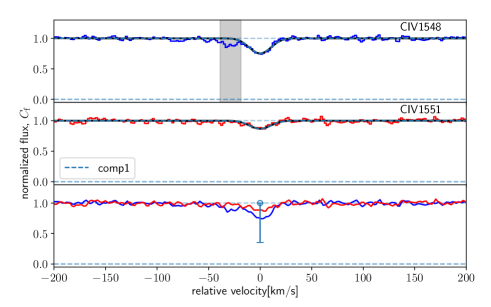
Figure 7.— Best-fit model for the C IV NAL in System B using the MCMC method.

Figure 7.— Best-fit models for the C IV and Si IV NALs in System C using the MCMC method.

Figure 7.— Best-fit models for the C IV and Si IV NALs in System C using the MCMC method.

Figure 7.— Best-fit models for the C IV and Si IV NALs in System D using the MCMC method.

Figure 7.— Best-fit model for the C IV NAL in System E using the MCMC method.

Figure 7.— Best-fit model for the C IV NAL in System F using the MCMC method.

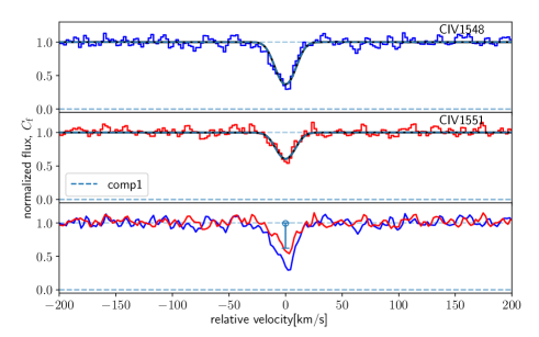
Figure 7.— Best-fit model for the C IV NAL in System G using the MCMC method.

Table 3Fitting Parameters of mini-BAL System in All Epochs

Ion	Epoch	comp.	$z_{\rm abs}$	$\log{N}^{a}$	$b^{a}$	$C_{\rm f}$a	$C_{\rm fov\_ratio}$a,b	EW${}_{\rm rest}^{c}$
				(cm-2)	(km s-1)			(Å)
System A
C IV	1	b	2.1344	$15.07_{-0.01(-0.04)}^{+0.01(+0.04)}$	$191.3_{-1.4(-4.0)}^{+1.3(+4.0)}$	$0.42_{-0.01(-0.02)}^{+0.01(+0.02)}$		$1.72\pm 0.07$
		n1	2.1341	$14.12_{-0.15(-0.33)}^{+0.09(+0.21)}$	$28.2_{-1.3(-3.7)}^{+1.4(+3.8)}$	$0.31_{-0.08(-0.12)}^{+0.18(+0.43)}$	$0.40_{-0.25(-0.39)}^{+0.24(+0.60)}$
		n2	2.1334	$13.62_{-0.11(-0.31)}^{+0.22(+0.69)}$	$12.7_{-1.2(-3.9)}^{+1.1(+3.2)}$	$0.52_{-0.23(-0.40)}^{+0.05(+0.14)}$	$0.65_{-0.11(-0.62)}^{+0.35(+0.35)}$
	2	b	2.1347	$14.95_{-0.07(-0.23)}^{+0.06(+0.18)}$	$204.3_{-6.3(-18.0)}^{+6.7(+21.0)}$	$0.40_{-0.03(-0.07)}^{+0.04(+0.16)}$		$1.47\pm 0.17$
		n1	2.1341	$13.96_{-0.26(-0.37)}^{+0.15(+0.47)}$	$30.9_{-2.5(-7.1)}^{+2.8(+8.6)}$	$0.66_{-0.18(-0.39)}^{+0.16(+0.34)}$	$1.00_{-0.36(-0.98)}^{+0.00(+0.00)}$
	3	b	2.1343	$14.98_{-0.02(-0.06)}^{+0.02(+0.06)}$	$193.0_{-1.9(-5.8)}^{+2.0(+6.2)}$	$0.33_{-0.01(-0.02)}^{+0.01(+0.03)}$		$1.22\pm 0.06$
		n1	2.1341	$14.13_{-0.03(-0.10)}^{+0.04(+0.13)}$	$25.6_{-0.6(-1.9)}^{+0.6(+1.8)}$	$0.52_{-0.04(-0.14)}^{+0.02(+0.04)}$	$1.00_{-0.13(-0.46)}^{+0.00(+0.00)}$
		n2	2.1334	$13.58_{-0.13(-0.40)}^{+0.15(+0.95)}$	$10.3_{-1.2(-4.7)}^{+1.3(+4.3)}$	$0.38_{-0.11(-0.28)}^{+0.04(+0.11)}$	$1.00_{-0.30(-0.91)}^{+0.00(+0.00)}$
	4	b	2.1345	$14.97_{-0.06(-0.20)}^{+0.06(+0.16)}$	$211.6_{-6.8(-19.5)}^{+6.8(+22.5)}$	$0.42_{-0.02(-0.06)}^{+0.03(+0.13)}$		$1.57\pm 0.30$
		n1	2.1341	$14.34_{-0.14(-0.34)}^{+0.31(+1.61)}$	$32.9_{-6.2(-16.4)}^{+4.2(+13.4)}$	$0.51_{-0.27(-0.36)}^{+0.03(+0.11)}$	$0.69_{-0.13(-0.67)}^{+0.31(+0.31)}$
N V	1	b	2.1343	$15.02_{-0.05(-0.16)}^{+0.04(+0.13)}$	$242.6_{-5.5(-16.0)}^{+5.4(+17.3)}$	$0.75_{-0.05(-0.13)}^{+0.06(+0.23)}$		$1.96\pm 0.33$
		n1	2.1341	$14.81_{-0.40(-0.90)}^{+0.55(+1.19)}$	$17.3_{-4.2(-7.9)}^{+5.6(+17.4)}$	$0.28_{-0.07(-0.17)}^{+0.07(+0.50)}$	$1.00_{-0.21(-0.93)}^{+0.00(+0.00)}$
		n2	2.1334	$13.53_{-0.18(-0.30)}^{+0.44(+2.45)}$	$9.9_{-2.9(-7.4)}^{+2.9(+9.4)}$	$0.24_{-0.06(-0.10)}^{+0.67(+0.76)}$	$1.00_{-0.39(-1.00)}^{+0.00(+0.00)}$
	3	b	2.1343	$14.96_{-0.03(-0.10)}^{+0.03(+0.08)}$	$196.5_{-2.3(-6.7)}^{+2.4(+7.2)}$	$0.49_{-0.02(-0.06)}^{+0.02(+0.09)}$		$1.05\pm 0.11$
		n1	2.1341	$15.48_{-0.25(-0.69)}^{+0.37(+0.52)}$	$15.1_{-0.8(-1.9)}^{+2.2(+6.8)}$	$0.16_{-0.02(-0.03)}^{+0.02(+0.07)}$	$0.28_{-0.18(-0.28)}^{+0.15(+0.41)}$
		n2	2.1334	$12.98_{-0.11(-0.23)}^{+0.32(+1.44)}$	$8.6_{-1.3(-4.2)}^{+1.4(+4.4)}$	$0.83_{-0.60(-0.72)}^{+0.17(+0.17)}$	$1.00_{-0.87(-1.00)}^{+0.00(+0.00)}$
	4	b	2.1342	$14.78_{-0.04(-0.07)}^{+0.07(+0.22)}$	$226.8_{-5.0(-15.9)}^{+4.8(+14.5)}$	$0.88_{-0.07(-0.24)}^{+0.10(+0.12)}$		$1.45\pm 0.49$
		n1	2.1340	$14.00_{-0.27(-0.48)}^{+0.36(+1.88)}$	$24.3_{-4.1(-14.2)}^{+3.9(+11.6)}$	$0.29_{-0.09(-0.14)}^{+0.32(+0.71)}$	$1.00_{-0.16(-1.00)}^{+0.00(+0.00)}$

Table 4Fitting Parameters of NAL Systems in epoch E1

Ion	comp.	$z_{\rm abs}$	$\log{N}^{a}$	$b^{a}$	$C_{\rm f}$a	$C_{\rm fov\_ratio}$a,b	EW${}_{\rm b\_rest}^{c}$
			(cm-2)	(km s-1)			(Å)
System B
C IV	1	2.0569	$13.00_{-0.04(-0.09)}^{+0.15(+0.52)}$	$13.2_{-0.9(-2.6)}^{+1.0(+3.3)}$	$1.00_{-0.30(-0.65)}^{+0.00(+0.00)}$		$0.03\pm 0.01$
System C
C IV	1	2.0063	$13.39_{-0.02(-0.05)}^{+0.05(+0.18)}$	$7.5_{-0.3(-0.9)}^{+0.3(+0.9)}$	$1.00_{-0.08(-0.22)}^{+0.00(+0.00)}$		$0.06\pm 0.00$
	2	2.0071	$13.08_{-0.03(-0.08)}^{+0.11(+0.38)}$	$6.8_{-0.5(-1.5)}^{+0.5(+1.6)}$	$0.99_{-0.19(-0.46)}^{+0.01(+0.01)}$		$0.04\pm 0.00$
	3	2.0083	$14.00_{-0.03(-0.08)}^{+0.03(+0.11)}$	$9.0_{-0.2(-0.6)}^{+0.2(+0.6)}$	$0.96_{-0.02(-0.05)}^{+0.02(+0.04)}$		$0.13\pm 0.01$
	4	2.0099	$13.80_{-0.02(-0.04)}^{+0.04(+0.14)}$	$23.6_{-0.5(-1.6)}^{+0.5(+1.7)}$	$1.00_{-0.07(-0.22)}^{+0.00(+0.00)}$		$0.17\pm 0.01^{d}$
	5	2.0100	$13.32_{-0.08(-0.19)}^{+0.12(+2.27)}$	$2.7_{-0.6(-1.7)}^{+0.6(+1.6)}$	$1.00_{-0.08(-0.36)}^{+0.00(+0.00)}$	$1.00_{-0.02(-0.22)}^{+0.00(+0.00)}$
Si IV	1e	2.0083	$13.49_{-0.13(-0.34)}^{+0.18(+1.33)}$	$5.9_{-0.6(-2.4)}^{+0.5(+1.4)}$	$0.69_{-0.03(-0.08)}^{+0.04(+0.15)}$		$0.05\pm 0.01$
	2	2.0099	$13.04_{-0.12(-0.22)}^{+0.11(+0.36)}$	$6.3_{-0.7(-1.9)}^{+0.7(+2.1)}$	$0.74_{-0.08(-0.18)}^{+0.13(+0.26)}$		$0.04\pm 0.01$
System D
C IV	1	1.9287	$13.71_{-0.02(-0.05)}^{+0.03(+0.11)}$	$14.7_{-0.5(-1.6)}^{+0.5(+1.4)}$	$1.00_{-0.04(-0.14)}^{+0.00(+0.00)}$		$0.14\pm 0.01^{f}$
	2	1.9290	$12.63_{-0.18(-0.63)}^{+0.32(+2.43)}$	(0.00 – 12.14)g	$0.80_{-0.26(-0.65)}^{+0.20(+0.20)}$	$1.00_{-0.03(-0.31)}^{+0.00(+0.00)}$
Si IV	1	1.9287	$12.52_{-0.12(-0.31)}^{+0.31(+1.22)}$	$11.3_{-2.2(-6.1)}^{+2.3(+8.8)}$	$1.00_{-0.52(-0.87)}^{+0.00(+0.00)}$		$0.02\pm 0.01$
System E
C IV	1	1.7663	$13.47_{-0.03(-0.07)}^{+0.08(+0.28)}$	$15.5_{-0.6(-1.9)}^{+0.7(+2.1)}$	$1.00_{-0.16(-0.39)}^{+0.00(+0.00)}$		$0.09\pm 0.01$
	2	1.7668	$13.10_{-0.07(-0.14)}^{+0.24(+0.70)}$	$12.7_{-1.3(-3.7)}^{+1.5(+5.5)}$	$0.69_{-0.15(-0.42)}^{+0.28(+0.31)}$	$1.00_{-0.10(-0.64)}^{+0.00(+0.00)}$	$0.04\pm 0.01$
System F
C IV	1	1.6769	$14.00_{-0.21(-0.76)}^{+0.17(+0.43)}$	$22.5_{-2.3(-6.9)}^{+2.5(+7.6)}$	$0.28_{-0.04(-0.06)}^{+0.08(+0.70)}$		$0.07\pm 0.01$
System G
C IV	1	1.6387	$13.46_{-0.04(-0.10)}^{+0.09(+0.31)}$	$9.8_{-0.7(-2.1)}^{+0.8(+2.3)}$	$1.00_{-0.15(-0.38)}^{+0.00(+0.00)}$		$0.08\pm 0.01$

References

- Arav et al. (1999) Arav, N., Becker, R. H., Laurent-Muehleisen, S. A., et al. 1999, ApJ, 524, 566
- Arnaud & Rothenflug (1985) Arnaud, M., & Rothenflug, R. 1985, A&AS, 60, 425
- Barlow (1995) Barlow, T. A. 1995, American Astronomical Society Meeting Abstracts #186 186, 42.09
- Beaver et al. (1991) Beaver, E. A., Burbidge, E. M., Cohen, R. D., et al. 1991, ApJ, 377, L1
- Bechtold (1994) Bechtold, J. 1994, ApJS, 91, 1
- Bowler et al. (2014) Bowler, R. A. A., Hewett, P. C., Allen, J. T., et al. 2014, MNRAS, 445, 359
- Carswell et al. (1991) Carswell, R. F., Lanzetta, K. M., Parnell, H. C., et al. 1991, ApJ, 371, 36
- Chelouche & Netzer (2005) Chelouche, D., & Netzer, H. 2005, ApJ, 625, 95
- Churchill (1997) Churchill, C. W. 1997, Ph.D. Thesis
- Churchill et al. (2003) Churchill, C. W., Vogt, S. S., & Charlton, J. C. 2003, AJ, 125, 98
- Davé et al. (1997) Davé, R., Hernquist, L., Weinberg, D. H., et al. 1997, ApJ, 477, 21
- Elvis (2000) Elvis, M. 2000, ApJ, 545, 63
- Everett (2005) Everett, J. E. 2005, ApJ, 631, 689
- Farrah et al. (2007) Farrah, D., Lacy, M., Priddey, R., et al. 2007, ApJ, 662, L59
- Filiz Ak et al. (2013) Filiz Ak, N., Brandt, W. N., Hall, P. B., et al. 2013, ApJ, 777, 168
- Ganguly et al. (2001) Ganguly, R., Bond, N. A., Charlton, J. C., et al. 2001, ApJ, 549, 133
- Ganguly et al. (1999) Ganguly, R., Eracleous, M., Charlton, J. C., et al. 1999, AJ, 117, 2594
- Gibson et al. (2008) Gibson, R. R., Brandt, W. N., Schneider, D. P., et al. 2008, ApJ, 675, 985
- Goodman & Weare (2010) Goodman, J., & Weare, J. 2010, Communications in Applied Mathematics and Computational Science, 5, 65
- Griffith et al. (1994) Griffith, M. R., Wright, A. E., Burke, B. F., et al. 1994, ApJS, 90, 179
- Hall et al. (2002) Hall, P. B., Anderson, S. F., Strauss, M. A., et al. 2002, ApJS, 141, 267
- Hamann et al. (2018) Hamann, F., Chartas, G., Reeves, J., et al. 2018, MNRAS, 476, 943
- Hamann et al. (2012) Hamann, F., Simon, L., Rodriguez Hidalgo, P., et al. 2012, AGN Winds in Charleston, 47
- Hamann et al. (2011) Hamann, F., Kanekar, N., Prochaska, J. X., et al. 2011, MNRAS, 410, 1957
- Hamann et al. (2008) Hamann, F., Kaplan, K. F., Rodríguez Hidalgo, P., et al. 2008, MNRAS, 391, L39
- Hamann et al. (1997a) Hamann, F., Barlow, T. A., & Junkkarinen, V. 1997a, ApJ, 478, 87
- Hamann et al. (1997b) Hamann, F., Barlow, T. A., Junkkarinen, V., et al. 1997b, ApJ, 478, 80
- Hamann et al. (1995) Hamann, F., Barlow, T. A., Beaver, E. A., et al. 1995, ApJ, 443, 606
- Horiuchi et al. (2016) Horiuchi, T., Misawa, T., Morokuma, T., et al. 2016, PASJ, 68, 48
- Itoh et al. (2020) Itoh, D., Misawa, T., Horiuchi, T., et al. 2020, MNRAS, 499, 3094
- Krongold et al. (2017) Krongold, Y., Binette, L., Bohlin, R., et al. 2017, MNRAS, 468, 3607
- Lira et al. (2018) Lira, P., Kaspi, S., Netzer, H., et al. 2018, ApJ, 865, 56
- Lanzetta et al. (1995) Lanzetta, K. M., Wolfe, A. M., & Turnshek, D. A. 1995, ApJ, 440, 435
- Liang & Kravtsov (2017) Liang, C., & Kravtsov, A. 2017, BayesVP: Full Bayesian Voigt profile fitting, ascl:1711.004
- Liang et al. (2018) Liang, C. J., Kravtsov, A. V., & Agertz, O. 2018, MNRAS, 479, 1822
- Lusso et al. (2015) Lusso, E., Worseck, G., Hennawi, J. F., et al. 2015, MNRAS, 449, 4204
- Misawa et al. (2014) Misawa, T., Charlton, J. C., & Eracleous, M. 2014, ApJ, 792, 77
- Misawa et al. (2007a) Misawa, T., Charlton, J. C., Eracleous, M., Ganguly, R., Tytler, D., Kirkman, D., Suzuki, N., & Lubin, D. 2007a, ApJS, 171, 1
- Misawa et al. (2007b) Misawa, T., Eracleous, M., Charlton, J. C., & Kashikawa, N. 2007b, ApJ, 660, 152
- Misawa et al. (2005) Misawa, T., Eracleous, M., Charlton, J.C., & Tajitsu, A., 2005, ApJ, 629,115
- Murray et al. (1995) Murray, N., Chiang, J., Grossman, S. A., & Voit, G. M. 1995, ApJ, 451, 498
- Muzahid et al. (2016) Muzahid, S., Srianand, R., Charlton, J., et al. 2016, MNRAS, 457, 2665
- Narayanan et al. (2004) Narayanan, D., Hamann, F., Barlow, T., et al. 2004, ApJ, 601, 715
- Petitjean & Srianand (1999) Petitjean, P. & Srianand, R., 1999, A&A, 345, 73
- Proga et al. (2000) Proga, D., Stone, J. M., & Kallman, T. R. 2000, ApJ, 543, 686
- Rankine et al. (2020) Rankine, A. L., Hewett, P. C., Banerji, M., et al. 2020, MNRAS, 492, 4553
- Sabra & Hamann (2005) Sabra, B. M., & Hamann, F. 2005, arXiv e-prints, astro-ph/0509421
- Sameer et al. (2021) Sameer, Charlton, J. C., Norris, J. M., et al. 2021, MNRAS, 501, 2112
- Sargent et al. (1988) Sargent, W. L. W., Boksenberg, A., & Steidel, C. C. 1988, ApJS, 68, 539
- Springel et al. (2005) Springel, V., Di Matteo, T., & Hernquist, L. 2005, ApJ, 620, L79
- Srianand & Petitjean (2000) Srianand, R. & Petitjean, P., 2000, A&A, 357, 414
- Steidel & Sargent (1991) Steidel, C. C., & Sargent, W. L. W. 1991, ApJ, 382, 433
- Steidel (1990) Steidel, C. C. 1990, ApJS, 72, 1
- Vivek et al. (2016) Vivek, M., Srianand, R., & Gupta, N. 2016, MNRAS, 455, 136
- Wu et al. (2010) Wu, J., Charlton, J. C., Misawa, T., et al. 2010, ApJ, 722, 997