A priori subcell limiting based on compact nonuniform nonlinear weighted schemes of high-order CPR method for hyperbolic conservation laws

Abstract

This paper develops a shock capturing approach for high-order correction procedure via reconstruction (CPR) method with Legendre-Gauss solution points. Shock regions are treated by novel compact nonuniform nonlinear weighted (CNNW) schemes, which have the same solution points as the CPR method. CNNW schemes are constructed by discretizing flux derivatives based on Riemann fluxes at flux points in one cell and using nonuniform nonlinear weighted (NNW) interpolations to obtain the left and right values at flux points. Then, a priori subcell p-adaptive CNNW limiting of the CPR method is proposed for hyperbolic conservation laws. Firstly, a troubled cell indicator is used to detect shock regions and to quantify solution smoothness. Secondly, according to the magnitude of the indicator, CNNW schemes with varying accuracy orders are chosen adaptively for the troubled cells. The spectral property and discrete conservation laws are mathematically analyzed. Various numerical experiments show that the CPR method with subcell CNNW limiting has superiority in satisfying discrete conservation laws and in good balance between resolution and shock capturing robustness.

1 Introduction

High-order methods have been widely used in large eddy simulations (LES) and direct numerical simulations (DNS) of turbulent flows, computational aeroacoustics (CAA) and shock-induced separation flows Deng et al. [1], Wang et al. [2], Huynh et al. [3], Wang et al. [4]. Among high-order methods, high-order finite element (FE) methods are compact, highly parallelizable, efficient for high-performance computing and applicable to complex unstructured meshes, such as discontinuous Galerkin (DG) method Cockburn and Shu [5, 6] and correction procedure via reconstruction method (CPR) Huynh [7], Wang and Gao [8], Huynh et al. [3], Wang et al. [4]. For conservation laws, since solution may contain discontinuities even if the initial conditions are smooth, numerical methods need to be designed carefully to capture discontinuities effectively without generating obvious oscillations. It is well known that high-order FE schemes can produce spurious oscillations called the Gibb’s instability near discontinuities and may lead to crash of the code Wang et al. [2], Huynh et al. [3], Zhong and Shu [9], Vilar [10].

There exist different strategies to deal with spurious oscillations of FE method. The first strategy is to add artificial viscosity to the original equations to change properties of PDE and smear out oscillations near discontinuities Persson and Peraire [11], Discacciati et al. [12], Yu and Hesthaven [13], Feng and Liu [14]. The second strategy is to limit high-order polynomial approximated solution distribution in a cell near discontinuity while keep the rest procedure of the FE method unchanged. Some limiters belong to this strategy, such as Hermite WENO limiter Qiu and Shu [15], Balsara et al. [16], Zhu and Qiu [17], a simple WENO limiter Zhong and Shu [9], Zhu et al. [18], Du et al. [19], p-weighted limiter Li et al. [20] and MLP limiter Park and Kim [21]. The third strategy is to develop a hybrid method based on different accuracy orders or different kinds of schemes. The hp-adaption method is a hybrid method based on different accuracy orders. The method reduces the degree of the polynomials in shock regions and refine the grid to guarantee the resolution Baumann and Oden [22], Burbeau et al. [23]. Recently, DG method based on a subcell limiting is developed Dumbser et al. [24], Dumbser and Loubere [25], which is a hybrid method based on different kinds of schemes. This hybrid method subdivides the DG cell in shock region into subcells and adopts shock capturing schemes on the subcells. The third strategy shows good robustness in shock-capturing since they avoid using high-order finite element methods to capture shocks directly, but utilize schemes with better shock capturing abilities instead. According to different subcell splitting, there are two kinds of subcell limiting approaches.

The first kind of subcell limiting approach is based on equally distributed subcells. In 2014, Dumbser et al. proposed a posteriori subcell limitig for DG method for the simple Cartesian case, which refines the troubled cells into equally spaced subcells and use a high-order ADER-WENO finite volume (FV) scheme to recompute the discrete solution Dumbser et al. [24]. The method has the ability to resolve discontinuities at a sub-grid scale and has been extended to general unstructured triangular and tetrahedral meshes Dumbser and Loubere [25], to moving unstructured meshes Boscheri and Dumbser [26] and to shallow water equations Ioriatti and Dumbser [27]. A posteriori correction of DG schemes at the subcell scale was introduced by Vilar Vilar [10]. Although this subcell limiting approach is effective for shock capturing, it is a bit complicate for code design since it is a posteriori approach. In addition, since subcells are equally spaced and the solution points of the two methods are not coincide with each other, the approach needs data transformation or projection between DG cells and FV subcells, which adds extra computational costs.

The second kind of subcell limiting approach is based on nonuniformly distributed subcells. In 2017, Sonntag and Munz took a proiri strategy and used an inherent refinement of the DG elements into several nonuniformly distributed FV subcells with a lower order approximation without changing the degrees of freedom (DoFs) Sonntag and Munz [28]. First-order FV subcell schemes and second-order FV TVD subcell schemes were considered. Each subcell is associated with one degree of freedom within the DG grid cell. In 2021, Krais et al. combined DG spectral element method with a subcell FV schemes (of first-order or second-order ) to capture shocks in their FLEXI framework Krais et al. [29]. In 2021, Hennemann et al. extended the subcell idea and proposed a subcell low order FV type discretization based on the nodal Legendre-Gauss-Lobatto (LGL) values for high-order entropy stable discontinuous Galerkin spectral element method (DGSEM) Hennemann et al. [30]. This approach uses nonuniformly spaced solution points of DG schemes and shows superiority in data exchange and discrete conservation law. However, high-order subcell schemes based on nonuniform solution points have not been developed.

In this paper, we will focus on the second kind of subcell limiting approach and introduce high-order finite difference (FD) schemes on nonuniform solution points into subcell limiting. There are some high-order FD schemes which have good properties in capturing discontinuities, for instance, weighted essentially non-oscillatory schemes (WENO) Jiang and Shu [31], Hu and Shu [32], Shu [33, 34] and weighted compact nonlinear schemes (WCNS) Deng and Zhang [35]. However these schemes have some difficulties in being applied to subcell limiting for FE schemes. Firstly, it needs data transformations between FE solution points and FD solution points, since high-order FD schemes usually are constructed based on uniformly spaced solution points while FE schemes are usually on nonuniformly spaced solution points. Secondly, it has difficulty in satisfying discrete conservation laws since the discrete conservation laws for the FD and FE schemes are different Cheng and Liu [36], Zhu et al. [37], Guo et al. [38]. To our knowledge, there are no high-order FD shock capturing schemes designed on the nonuniformly spaced solution points of FE method, such as Legendre-Gauss (LG) points or LGL points.

To address the above issues, compact nonuniform nonlinear weighted schemes (abbr. CNNW) are constructed based on LG solution points and a priori subcell p-adaptive CNNW limiting of CPR method is proposed for hyperbolic conservation laws in this paper. The main contributions of the work go as follows:

1. Compact nonuniform nonlinear weighted (CNNW) schemes are constructed based on Gauss-Legendre solution points. Nonuniform nonlinear weighted interpolations are taken to introduce nonlinear mechanism and flux derivatives are discretized based on Riemann fluxes at flux points in one cell. Both high-order and low-order CNNW schemes are proved to be satisfying the same discrete conservation laws as the CPR method. The spectral properties of CNNW are analyzed and compared with high-order WCNS and high-order CPR.

2. A priori subcell p-adaptive CNNW limiting of high-order CPR method is proposed for hyperbolic conservation laws. Firstly, an indicator considering modal decay of the polynomial representation based on an extended stencil is used to detect troubled cells. Secondly, the troubles cells are divided into nonuniformly spaced subcells being solved by CNNW schemes. To ensure the hybrid scheme being robust and accurate, CNNW schemes with varying accuracy orders ($p$-adaptive CNNW) are chosen adaptively according to the magnitude of troubled cell indicator to accomplish transition from smooth region to discontinuous region. In troubled cells, $p$-adaptive CNNW is applied by locally increasing and decreasing accuracy orders of interpolation operators or difference operators of CNNW.

3. Various numerical experiments for linear wave equations and Euler equations are conducted to show the good properties of the proposed CNNW scheme and the CPR scheme with subcell CNNW limiting in high resolution, good robustness in shock capturing and satisfying discrete conservation law. In addition, the CPR with subcell p-adaptive CNNW limiting has higher resolution than that with subcell second-order CNNW limiting. Results of the proposed schemes are also compared with DG schemes with other limiters.

This paper is organized as follows. In Section 2, high-order CPR methods are recalled. In Section 3, novel compact nonuniform nonlinear weighted schemes based on nonuniformly spaced solution points are developed. In Section 4, a priori subcell CNNW limiting of CPR method is proposed. In Section 5, spectral properties and discrete conservation laws are analyzed. In Section 6, numerical investigation about the proposed CNNW scheme and the CPR scheme with subcell CNNW limiting is conducted to illustrate the effectiveness of the schemes. Finally, concluding remarks are given in the Section 7.

2 Review of high-order CPR

Correction procedure via reconstruction (CPR) method was originally proposed by Huynh as flux reconstruction (FR) for structured grids Huynh [7] and then was generalized to unstructured grids by Wang et al.Wang and Gao [8]. Here we give a brief review of the CPR method. For more details we refer to papersHuynh [7, 39], Wang and Gao [8].

Consider two-dimensional conservation law in physical space

$$\frac{\partial\mathbf{U}}{\partial t}+\frac{\partial\mathbf{F}(\mathbf{U})}{\partial x}+\frac{\partial\mathbf{G}(\mathbf{U})}{\partial y} = \mathbf{0},$$ (1)

where $\mathbf{U}$ is the conservative variable vector, and $\mathbf{F}$ is the inviscid flux vector. After transformation into the computational space, conservation law (1) becomes

$$\frac{\partial\mathbf{\widehat{\mathbf{U}}}}{\partial t}+\frac{\partial\widehat{\mathbf{F}}}{\partial\xi}+\frac{\partial\widehat{\mathbf{G}}}{\partial\eta}=\mathbf{0},$$ (2)

where $\mathbf{\widehat{\mathbf{U}}}=J\mathbf{U}$, $\widehat{\mathbf{F}}=\mathbf{F}\widehat{\xi}_{x}+\mathbf{G}\widehat{\xi}_{y}$, $\widehat{\mathbf{G}}=\mathbf{F}\widehat{\eta}_{x}+\mathbf{G}\widehat{\eta}_{y}$. Here grid metrics are

$$\left\{\begin{aligned} \widehat{\xi}_{x}&=&J\xi_{x}&=&y_{\eta},\\ \widehat{\xi}_{y}&=&J\xi_{y}&=&-x_{\eta},\end{aligned}\right.\quad\left\{\begin{aligned} \widehat{\eta}_{x}&=&J\eta_{x}&=&-y_{\xi},\\ \widehat{\eta}_{y}&=&J\eta_{y}&=&x_{\xi},\end{aligned}\right.$$ (3)

and Jacobian is

$$J = \left|\frac{\partial(x,y)}{\partial(\xi,\eta)}\right|=x_{\xi}y_{\eta}-x_{\eta}y_{\xi}.$$ (4)

In the CPR method, the solution inside one element is approximated by polynomials, for example the following degree $K$ Lagrange interpolation polynomial

$$\mathbf{U}_{i,j}^{h}(\xi,\eta) = \sum_{l=1}^{K+1}\sum_{m=1}^{K+1}\mathbf{U}_{i,j,l,m}L_{l}(\xi)L_{m}(\eta),$$ (5)

where $\mathbf{U}_{i,j,l,m}$ are the state variables at the solution point $(l,m)$ of the $(i,j)$ cell , $L_{l}(\xi)$ and $L_{m}(\eta)$ are the 1D Lagrange polynomials in the $\xi$ and $\eta$ directions. Then, Lagrange Polynomial (LP) approach is applied to approximate the second term and the third term in (2),

$$\widehat{\mathbf{F}}_{i,j}(\xi,\eta)=\sum_{l=1}^{K+2}\sum_{m=1}^{K+1}\widehat{\mathbf{F}}_{i,j,l,m}L_{l}(\xi)L_{m}(\eta),\quad\widehat{\mathbf{G}}_{i,j}(\xi,\eta)=\sum_{l=1}^{K+1}\sum_{m=1}^{K+2}\widehat{\mathbf{F}}_{i,j,l,m}L_{l}(\xi)L_{m}(\eta).$$ (6)

Then, the nodal values of the state variable $\mathbf{U}$ at the solution points are updated by the following equations

$$\frac{\partial\widehat{\mathbf{U}}_{i,j,l,m}}{\partial t}+\frac{\partial\widehat{\mathbf{F}}_{i,j}(\xi_{l},\eta_{m})}{\partial\xi}+\frac{\partial\widehat{\mathbf{G}}_{i,j}(\xi_{l},\eta_{m})}{\partial\eta}+\delta_{i,j}(\xi_{l},\eta_{m}) = 0,\quad 1\leq l,m\leq K+1$$ (7)

where

$$\delta_{i,j}(\xi_{l},\eta_{m}) = \left[\overline{F}_{i,j}(-1,\eta_{m})-\widehat{F}_{i,j}(-1,\eta_{m})\right]g^{\prime}{}_{L}(\xi_{l})+\left[\overline{F}_{i,j}(1,\eta_{m})-\widehat{F}_{i,j}(1,\eta_{m})\right]g^{\prime}{}_{R}(\xi_{l})$$

$$+\left[\overline{G}_{i,j}(\xi_{l},-1)-\widehat{G}_{i,j}(\xi_{l},-1)\right]g^{\prime}{}_{L}(\eta_{m})+\left[\overline{G}_{i,j}(\xi_{l},1)-\widehat{G}_{i,j}(\xi_{l},1)\right]g^{\prime}{}_{R}(\eta_{m}).$$

Here $\delta_{i,j}(\xi,\eta)$ is a correction flux polynomial, $g_{L}(\xi)$ and $g_{R}(\xi)$ are both the degree $K+1$ polynomials called correction functions. $\overline{F}$ and $\overline{G}$ are the common fluxes. Riemann solvers can be used to compute common fluxes, such as Lax-Friedrichs, Roe, Osher, AUSM, HLL, and their modifications. We refer to papers Qu et al. [40], Zhu et al. [41] and references therein.

In this paper, the CPR method takes Legendre-Gauss (LG) points as solution points and Radau polynomials as correction function, which is equivalent to a specific DG method. For the equivalence of the CPR and DG, we refer to details in Huynh [7], Mengaldo et al. [42]. Thus, correction functions are $g_{L}=R_{R,K+1},\,\,g_{R}=R_{L,K+1}$. Here $R_{R,K+1}$ and $R_{L,K+1}$ are the right Radau polynomials $R_{R,K+1}=\frac{\left(-1\right)^{K+1}}{2}\left(P_{K+1}-P_{K}\right)$ and the left Radau polynomial $R_{L,K+1}=\frac{1}{2}\left(P_{K+1}+P_{K}\right)$, correspondingly. $P_{K}$ is the Legendre polynomial of order $K$. For the case $K=4$, we have

$$g^{\prime}_{L}(\xi)=-\frac{1}{16}(315\xi^{4}-140\xi^{3}-210\xi^{2}+60\xi+15),\quad g^{\prime}{}_{R}(\xi)=\frac{1}{16}(315\xi^{4}+140\xi^{3}-210\xi^{2}-60\xi+15).$$

In addition, Legendre-Gauss-Lobatto (LGL) points are taken as flux points, as shown in Fig. 1. For quadrilateral cells, the operations are in fact one-dimensional. Thus, for two-dimensional case, each element has $K+1$ solution points and $K+2$ flux points in each direction. In this paper, we mainly consider 5th-order CPR (CPR5) with $K=4$. In this case, we have solution points $sp_{1}=-\frac{1}{3}\sqrt{\frac{1}{7}\left(35+2\sqrt{70}\right)}$, $sp_{2}=-\frac{1}{3}\sqrt{\frac{1}{7}\left(35-2\sqrt{70}\right)}$, $sp_{3}=0$, $sp_{4}=-sp2$, $sp_{5}=-sp1$, and flux points $fp_{1}=-1$, $fp_{2}=-\sqrt{\frac{1}{3}+\frac{2}{3\sqrt{7}}}$, $fp_{3}=-\sqrt{\frac{1}{21}\left(7-2\sqrt{7}\right)}$, $fp_{4}=-fp_{3}$, $fp_{5}=-fp_{2}$, $fp_{6}=-fp_{1}$. The solution points and flux points are shown in Fig. 2(a).

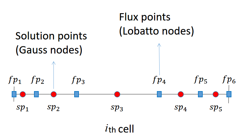
Figure 1: Solution points and flux points in 1D ($K=4$).

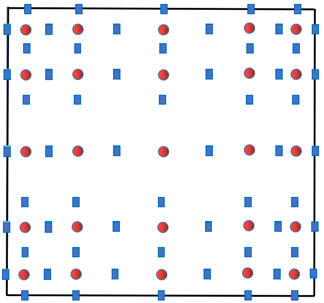
(a) CPR5 cells

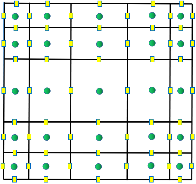
(b) C5NNW5 subcells

Figure 2: Solution points and flux points for CPR5 cells and C5NNW5 subcells ($K=4$), where red circle nodes and square blue nodes in Figure (a) denote solution points and flux points for CPR5, while green circle nodes and yellow square nodes in Figure (b) denote solution points and flux points for C5NNW5.

3 Novel subcell schemes

This section is devoted to develop novel shock capturing schemes based on Legendre-Gauss (LG) solution points, which will be applied in subcell limiting for the high-order CPR method. To ensure the subcell limiting being accurate and robust, both high-order and low-order shock capturing schemes are constructed.

3.1 High-order CNNW schemes

For capturing shock effectively, nonlinear interpolations have been used in MUSCL var Leer [43, 44], WCNS Deng and Zhang [35] and WENO Shu [34] schemes to prevent interpolation across discontinuities. Inspired by nonlinear interpolation in WCNS and compact differencing in CPR, we develop new shock capturing schemes by combining nonlinear interpolation with compact flux differencing. The new shock capturing schemes are constructed through discretizing flux derivative by a compact difference operator based on Riemann fluxes within one cell to make scheme compact, and obtaining the left and right variable values used in Riemann fluxes by nonuniform nonlinear weighted (NNW) interpolation from solution points to flux points on computational space. In the following, the new schemes are called compact nonuniform nonlinear weighted schemes (CNNW).

For a one-dimensional element, solution points and flux points of CNNW schemes are located in staggered form, which means each solution point locates between two flux points. In order to combine with a CPR with LG solution points, we takes $\left(K+1\right)$ LG solution points and $\left(K+2\right)$ Legendre-Gauss-Lobatto (LGL) points as flux points, as shown in Fig. 2. In the following, a fifth-order shock capturing scheme is constructed by using a $5$th-order NNW interpolation and a $5$th-order compact flux difference operator.

3.1.1 The fifth-order compact nonuniform nonlinear weighted scheme (C5NNW5)

Nonuniform nonlinear weighted (NNW) interpolation is taken to obtain the left and right flow-field variable values used in Riemann fluxes at flux points. NNW interpolation takes a stencil of several adjacent solution points, as shown in Fig. 3. A $5$th-order NNW interpolation in one-dimensional case for obtaining the right values at the first flux point of the $i$th cell is given in Appendix A. The NNW interpolation procedure is similar as those in WENO and WCNS. It is worth noticing that there are five LG solution points for each cell and the distances between two adjacent solution points are different.

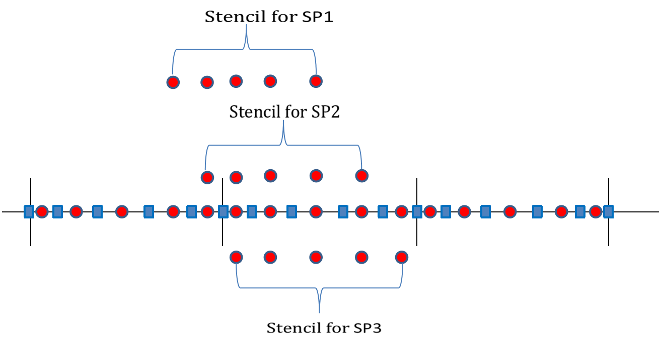
Figure 3: Stencil for high-order interpolation from solution points to flux points

Smoothness indicators used in nonlinear interpolation need to be carefully calculated in the case of nonuniformly spaced solution points. Suppose grid transformation from physical coordinates to computational coordinates is a linear transformation. Then, for the $l$th subcell $[\xi_{fp_{l}},\xi_{fp_{l+1}}]$ we have $x_{\xi}=\frac{\Delta x_{l}}{\Delta\xi_{l}}$ with $\Delta x_{l}=x_{fp_{\left(l+1\right)}}-x_{fp_{l}}$ and $\Delta\xi_{l}=\xi_{fp_{(l+1)}}-\xi_{fp_{l}}$. A smoothness indicator used in WENO schemes [Jiang and Shu [31], Shi et al. [45]] for the $m$th small stencil $S_{i,sp_{l}}^{(m)}$ of the $l$th solution point $sp_{l}$ has the form

$$IS_{m,sp_{l}} =\sum_{\alpha=1}^{2} \int_{x_{fp_{l}}}^{x_{fp_{\left(l+1\right)}}}\left(\Delta x_{l}\right)^{2\alpha-1}\left(\frac{\partial^{\alpha}p_{sp_{l}}^{(m)}}{\partial x^{\alpha}}\right)^{2}dx,$$ (8)

where $p_{sp_{l}}^{(m)}(\xi)$ is a Lagrange interpolation polynomial of degree 2 in the small stencil $S_{i,sp_{l}}^{(m)}$. Then, $\frac{\partial p_{sp_{l}}^{(m)}}{\partial\xi}$ is a linear polynomial and $\frac{\partial^{2}p_{sp_{l}}^{(m)}}{\partial\xi^{2}}$ is a constant. According to $\frac{\partial p_{sp_{l}}^{(m)}}{\partial x}=\frac{\partial p_{sp_{l}}^{(m)}}{\partial\xi}\cdot\frac{1}{x_{\xi}}$, the smoothness indicator in (8) becomes

$$IS_{m,sp_{l}} = \left\{\int_{x_{fp_{l}}}^{x_{fp_{\left(l+1\right)}}}\Delta x_{l}\left(\frac{\partial p_{sp_{l}}^{(m)}}{\partial x}\right)^{2}dx\right\}+\int_{x_{fp_{l}}}^{x_{fp_{(l+1)}}}\left(\Delta x_{l}\right)^{3}\left(\frac{\partial^{2}p_{sp_{l}}^{(m)}}{\partial x^{2}}\right)^{2}dx$$

$$= \left\{\frac{1}{6}\left[\left(\left.\frac{\partial p_{sp_{l}}^{(m)}}{\partial\xi}\right|_{\xi_{fp_{l}}}\right)^{2}+4\left(\left.\frac{\partial p_{sp_{l}}^{(m)}}{\partial\xi}\right|_{\frac{\xi_{fp_{l}}+\xi_{fp_{(l+1)}}}{2}}\right)^{2}+\left(\left.\frac{\partial p_{sp_{l}}^{(m)}}{\partial\xi}\right|_{\xi_{fp_{(l+1)}}}\right)^{2}\right]\left(\Delta\xi_{l}\right)^{2}\right\}$$

$$+\left[\left(\left.\frac{\partial^{2}p_{sp_{l}}^{(m)}}{\partial\xi^{2}}\right|_{sp_{l}}\right)^{2}\left(\Delta\xi_{l}\right)^{4}\right].$$

In this paper, to reduce computation we approximate the term$\int_{x_{fp_{l}}}^{x_{fp_{\left(l+1\right)}}}\Delta x_{l}\left(\frac{\partial p_{sp_{l}}^{(m)}}{\partial x}\right)^{2}dx$ by $\left(\left.\frac{\partial p_{sp_{l}}^{(m)}}{\partial\xi}\right|_{sp_{l}}\right)^{2}\left(\Delta\xi_{l}\right)^{2}$ and obtain the following new simple smoothness indicator:

$$IS_{m,sp_{l}}^{new} = \left(\left.\frac{\partial p_{sp_{l}}^{(m)}}{\partial\xi}\right|_{sp_{l}}\right)^{2}\left(\Delta\xi_{l}\right)^{2}+\left(\left.\frac{\partial^{2}p_{sp_{l}}^{(m)}}{\partial\xi^{2}}\right|_{sp_{l}}\right)^{2}\left(\Delta\xi_{l}\right)^{4}.$$ (9)

After the left and right values at six flux points are obtained by 5th-order NNW interpolation, a $5$th-order compact flux difference operator is used to discretize the flux derivative. Lagrange polynomial based on flux points is

$$\widetilde{F}(\xi)=\sum_{l=1}^{6}\overline{F}_{i,fp_{l}}L_{l}(\xi),$$ (10)

where $\overline{F}_{i,fp_{l}}$ is Riemann flux at LGL flux points $\overline{F}_{i,fp_{l}}(u_{i,fp_{l}}^{L},u_{i,fp_{l}}^{R})$. Here $u_{i,fp_{l}}^{L}$ and $u_{i,fp_{l}}^{R}$ are obtained by the $5$th-order NNW interpolation. Then, the 5th-order compact flux difference operator is obtained by calculating the first-order derivative of the Lagrange polynomial (10) at solution points,

$$\frac{\partial\widetilde{F}}{\partial\xi}|_{i,sp_{m}}=\sum_{l=1}^{6}a_{m,l}\overline{F}_{i,fp_{l}}.$$

The difference between high-order CNNW and high-orde CPR is that CNNW uses nonlinear interpolation based on solution points of the cell and its neighbor cells, uses Riemann fluxes for each flux points, and does not use correction function.

3.2 Low-order CNNW schemes

3.2.1 C2NNW5

A low-order shock capturing scheme with high resolution is constructed by taking 5th-order NNW interpolation proposed in subsection 3.1.1 and Appendix A with following 2nd-order finite difference operator (C2NNW5)

$$\frac{\partial\widetilde{F}}{\partial\xi}|_{i,sp_{l}}=\frac{\overline{F}_{i,fp_{(l+1)}}-\overline{F}_{i,fp_{l}}}{\Delta\xi_{l}},\quad l=1,2,\cdots,K+1$$ (11)

where $sp_{l}$ are LG solution points, $fp_{l}$ are flux points and $\Delta\xi_{l}=\xi_{fp_{(l+1)}}-\xi_{fp_{l}}$.

3.2.2 C2NNW2

A low-order shock capturing scheme with good robustness is constructed by taking a 2nd-order nonlinear weighted interpolation (NNW2) with the 2nd-order finite differential operator in (11) (C2NNW2). The NNW2 interpolation based on a stencil of three adjacent nonuniformly spaced solution points is constructed by using inverse distance weighted interpolation Frink [46] to obtain values at flux points and then using Birth limiter Birth and Jespersen [47] to limit linear reconstruction, as shown in Fig. 4. Details of the NNW2 interpolation are given in Appendix E.

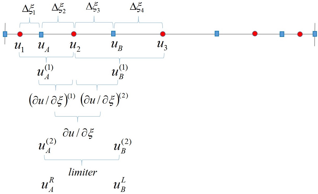
Figure 4: Stencil for NNW2 interpolation from solution points to flux points

3.3 Comparison of interpolation methods and difference operators in CNNW and CPR

Stencils of interpolation and difference operator for CPR5, C5NNW5, C2NNW5, C2NNW2 in solving 1D conservation law are shown in Table 1. For comparison, the fifth-order weighted compact nonlinear scheme (WCNS5) in Deng and Zhang [35] with hybrid cell-edge-node finite difference operator Deng and Zhang [35] is also shown in the Table 1.

Schemes	Interpolation and FD operator	Stencil
CPR5	Lagrange interpolation on Legendre-Gauss SPs:
	$l_{1}u_{i,sp_{1}}+l_{2}u_{i,sp_{2}}+l_{3}u_{i,sp_{3}}+l_{4}u_{i,sp_{4}}+l_{5}u_{i,sp_{5}}$
	Compact FD5 + Correction function:
	$\frac{\partial\widetilde{F}}{\partial\xi}|_{i,sp_{2}}=\sum_{k=1}^{6}a_{k}\widehat{F}_{i,fp_{k}}$+$\delta_{i}$
C5NNW5	NNW5 on Legendre-Gauss SPs:
	$\omega_{1}p_{sp_{2}}^{(1)}+\omega_{2}p_{sp_{2}}^{(2)}+\omega_{3}p_{sp_{2}}^{(3)}$
	Compact FD5:
	$\frac{\partial\widetilde{F}}{\partial\xi}|_{i,sp_{2}}=\sum_{k=1}^{6}a_{k}\overline{F}_{i,fp_{k}}$
C2NNW5	NNW5 on Legendre-Gauss SPs
	$\omega_{1}p_{sp_{2}}^{(1)}+\omega_{2}p_{sp_{2}}^{(2)}+\omega_{3}p_{sp_{2}}^{(3)}$
	FD2:
	$\frac{\partial\widetilde{F}}{\partial\xi}|_{i,sp_{2}}=\frac{1}{\Delta\xi_{2}}(\overline{F}_{i,fp_{3}}-\overline{F}_{i,fp_{2}})$
C2NNW2	NNW2 on Legendre-Gauss SPs:
	$au_{i,sp_{1}}+bu_{i,sp_{2}}+cu_{i,sp_{3}}$
	FD2:
	$\frac{\partial\widetilde{F}}{\partial\xi}|_{i,sp_{2}}=\frac{1}{\Delta\xi_{2}}(\overline{F}_{i,fp_{3}}-\overline{F}_{i,fp_{2}})$
WCNS5	WCNS interpolation on uniformly-spaced SPs:
	$\hat{\omega}_{1}\hat{p}_{sp2}^{(1)}+\hat{\omega}_{2}\hat{p}_{sp2}^{(2)}+\hat{\omega}_{3}\hat{p}_{sp2}^{(3)}$
	Hybrid FD6:
	$\begin{array}[]{ccc}\frac{\partial\widetilde{F}}{\partial\xi}|_{sp2}=&b_{1}(\overline{F}_{i,fp3}-\overline{F}_{i,fp2})\\ &+b_{2}(F_{i,sp3}-F_{i,sp1})&+b_{3}(F_{i,sp4}-F_{i-1,sp5})\end{array}$

Table 1: Stencil of interpolation and FD operators for different schemes at the 2nd solution point of a cell.

4 A priori subcell CNNW limiting approach for CPR method

In this section, a priori subcell limiting approach based on the proposed CNNW schemes is developed for the fifth-order CPR scheme (CPR5) with five Legendre-Gauss solution points presented in Subsection 2.1. Firstly, troubled cell indicators are used to detect troubled cells which may have discontinuities. Then, the troubled cells are decomposed into subcells and computed by the CNNW schemes while other cells are computed by the CPR scheme.

4.1 Troubled cell indicator

In order to find troubled cells, we takes the indicator proposed in Hennemann et al. [30], which follow ideas presented by Persson and Peraire Persson and Peraire [11] and consider the rate of the highest mode to the overall modal energy. Firstly, the representation of the quantity $\epsilon=\rho p$ with Lagrange interpolation polynomials of degree $N$ is transformed to a modal representation with Legendre interpolation polynomials. Secondly, the maximum of proportion of the highest modes and proportion of the second highest mode to the total energy of the Legendre interpolation polynomial is calculated as

$$EI = max\left(\frac{m_{N}^{2}}{\sum_{j=0}^{N}m_{j}^{2}},\frac{m_{N-1}^{2}}{\sum_{j=0}^{N-1}m_{j}^{2}}\right),$$ (12)

where $\{m_{j}|j=0,1,\cdots,N\}$ are the modal coefficients.

In this paper, to consider the jump in cell interfaces, $EI$ is calculated by a higher degree polynomial based on the “extended” stencil consisting of five solution points in the cell and two end points at cell interfaces. Thus, for the $5$th-order CPR, the indicator of the $i$th cell is calculated based on the stencil with seven points $\{\epsilon_{L},\epsilon_{i,1},\epsilon_{i,2},\epsilon_{i,3},\epsilon_{i,4},\epsilon_{i,5},\epsilon_{R}\}$, where $\epsilon_{i,1},\epsilon_{i,2},\epsilon_{i,3},\epsilon_{i,4},\epsilon_{i,5}$ are the quantity $\epsilon=\rho p$ at five solution points, $\epsilon_{L}=aver(\epsilon_{i-1,5},\epsilon_{i,1})$ and $\epsilon_{R}=aver(\epsilon_{i,5},\epsilon_{i+1,1})$ are Roe average values at cell interfaces. Here $aver(\epsilon_{1},\epsilon_{2})=aver(\rho_{1},\rho_{2})\cdot aver(p_{1},p_{2})$ and $aver(\cdot,\cdot)$ is the Roe average function.

We take a threshold value

$$T(N)=a\cdot 10^{-b(N+1)^{1/4}}.$$ (13)

The parameter $b$ is predetermined as $1.8$, which is the same as those in Hennemann et al. [30].

It is worth noticing that for CPR5 with $K=4$ we take $N=K+2=6$ in (12) and (13). In this paper, we set the threshold value in the MDHE indicator (13) to be

$$c(a) = a\cdot 10^{-1.8(6+1)^{1/4}}.$$ (14)

If $EI\geq c(a)$, the element is denoted as a troubled cell. Thus, $c(a)$ control the size of CNNW area.

The indicator based on the rate of the highest mode Persson and Peraire [11] is usually called highest modal decay (MDH) indicator. For simplicity, we denote the highest modal decay indicator based on the “extended” stencil as MDHE indicator in this paper.

4.2 Subcell limiting based on CNNW

After troubled cell detection, the troubled cells are decomposed into subcells and solved by CNNW, as shown in Fig. 5, while other cells are computed by CPR. Thus, a CPR scheme based on subcell CNNW limiting (abbr. CPR-CNNW) is a hybrid scheme. Subcell schemes in troubled cells are chosen according to the magnitude of the MDHE indicator $EI$ in (12) on the extended stencil of $N=K+2$ nodes. To ensure CPR-CNNW having high-resolution and having good robustness in shock capturing, a $p$-adaptive limiting procedure is suggested by using both high-order accurate shock capturing schemes (C5NNW5) and low-order robust shock capturing schemes (C2NNW5 and C2NNW2) to accomplish transition from smooth region to discontinuous region, as shown in Fig. 6.

We define the partition vector $\mathbf{dv}=(S_{1},S_{2},S_{3})$ with three parameters $S_{1}$, $S_{2}$ and $S_{3}$ controlling region division, as shown in Fig. 6. Then, the hybrid CPR-CNNW scheme (abbr. HCCS) can be expressed as

$$\mathrm{HCCS}=\begin{cases}\mathrm{CPR5},&0\leq EI\leq S_{1},\\ \mathrm{C5NNW5},&S_{1}<EI\leq S_{2},\\ \mathrm{C2NNW5},&S_{2}<EI\leq S_{3},\\ \mathrm{C2NNW2},&S_{3}<EI\leq 1.\end{cases}$$ (15)

The hybrid CPR-CNNW scheme is also denoted by $\mathrm{HCCS}(d_{1},d_{2},d_{3},d_{4})$ with $d_{1},d_{2},d_{3},d_{4}$ marking status of CPR, C5NNW5, C2NNW5, C2NNW2 correspondingly. Here $d_{i}=1$ means that the corresponding scheme is contained by the hybrid scheme, otherwise not included. The values of $d_{1},d_{2},d_{3},d_{4}$ are determined by the relationship between the three parameters $S_{1},S_{2},S_{3}$. Thus, by controlling the vector $\mathbf{dv}$, the CPR-CNNW scheme (15) can contain some of the four schemes.

In this paper, we will mainly test a CPR-CNNW scheme with $p$-adaption ($\mathrm{HCCS}(1,1,1,1)$) which contains all of the four schemes and a CPR-CNNW scheme without $p$-adaption ($\mathrm{HCCS}(1,0,0,1)$) which only contains CPR and C2NNW2, as shown in Table 2.

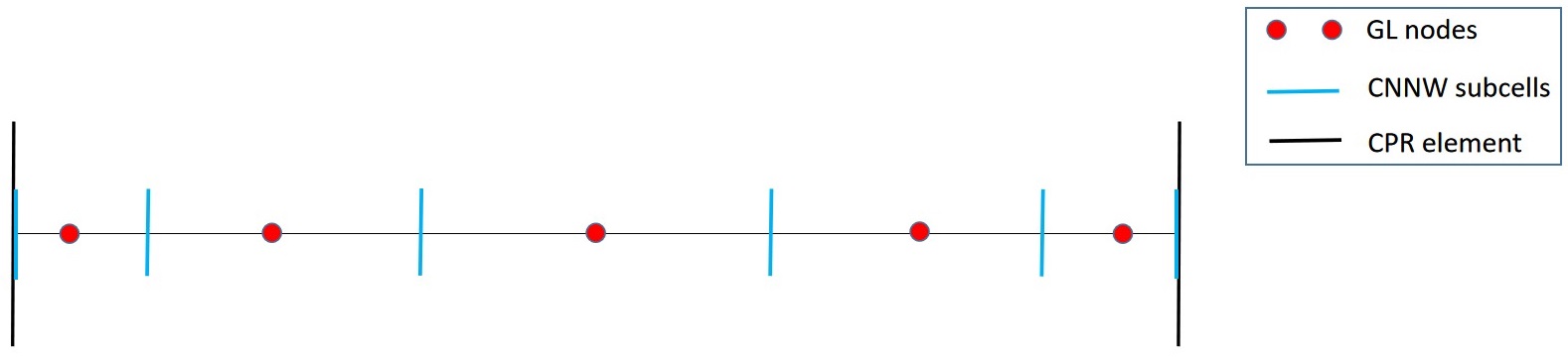
Figure 5: A fifth-order CPR element with CNNW subcells

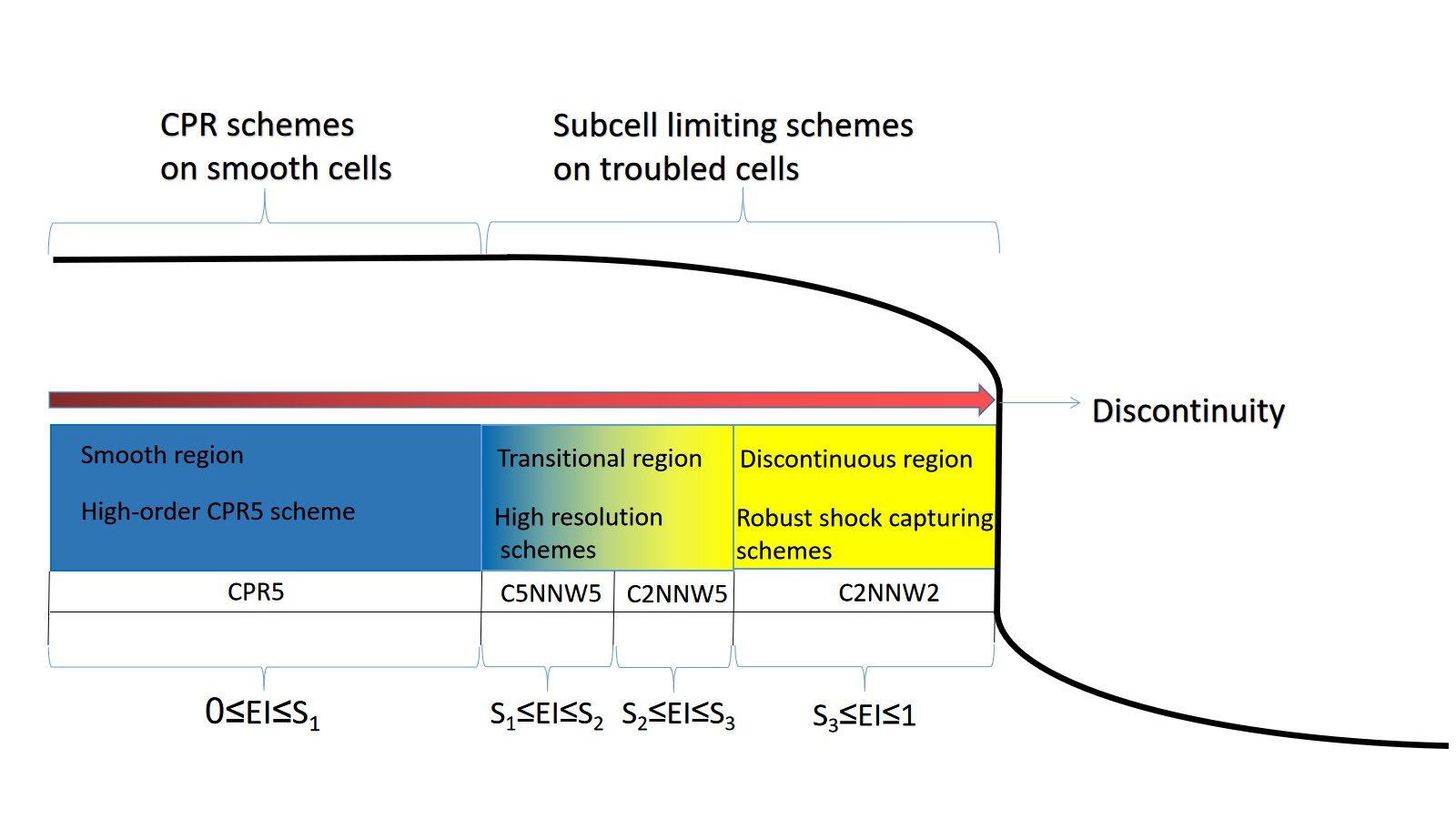
Figure 6: Subcell limiting of CPR-CNNW

Schemes	$\mathrm{HCCS}(d_{1},d_{2},d_{3},d_{4})$	$dv=(S1,S2,S3)$	containing schemes
CPR-CNNW with $p$-adaption	$\mathrm{HCCS}(1,1,1,1)$	0<S1<S2<S3<1	CPR5,C5NNW5,C2NNW5,C2NNW2
CPR-CNNW without $p$-adaption	$\mathrm{HCCS}(1,0,0,1)$	0<S1=S2=S3<1	CPR5,C2NNW2

Table 2: Two CPR-CNNW schemes.

4.3 Interface treatment

CNNW has the same solution points as CPR, which makes the CPR based on subcell CNNW limiting approach have some merits. Firstly, there is no data exchange between solution points of different schemes and thus the proposed hybrid scheme can take less computations. Secondly, extra state values required in interpolation method on troubled cells are taken from neighboring cells directly, and thus there is no need to add ghost cells for exchanging the state values.

The only thing needed to do in interface treatment is calculation of Riemann fluxes at the interface of different schemes. The Riemann fluxes at the interface of scheme A and scheme B are calculated based on the left and right values interpolated from scheme A and scheme B, correspondingly. For example, Riemann fluxes at the interface of CPR and C5NNW5 are computed based on one side from CPR cell and the other from C5NNW5.

5 Theoretical analysis on spectral properties and conservation

5.1 Spectral properties of high-order CNNW and CPR

Finite difference schemes usually obtain the spectrum by Fourier method while DG-type method which locates several solution points in one cell usually calculate the spectrum based on local discrete matrices. To make fair comparisons, the eigenvalues of spatial discretization matrix of different schemes are calculated by the same method on local discrete matrices. We analyze the spectrum by local discrete matrices and prove that all eigenvalues comes from the same function and each scheme has a unique spectrum curve.

Suppose the computational domain is decomposed to $M$ cells. The semi-discretization form of one-dimensional linear advection equation $u_{t}+u_{x}=0$ with periodic boundary condition can be written as the first form:

$$\frac{\partial}{\partial t}\mathbf{U}=\frac{1}{\Delta x}E\mathbf{U}$$ (16)

where $\mathbf{U}=(u_{1},u_{2},\cdots,u_{(K+1)M})^{T}$, $\Delta x$ is spatial step and $-\frac{1}{\Delta x}E$ is spatial discretization matrix of first-order derivative. The semi-discretization form can also be written as the second form:

$$\frac{\partial}{\partial t}\left[\begin{array}[]{c}u_{j,1}\\ u_{j,2}\\ \vdots\\ u_{j,K+1}\end{array}\right] =\frac{1}{(K+1)\Delta x} \left(A\left[\begin{array}[]{c}u_{j-1,1}\\ u_{j-1,2}\\ \vdots\\ u_{j-1,K+1}\end{array}\right]+B\left[\begin{array}[]{c}u_{j,1}\\ u_{j,2}\\ \vdots\\ u_{j,K+1}\end{array}\right]+C\left[\begin{array}[]{c}u_{j+1,1}\\ u_{j+1,2}\\ \vdots\\ u_{j,K+1}\end{array}\right]\right)$$ (33)

where $j=1,2,\cdots,M$. Then, the matrix $E$ can be written as

$$E = \frac{1}{K+1}\left[\begin{array}[]{cccccc}B&C&0&0&0&A\\ A&B&C&0&0&0\\ 0&A&B&C&0&0\\ 0&0&A&B&C&0\\ 0&0&0&A&B&C\\ C&0&0&0&A&B\end{array}\right]_{(K+1)M\times(K+1)M},$$ (40)

where $A$, $B$, $C$ are $(K+1)\times(K+1)$ matrix. The matrix $E$ is a block circulant matrix.

In the following Theorem 2.1, we prove that all eigenvalues of the spatial discretization matrix can be obtained by collecting the eigenvalues of local spatial matrices. In addition, all eigenvalues comes from the same function and thus all the eigenvalues are on a unique spectrum curve.

Theorem 2.1 The matrix $E$ in spacial discretization matrix with form (40) has following properties:

(1)All the eigenvalues of $E$ are given by

$$\{x|EX=xX,\,X\in\mathbb{C}^{(K+1)M}\} = \sum_{m=0}^{M-1}\{x|H_{m}Y_{m}=xY_{m},\,Y_{m}\in\mathbb{C}^{K+1}\},$$

where $H_{m}=H(\phi_{m})$, $\phi_{m}=m\frac{2\pi}{M},\,\,m=0,1,2,\cdots,M-1$ and

$$H(\phi) = \left(Ae^{-i\phi}+B+Ce^{i\phi}\right)/(K+1),\,\,\,\,0\leq\phi<2\pi.$$ (41)

In other word, $SH\triangleq Spec\left(E\right)=\left\{Spec\left(H_{0}\right),Spec\left(H_{1}\right),\cdots,Spec\left(H_{M-1}\right)\right\}$.

(2) Suppose $G_{m}=G(\phi_{m})$ with

$$G(\phi) = \left(Ae^{-i\phi(K+1)}+B+Ce^{i\phi(K+1)}\right)/(K+1),\,\,\,\,0\leq\phi<2\pi,$$ (42)

and $Spec\left(G_{m}\right)=\{\lambda^{(l)}(G(\phi_{m}))|l=1,2,\cdots,K+1\}$, $SG\triangleq\left\{Spec\left(G_{0}\right),Spec\left(G_{1}\right),\cdots,Spec\left(G_{M-1}\right)\right\}$, where $\phi_{m}=m\frac{2\pi}{M},\,\,m=0,1,2,\cdots,M-1$. It can be proved that if $mod(M,K+1)\neq 0$ then

$$SG = SH,$$

else

$$SG=\left\{Spec\left(H_{0}\right),Spec\left(H_{(K+1)}\right),Spec\left(H_{2(K+1)}\right),\cdots,Spec\left(H_{L(K+1)}\right)\right\} \subset SH,\,\,\,\,SG\neq SH.$$

(3) It can be proved that the $(K+1)$ eigenvalues of $G_{m}$ are

$$\lambda^{(l)}\left(G_{m}\right) =\lambda^{(l)}\left(\phi_{m}\right)= \lambda^{(1)}\left(\phi_{m}-(l-1)\frac{2\pi}{\left(K+1\right)}\right),\,\,l=1,2,\cdots,K+1,$$

where $\phi_{m}=m\frac{2\pi}{M},\,\,m=0,1,2,\cdots,M-1$. Classify $SG$ as $(K+1)$th groups,

$$SG=\cup_{l=1}^{K+1}Group{}^{(l)}$$

with $Group^{(l)}=\left\{\left.\lambda^{(l)}\left(G_{m}\right)\right|\phi_{m}=m\frac{2\pi}{M},\,\,m=0,1,2,\cdots,M-1\right\}$. If $mod(M,K+1)=0$, then eigenvalues in each group are the same $Group^{(1)}$=$\cdots$=$Group^{(K+1)}$.

(4) $SG$ can be written as

$$SG = \begin{cases}\left\{\left.\lambda^{(1)}(G(\psi_{(K+1)m}))\right|m=0,1,\cdots,M-1\right\},\,\,&if\,\,\,mod(M,K+1)=0,\\ \left\{\left.\lambda^{(1)}(G(\psi_{j}))\right|j=0,1,2\cdots,M(K+1)\right\}&else,\end{cases}$$

which means that all eigenvalues comes from the same function. Here $\psi_{j}=\frac{2\pi j}{M(K+1)}$.

The proof of the Theorem 2.1 is given in Appendix B.

A pure upwind flux $\overline{u}=u^{L}$ is used to compute the common fluxes, where $u^{L}$ is the left value at flux points. An example is given to explain the properties of the eigenvalues of local discrete matrices and the unique spectral curve of a scheme in Appendix C. Comparisons on spectrum of different high-order schemes are given in Appendix D.

Dispersion and dissipation characteristics for fifth-order schemes are shown in Fig. 7, where real part and imaginary part of eigenvalues computed from local matrix $G$ in (42) with $\phi_{m}=m\frac{2\pi}{M},\,\,m=0,1,2,\cdots,M-1$ and $M=40$. We can see that all eigenvalues come from the same function and the eigenvalue curves can coincide with each other after a shift of $\frac{2\pi}{K+1}$, which agrees with the property (3) in Theorem 5.1 under the case $M=40$, $K+1=5$ and $mod(M,K+1)=0$. This translation phenomenon was also found by Moura in Moura et al. [48]. The spectral properties of third-order schemes are given in Appendix D.

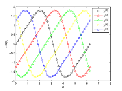
(a) C5NNW5, dispersion

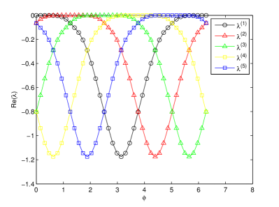
(b) C5NNW5, dissipation

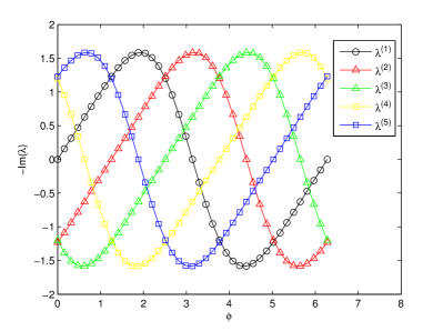
(c) WCNS5, dispersion

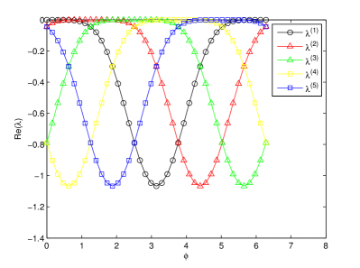
(d) WCNS5, dissipation

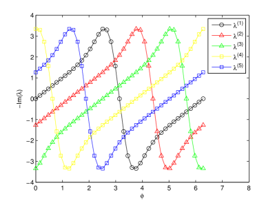
(e) CPR5, dispersion

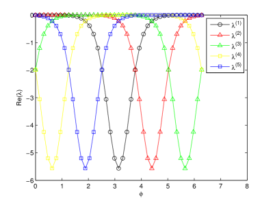
(f) CPR5, dissipation

Figure 7: Comparison of dispersion (left) and dissipation (right) eigencurves for fifth-order schemes, where $\left\{\lambda_{m}^{(l)}\left|\lambda_{m}^{(l)}=\lambda^{(l)}(G(\phi_{m})),l=1,2,\cdots K+1;m=0,1,2,\cdots,M\right.\right\}$, $\phi_{m}=m\frac{2\pi}{M}$, $K=4$ and $M=40$.

Comparisons of different schemes show that the spectral property of the proposed CNNW is closer to WCNS than CPR. Form Fig. 8(a)(c) we can see that C3NNW3 has smaller dispersion errors than WCNS3. For fifth-order schemes, C5NNW5 has smaller dispersion errors than WCNS5 at area $\phi_{0}\leq\phi<\pi$ but bigger dispersion errors for $0\leq\phi<\phi_{0}$, where $\phi_{0}\approx 0.3772$. As for dissipation errors, CNNW has similar errors as WCNS for both of the third-order schemes and fifth-order schemes, which can been seen from Fig. 8(b)(d).

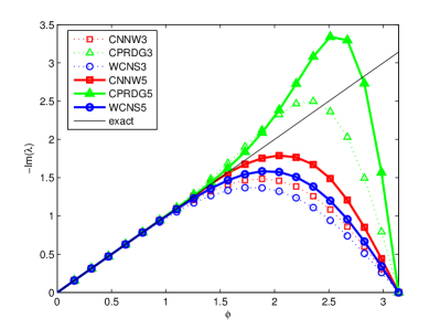
(a) Dispersion

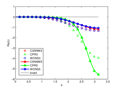
(b) Dissipation

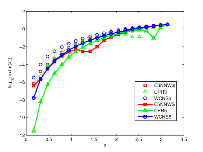
(c) Dispersion errors

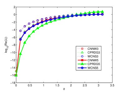
(d) Dissipation errors

Figure 8: comparison of dispersion and dissipation for third-order schemes and fifth-order schemes

5.2 Discrete conservation laws

5.2.1 Discrete conservation laws of high-order CNNW

In order to satisfy one-dimensional conservation law (CL), the following integral conservation law in a cell $[x_{i},x_{i+1}]$ should be satisfied, i.e.,

$$\int_{x_{i}}^{x_{i+1}}\frac{\partial u^{h}}{\partial t}dx+\left(\widetilde{F}(x_{i+1})-\widetilde{F}(x_{i})\right) = 0.$$

For each solution point, CNNW with $\left(K+1\right)$th-order of accuracy reads

$$\frac{\partial u_{i,l}}{\partial t}=-\frac{2}{h}\frac{\partial\widetilde{F}}{\partial\xi}|_{i,l}=-\frac{2}{h}\sum_{j=1}^{K+2}a_{j}\overline{F}_{i,j},\quad l=1,2,\cdots,K+1.$$

Thus, we can obtain

$$\frac{\partial\left(\int_{x_{i}}^{x_{i+1}}u^{h}dx\right)}{\partial t} = \frac{h}{2}\frac{\partial\left(\int_{-1}^{1}u^{h}d\xi\right)}{\partial t}=\frac{h}{2}\frac{\partial\left(\sum_{l=1}^{K+1}2w_{l}u_{i,l}\right)}{\partial t}$$

$$= \frac{h}{2}\sum_{l=1}^{K+1}2w_{l}\left(\frac{\partial u_{i,l}}{\partial t}\right)=\sum_{l=1}^{K+1}2w_{l}\left(-\frac{\partial\widetilde{F}}{\partial\xi}|_{i,l}\right).$$

where $w_{l}$ are the weights in Gaussian quadrature formulas. When $K=4$, we have

$$w_{1}=\frac{322-13\sqrt{70}}{1800},\quad w_{2}=\frac{322+13\sqrt{70}}{1800},\quad w_{3}=\frac{64}{225},\quad w_{4}=w_{2},\quad w_{5}=w_{1}.$$ (44)

Since flux polynomial is the Lagrange polynomial based on Riemann fluxes at $(K+2)$th flux points,

$$\widetilde{F}(\xi)=\sum_{l=1}^{K+2}\overline{F}_{i,fp_{l}}L_{l}(\xi),$$

$\widetilde{F}$ is a $K+1$ degree polynomial. Then, $\frac{\partial\widetilde{F}}{\partial\xi}$ belongs to $P^{K}$. Since the quadrature rule based on $K+1$ points has at least $K$ algebraic accuracy, the rule is exact for degree $K$ polynomial $\left(\frac{\partial\widetilde{F}}{\partial\xi}\right)$. Thus, we have

$$\sum_{l=1}^{K+1}2w_{l}\left(-\frac{\partial\widetilde{F}}{\partial\xi}|_{i,l}\right) = -\int_{-1}^{1}\left(\frac{\partial\widetilde{F}}{\partial\xi}\right)d\xi=-\left(\widetilde{F}(1)-\widetilde{F}(-1)\right)$$

$$= -\left(\overline{F}_{i,fp_{K+2}}-\overline{F}_{i,fp_{1}}\right)=-\left(\overline{F}_{i}(1)-\overline{F}_{i}(-1)\right).$$

According to (5.2.1) and (5.2.1), we obtain following relation

$$\frac{\partial\left(\sum_{l=1}^{K+1}w_{l}u_{i,l}\right)}{\partial t} = -\left(\overline{F}_{i}(1)-\overline{F}_{i}(-1)\right).$$

Therefore, high-order CNNW satisfies discrete conservation laws.

Remark 5.1. Suppose flux derivatives at solutions points are calculated by the Lagrange interpolation polynomial using all flux points in the cell. If a cell has $K+1$ solution points and flux points are less equal to $K+2$, then CNNW satisfies discrete conservation law no matter which kind of solution points and flux points are selected. When $K+1$ Legendre-Gauss solution points are used, then CNNW satisfies discrete conservation law if flux points are less equal to $2K+1$.

For two-dimensional case, we have

$$\frac{\partial u_{i,j,l,m}}{\partial t} = -\frac{4}{h^{2}}\left(\frac{\partial\widetilde{F}}{\partial\xi}|_{i,j,l,m}+\frac{\partial\widetilde{G}}{\partial\eta}|_{i,j,l,m}\right)$$

$$= -\frac{4}{h^{2}}\left(\sum_{k=1}^{K+2}c_{l,k}\overline{F}_{i,j,fp_{k},m}+\sum_{k=1}^{K+2}c_{m,k}\overline{G}_{i,j,l,fp_{k}}\right).$$

Then, it can be easily proved that the discrete conservation law is

$$\frac{\partial\sum_{l=1}^{K+1}\sum_{m=1}^{K+1}w_{l}w_{m}u_{i,j,l,m}}{\partial t}$$

$$= -\frac{4}{h^{2}}\left[\sum_{m=1}^{K+1}w_{m}\left(\sum_{l=1}^{K+1}w_{l}\frac{\partial\widetilde{F}}{\partial\xi}|_{i,j,l,m}\right)+\sum_{l=1}^{K+1}w_{l}\left(\sum_{m=1}^{K+1}w_{m}\frac{\partial\widetilde{G}}{\partial\eta}|_{i,j,l,m}\right)\right]$$

$$= -\frac{4}{h^{2}}\left[\sum_{m=1}^{K+1}w_{m}\left(\overline{F}(1,\eta_{m})-\overline{F}(-1,\eta_{m})\right)+\sum_{l=1}^{K+1}w_{l}\left(\overline{G}(\xi_{l},1)-\overline{G}(\xi_{l},-1)\right)\right].$$

5.2.2 Discrete conservation law of C2NNW5 and C2NNW2

For each solution point, we have

$$\frac{\partial u_{i,sp_{l}}}{\partial t}=-\frac{2}{h}\frac{\partial\widetilde{F}}{\partial\xi}|_{i,sp_{l}}=-\frac{2}{h}\frac{\overline{F}_{i,fp_{(l+1)}}-\overline{F}_{i,fp_{l}}}{\Delta\xi_{l}}.$$

Then, we can obtain

$$\frac{\partial\left(\int_{x_{i}}^{x_{i+1}}u^{h}dx\right)}{\partial t} = \frac{h}{2}\frac{\partial\left(\int_{-1}^{1}u^{h}d\xi\right)}{\partial t}=\frac{h}{2}\frac{\partial\left(\sum_{m=1}^{K+1}\int_{\xi_{i,fp_{l}}}^{\xi_{i,fp_{(l+1)}}}u^{h}d\xi\right)}{\partial t}$$

$$= \frac{h}{2}\frac{\partial\left(\sum_{l=1}^{K+1}u_{i,sp_{l}}\Delta\xi_{l}\right)}{\partial t}=\frac{h}{2}\left(\sum_{l=1}^{K+1}\Delta\xi_{l}\frac{\partial u_{i,sp_{l}}}{\partial t}\right)$$

$$= \frac{h}{2}\left(\sum_{l=1}^{K+1}\Delta\xi_{l}\left(-\frac{2}{h}\frac{\overline{F}_{i,fp_{(l+1)}}-\overline{F}_{i,fp_{l}}}{\Delta\xi_{l}}\right)\right)=\sum_{l=1}^{K+1}-\left(\overline{F}_{i,fp_{(l+1)}}-\overline{F}_{i,fp_{l}}\right)$$

$$= -\left(\overline{F}_{i,fp_{(K+2)}}-\overline{F}_{i,fp_{1}}\right)=-\left(\overline{F}_{i}(1)-\overline{F}_{i}(-1)\right).$$

Therefore, C2NNW5 and C2NNW2 satisfy following discrete conservation law

$$\frac{\partial\left(\sum_{l=1}^{K+1}u_{i,sp_{l}}\Delta\xi_{l}\right)}{\partial t}=-\left(\overline{F}_{i}(1)-\overline{F}_{i}(-1)\right).$$

For two-dimensional case, it can be easily proved that the discrete conservation law is

$$\frac{\partial\sum_{l=1}^{K+1}\sum_{m=1}^{K+1}\Delta\xi_{l}\Delta\eta_{m}u_{i,j,l,m}}{\partial t}$$ (47)

$$= -\frac{4}{h^{2}}\left[\sum_{m=1}^{K+1}\Delta\eta_{m}\left(\sum_{l=1}^{K+1}\Delta\xi_{l}\frac{\partial\widetilde{F}}{\partial\xi}|_{i,j,l,m}\right)+\sum_{l=1}^{K+1}\Delta\xi_{l}\left(\sum_{m=1}^{K+1}\Delta\eta_{m}\frac{\partial\widetilde{G}}{\partial\eta}|_{i,j,l,m}\right)\right]$$

$$= -\frac{4}{h^{2}}\left[\sum_{m=1}^{K+1}\Delta\eta_{m}\left(\overline{F}(1,\eta_{m})-\overline{F}(-1,\eta_{m})\right)+\sum_{l=1}^{K+1}\Delta\xi_{l}\left(\overline{G}(\xi_{l},1)-\overline{G}(\xi_{l},-1)\right)\right].$$

Therefore, the discrete conservation law holds for both C2NNW5 and C2NNW2.

5.2.3 Discrete conservation law of the CPR-CNNW scheme

CPR and C5NNW5 has discrete conservation law in (5.2.1), while the discrete conservation law for C2NNW5 and C2NNW2 has the form in (47). To make the CPR-CNNW scheme satisfying discrete conservation law, it is necessary to have the same form of discrete conservation laws for different schemes. Thus, we choose flux points $\xi_{fp_{m}}=-1+\sum_{l=1}^{m-1}w_{l}$ for C2NNW5 and C2NNW2. Here $w_{l}$ are the Legendre-Gauss weights in (44). Then $\Delta\xi_{l}=w_{l}$ and $\Delta\eta_{m}=w_{m}$, the discrete conservation law in (47) of C2NNW5 and C2NNW2 becomes the same as the form (5.2.1). Then, the C2NNW5 and C2NNW2 have the same form of discrete conservation law with that of C5NNW5, which means that the Riemann fluxes at cell interfaces will be eliminated during total summation. Therefore, the hybrid schemes also satisfy discrete conservation law. The splitting of a CPR element into subcells based on Gauss weights is similar as that done by Sonntag et al. Sonntag and Munz [28] for DG method with Gauss solution points and by Hennemann et al. Hennemann et al. [30] for DG method with Legendre-Gauss-Lobatto solution points.

6 Numerical investigation

In this section, seven test cases are adopted for both one-dimensional and two-dimensional hyperbolic conservation laws to illustrate the following properties of the CPR-CNNW schemes: (1) high resolution; (2) good shock capturing robustness; (3) satisfying discrete conservation. The test cases adopted and the properties studied in these test cases have been summarized in Tab. 3.

Sections Equations Test cases Purpose 6.1 1D advection Advection of smooth wave Order of accuracy 6.2 1D Euler Shock tube problems Shock capturing (Numerical oscillations) 6.3 1D Euler Shu-Osher problem Resolution, Scheme adaption strategy Influence of indicating on resolution Shock capturing (Comparison with others) 6.4 2D Euler Isentropic vortex problem Order of accuracy, influence of indicating on accuracy Time evolution of errors, Discrete conservation, 6.5 2D Euler Riemann problem Resolution, Influence of indicating on resolution Shock capturing (Quantitative study) 6.6 2D Euler Double Mach reflection Resolution, Shock capturing (Strong shocks) 6.7 2D Euler Shock vortex interaction Resolution, Shock capturing

Table 3: Summary of test cases

Unless otherwise specified, $a=0.5$ is used and then $c_{0}=c(0.5)=0.5\cdot 10^{-1.8(6+1)^{1/4}}\approx 5.90\times 10^{-4}$ is applied to control the size of CNNW area. Partition vector $\mathbf{dv}=(c_{0},0.05,0.1)$ and $\mathbf{dv}=(c_{0},c_{0},c_{0})$ in (15) will be applied to obtain HCCS(1,1,1,1) and HCCS(1,0,0,1) respectively. The Z-weights in Formula (53) in Appendix A with $\varepsilon=10^{-10}$ is used for computing nonlinear weights in the NNW procedure. By default, in shock capturing test cases, characteristic variables are applied in the NNW interpolations. The Lax-Friedrichs flux is adopted to compute common fluxes. The explicit third-order TVD Runge-Kutta scheme is used for time integration.

6.1 1D linear advection equation with a smooth solution

An accuracy test is conducted based on the one-dimensional (1D) linear advection equation

$$u_{t}+u_{x} = 0.$$

The problem is solved in a spatial domain of $[-3,3]$ with initial condition $u(x,0)=sin\left(\frac{\pi x}{3}\right)$ till time $T=3$. The $L_{2}$ and $L_{\infty}$ errors, as well as the numerical order of accuracy, are summarized in Tabs. 4 and 5 for the fifth-order schemes and in Tab. 6 for the second-order schemes. As expected, C5NNW5 reaches fifth-order of accuracy. In addition, C5NNW5 has smaller numerical errors than the fifth-order CPR-g2 scheme with Legendre-Gauss-Lobatto solution points and $g_{2}$ correction function (see references Huynh [7], Zhu et al. [37] for details), while C5NNW5 has bigger errors than WCNS5 and CPR5. For the second-order schemes, C2NNW5 has smaller errors than C2NNW2 for both linear schemes and nonlinear schemes.

$Norm$	DoFs	C5NNW5		WCNS5		CPR-g2		CPR5
		error	order	error	order	error	order	error	order
$L_{\infty}$	$15$	9.04E-04	-	6.55E-04	-	5.28E-03	-	5.72E-04	-
	$30$	2.74E-05	5.04	2.09E-05	4.97	1.77E-04	4.90	1.28E-05	5.48
	$60$	8.10E-07	5.08	6.58E-07	4.99	5.93E-06	4.90	4.38E-07	4.87
	$120$	2.54E-08	5.00	2.06E-08	5.00	1.84E-07	5.01	1.41E-08	4.95
	$240$	7.97E-10	4.99	6.44E-10	5.00	5.72E-09	5.01	4.55E-10	4.96
$L_{2}$	$15$	5.90E-04	-	4.64E-04	-	1.94E-03	-	3.18E-04	-
	$30$	1.80E-05	5.03	1.48E-05	4.97	6.43E-05	4.91	9.48E-06	5.07
	$60$	5.63E-07	5.00	4.65E-07	4.99	2.03E-06	4.99	2.98E-07	4.99
	$120$	1.77E-08	4.99	1.46E-08	4.99	6.29E-08	5.01	9.23E-09	5.01
	$240$	5.54E-10	5.00	4.55E-10	5.00	1.95E-09	5.01	2.85E-10	5.02

Table 4: Accuracy test results of the high-order linear schemes in solving 1D linear equation. Here “linear” indicates that the optimal linear weights are adopted for the NNW interpolation procedure.

$Norm$	DoFs	C5NNW5		WCNS5
		error	order	error	order
$L_{\infty}$	$15$	3.94E-02	-	5.67E-03	-
	$30$	4.68E-04	6.40	2.05E-04	4.79
	$60$	9.53E-06	5.62	6.59E-06	4.96
	$120$	2.39E-07	5.32	2.04E-07	5.01
	$240$	7.58E-09	4.98	6.03E-09	5.08
$L_{2}$	$15$	1.98E-02	-	3.73E-03	-
	$30$	2.83E-04	6.13	1.23E-04	4.92
	$60$	5.16E-06	5.78	3.74E-06	5.04
	$120$	1.52E-07	5.09	1.14E-07	5.04
	$240$	4.76E-09	5.00	3.53E-09	5.01

Table 5: Accuracy test results of the high-order nonlinear schemes in solving 1D linear equation.

Norm	N	linear schemes				nonlinear schemes
		C2NNW5		C2NNW2		C2NNW5		C2NNW2
		error	order	error	order	error	order	error	order
$L_{\infty}$	$15$	3.88E-02	-	7.15E-02	-	4.25E-02	-	1.38E-01	-
	$30$	8.61E-03	2.17	1.61E-02	2.15	9.29E-03	2.19	4.33E-02	1.68
	$60$	2.17E-03	1.99	3.95E-03	2.02	2.22E-03	2.07	1.49E-02	1.53
	$120$	5.35E-04	2.02	9.57E-04	2.05	5.35E-04	2.05	6.17E-03	1.28
	$240$	1.33E-04	2.01	2.38E-04	2.01	1.33E-04	2.01	2.57E-03	1.26
$L_{2}$	$15$	2.55E-02	-	4.73E-02	-	2.85E-02	-	6.20E-02	-
	$30$	6.00E-03	2.09	1.10E-02	2.10	6.42E-03	2.15	1.97E-02	1.65
	$60$	1.47E-03	2.03	2.67E-03	2.04	1.55E-03	2.05	6.30E-03	1.65
	$120$	3.66E-04	2.01	6.61E-04	2.01	3.82E-04	2.02	1.85E-03	1.77
	$240$	9.13E-05	2.00	1.65E-04	2.00	9.31E-05	2.04	5.67E-04	1.71

Table 6: Accuracy test results of the second-order schemes in solving 1D linear equation.

6.2 1D Shock tube problems

The shock tube problems are solved to test the shock-capturing capability of the CNNW and CPR-CNNW. The Sod problem with initial conditions

$$\left(\rho,u,p\right)=\begin{cases}\left(1,0,1\right),&0\leq x<0.5,\\ (0.125,0,0.1),&0.5\leq x<1,\end{cases}$$

is solved till $t=0.2$ with $40$ cells and $DoFs=200$. In addition, the Lax problem with initial conditions

$$\left(\rho,u,p\right)=\begin{cases}\left(0.445,0.698,3.528\right),&0\leq x<0.5,\\ (0.5,0,0.571),&0.5\leq x<1,\end{cases}$$

is solved till $t=0.1$ with $100$ cells and $DoFs=500$.

Firstly, the CNNW schemes are used to solve these problems. The computed density distributions are shown in Fig. 9. In the Sod problem, there is no obvious numerical oscillation for simulations with C5NNW5, C2NNW5 and C2NNW2. Moreover, the C5NNW5 acquires a similar result as that of the WCNS5. For the second-order schemes, C2NNW5 results in sharper discontinuities than the C2NNW2. For the Lax problem with stronger discontinuities, the results of the C5NNW5, C2NNW5 and C2NNW2 have small oscillations near the location $x=0.74$ while there is no obvious oscillations for the result of the WCNS.

Secondly, CPR-CNNW schemes are applied to solve these problems. The results are shown in Fig. 10. We can see that both HCCS(1,1,1,1) and HCCS(1,0,0,1) can capture shock robustly. In addition, there are only 1-2 troubled cells near each discontinuity. Symbols are also given to highlight the values at all solution points. For both HCCS(1,1,1,1) and HCCS(1,0,0,1), the shock thickness is close to the element length and 6 solution points can nearly recover the discontinuity, which indicates that the present limiting method has a subcell resolution.

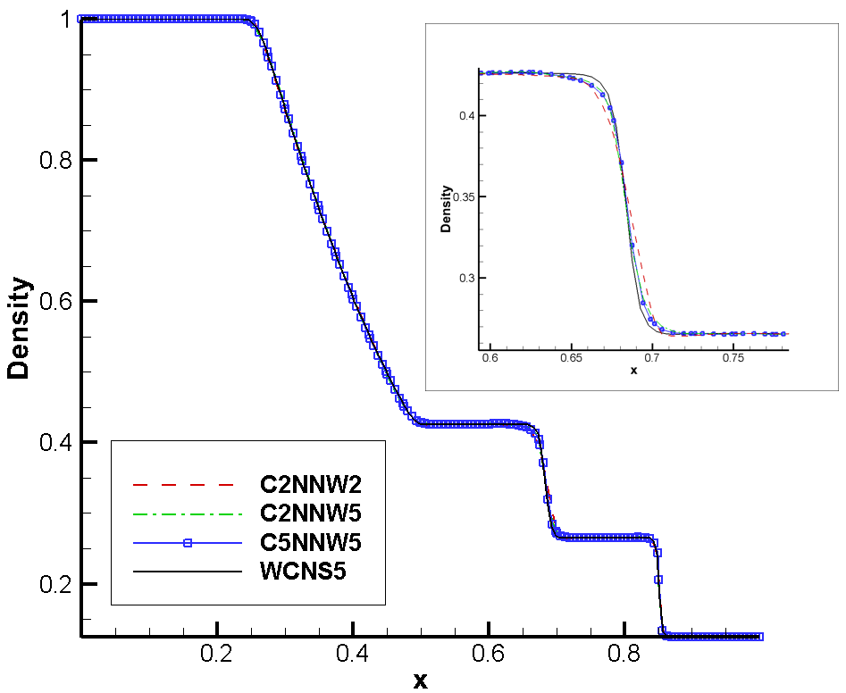
(a) Sod problem, $DOFs=200$

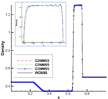
(b) Lax problem, $DOFs=500$

Figure 9: Density distribution of single schemes in solving 1D shock tube problems.

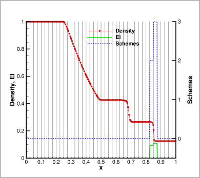
(a) Sod problem, HCCS(1,1,1,1), $DOFs=200$

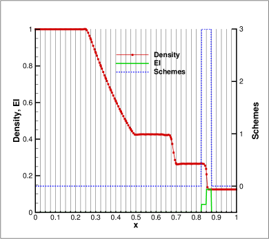
(b) Sod problem, HCCS(1,0,0,1), $DOFs=200$

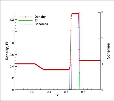
(c) Lax problem, HCCS(1,1,1,1), $DOFs=500$

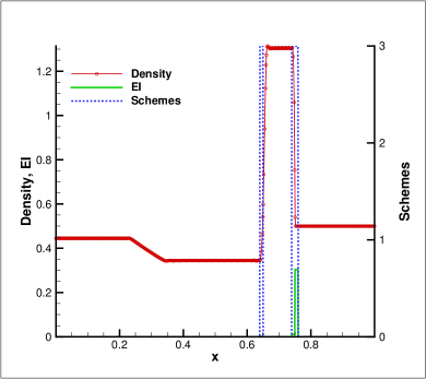
(d) Lax problem, HCCS(1,0,0,1), $DOFs=500$

Figure 10: Hybrid schemes HCCS(1,1,1,1) and HCCS(1,0,0,1) in solving 1D shock tube problems. Here schemes 0, 1, 2, 3 represent CPR, C5NNW5, C2NNW5 and C2NNW2, correspondingly.

6.3 Shu-Osher problem

The Shu-Osher problem with initial conditions

$$\left(\rho,u,p\right)=\begin{cases}\left(3.857143,2.629369,10.333333\right),&-5\leq x<-4,\\ (1.0+0.2sin(5x),0,1.0),&-4\leq x<5,\end{cases}$$

is solved till $t=1.8$ with $DoFs=400$.

Firstly, the CNNW schemes are used to solve the problem and are compared with WCNS. The computed density distributions are shown in Fig. 11. C5NNW5, C2NNW5 and C2NNW2 can capture shocks without obvious oscillations. In addition, C5NNW5 has the highest resolution, which is similar as WCNS5. On the contrary, the C2NNW2 has lowest resolution.

Secondly, CPR-CNNW schemes are tested in this problem. HCCS(1,1,1,1) with $\mathbf{dv}=(c(a),0.05,0.1)$ and HCCS(1,0,0,1) with $\mathbf{dv}=(c(a),c(a),c(a))$ under different $a$ are applied to solve this problem. We consider three cases $a=0.5$, $a=0.05$ and $a=0.005$. From Fig. 12, we can see that both HCCS(1,1,1,1) and HCCS(1,0,0,1) can capture shocks very well without obvious oscillations. The numbers of troubled cells of HCCS(1,1,1,1) at $t=1.8$ are 2, 8, 19 for $a=0.5$, $a=0.05$ and $a=0.005$, correspondingly and the numbers of troubled cells of HCCS(1,0,0,1) are 3, 7, 19, correspondingly. Comparing Fig. 12(c) and (d), we can see that HCCS(1,1,1,1) has much higher resolution than HCCS(1,0,0,1). HCCS(1,1,1,1) can still obtain similar resolution during increasing the number of troubled cells (by increasing $a$) while the resolution of HCCS(1,0,0,1) decrease dramatically. Thus, indicating wrongly will affect the resolution of CPR with second-order CNNW limiting (HCCS(1,0,0,1)) since second-order CNNW scheme may be used in smooth region. However it has less influences on the resolution of CPR with p-adaptive CNNW limiting (HCCS(1,1,1,1)) since just few troubled cells in shocks are computed by second-order schemes and most troubled cells will be computed by C5NNW5 which also have high-order of accuracy in smooth region. This results indicate that it is better to include the high-order scheme C5NNW5 or the high resolution scheme C2NNW5 in subcell limiting to keep high resolution.

Thirdly, the CPR-CNNW schemes are compared with other four shock capturing FE schemes. The following four results are compared: (1) the result computed by DG-$P4$ with artificial viscosity, the MDH model and DoFs=600 in Discacciati et al. [12]; (2) the result of DG-$P3$ with simple WENO limiter Zhong and Shu [9], Zhu et al. [18], Du et al. [19] under DoFs=400 from Fig. 1(a) in Li et al. [20]; (3) the result of DG-$P5$ with $p$-weighted limiter under DoFs=600 in Fig. 1(d) in Li et al. [20]; (4) the result of DG-$P4$ with subcell shock limiting based on LGL nodes under DoFs=640 in Fig. 5(c) in Hennemann et al. [30]. as Comparisons are shown in Fig. 13. We can see that HCCS(1,1,1,1) can obtain similar results in capturing the high-frequent waves with fewer DoFs (DoFs=400). In addition, both the simple WENO limiter and the $p$-weighted limiter lead to obvious deviations in wave phase in Fig. 13(b) and Fig. 13(c). The simple WENO limiter has obvious oscillations near $x=-2$ as shown in Fig. 13(b) while the $p$-weighted limiter has overshoots near $x=2.45$ as shown in Fig. 13(d). Meanwhile the artificial viscosity approach has some oscillations near shock, as shown in Fig. 13(b). From the figure we can also see that the subcell shock capturing approach based on LGL points of Hennemann et al. [30] results in obvious oscillations and has overshoots near $x=-1.45$. On the contrary, HCCS(1,1,1,1) and HCCS(1,0,0,1) obtain results with higher resolution without obvious numerical oscillations. These results indicate that the CNNW subcell limiting approach has better performances than simple WENO limiter proposed in Zhong and Shu [9], $p$-weighted limiter proposed in Li et al. [20], artificial viscosity approach in Discacciati et al. [12] and subcell shock capturing on LGL nodes proposed in Hennemann et al. [30] in both resolution and shock capturing.

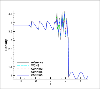
(a) Density on the area $[-5.00,5.00]$,

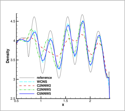
(b) Density on the area $[0.5,2.4]$,

Figure 11: Density distributions of single schemes in solving Shu-Osher problem ($T=1.8$, $DOFs=400$).

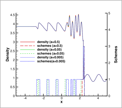
(a) Distribution of density and schemes of HCCS(1,1,1,1)

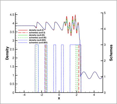
(b) Distribution of density and schemes of HCCS(1,0,0,1)

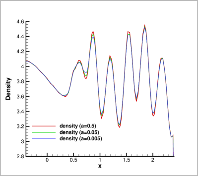
(c) Density on the area [−0.4,2.40] of HCCS(1,1,1,1)

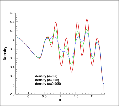
(d) Density on the area [−0.4,2.40] of HCCS(1,0,0,1)

Figure 12: Distribution of density and schemes for HCCS(1,1,1,1) and HCCS(1,0,0,1) in solving Shu-Osher problem. Here schemes 0, 1, 2, 3 represent CPR, C5NNW5, C2NNW5 and C2NNW2, correspondingly. ($T=1.8$, $DOFs=400$)

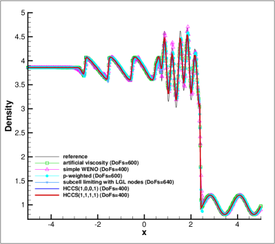
(a) Density on the area $[-5.00,5.00]$,

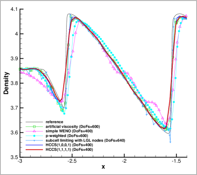
(b) Density on the area $[-3.00,-1.40]$

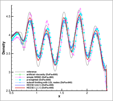
(c) Density on the area $[0.50,2.40]$

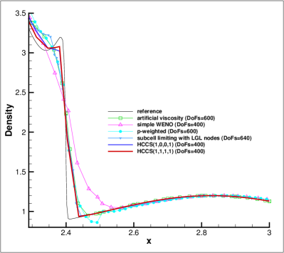
(d) Density on area $[2.29,3.00]$

Figure 13: Comparison of hybrid schemes HCCS(1,1,1,1) and HCCS(1,0,0,1) with artificial viscosity approach in Discacciati et al. [12], simple WENO limiter in Li et al. [20], $p$-weighted limiter in Li et al. [20] and subcell shock capturing based on LGL nodes in Hennemann et al. [30] for solving 1D Euler equations.

6.4 2D Euler vortex problem

In this subsection, the isentropic vortex problem in reference Hu and Shu [32] is solved to test order of accuracy, time evolution of numerical errors and discrete conservation properties of the proposed schemes. The initial condition is a mean flow with $\{\rho,u,v,p\}=\{1,1,1,1\}$. An isotropic vortex is then added to the mean flow with perturbations in $u,v$ and $T=p/\rho$ but a constant entropy $S=p/\rho^{\gamma}$:

$$\left(\Delta u,\Delta v\right) = \frac{\varepsilon}{2\pi}e^{0.5(1-r^{2})}(-y,x),$$

$$\Delta T = -\frac{(\gamma-1)\varepsilon^{2}}{8\gamma\pi^{2}}e^{1-r^{2}},$$

with $r=\sqrt{x^{2}+y^{2}}$ and the vortex strength $\varepsilon=5$. In the numerical simulations, the computational domain is taken to be $[-10,10]\times[-10,10]$ with periodic boundary conditions. Here errors of density are adopted in calculating numerical errors.

Firstly, the fifth-order linear schemes, CPR5, C5NNW5 with linear weights and WCNS5 with linear weights, are used to solve this problem till $T=dt$ and $T=2$ with a time step of $dt=0.0001$. Tabs. 7 and 8 present numerical errors of density and orders of accuracy for different schemes. At $T=dt$, C5NNW5 and CPR5 have fourth-order of accuracy while WCNS5 has fifth-order of accuracy and the smallest numerical errors. At $T=2$, C5NNW5 and WCNS5 can obtain fifth-order of accuracy which is higher than that of CPR5. However, the CPR5 has the smallest numerical errors. To further study the time evolution of errors, the time evolution of numerical errors and orders of accuracy are presented in Fig. 14 for the three schemes. We can see that the numerical errors of the CPR5 grows slower in time than the WCNS5 and C5NNW5, which illustrates the reason that WCNS5 has smaller error than CPR5 at $T=dt$ while has larger numerical errors than CPR5 at $T=2$.

Secondly, the fifth-order nonlinear schemes C5NNW5 and WCNS5 are taken to solve this problem till $T=2$ by taking JS weights with $\epsilon=10^{-6}$. From Table 9 we can see that schemes using nonlinear weights on characteristic variables have larger numerical errors than that on primary variables. In addition, both of C5NNW5 and WCNS5 can still acquire fifth-order of accuracy and C5NNW5 has a bit larger numerical errors than WCNS5.

Thirdly, the influence of indicating on accuracy of CPR-CNNW schemes is tested. A special threshold value $c_{1}=c(0.0005)$ is considered, which makes some cells in smooth regions being indicated wrongly as troubled cells. HCCS(1,1,1,1) with $\mathbf{dv}=(c_{1},0.05,0.1)$ and HCCS(1,0,0,1) with $\mathbf{dv}=(c_{1},c_{1},c_{1})$ are applied to solve this problem by using characteristic variables in NNW interpolations. The numerical errors and CPU times are given in Table 10. We can see that HCCS(1,1,1,1) still have nearly fifth-order of accuracy while HCCS(1,0,0,1) has second-order of accuracy, which illustrates that indicating wrongly has less influences on accuracy of HCCS(1,1,1,1) than that of HCCS(1,0,0,1). In addition, HCCS(1,1,1,1) and HCCS(1,0,0,1) have similar CPU time, which is nearly 111% of pure CPR5 schemes for the grid with $\sqrt{DOFs}=800$.

$Norm$	$\sqrt{DOFs}$	C5NNW5		CPR5		WCNS5
		error	order	error	order	error	order
$L_{\infty}$	$100$	1.38E-07	-	7.33E-07	-	6.52E-08	-
	$200$	1.03E-08	3.74	9.24E-08	2.99	2.46E-09	4.73
	$400$	6.69E-10	3.94	7.36E-09	3.65	8.09E-11	4.93
	$800$	4.11E-11	4.02	4.71E-10	3.97	2.57E-12	4.98
$L_{2}$	$100$	7.15E-09	-	4.57E-08	-	4.12E-09	-
	$200$	3.91E-10	4.19	3.65E-09	3.65	1.47E-10	4.81
	$400$	2.31E-11	4.08	2.50E-10	3.87	4.76E-12	4.95
	$800$	1.43E-12	4.01	1.59E-11	3.97	1.50E-13	4.99

Table 7: Comparisons of linear schemes based on original physical variables in solving 2D vortex problem ($T=dt=0.0001$).

$Norm$	$\sqrt{DOFs}$	C5NNW5		CPR5		WCNS5
		error	order	error	order	error	order
$L_{\infty}$	$100$	1.71E-3	-	3.00E-4	-	1.56E-3	-
	$200$	7.08E-5	4.59	7.58E-6	5.31	5.24E-5	4.90
	$400$	2.88E-6	4.62	5.55E-7	3.77	1.64E-6	5.00
	$800$	9.69E-8	4.89	2.70E-8	4.36	5.13E-8	5.00
$L_{2}$	$100$	6.83E-5	-	1.29E-5	-	5.30E-5	-
	$200$	2.35E-6	4.86	4.44E-7	4.86	1.89E-6	4.81
	$400$	8.68E-8	4.76	2.57E-8	4.11	6.09E-8	4.96
	$800$	2.62E-9	5.05	1.31E-9	4.29	1.91E-9	4.99

Table 8: Comparisons of linear schemes based on original physical variables in solving 2D vortex problem ($T=2$).

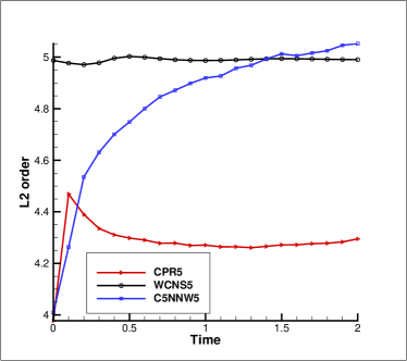
(a) Time evolution of L2 accuracy order based on $DOFs=400$ and $DOFs=800$, $t_{k}=0.0001,0.2,0.4,0.6,0.8,...,2.0$.

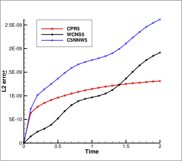
(b) Time evolution of L2 numerical error ($DOFs=800$)

Figure 14: Time evolution of numerical accuracy order and numerical errors ($T=2$)

$Norm$	$\sqrt{DOFs}$	Primary variables				Characteristic variables
		C5NNW5		WCNS5		C5NNW5		WCNS5
		error	order	error	order	error	order	error	order
$L_{\infty}$	$100$	4.41E-03	-	3.08E-03	-	1.12E-02	-	7.63E-03	-
	$200$	1.97E-04	4.48	1.55E-04	4.31	4.43E-04	4.66	2.80E-04	4.77
	$400$	9.18E-06	4.42	5.65E-06	4.78	8.40E-06	5.72	3.98E-06	6.14
	$800$	3.06E-07	4.91	1.79E-07	4.98	3.57E-07	4.56	1.46E-07	4.77
$L_{2}$	$100$	2.17E-04	-	1.39E-04	-	3.70E-04	-	2.44E-04	-
	$200$	9.27E-06	4.55	6.73E-06	4.37	1.95E-05	4.25	1.15E-05	4.41
	$400$	3.54E-07	4.71	2.43E-07	4.79	4.27E-07	5.51	2.54E-07	5.50
	$800$	1.11E-08	5.00	7.98E-09	4.93	1.35E-08	4.98	8.95E-09	4.83

Table 9: Comparisons of nonlinear schemes based on primary variables and characteristic variables in solving 2D vortex problem ($T=2$).

$Norm$	$\sqrt{DOFs}$	CPR-CNNW schemes						Single scheme
		HCCS(1,1,1,1)			HCCS(1,0,0,1)			CPR5
		error	order	CPU (s)	error	order	CPU (s)	CPU (s)
$L_{\infty}$	$100$	6.01E-03	-	64.5312	3.3057E-02	-	64.6875	52.2656
	$200$	3.41E-04	4.13	330.5469	7.4320E-03	2.15	330.0938	278.1406
	$400$	7.45E-06	5.52	1421.4531	1.5424E-03	2.27	1412.9844	1279.2812

Table 10: Comparisons of numerical errors and CPU time of HCCS(1,1,1,1) and HCCS(1,0,0,1) in solving 2D vortex problem ($T=2$).

Fourthly, discrete conservation properties are tested for both single schemes and the hybrid CPR-CNNW schemes. The discrete conservation error is defined as the relative error in the preservation of the integral of the conservative quantity $\rho$:

$$\left\langle\rho\right\rangle=\frac{\int_{V}(\rho-\rho_{0})dxdy}{\int_{V}\rho_{0}dxdy}=\frac{\int_{V}(\rho-\rho_{0})Jd\xi d\eta}{\int_{V}\rho_{0}Jd\xi d\eta}=\frac{INT(\rho)-INT(\rho_{0})}{INT(\rho_{0})}$$

where $\rho$ and $\rho_{0}$ denote the density at the final time and the initial time, correspondingly. Here $V$ indicates the whole computational domain and $INT(\rho)=\int_{V}\rho Jd\xi d\eta$, which is estimated by

$$\sum_{i,j}\left(\sum_{l}\sum_{m}w_{l}w_{m}\rho_{i,j,l,m}J_{i,j,l,m}\right)\Delta\xi\Delta\eta,$$

for all schemes, where $w_{l}$ are the weights of the quadrature rule. In order to test discrete conservation of CPR-CNNW schemes, a special threshold value $c_{1}=c(0.0005)=0.0005\cdot 10^{-1.8(6+1)^{1/4}}\thickapprox 5.9\times 10^{-7}$ is taken. Then, HCCS(1,1,1,1) with $\mathbf{dv}=(c_{1},5\times 10^{-6},10^{-5})$ and HCCS(1,0,0,1) with $\mathbf{dv}=(c_{1},c_{1},c_{1})$ are applied to maintain that both CPR and CNNW are used in the computations. The density distribution, error distribution, scheme distribution and time evolution of the error $\left\langle\rho\right\rangle$ of HCCS(1,1,1,1) are shown in Fig. 15. We can see that the obtained flow is smooth and four schemes are adopted in the computation. In addition, the error $\left\langle\rho\right\rangle$ keeps almost zero. Errors in the conservation $\left\langle\rho\right\rangle$ are also summarized in Tab. 11 with $INT(\rho_{0})\approx 398.241743560187$ for this problem. All the conservation errors are at the level of rounding errors, which indicates that all the schemes satisfy discrete conservation.

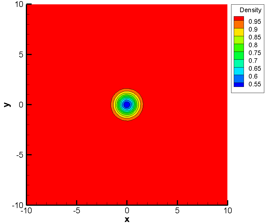
(a) Density distribution at $T=20$.

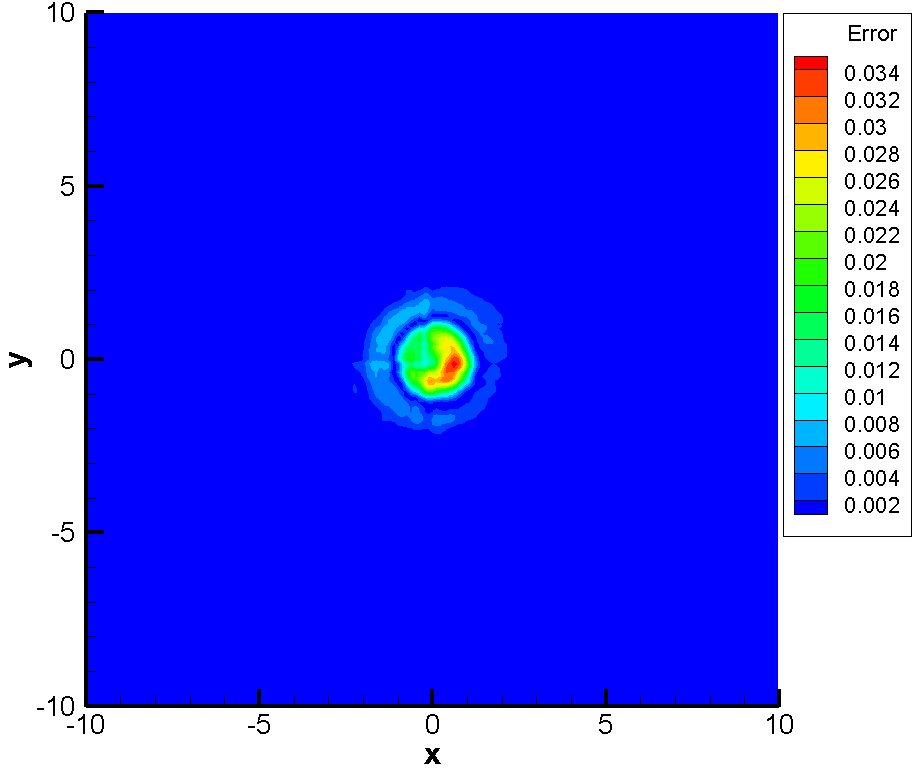
(b) Error distribution at $T=20$.

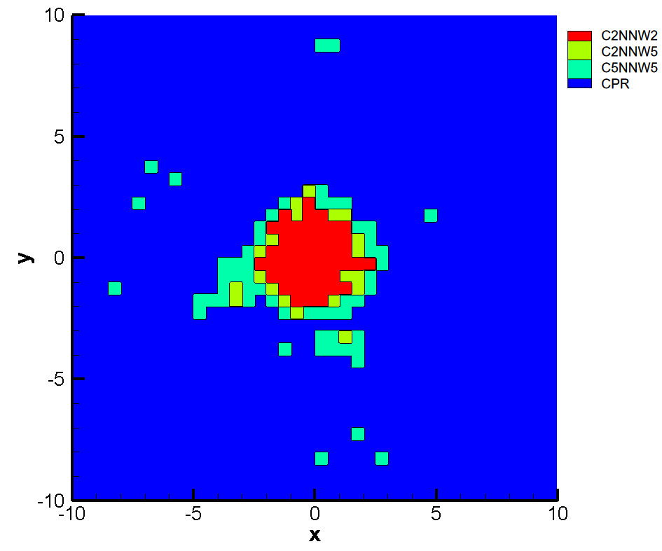
(c) Scheme distribution at $T=20$.

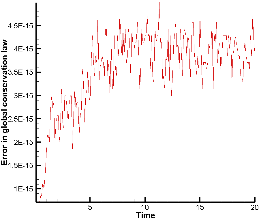
(d) Time evolution of the error $\left\langle\rho\right\rangle$.

Figure 15: HCCS(1,1,1,1) with $\mathbf{dv}=(c_{1},0.000005,0.00001)$ for solving Euler vortex problem ($40\times 40$ grid, $DOFs=200\times 200$, $dt=0.001$).

Schemes	CPR	C5NNW5	C2NNW5	C2NNW2	HCCS(1,1,1,1)	HCCS(1,0,0,1)
$\left\langle\rho\right\rangle_{max}$	4.42E-15	3.57E-15	3.71E-15	4.42E-15	5.00E-15	5.00E-15

Table 11: The maximum of $\left\langle\rho\right\rangle$ on time samples $t_{i}\in\left\{0.1i|i=1,2,\cdots,200\right\}$ for all schemes ($40\times 40$ grid, $dt=0.001$, $T=20$)

6.5 2D Riemann problem

The CNNW and CPR-CNNW schemes are applied to solve 2D Riemann problem proposed by Schulz-Rinne Schulz-Rinne [49]. The computational domain $\left[0,1\right]\times[0,1]$ is divided into four quadrants by two lines $x=0.8$ and $y=0.8$ and the initial constant states on the four quadrants are

$$(\rho,u,\upsilon,p) = \begin{cases}\mathbf{V_{\mathit{\mathrm{1}}}=}(\rho_{1},u_{1},\upsilon_{1},p_{1}),&0.8\leq x\leq 1.0,\,\,0.8\leq y\leq 1.0,\\ \mathbf{V}_{2}=(\rho_{2},u_{2},\upsilon_{2},p_{2}),&0.0\leq x<0.8,\,\,0.8\leq y\leq 1.0,\\ \mathbf{V}_{3}=(\rho_{3},u_{3},\upsilon_{3},p_{3}),&0.0\leq x<0.8,\,\,0.0\leq y<0.8,\\ \mathbf{V}_{4}=(\rho_{4},u_{4},\upsilon_{4},p_{4}),&0.8<x\leq 1.0,\,\,0.0\leq y<0.8.\end{cases}$$

Firstly, we test shock capturing properties for CNNW in solving the 2D Riemann problem with the initial constant states

$$\begin{array}[]{cccc}&\mathbf{V}_{1}=(1.500,0,0,1.500),&&\mathbf{V}_{2}=(0.5323,1.206,0,0.3),\\ &\mathbf{V}_{3}=(0.138,1.206,1.206,0.029),&&\mathbf{V}_{4}=(0.5323,0,1.206,0.3),\end{array}$$ (48)

till $T=0.8$. From Fig. 16, we can see that C5NNW5 has higher resolution than WCNS5 in capturing the vortices along the shear layers. For second-order schemes, C2NNW5 captures more small scale features than C2NNW2, which illustrates that the former has higher resolution than the latter.

Secondly, HCCS(1,1,1,1) with $\mathbf{dv}=(c(a),0.3,0.6)$ and HCCS(1,0,0,1) with $\mathbf{dv}=(c(a),c(a),c(a))$ are adopted to solve this problem. The results in Fig. 17 and Fig. 18 show that both of HCCS(1,1,1,1) and HCCS(1,0,0,1) can capture shocks effectively and the former which contain C5NNW5 and C2NNW5 captures more flow structures than the latter. In addition, HCCS(1,1,1,1) can keep high resolution when increasing the number of troubled cells as shown in Fig. 17. HCCS(1,0,0,1) can not acquire small-scale features since when the shear wave or vortex structures are indicated wrongly, they are limited by the dissipative C2NNW2, which smears out the small scale vortex structures.

(a) C5NNW5

(b) WCNS5

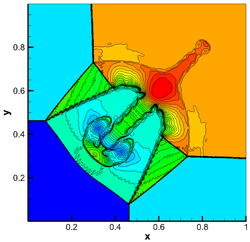
(c) C2NNW5

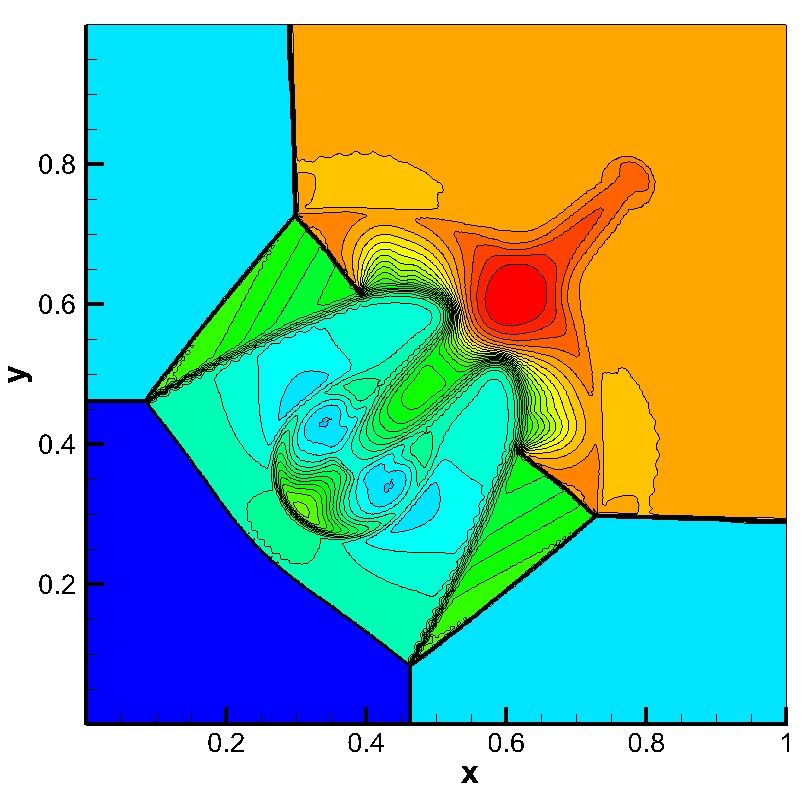
(d) C2NNW2

Figure 16: Density from 0.2 to 1.7 with 31 contours computed by C5NNW5, WCNS5, C2NNW5, C2NNW2 ($120\times 120$ grid, $DOFs=600\times 600$, $T=0.8$)

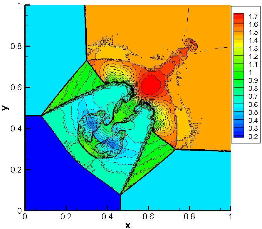
(a) Density contours, $a=0.5$

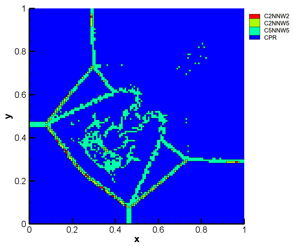
(b) Distribution of different cells, $a=0.5$

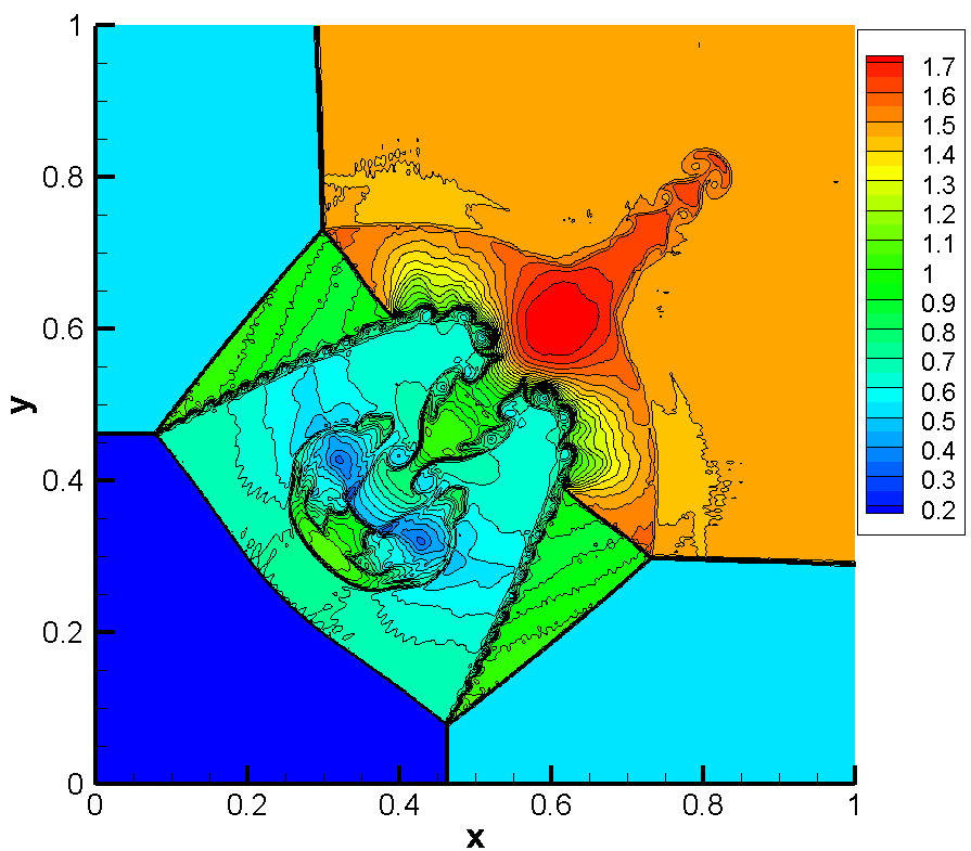
(c) Density contours, $a=0.05$

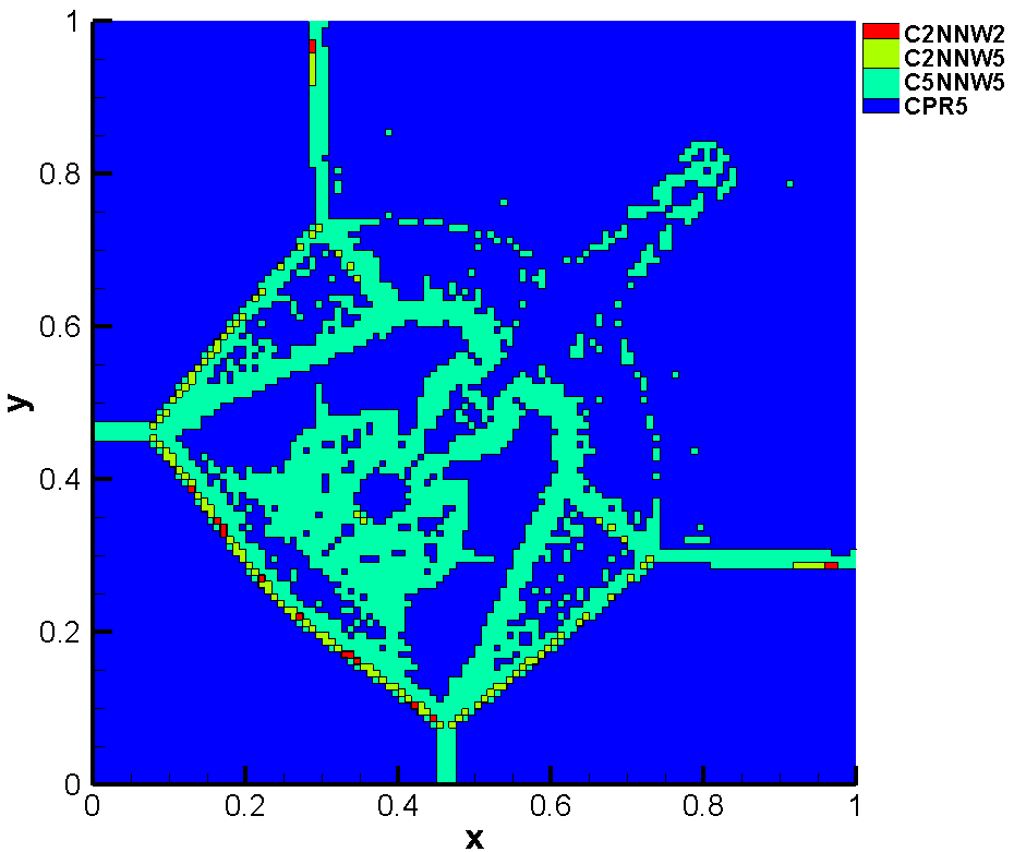
(d) Distribution of different cells, $a=0.05$

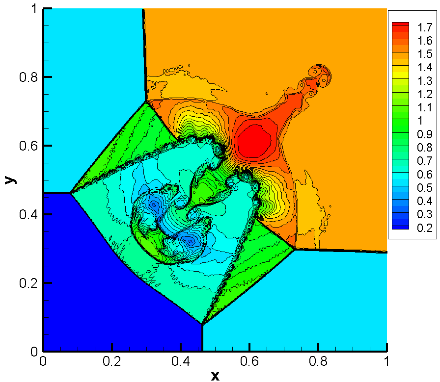
(e) Density contours, $a=0.005$

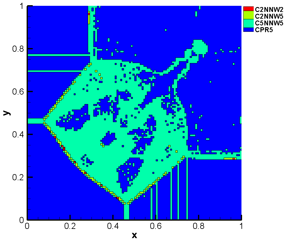
(f) Distribution of different cells, $a=0.005$

Figure 17: 2D Riemann problem solved by HCCS(1,1,1,1) with $\mathbf{dv}=(c(a),0.3,0.6)$. Density from 0.2 to 1.7 with 31 contours and distribution of different cells. ($120\times 120$ grid, $DOFs=600\times 600$, $T=0.8$)

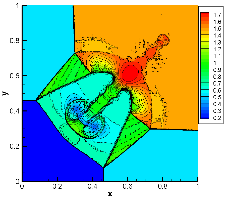
(a) Density contours, $a=0.5$

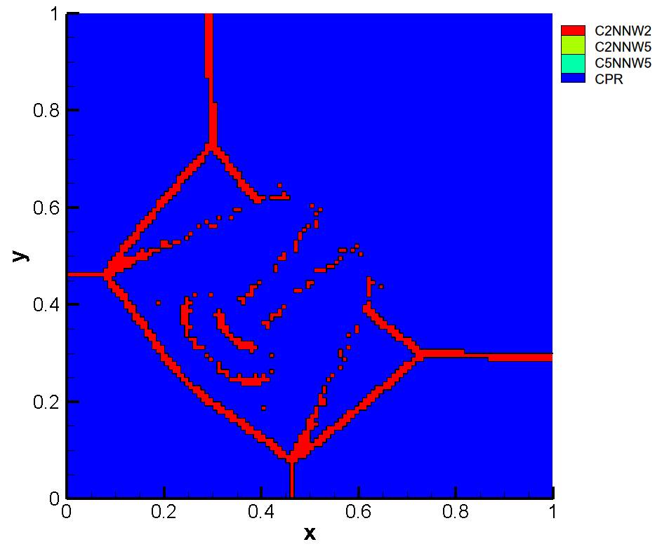
(b) Distribution of different cells, $a=0.5$

(c) Density contours, $a=0.05$

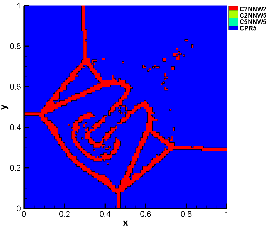
(d) Distribution of different cells, $a=0.05$

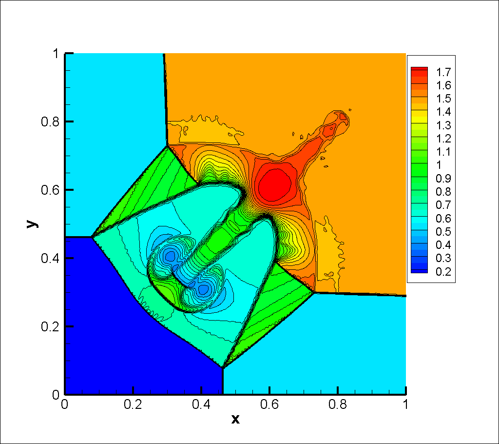
(e) Density contours, $a=0.005$

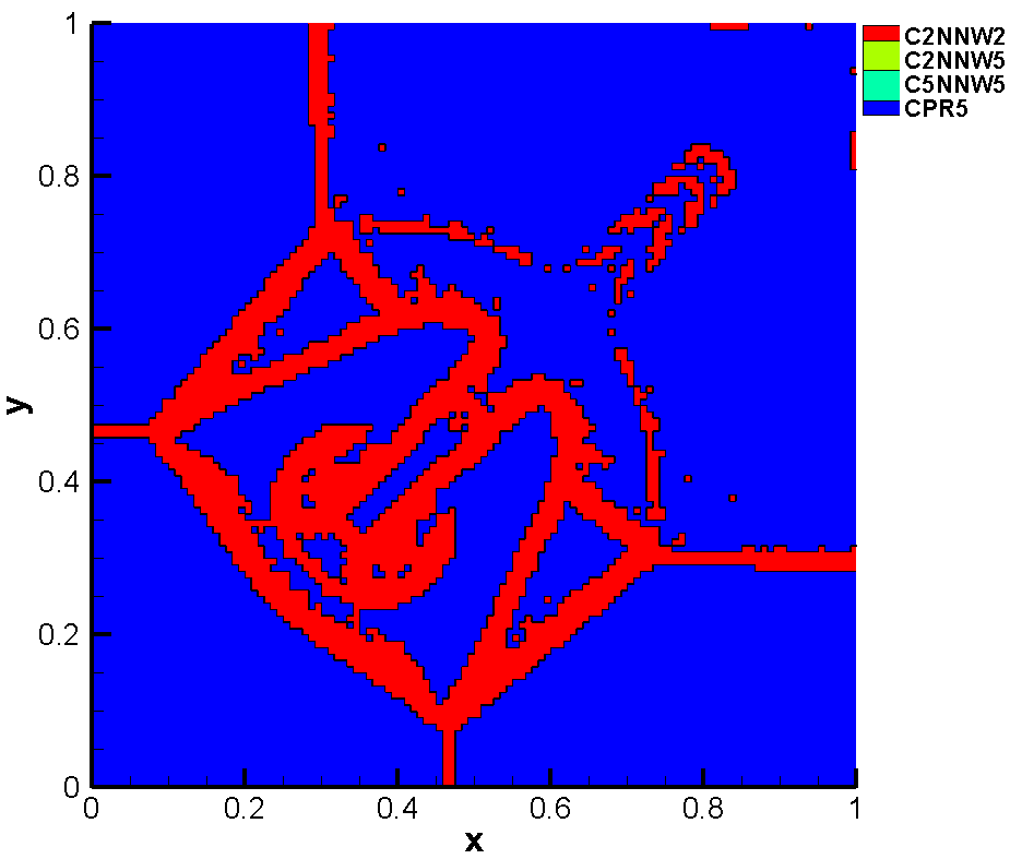
(f) Distribution of different cells, $a=0.005$

Figure 18: 2D Riemann problem solved by HCCS(1,0,0,1) with $\mathbf{dv}=(c(a),c(a),c(a))$. Density from 0.2 to 1.7 with 31 contours and distribution of different cells ($120\times 120$ grid, $DOFs=600\times 600$, $T=0.8$)

At last, we change shock strength of the Riemann problem to test shock capturing ability of CNNW and CPR-CNNW. The initial constant states are

$$\begin{cases}\rho_{3}&=0.138,\\ u_{3}&=M\sqrt{\frac{\gamma p_{3}}{\rho_{3}}}/\sqrt{2},\\ \upsilon_{3}&=u_{3},\\ p_{3}&=0.029,\end{cases} \begin{cases}s_{23}&=\frac{3-\gamma}{4}\upsilon_{3}-\sqrt{\frac{\gamma p_{3}}{\rho_{3}}+\left[\frac{\left(\gamma+1\right)}{4}\upsilon_{3}\right]^{2}},\\ \rho_{2}&=-\frac{\rho_{3}\upsilon_{3}}{s_{23}}+\rho_{3},\\ u_{2}&=u_{3},\\ \upsilon_{2}&=0,\\ p_{2}&=(\rho_{3}\upsilon_{3}^{2}+p_{3})-s_{23}\rho_{3}\upsilon_{3},\end{cases}$$

$$\begin{cases}\rho_{4}&=\rho_{2},\\ u_{4}&=0,\\ \upsilon_{4}&=u_{2},\\ p_{4}&=p_{2},\end{cases} \begin{cases}s_{12}&=\frac{3-\gamma}{4}u_{2}-\sqrt{\frac{\gamma p_{2}}{\rho_{2}}+\left[\frac{\left(\gamma+1\right)}{4}u_{2}\right]^{2}},\\ \rho_{1}&=-\frac{\rho_{2}u_{2}}{s_{12}}+\rho_{2},\\ u_{1}&=0,\\ \upsilon_{1}&=0,\\ p_{1}&=(\rho_{2}u_{2}^{2}+p_{2})-s_{12}\rho_{2}u_{2}.\end{cases}$$

The shock Mach $M=\sqrt{2}u_{3}/\sqrt{\gamma p_{3}/\rho_{3}}$ here is an adjustable parameter to control the shock strength and the states $\mathbf{V}_{2}$,$\mathbf{V}_{4}$ and $\mathbf{V}_{1}$ are determined based on the Rankine-Hugoniot condition. Please note that the initial conditions of 48 is a special case of $M=3.145$ with possible rounding errors. In our tests, $M$ is changed gradually from $3.145$ to $10^{6}$ to test whether a numerical scheme can capture the shocks without blowing up. The largest $M$ for different schemes without blowing up are summarized in Table 12.

In the C5NNW5, nonlinear mechanism is introduced in the interpolation process (from solution points to flux points). However, the compact flux difference operator (C5) still relies on an uniform polynomial assumption, which is known to result in Gibbs phenomenon near discontinuities. The resulting C5NNW5 can calculate problems with $M<6$. Even if we introduce constant interpolation (NNW1), which was shown to be very dissipative in the communities of finite difference and finite volume studies, such as var Leer [43], Buffard and Clain [50], Zhu et al. [41], the resulting C5NNW1 still blows up at about $M=8.2$. This indicates that it maybe impossible to construct a high-order FE schemes capable of simulating very strong shocks by introducing nonlinear mechanism to only parts of the operators that are based on uniform polynomial assumption, which is fundamental in high-order FE schemes like CPR and DG. In another word, a possible reason for the difficulty in constructing robust shock capturing high-order FE methods using the artificial viscosity Persson and Peraire [11], Yu and Hesthaven [13] or limiting solution distribution Zhu and Qiu [17], Zhong and Shu [9], Zhu et al. [18], Du et al. [19], Park and Kim [21], Li et al. [20] is that the nonlinear mechanism only breaks the uniform polynomial assumption in parts of the high-order FE methods. However, the remaining operators based on uniform polynomial still generates oscillations and easily leads to blow up.

The C2NNW5 scheme, which breaks the uniform polynomial distribution assumption for both interpolation and flux difference operators using NNW5 and C2 respectively, successfully captures shocks with $M=10^{6}$ and a much more robust shock capturing ability is obtained. We can see that second-order schemes C2NNW5 and C2NNW2 can compute stronger shocks than high-order schemes C5NNW5. Based on this observation, it is better for hybrid schemes to contain low-order robust shock capturing schemes to capture strong shocks.

In our subcell limiting strategy, we can divide the high-order CPR cells into subcells computed by second-order schemes C2NNW5 and C2NNW2 for strong shocks, and therefore break the uniform polynomial distribution assumption for every operators. From Table 12, we can see that the HCCS(1,1,1,1) with $\mathbf{dv}=(c_{0},0.005,0.01)$ and HCCS(1,0,0,1) with $\mathbf{dv}=(c_{0},c_{0},c_{0})$ can calculate this problem with $M=10^{6}$, which illustrate that the proposed CPR-CNNW have good properties in capturing strong shocks.

Schemes	Low-order schemes			Fifth-order schemes		CPR-CNNW
	C5NNW1	C2NNW5	C2NNW2	C5NNW5	WCNS5	HCCS(1,1,1,1)	HCCS(1,0,0,1)
$M_{max}$	8.2	$10^{6}$	$10^{6}$	6.0	183	$10^{6}$	$10^{6}$

Table 12: Comparisons of nonlinear schemes in solving 2D Riemann problems with different Ma.

6.6 Double Mach reflection

Double Mach reflection problem described in Woodward and Colella [51] is a popular test case to test strong shock capturing ability of high-resolution schemes. The problem is solved by CPR-CNNW schemes on a grid with $h=1/108$. As shown in Fig. 19, CPR-CNNW schemes can capture strong shock robustly. In addition, HCCS(1,1,1,1) can capture small-scale structures better than HCCS(1,0,0,1). Comparing Fig. 19(b) and (d), we can see HCCS(1,1,1,1) computes the troubled cells with strong shocks using C2NNW2 while using C2NNW5 and C5NNW5 for weak discontinuities and cells next to discontinuities. However, HCCS(1,0,0,1) compute all these cells by the C2NNW2. These results illustrate that HCCS(1,1,1,1) containing C5NNW5 and C2NNW5 can acquire higher resolution than HCCS(1,0,0,1).

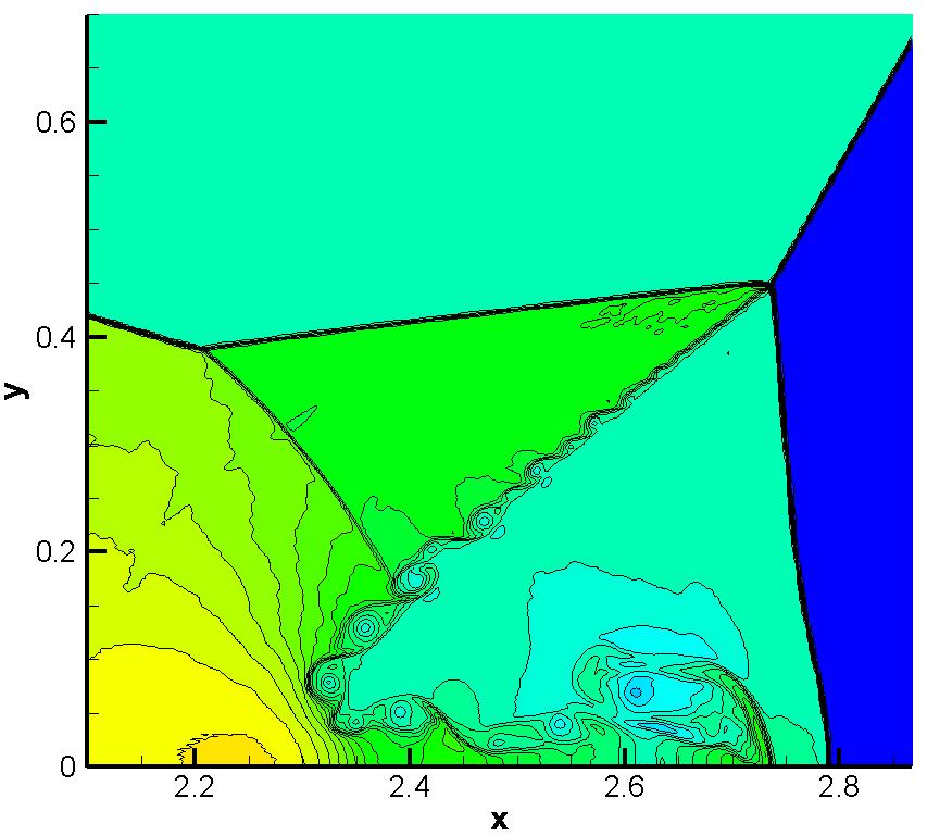
(a) HCCS(1,1,1,1), density from 1.5 to 21.7 with 31 contours.

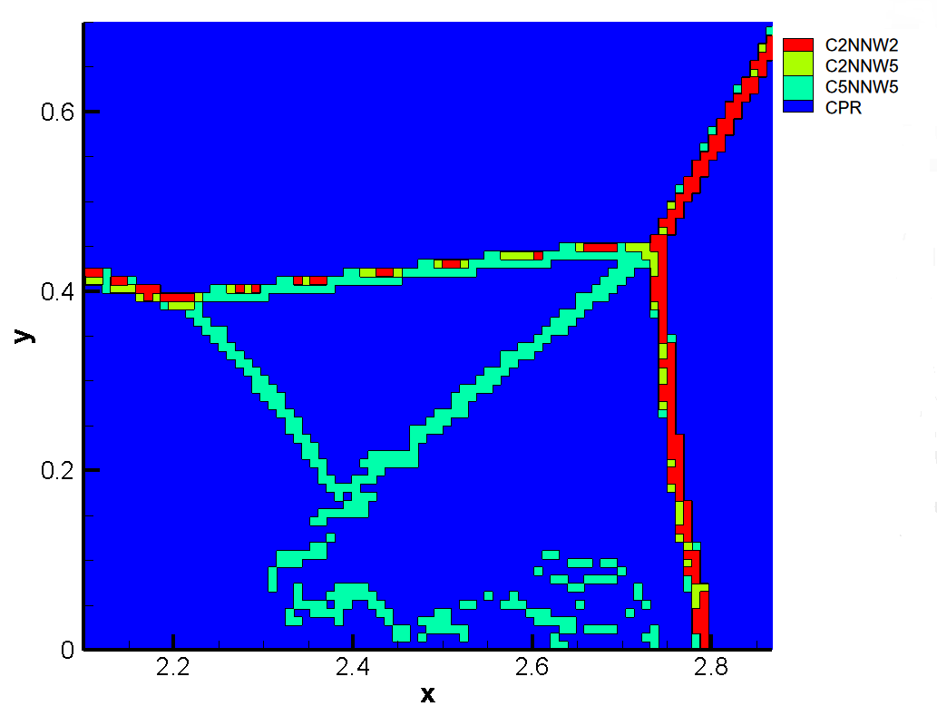
(b) HCCS(1,1,1,1), distribution of different cells

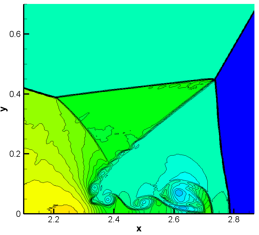
(c) HCCS(1,0,0,1), density from 1.5 to 21.7 with 31 contours.

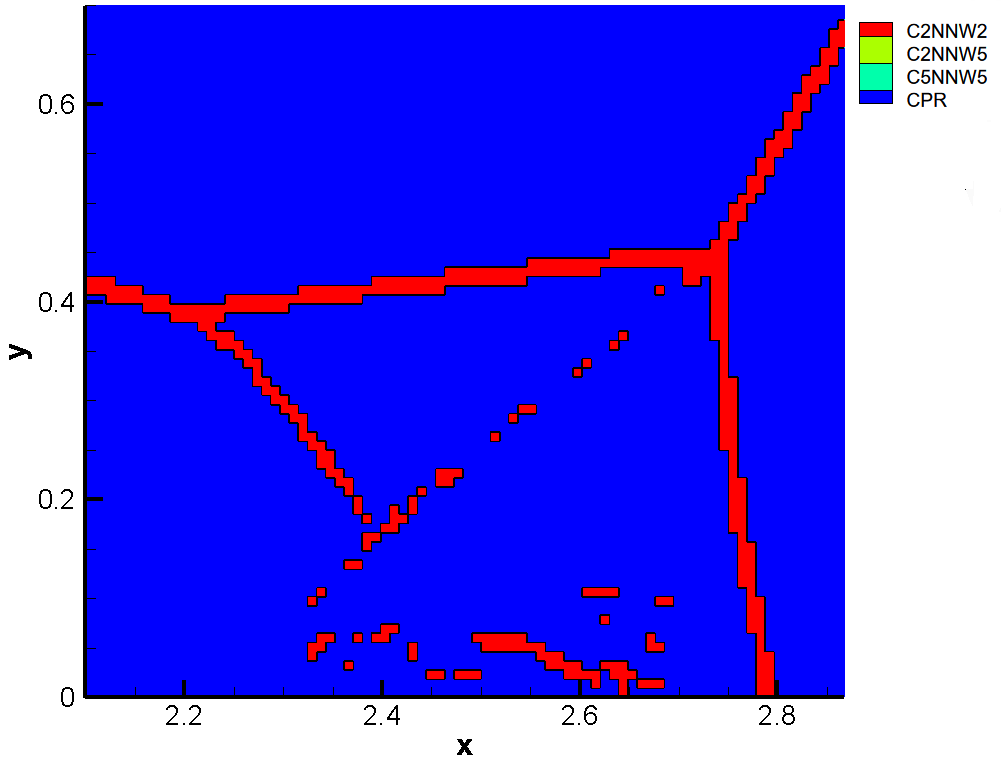
(d) HCCS(1,0,0,1), distribution of different cells

Figure 19: Hybrid scheme HCCS(1,1,1,1) with $\mathbf{dv}=(c_{0},0.05,0.1)$ and HCCS(1,0,0,1) with $\mathbf{dv}=(c_{0},c_{0},c_{0})$ in solving Double Mach reflection problem ($h=1/108$, $DOFs=2160\times 540$, $T=0.2$)

6.7 Shock-vortex interaction

As a final test, shock-vortex interaction is solved by CPR-CNNW schemes to test their good balance in shock capturing and high resolution. This test case is originally proposed by Rault et al. [52] and is one of the benchmark problems of the 5th International Workshop on High Order CFD Methods (HiOCFD5). It has been adopted as a benchmark for high-order numerical schemes Dumbser and M. Kaser [53], Dumbser et al. [24], You and Kim [54], since it involves a complex flow pattern with both smooth features and discontinuous waves. The computational domain is $[0,2]\times[0,1]$. The initial conditions are given by a stationary normal shock wave placed at $x=0.5$ with shock Mach number $M_{s}$ and by a vortex placed at $(x_{c},y_{c})=(0.5,0.5)$ with the strength $M_{v}$. We choose $M_{s}=1.5$ and $M_{v}=0.9$, which is the same as that in Rault et al. [52]. A computational grid with $h=1/140$ and $DoFs=1400\times 700=980000$ is used.

HCCS(1,1,1,1) and HCCS(1,0,0,1) are applied to solve this problem. The distribution of the density, of different cells and of the density derivatives at time $T=0.7$ are shown in Fig. 20 for HCCS(1,1,1,1) and in Fig. 21 for HCCS(1,0,0,1). The results show that the hybrid CPR-CNNW scheme can capture shock wave as well as smooth vortex features. Our results are comparable qualitatively with those computed by ADER-DG-P5 with a posteriori ADER-WENO3 subcell limiter Dumbser et al. [24] and with the numerical solution provided in Rault et al. [52]. In addition, density along five lines are also shown in Fig. 22. From Fig. 22(a) (b) (c), we can see that there are no obvious oscillations near the stationary shock wave at $x=0.5$. Vortical structures are also well simulated, as shown in Fig. 22(a) (e). Large scale flow structures are well resolved although there are some small shock-driven oscillations, as shown in 22(c) (d) (f). Density along Line 4 in Fig. 22(e) also shows that HCCS(1,1,1,1) can acquire better resolution in computing the vortical structure.

To view the influence of troubled cell detecting, the results of HCCS(1,1,1,1) and HCCS(1,0,0,1) with parameter $a=0.005$ are shown in Fig. 23. Under this parameter the vortex area is detected as troubled cells, as shown in Fig. 23(a)(c). We can see that the HCCS(1,1,1,1) can compute the vortical structure better than HCCS(1,0,0,1), as shown in Fig. 23(b) (d). Moreover, density along Line 1 and Line 4 are compared in Fig. 23(e) (f). We can see that HCCS(1,1,1,1) can keep high resolution when increasing the number of troubled cells (by increasing $a$) while the resolution of HCCS(1,0,0,1) decreases significantly.

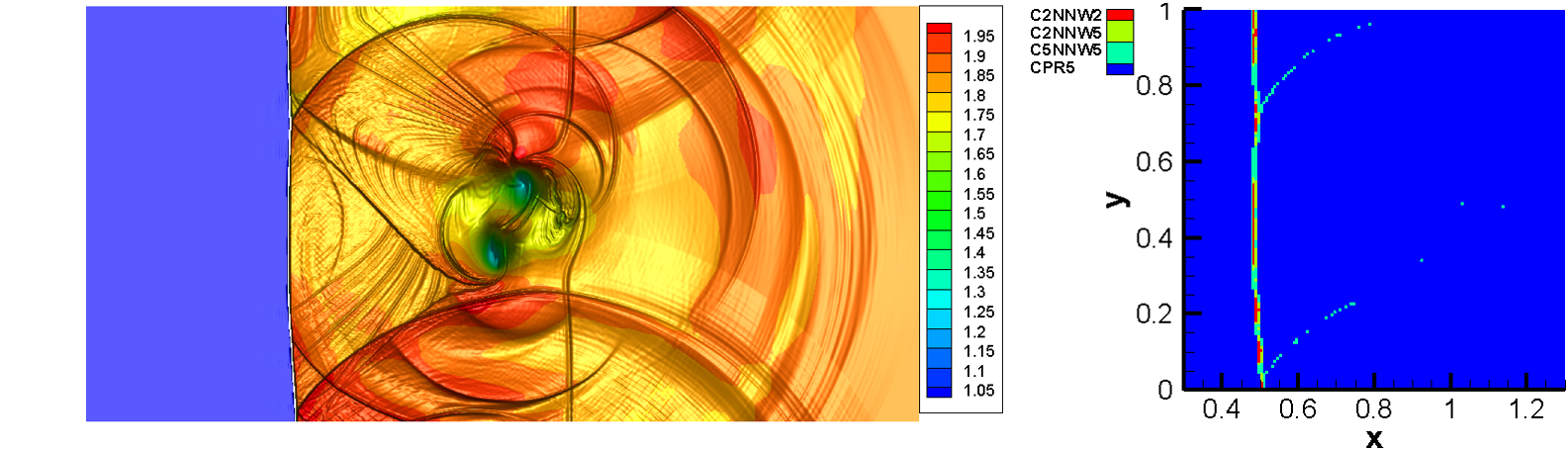
(a) Distribution of density and different cells

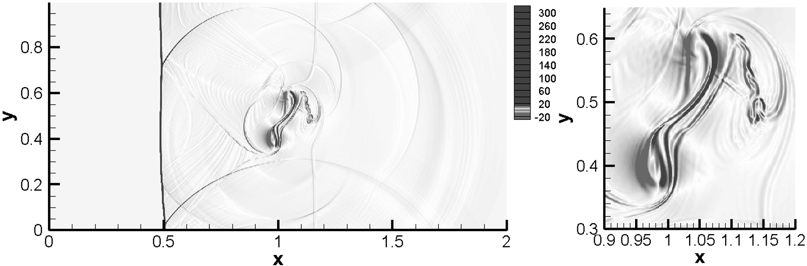
(b) Schlieren View of density and its close-up

Figure 20: Shock-vortex interaction problem solved by HCCS(1,1,1,1) with $\mathbf{dv}=(c_{0},0.05,0.1)$ ($h=1/140$, $DoFs=1400\times 700$, $T=0.7$)

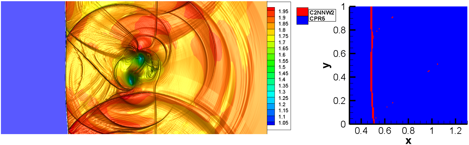
(a) Distribution of density and different cells

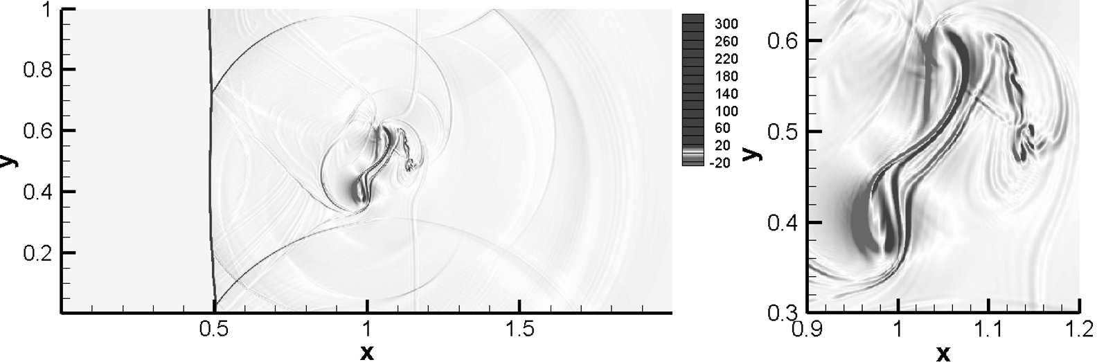
(b) Schlieren View of density and its close-up

Figure 21: Shock-vortex interaction problem solved by HCCS(1,0,0,1) with $\mathbf{dv}=(c_{0},c_{0},c_{0})$ ($h=1/140$, $DoFs=1400\times 700$, $T=0.7$)

(a) Density along Line 1 ($y=0.4$)

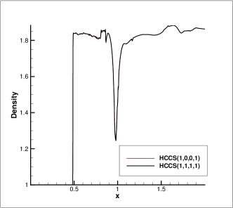
(b) Density along Line 1 ($y=0.4$) near shock on the area $x\in[0.47,0.51]$.

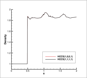
(c) Density along Line 2 ($y=0.7$)

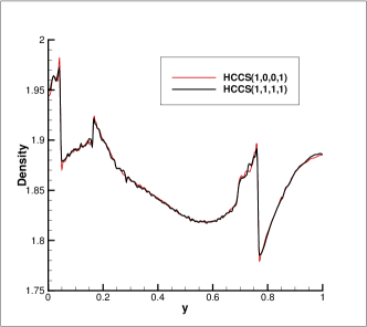
(d) Density along Line 3 ($x=0.52$)

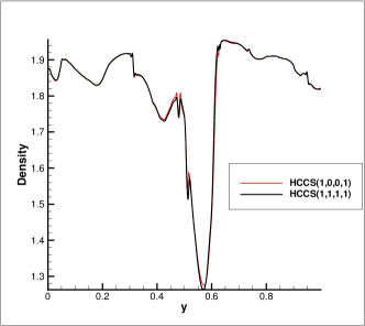
(e) Density along Line 4 ($x=1.05$)

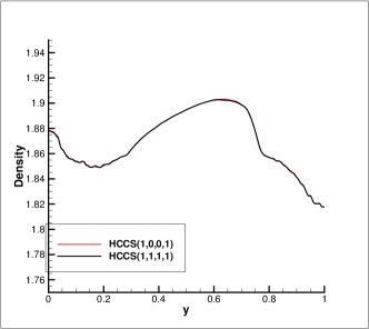
(f) Density along Line 5 ($y=1.65$)

Figure 22: Results along five lines of HCCS(1,1,1,1) with $\mathbf{dv}=(c_{0},0.05,0.1)$ and HCCS(1,0,0,1) with $\mathbf{dv}=(c_{0},c_{0},c_{0})$ where $a=0.5$ in solving shock-vortex interaction ($h=1/140$, $DoFs=980000$, $T=0.7$).

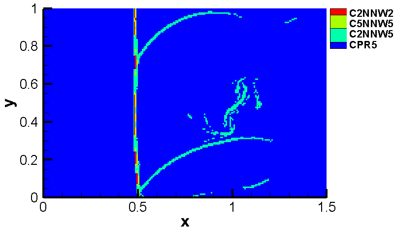
(a) Distribution of different cells, HCCS(1,1,1,1)

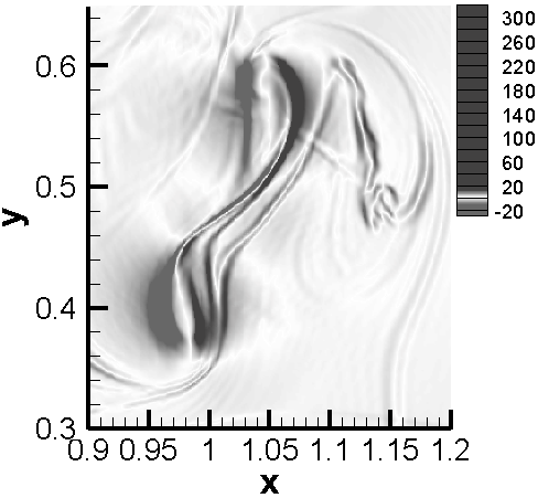
(b) Schlieren View, HCCS(1,1,1,1)

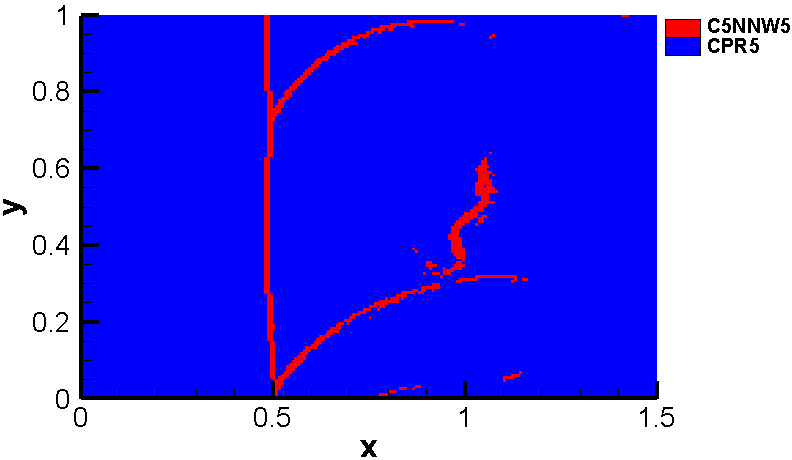
(c) Distribution of different cells, HCCS(1,0,0,1)

(d) Schlieren View, HCCS(1,0,0,1)

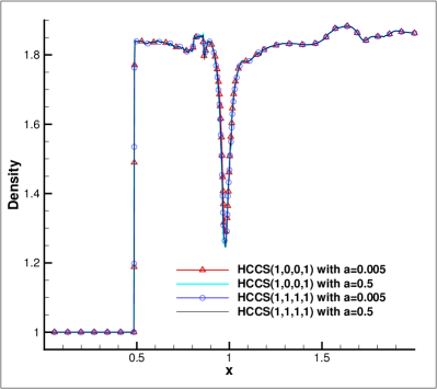
(e) Comparisons on Line 1.

(f) Comparisons on Line 4

Figure 23: Shock-vortex interaction problem solved by HCCS(1,1,1,1) with $\mathbf{dv}=(c(a),0.05,0.1)$ and HCCS(1,0,0,1) with $\mathbf{dv}=(c(a),c(a),c(a))$ where $a=0.005$. ($h=1/140$, $DoFs=1400\times 700$, $T=0.7$)

7 Concluding Remarks

In this paper, both high-order and second-order shock capturing schemes based on nonuniform nonlinear weighted interpolation are proposed and these schemes are applied in subcell limiting for the high-order CPR method. Eigenvalues of the spatial discretization matrix of the proposed high-order CNNW are proved to be a collection of eigenvalues of local matrices. All eigenvalues are computed and compared with CPR and WCNS. The results show that the proposed high-order CNNW schemes are stable and have similar spectral properties as those of WCNS. Then, a priori subcell CNNW limiting approach is developed for the fifth-order CPR, resulting in a special hybrid scheme and is called CPR-CNNW. To ensure robustness and accuracy of the hybrid scheme, CNNW schemes with varying accuracy orders are chosen adaptively according to the magnitude of troubled cell indicator. The proposed CNNW and CPR-CNNW schemes are applied to solve linear advection equation and Euler equations. Numerical investigations show that the proposed C5NNW5 have fifth-order of accuracy. C2NNW5 and C2NNW2 has second-order of accuracy and the former has higher resolution than the later one. In addition, C2NNW5 and C2NNW2 are more robust in shock capturing than fifth-order scheme C5NNW5. It is shown that the CPR with subcell $p$-adaptive CNNW limiting has higher resolution than subcell second-order C2NNW2 limiting, which illustrate that high-order interpolation in subcells can improve resolution. CPR with subcell $p$-adaptive CNNW limiting has good balance in high resolution and shock capturing. The scheme combines the advantages of high-order CPR schemes in smooth regions, with the robustness and accuracy of $p$-adaptive CNNW for shock capturing. Both analytical and numerical results show that the CPR-CNNW schemes satisfy discrete conservation law. The proposed hybrid CPR-CNNW has some merits in less data exchanging for physical variables, in satisfying discrete conservation laws, and in good balance between high resolution and good shock capturing robustness. The proposed subcell limiting approach could be generalized to CPR on unstructured meshes by making some changes in interpolation procedure. The limiting approach in theory can be applied to DG or other kind of FE method.

Appendix A. NNW5 interpolation

Here we give fifth-order nonuniform nonlinear weighted interpolation in one-dimensional case for obtaining the right values at the first flux point of the $i$th cell $u_{i,fp_{1}}^{R}$based on the stencil of the first solution point $sp_{1}$, where $fp_{1}$ and $sp_{1}$ denote the first flux point and the first solution point at the $i$th cell, correspondingly. The values at other flux points can be obtained by similar procedure.

Step A: Choose a stencil of five points $S_{i,sp_{1}}=\{u_{i-1,sp_{4}},u_{i-1,sp_{5}},u_{i,sp_{1}},u_{i,sp_{2}},u_{i,sp_{3}}\}$ and divide this stencil into three small stencil $S_{i,sp_{1}}^{(1)}=\{u_{i-1,sp_{4}},u_{i-1,sp_{5}},u_{i,sp_{1}}\}$, $S_{i,sp_{1}}^{(2)}=\{u_{i-1,sp_{5}},u_{i,sp_{1}},u_{i,sp_{2}}\}$ and $S_{i,sp_{1}}^{(3)}=\{u_{i,sp_{1}},u_{i,sp_{2}},u_{i,sp_{3}}\}$.

Step B: Construct Lagrange interpolation polynomial $p_{sp_{1}}^{(m)}(\xi)$ in each stencil $S_{i,sp_{1}}^{(m)},m=1,2,3$, we have

$$p_{sp_{1}}^{(1)}(\xi_{fp_{1}}^{R}) = c_{11}u_{i-1,sp4}+c_{12}u_{i-1,sp5}+c_{13}u_{i,sp1},$$

$$p_{sp_{1}}^{(2)}(\xi_{fp_{1}}^{R}) = c_{21}u_{i-1,sp5}+c_{22}u_{i,sp1}+c_{23}u_{i,sp2},$$ (49)

$$p_{sp_{1}}^{(3)}(\xi_{fp_{1}}^{R}) = c_{31}u_{i,sp1}+c_{32}u_{i,sp2}+c_{33}u_{i,sp3}.$$

Step C: Calculate the linear weights $d_{m}$ for each stencil $S_{i,sp_{1}}^{(m)},m=1,2,3$. The fifth-order linear interpolation for obtaining $u_{i,fp_{1}}^{R}$can be obtained by Taylor expansion or Lagrange interpolation polynomial,

$$u_{i,fp_{1}}^{R} = a_{11}u_{i-1,sp4}+a_{12}u_{i-1,sp5}+a_{13}u_{i,sp1}+a_{14}u_{i,sp2}+a_{15}u_{i,sp3}$$ (50)

The linear weight are chosen to make the weighted results has optimal fifth-order of accuracy, thus

$$d_{1}(c_{11}u_{i-1,sp4}+c_{12}u_{i-1,sp5}+c_{13}u_{i,sp1})$$

$$+ d_{2}(c_{21}u_{i-1,sp5}+c_{22}u_{i,sp1}+c_{23}u_{i,sp2})$$

$$+ d_{3}(c_{31}u_{i,sp1}+c_{32}u_{i,sp2}+c_{33}u_{i,sp3}),$$

$$= a_{11}u_{i-1,sp4}+a_{12}u_{i-1,sp5}+a_{13}u_{i,sp1}+a_{14}u_{i,sp2}+a_{15}u_{i,sp3}.$$

Then, the linear weights $d_{1}$, $d_{2}$,$d_{3}$ can be determined. Coefficients and linear weights for fifth-order interpolation in (49) and (Appendix A. NNW5 interpolation) are given in Table 11. It is worth noticing that all of the linear weight are positive.

Step D: Compute smoothness indicator $IS_{m,sp_{1}}$ and nonlinear weights $\omega_{m}$ to get the NNW interpolation value at the flux points $\xi_{fp1}$,

$$u_{i,fp_{1}}^{R}=\sum_{m=1}^{3}\omega_{m}p_{sp_{1}}^{(m)}(\xi_{fp1}),$$

where $\left\{\omega_{1},\omega_{2},\omega_{3}\right\}$ are nonlinear weights. Various types of nonlinear weights have been developed, we refer to Jiang and Shu [31], Borges et al. [55], Yan et al. [56] and references therein. We consider two types of nonlinear weights in this paper. The first one is the JS weights Jiang and Shu [31], which are defined by

$$\omega_{m}=\frac{\beta_{m}}{\sum_{l=1}^{3}\beta_{l}},\quad\beta_{m}=\frac{d_{m}}{(\varepsilon+IS_{m,sp_{1}})^{2}},$$ (52)

where $\varepsilon=10^{-6}$ is a small number and $IS_{m,sp_{1}}$ is a smoothness indicator. The second one is the Z weights Borges et al. [55], which are defined by

$$\omega_{m}=\frac{\beta_{m}}{\sum_{l=1}^{3}\beta_{l}},\quad\beta_{m}=d_{m}\left(1+\frac{\left|IS_{3,sp_{1}}-IS_{1,sp_{1}}\right|^{2}}{(\varepsilon+IS_{m,sp_{1}})^{2}}\right),$$ (53)

where $\varepsilon=10^{-10}$ is a small number and $IS_{m,sp_{1}}$ is a smoothness indicator.

sp	fp	$\left\{d_{l}|l=1,2,3\right\}$, $\left\{c_{i,j}|i=1,2,3,\;j=1,2,3\right\}$
sp1	$u_{i,fp_{1}}^{R}$	$d_{1}^{1L}$=0.34210708229202832129514593919672	$c_{11}^{1L}$=-0.043104119062505851129386949103353
		$d_{2}^{1L}$=0.6308070429239803035449279980960	$c_{12}^{1L}$=0.62757338302641182681128438378820
		$d_{3}^{1L}$=0.027085874783991375159926062707238	$c_{13}^{1L}$=0.41553073603609402431810256531515
		$c_{21}^{1L}$=$c_{13}^{1L}$	$c_{31}^{1L}$=1.3850967572035142771188790865197
		$c_{22}^{1L}$=$c_{12}^{1L}$	$c_{32}^{1L}$=-0.47383715518113200994718334103294
		$c_{23}^{1L}$=$c_{11}^{1L}$	$c_{33}^{1L}$=0.088740397977617732828304254513256
	$u_{i,fp_{2}}^{L}$	$d_{1}^{1R}$=0.12849535271459107836474476379591	$c_{11}^{1R}$=0.22720313860956266078248678148547
		$d_{2}^{1R}$=0.7282735720676514895919532282452	$c_{12}^{1R}$=-1.4245445419469326647976617868947
		$d_{3}^{1R}$=0.14323107521775743204330200795893	$c_{13}^{1R}$=2.1973414033373700040151750054092
		$c_{21}^{1R}$=-0.30686122157984679047945926834897	$c_{31}^{1R}$=0.52024206914481960337059414500993
		$c_{22}^{1R}$=1.0796580829702841296969724868635	$c_{32}^{1R}$=0.54529095781405304293936341037295
		$c_{23}^{1R}$=0.22720313860956266078248678148547	$c_{33}^{1R}$=-0.065533026958872646309957555382876
sp2	$u_{i,fp_{2}}^{R}$	$d_{1}^{2L}$=0.5585589126271906359535502604210	$c_{11}^{2L}$=-0.30686122157984679047945926834897
		$d_{2}^{2L}$=0.421765474422970721147577236989	$c_{12}^{2L}$=1.0796580829702841296969724868635
		$d_{3}^{2L}$=0.019675612949838642898872502590336	$c_{13}^{2L}$=0.22720313860956266078248678148547
		$c_{21}^{2L}$=0.52024206914481960337059414500993	$c_{31}^{2L}$=1.7197296427724247141318458677543
		$c_{22}^{2L}$=0.54529095781405304293936341037295	$c_{32}^{2L}$=-1.0186627618222429820572260495517
		$c_{23}^{2L}$=-0.065533026958872646309957555382876	$c_{33}^{2L}$=0.29893311904981826792538018179744
	$u_{i,fp_{3}}^{L}$	$d_{1}^{2R}$=0.13159031124797584071088104105971	$c_{11}^{2R}$=1.5090040675292501024133653209020
		$d_{2}^{2R}$=0.6554862204946998473379356400573	$c_{12}^{2R}$=-2.9677269746646236620838843129099
		$d_{3}^{2R}$=0.21292346825732431195118331888295	$c_{13}^{2R}$=2.4587229071353735596705189920079
		$c_{21}^{2R}$=-0.21677318533425579686895436642487	$c_{31}^{2R}$=0.40514931162836377750297939141122
		$c_{22}^{2R}$=0.89451153321243085774192320462416	$c_{32}^{2R}$=0.71940940490306471718773980440933
		$c_{23}^{2R}$=0.32226165212182493912703116180071	$c_{33}^{2R}$=-0.12455871653142849469071919582055
sp3	$u_{i,fp_{3}}^{R}$	$d_{1}^{3L}$=0.37482146743990888513676931020257	$c_{11}^{3L}$=$c_{21}^{2R}$
		$d_{2}^{3L}$=0.5651196564082159925965654892928	$c_{12}^{3L}$=$c_{22}^{2R}$
		$d_{3}^{3L}$=0.06005887615187512226666520050463	$c_{13}^{3L}$=$c_{23}^{2R}$
		$c_{21}^{3L}$=$c_{31}^{2R}$	$c_{31}^{3L}$=2.0112028910174770092546365556601
		$c_{22}^{3L}$=$c_{32}^{2R}$	$c_{32}^{3L}$=-1.7162961134215585397544348429330
		$c_{23}^{3L}$=$c_{33}^{2R}$	$c_{33}^{3L}$=0.70509322240408153049979828727285
	$u_{i,fp_{4}}^{L}$	$d_{1}^{3R}$=$d_{3}^{3L}$,$d_{2}^{3R}$=$d_{2}^{3L}$,$d_{3}^{3R}$=$d_{1}^{3L}$	$c_{11}^{3R}$=$c_{33}^{3L}$,$c_{12}^{3R}$=$c_{32}^{3L}$,$c_{13}^{3R}$=$c_{31}^{3L}$
		$c_{21}^{3R}$=$c_{23}^{3L}$,$c_{22}^{3R}$=$c_{22}^{3L}$,$c_{23}^{3R}$=$c_{21}^{3L}$	$c_{31}^{3R}$=$c_{13}^{3L}$,$c_{32}^{3R}$=$c_{12}^{3L}$,$c_{33}^{3R}$=$c_{11}^{3L}$
sp4	$u_{i,fp_{4}}^{R}$	$d_{1}^{4L}$=$d_{3}^{2R}$,$d_{2}^{4L}$=$d_{2}^{2R}$,$d_{3}^{4L}$=$d_{1}^{2R}$	$c_{11}^{4L}$=$c_{33}^{2R}$,$c_{12}^{4L}$=$c_{32}^{2R}$,$c_{13}^{4L}$=$c_{31}^{2R}$
		$c_{21}^{4L}$=$c_{23}^{2R}$,$c_{22}^{4L}$=$c_{22}^{2R}$,$c_{23}^{4L}$=$c_{21}^{2R}$	$c_{31}^{4L}$=$c_{13}^{2R}$,$c_{32}^{4L}$=$c_{12}^{2R}$,$c_{33}^{4L}$=$c_{11}^{2R}$
	$u_{i,fp_{5}}^{L}$	$d_{1}^{4R}$=$d_{3}^{2L}$,$d_{2}^{4R}$=$d_{2}^{2L}$,$d_{3}^{4R}$=$d_{1}^{2L}$	$c_{11}^{4R}$=$c_{33}^{2L}$,$c_{12}^{4R}$=$c_{32}^{2L}$,$c_{13}^{4R}$=$c_{31}^{2L}$
		$c_{21}^{4R}$=$c_{23}^{2L}$,$c_{22}^{4R}$=$c_{22}^{2L}$,$c_{23}^{4R}$=$c_{21}^{2L}$	$c_{31}^{4R}$=$c_{13}^{2L}$,$c_{32}^{4R}$=$c_{12}^{2L}$,$c_{33}^{4R}$=$c_{11}^{2L}$
sp5	$u_{i,fp_{5}}^{R}$	$d_{1}^{5L}$=$d_{3}^{1R}$,$d_{2}^{5L}$=$d_{2}^{1R}$,$d_{3}^{5L}$=$d_{1}^{1R}$	$c_{11}^{5L}$=$c_{33}^{1R}$,$c_{12}^{5L}$=$c_{32}^{1R}$,$c_{13}^{5L}$=$c_{31}^{1R}$
		$c_{21}^{5L}$=$c_{23}^{1R}$,$c_{22}^{5L}$=$c_{22}^{1R}$,$c_{23}^{5L}$=$c_{21}^{1R}$	$c_{31}^{5L}$=$c_{13}^{1R}$,$c_{32}^{5L}$=$c_{12}^{1R}$,$c_{33}^{5L}$=$c_{11}^{1R}$
	$u_{i,fp_{6}}^{L}$	$d_{1}^{5R}$=$d_{3}^{1L}$,$d_{2}^{5R}$=$d_{2}^{1L}$,$d_{3}^{5R}$=$d_{1}^{1L}$	$c_{11}^{5R}$=$c_{33}^{1L}$,$c_{12}^{5R}$=$c_{32}^{1L}$,$c_{13}^{5R}$=$c_{31}^{1L}$
		$c_{21}^{5R}$=$c_{23}^{1L}$,$c_{22}^{5R}$=$c_{22}^{1L}$,$c_{23}^{5R}$=$c_{21}^{1L}$	$c_{31}^{5R}$=$c_{13}^{1L}$,$c_{32}^{5R}$=$c_{12}^{1L}$,$c_{33}^{5R}$=$c_{11}^{1L}$

Table 13: Coefficients and linear weights in NNW5 interpolation

Appendix B. Proofs

(1) Suppose $D$ is a block circulant matrix $D=\frac{1}{K+1}Circ(C_{0},C_{1},C_{2},\cdots,C_{M-1})$, then there exists a Fourier matrix $F_{(K+1)M}^{*}$ Davis [57] such that

$$F_{(K+1)M}DF_{(K+1)M}^{*}=diag(H_{0},H_{1},\cdots,H_{M-1}),$$ (54)

where

$$H_{m}=\frac{1}{K+1}\sum_{k=0}^{M-1}(\omega^{m})^{k}C_{k},\,\,m=0,1,2,\cdots,M-1,\,\,\,\omega=e^{\frac{2\pi}{M}i}$$ (55)

and $F_{(K+1)M}^{*}=F_{M}^{*}\otimes I_{(K+1)}$,

$$F_{M}^{*}=\frac{1}{\sqrt{M}}\left[\begin{array}[]{ccccc}1&1&1&\cdots&1\\ 1&\omega&\omega^{2}&\cdots&\omega^{M-1}\\ 1&\omega^{2}&\omega^{4}&\cdots&\omega^{2(M-1)}\\ \vdots&\vdots&\vdots&\vdots&\vdots\\ 1&\omega^{M-1}&\omega^{2(M-1)}&\cdots&\omega^{(M-1)(M-1)}\end{array}\right].$$

We have

$$det(D-\mu I_{(K+1)M}) = \prod_{m=0}^{M-1}det(H_{m}-\mu I_{M}),$$

where $I_{(K+1)M}$ and $I_{M}$ are $(K+1)M$ identify matrix and $M$ identify matrix, correspondingly. Then, all eigenvalues of $D$ are given by

$$\{\mu|DX=\mu X,\,X\in\mathbb{C}^{(K+1)M}\} = \{\mu|H_{0}Y_{0}=\mu Y_{0},\,Y_{0}\in\mathbb{C}^{K+1}\}$$ (56)

$$\cup\{\mu|H_{1}Y_{1}=\mu Y_{1},\,Y_{1}\in\mathbb{C}^{K+1}\}$$

$$\cdots$$

$$\cup\{\mu|H_{M-1}Y_{M-1}=\mu Y_{M-1},\,Y_{M-1}\in\mathbb{C}^{K+1}\}.$$

Denote $(K+1)M$ eigenvalues of the matrix $E$ be $spec\left(E\right)=\{\mu_{j},j=0,1,2,\cdots,(K+1)M-1\}$ and $(K+1)$ eigenvalues of the matrix $H_{m}$ be $Spec\left(H_{m}\right)=\{\mu^{(l)}(H_{m})|l=1,2,\cdots,K+1\}$, where $m=0,1,2,\cdots,M-1$. For the matrix $E$ in (40), we have $E=\frac{1}{K+1}circ(B,C,0,\cdots,0,A)$. According to (55), it can be easily obtained that

$$H_{m} = \frac{1}{K+1}\sum_{k=0}^{M-1}(\omega^{m})^{k}C_{k}$$

$$= \frac{1}{K+1}\left(B+\omega^{m}C+(\omega^{m})^{M-1}A\right)$$

$$= \frac{1}{K+1}\left((\omega^{m})^{-1}A+B+\omega^{m}C\right)$$

$$= \frac{1}{K+1}\left(e^{-i\phi_{m}}A+B+e^{i\phi_{m}}C\right),$$

where $\phi_{m}=m\frac{2\pi}{M}$. Therefore, we have $Spec\left(E_{(K+1)M\times(K+1)M}\right)=\left\{Spec\left(H_{0}\right),Spec\left(H_{1}\right),\cdots,Spec\left(H_{M-1}\right)\right\}$.

(2) Consider the case $mod(M,(K+1))=0$ and set $M=L(K+1)$. For a fixed integer $n_{0}\in[0,K]$ and $n_{0}M\leq m(K+1)<(n_{0}+1)M$, we have

$$G_{m}=G(\phi_{m}) = \left(Ae^{-i\phi_{m}(K+1)}+B+Ce^{i\phi_{m}(K+1)}\right)/(K+1)$$

$$= \left(Ae^{-i\frac{m(K+1)}{M}2\pi}+B+Ce^{i\frac{m(K+1)}{M}2\pi}\right)/(K+1)$$

$$= \left(Ae^{-i\frac{m(K+1)-n_{0}M}{M}2\pi}+B+Ce^{i\frac{m(K+1)-n_{0}M}{M}2\pi}\right)/(K+1)$$

$$= \left(Ae^{-i\frac{(m-n_{0}L)(K+1)}{M}2\pi}+B+Ce^{i\frac{(m-n_{0}L)(K+1)}{M}2\pi}\right)/(K+1)$$

$$= H(\phi_{(m-n_{0}L)(K+1)})$$

$$= H_{(m-n_{0}L)(K+1)}.$$

It is easy to check that $0\leq m-n_{0}L\leq L$ or $n_{0}L\leq m\leq(n_{0}+1)L$, and

$$\left\{G_{n_{0}L},G_{\left(n_{0}L+1\right)},\cdots,G_{\left(n_{0}L+L\right)}\right\} = \left\{H_{0},H_{\left(K+1\right)},\cdots,H_{\left(L(K+1)\right)}\right\}.$$ (57)

Since the relation (57) is satisfied for every integer $n_{0}\in[0,K]$. Thus, we have

$$SG = \left\{Spec\left(G_{0}\right),Spec\left(G_{1}\right),\cdots,Spec\left(G_{M-1}\right)\right\}$$

$$= \left\{Spec\left(H_{0}\right),Spec\left(H_{(K+1)}\right),Spec\left(H_{2(K+1)}\right),\cdots,Spec\left(H_{L(K+1)}\right)\right\}.$$

Therefore,

$$SG \subset SH,$$

and

$$SG \neq SH.$$

For the case $mod(M,(K+1))\neq 0$, we set $mod(M,(K+1))=l_{0}$ and $M=L(K+1)+l_{0}$ with $l_{0}\in[1,K]$. For a fixed integer $n_{0}\in[0,K]$ and $n_{0}M\leq m(K+1)<(n_{0}+1)M$ , we have

$$G_{m}=G(\phi_{m}) = \left(Ae^{-i\phi_{m}(K+1)}+B+Ce^{i\phi_{m}(K+1)}\right)/(K+1),\,\,\,$$ (58)

$$= \left(Ae^{-i\frac{m(K+1)}{M}2\pi}+B+Ce^{i\frac{m(K+1)}{M}2\pi}\right)/(K+1)$$

$$= \left(Ae^{-i\frac{m(K+1)-n_{0}M}{M}2\pi}+B+Ce^{i\frac{m(K+1)-n_{0}M}{M}2\pi}\right)/(K+1)$$

$$= \left(Ae^{-i\frac{(m-n_{0}L)(K+1)-n_{0}l_{0}}{M}2\pi}+B+Ce^{i\frac{(m-n_{0}L)(K+1)-n_{0}l_{0}}{M}2\pi}\right)/(K+1)$$

$$= H(\phi_{(m-n_{0}L)(K+1)-n_{0}l_{0}})$$

$$= H_{(m-n_{0}L)(K+1)-n_{0}l_{0}}.$$

Thus, for $n_{0}=0$, we have $G_{0}=H_{0}$,$G_{1}=H_{K+1},\cdots,G_{L}=H_{(K+1)L}$. For a fixed integer $n_{0}\in[1,K]$, we have $G_{(n_{0}L+1)}=H_{(K+1)-n_{0}l_{0}}$,$G_{(n_{0}L+2)}=H_{2(K+1)-n_{0}l_{0}},\cdots,G_{n_{0}L+L}=H_{L(K+1)-n_{0}l_{0}}$. Notice that for the case $l_{0}\neq 0$ we have $\left\{\left.mod(n_{0}l_{0},K+1)\right|n_{0}\in[0,K]\right\}=\left\{0,1,2,\cdots,K\right\}$. Thus, according to the relation (58) it can be easily checked that

$$\left\{G_{0},G_{1},\cdots,G_{M}\right\} = \left\{H_{0},H_{1},\cdots,H_{M}\right\}.$$

Therefore, for the case $mod(M,(K+1))\neq 0$,

$$SG = SH.$$

(3) Since $G_{m}$ can be written as

$$G_{m} = \left(A\omega^{-m(K+1)}+B+C\omega^{m(K+1)}\right)/(K+1),$$

the eigenvalue of $G_{m}$ is a function of $\omega^{m}$ and $\omega=e^{\frac{2\pi}{M}i}$. Suppose $\lambda^{(1)}\left(\omega^{m}\right)$ be an eigenvalue of $G_{m}$, then we have

$$|\lambda^{(1)}\left(\omega^{m}\right)I_{(K+1)}-G(\omega^{m(K+1)})|=0.$$

Thus

$$|\lambda^{(1)}\left(e^{i\phi_{m}}\right)I_{(K+1)}-G(e^{i\phi_{m}(K+1)})|=0,$$

$$|\lambda^{(1)}\left(e^{i(\phi_{m}-\frac{(l-1)}{K+1}2\pi)}\right)I_{(K+1)}-G(e^{i(\phi_{m}-\frac{(l-1)}{K+1}2\pi)(K+1)})|=0,\,\,\,\,l=2,3,\cdots,K+1.$$

Since $e^{il2\pi}=1$, we have

$$|\lambda^{(1)}\left(e^{i(\phi_{m}-\frac{(l-1)}{K+1}2\pi)}\right)I_{(K+1)}-G(e^{i\phi_{m}(K+1)})|=0,\,\,\,\,l=2,3,\cdots,K+1.$$

Thus $\lambda^{(1)}(\phi_{m}-\frac{(l-1)}{K+1}2\pi),\,\,2,3,\cdots,K+1$ are also eigenvalues of $G_{m}$. In addition, $\lambda^{(1)}(\phi_{m}-\frac{(l-1)}{K+1}2\pi),\,l=1,2,\cdots,K+1$ are different from each other, thus the collection of them are the all eigenvalues of $G_{m}$, and we set that

$$\lambda^{(l)}(\phi_{m}) = \lambda^{(1)}(\phi_{m}-\frac{(l-1)}{K+1}2\pi),\,l=1,2,\cdots,K+1.$$ (59)

If $M=(K+1)L$, we have

$$\lambda^{(l)}\left(\phi_{m}\right) = \lambda^{(1)}\left(\phi_{m}-(l-1)\frac{2\pi}{\left(K+1\right)}\right)$$

$$= \lambda^{(1)}\left(m\frac{2\pi}{M}-(l-1)\frac{2\pi}{\left(K+1\right)}\right)$$

$$= \lambda^{(1)}\left(m\frac{2\pi}{(K+1)L}-L(l-1)\frac{2\pi}{\left(K+1\right)L}\right)$$

$$= \lambda^{(1)}\left((-L(l-1)+m)\frac{2\pi}{M}\right).$$

Since $\lambda^{(1)}(\phi)$ is a periodic function,

$$Group^{(l)} = \left\{\left.\lambda^{(1)}\left(s\frac{2\pi}{M}\right)\right|\,s=-L(l-1),-L(l-1)+1,-L(l-1)+2,\cdots,-L(l-1)+(M-1)\right\}$$

$$= \left\{\left.\lambda^{(1)}\left(m\frac{2\pi}{M}\right)\right|\,m=0,1,2,\cdots,M-1\right\}=Group{}^{(1)}.$$

(4) Denote $\psi_{m}=m\frac{2\pi}{M(K+1)}$. According to (59), we have

$$\lambda^{(l)}(\phi_{m}) = \lambda^{(1)}(\phi_{m}-\frac{(l-1)2\pi}{K+1})$$

$$= \lambda^{(1)}(\frac{(K+1)m}{(K+1)M}2\pi-\frac{(l-1)M}{(K+1)M}2\pi)$$

$$= \lambda^{(1)}(\psi_{(K+1)m}-\frac{(l-1)M}{(K+1)M}2\pi).$$

Thus, according to periodic property of eigenvalue function $\lambda^{(1)}(\phi)$ with period $2\pi$, we have

$$\left\{\left.\lambda^{(1)}(\psi_{(K+1)m}-\frac{(l-1)M}{(K+1)M}2\pi)\right|m=0,1,\cdots,M-1\right\}$$

$$= \left\{\left.\lambda^{(1)}(\psi_{(K+1)m+(K+1-mod((l-1)M),K+1)})\right|m=0,1,\cdots,M-1\right\}.$$

It can be easily checked that

$$\left\{\left.mod((l-1)M,K+1)\right|l=1,2,\cdots,K+1\right\} =\begin{cases}\left\{0\right\},&if\,\,\,mod(M,K+1)=0,\\ \left\{0,1,2\cdots,K\right\},&else.\end{cases}$$ (61)

Thus, taking (Appendix B. Proofs)(61) and noting that

$$\left\{\left.\lambda^{(1)}(\psi_{(K+1)m+k})\right|m=0,1,\cdots,M-1,k=0,1,2\cdots,K\right\} = \left\{\left.\lambda^{(1)}(\psi_{j})\right|j=0,1,2\cdots,M(K+1)\right\},$$

we have

$$\left\{\left.\lambda^{(1)}(\psi_{(K+1)m}-\frac{(l-1)M}{(K+1)M}2\pi)\right|m=0,1,\cdots,M-1;l=1,2,\cdots,K+1\right\}$$

$$= \begin{cases}\left\{\left.\lambda^{(1)}(\psi_{(K+1)m})\right|m=0,1,\cdots,M-1\right\},\,\,&if\,\,\,mod(M,K+1)=0,\\ \left\{\left.\lambda^{(1)}(\psi_{j})\right|j=0,1,2\cdots,M(K+1)\right\}&else.\end{cases}$$

Therefore,

$$SG = \left\{\left.\lambda^{(1)}(\phi_{m}-\frac{(l-1)}{K+1}2\pi)\right|m=0,1,\cdots,M-1;l=1,2,\cdots,K+1\right\}$$

$$= \begin{cases}\left\{\left.\lambda^{(1)}(\psi_{(K+1)m})\right|m=0,1,\cdots,M-1\right\},\,\,&if\,\,\,mod(M,K+1)=0,\\ \left\{\left.\lambda^{(1)}(\psi_{j})\right|j=0,1,2\cdots,M(K+1)\right\}&else.\end{cases}$$

Appendix C. An example to explain properties of the eigenvalues in Theorem 2.1

We take a third-order WCNS for example to show the properties of the eigenvalues of local discrete matrices and the unique spectral curve.

A third-order WCNS reads

$$\frac{\partial u_{i}}{\partial t} = -\frac{1}{\Delta x}\left[\frac{4}{3}\left(u_{i+\frac{1}{2}}-u_{i-\frac{1}{2}}\right)-\frac{1}{6}\left(u_{i+1}-u_{i-1}\right)\right]$$

$$= -\frac{1}{\Delta x}\left[\frac{4}{3}\left(u_{i+\frac{1}{2}}^{L}-u_{i-\frac{1}{2}}^{L}\right)-\frac{1}{6}\left(u_{i+1}-u_{i-1}\right)\right]$$

$$= -\frac{1}{\Delta x}\left[\frac{4}{3}\left(\frac{6u_{i}+3u_{i+1}-u_{i-1}}{8}-\frac{6u_{i-1}+3u_{i}-u_{i-2}}{8}\right)-\frac{1}{6}\left(u_{i+1}-u_{i-1}\right)\right]$$

$$= -\frac{1}{3\Delta x}\left(\frac{1}{2}u_{i-2}-3u_{j-1}+\frac{3}{2}u_{i}+u_{i+1}\right),$$

where $\Delta x=x_{i+1/2}-x_{i-1/2}$.

Thus, the third-order WCNS can be written as the first form in (16) with

$$E = -\frac{1}{K+1}\left[\begin{array}[]{cccccccccc}\frac{3}{2}&1&&&&&&&\frac{1}{2}&-3\\ -3&\frac{3}{2}&1&&&&&&&\frac{1}{2}\\ \frac{1}{2}&-3&\frac{3}{2}&1\\ &\frac{1}{2}&-3&\frac{3}{2}&1\\ &&\frac{1}{2}&-3&\frac{3}{2}&1\\ &&&\ddots&\ddots&\ddots&\ddots\\ &&&&\frac{1}{2}&-3&\frac{3}{2}&1\\ &&&&&\frac{1}{2}&-3&\frac{3}{2}&1\\ &&&&&&\frac{1}{2}&-3&\frac{3}{2}&1\\ 1&&&&&&&\frac{1}{2}&-3&\frac{3}{2}\end{array}\right]_{N\times N}$$

$$= Circ(c_{0},c_{1},\cdots,c_{N-1})=Circ(-\frac{1}{2},-\frac{1}{3},0,\cdots,0,-\frac{1}{6},1).$$

Here $K=2$ and $N=(K+1)M$. In this case, $E$ is not only a block circulant matrix but also a circulant matrix. According to special property of circulant matrixDavis [57], Li [58], we can directly obtain the spectrum of $E$

$$\lambda_{j}(E) = f_{C}(\zeta^{j})=c_{0}+c_{1}\zeta^{j}+\cdots+c_{N-1}\left(\zeta^{j}\right)^{N-1}$$

$$= \left(-\frac{1}{6}\frac{1}{e^{2i\psi_{j}}}+\frac{1}{e^{i\psi_{j}}}-\frac{1}{2}-\frac{1}{3}e^{i\psi_{j}}\right),$$

$$= \left(-\frac{1}{2}+\frac{2}{3}cos(\psi_{j})-\frac{1}{6}cos(2\psi_{j})\right)+i\left(\frac{1}{6}sin(2\psi_{j})-\frac{4}{3}sin(\psi_{j})\right),$$

where $\zeta=e^{\frac{2\pi}{N}i}$, $\psi_{j}=j\frac{2\pi}{N}=j\frac{2\pi}{(K+1)M},\,\,j=0,1,2,\cdots,N-1$.

On the other side, the third-order WCNS can also be written as the second form in (33) by putting three solution points equally at each cell,

$$\frac{\partial}{\partial t}\left[\begin{array}[]{c}u_{j,1}\\ u_{j,2}\\ u_{j,3}\end{array}\right] = \frac{1}{\Delta x}\cdot\frac{1}{(K+1)}\left\{A\left[\begin{array}[]{c}u_{j-1,1}\\ u_{j-2,2}\\ u_{j-3,3}\end{array}\right]+B\left[\begin{array}[]{c}u_{j,1}\\ u_{j,2}\\ u_{j,3}\end{array}\right]+C\left[\begin{array}[]{c}u_{j+1,1}\\ u_{j+2,2}\\ u_{j+3,3}\end{array}\right]\right\}$$

with

$$A=-\left[\begin{array}[]{ccc}0&\frac{1}{2}&-3\\ 0&0&\frac{1}{2}\\ 0&0&0\end{array}\right],\,\,B=-\left[\begin{array}[]{ccc}\frac{3}{2}&1&0\\ -3&\frac{3}{2}&1\\ \frac{1}{2}&-3&\frac{3}{2}\end{array}\right],\,\,C=-\left[\begin{array}[]{ccc}0&0&0\\ 0&0&0\\ 1&0&0\end{array}\right].$$

Then, the matrix $G_{m}$ is

$$G_{m} = \left(Ae^{-i\phi_{m}(K+1)}+B+Ce^{i\phi_{m}(K+1)}\right)/(K+1)$$

$$=- \frac{1}{(K+1)}\left[\begin{array}[]{ccc}\frac{3}{2}&\frac{1}{2}e^{-i\phi_{m}(K+1)}+1&-3e^{-i\phi_{m}(K+1)}\\ -3&\frac{3}{2}&1+\frac{1}{2}e^{-i\phi_{m}(K+1)}\\ \frac{1}{2}+e^{i\phi_{m}(K+1)}&-3&\frac{3}{2}\end{array}\right],$$

where $\phi_{m}=m\frac{2\pi}{M},\,\,m=0,1,2,\cdots,M-1$. $G_{m}$ has $K+1=3$ eigenvalues, which are

$$z_{1}(\phi_{m})=\lambda^{(1)}(G_{m}) = -\left(\frac{1}{6}\frac{1}{e^{2i\phi_{m}}}-\frac{1}{e^{i\phi_{m}}}+\frac{1}{2}+\frac{e^{i\phi_{m}}}{3}\right)=f(\phi_{m}),$$ (66)

$$z_{2}(\phi_{m})=\lambda^{(2)}(G_{m}) =-\left(\frac{1}{6}\frac{1}{e^{2i(\phi_{m}+\frac{2\pi}{(K+1)})}}-\frac{1}{e^{i(\phi_{m}+\frac{2\pi}{(K+1)})}}+\frac{1}{2}+\frac{e^{i(\phi_{m}+\frac{2\pi}{(K+1)})}}{3}\right) =f(\phi_{m}+\frac{2\pi}{(K+1)}),$$

$$z_{3}(\phi_{m})=\lambda^{(3)}(G_{m}) =-\left(\frac{1}{6}\frac{1}{e^{2i(\phi_{m}+\frac{2\cdot 2\pi}{(K+1)})}}-\frac{1}{e^{i(\phi_{m}+\frac{2\cdot 2\pi}{(K+1)})}}+\frac{1}{2}+\frac{e^{i(\phi_{m}+\frac{2\cdot 2\pi}{(K+1)})}}{3}\right) =f(\phi_{m}+2\times\frac{2\pi}{(K+1)}).$$

Thus, $\left\{G_{0},G_{1},\cdots,G_{M-1}\right\}$ has $(K+1)M$ eigenvalues, which can be clarified as $(K+1)$th groups,

$$Group^{(1)} =\left\{z_{1}(\phi_{m}),m=0,1,2,\cdots,M-1\right\}= \left\{\lambda^{(1)}(G_{m}),\,\,m=0,1,2,\cdots,M-1\right\},$$

$$Group^{(2)} =\left\{z_{2}(\phi_{m}),m=0,1,2,\cdots,M-1\right\}= \left\{\lambda^{(2)}(G_{m}),\,\,m=0,1,2,\cdots,M-1\right\},$$

$$Group^{(3)} =\left\{z_{3}(\phi_{m}),m=0,1,2,\cdots,M-1\right\}= \left\{\lambda^{(3)}(G_{m}),\,\,m=0,1,2,\cdots,M-1\right\}.$$

Compare (66) with (Appendix C. An example to explain properties of the eigenvalues in Theorem 2.1), we can find that $Group^{(1)}$ has the same eigenvalue functions as $Spec\left(E\right)$ obtained by circulant matrix or Fourier analysis. In addition, if $M=(K+1)L$, then $Group^{(1)}=Group^{(2)}=Group^{(3)}$. Curves of $Group^{(2)}$ and $Group^{(3)}$ can be obtained by taking translation transformation of the eigenvalue curve of $Group^{(1)}$, as shown in Fig. 24(a).

Here we also draw imaginary part of eigenvalues from $\{H_{0},H_{1},H_{2}\}$, as shown in Fig. 24(b). We can see that three eigenvalue curves obtained from $\{H_{0},H_{1},H_{2}\}$ correspond to the first, second and third part of the spectrum $Spec(E)$ obtained directly from property of circulant matrix or Fourier analysis.

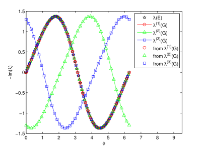
(a) Imaginary part of all eigenvalues computed from matrices $\left\{G_{0},G_{1},\cdots G_{M-1}\right\}$

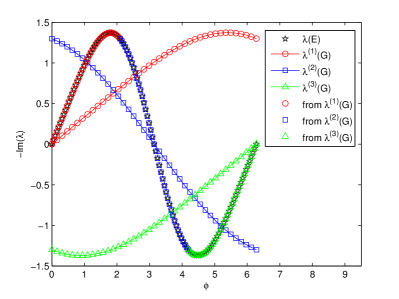
(b) Imaginary part of all eigenvalues computed from matrices $\left\{H_{0},H_{1},\cdots H_{M-1}\right\}$

Figure 24: Imaginary part of eigenvalues computed from two kinds of local matrices for the third-order WCNS, where $z_{1}$, $z_{2}$ and $z_{3}$ are the three eigenvalues of local matrices

Appendix D. Comparisons on spectrum of different high-order schemes

The spectrum of CNNW is compared with WCNS and CPR by computing all eigenvalues from the matrix $G$ with $M=40$.

Fig. 25 shows eigenvalues in the complex plane. we can see that all eigenvalues of each scheme have negative real part, which illustrate that CNNW, CPR and WCNS are stable. In addition, the three groups of eigenvalues (noted by $z1$, $z2$ and $z3$ in the Fig. 25) for third-order schemes are different since $mod(M,3)\neq 0$ and the five groups of eigenvalues for fifth-order schemes are the same since $mod(M,5)=0$. These results agree with Theorem 5.1. Dispersion and dissipation relations in one period are shown for third-order schemes in Fig. 26 and for fifth-order schemes in Fig. 7.

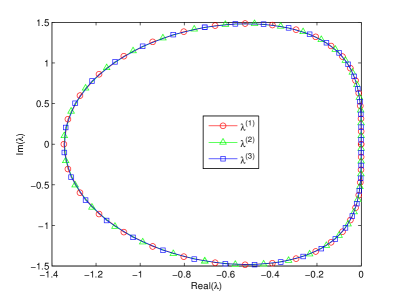
(a) C3NNW3

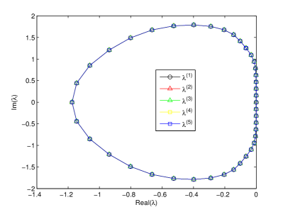
(b) C5NNW5

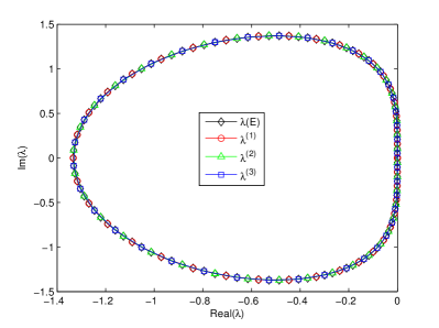
(c) WCNS3

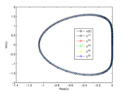
(d) WCNS5

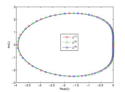
(e) CPR-DG3

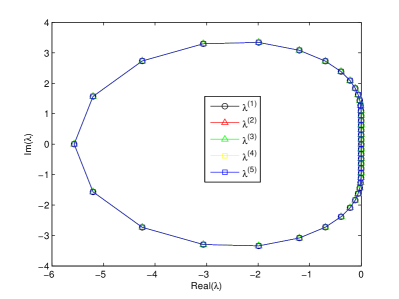
(f) CPR-DG5

Figure 25: Comparison of the eigenvalue spectrum $\left\{\lambda_{m}^{(l)}\left|\lambda_{m}^{(l)}=\lambda^{(l)}(G(\phi_{m})),l=1,2,\cdots K+1;m=0,1,2,\cdots,M\right.\right\}$ where $\phi_{m}=m\frac{2\pi}{M}$ for different high-order schemes ($K=2$ for third-order schemes and $K=4$ for fifth-order schemes) and $M=40$.

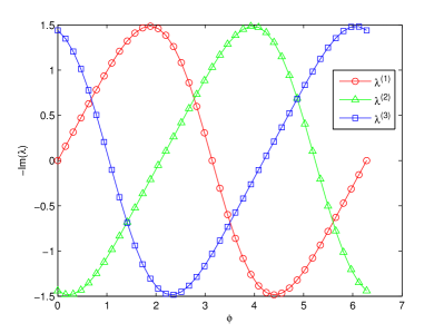
(a) C3NNW3, dispersion

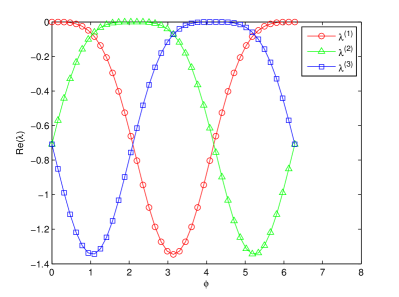
(b) C3NNW3, dissipation

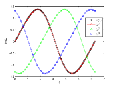
(c) WCNS3, dispersion

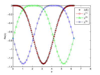
(d) WCNS3, dissipation

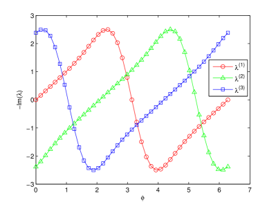
(e) CPR3, dispersion

(f) CPR3, dissipation

Figure 26: Comparison of dispersion (left) and dissipation (right) for third-order schemes, where $\left\{\lambda_{m}^{(l)}\left|\lambda_{m}^{(l)}=\lambda^{(l)}(G(\phi_{m})),l=1,2,\cdots K+1;m=0,1,2,\cdots,M\right.\right\}$, $\phi_{m}=m\frac{2\pi}{M}$, $K=2$ and $M=40$.

Appendix E. NNW2 interpolation

Now we propose second-order nonuniform nonlinear weighted (NNW2) interpolation. Consider the stencil with three nonuniformly spaced solution points $\left\{u_{1},u_{2},u_{3}\right\}$. Take the second solution point for example and set $u_{1}=u_{i,sp_{1}}$, $u_{2}=u_{i,sp_{2}}$, $u_{3}=u_{i,sp_{3}}$, as shown in in Fig. 4. The values at flux points $u_{i,fp_{2}}^{R}$ and $u_{i,fp_{3}}^{L}$, denoted by $u_{A}^{R}$ and $u_{B}^{L}$, can be interpolated from $\left\{u_{1},u_{2},u_{3}\right\}$ by following procedure.

(1) Get $u_{A}^{(1)}$ and $u_{B}^{(1)}$ by inverse distance weighted interpolation,

$$u_{A}^{(1)}=\omega_{1}u_{1}+\omega_{2}u_{2},\quad\omega_{1}=\frac{\left(1/\Delta\xi_{1}\right)}{\left(1/\Delta\xi_{1}\right)+\left(1/\Delta\xi_{2}\right)},\quad\omega_{2}=\frac{\left(1/\Delta\xi_{2}\right)}{\left(1/\Delta\xi_{1}\right)+\left(1/\Delta\xi_{2}\right)};$$

$$u_{B}^{(1)}=\omega_{3}u_{2}+\omega_{4}u_{3},\quad\omega_{3}=\frac{\left(1/\Delta\xi_{3}\right)}{\left(1/\Delta\xi_{3}\right)+\left(1/\Delta\xi_{4}\right)},\quad\omega_{4}=\frac{\left(1/\Delta\xi_{4}\right)}{\left(1/\Delta\xi_{3}\right)+\left(1/\Delta\xi_{4}\right)};$$

where $\Delta\xi_{1}=\xi_{fp2}-\xi_{sp1}$, $\Delta\xi_{2}=\xi_{sp2}-\xi_{fp2}$, $\Delta\xi_{3}=\xi_{fp3}-\xi_{sp2}$, $\Delta\xi_{4}=\xi_{sp3}-\xi_{fp3}$, as shown in Fig. 4.

(2) Calculate the gradient of $\frac{\partial u}{\partial\xi}$ with values $\left\{u_{A}^{(1)},u_{2},u_{B}^{(1)}\right\}$ based on the distances between solution points and flux points, we have

$$\frac{\partial u}{\partial\xi}=\omega_{5}\left(\frac{\partial u}{\partial\xi}\right)^{(1)}+\omega_{6}\left(\frac{\partial u}{\partial\xi}\right)^{(2)},$$ (67)

where

$$\omega_{5}=\frac{\left(1/\Delta\xi_{2}\right)}{\left(1/\Delta\xi_{2}\right)+\left(1/\Delta\xi_{3}\right)},\quad\omega_{6}=\frac{\left(1/\Delta\xi_{3}\right)}{\left(1/\Delta\xi_{2}\right)+\left(1/\Delta\xi_{3}\right)},\quad\left(\frac{\partial u}{\partial\xi}\right)^{(1)}=\frac{u_{2}-u_{A}^{(1)}}{\Delta\xi_{2}},\quad\left(\frac{\partial u}{\partial\xi}\right)^{(2)}=\frac{u_{B}^{(1)}-u_{2}}{\Delta\xi_{3}}.$$

(3) Compute $u_{A}^{(2)}$ and $u_{B}^{(2)}$ based on $u_{2}$ and the gradient $\frac{\partial u}{\partial\xi}$, we obtain

$$u_{A}^{(2)}=u_{2}-\frac{\partial u}{\partial\xi}\Delta\xi_{2},\quad u_{B}^{(2)}=u_{2}+\frac{\partial u}{\partial\xi}\Delta\xi_{3}.$$

(4) Add limiter to control numerical oscillation. $u_{A}^{R}$ and $u_{B}^{L}$ are obtained by linear reconstruction with a limiter,

$$u_{A}^{R} = u_{2}-\phi\frac{\partial u}{\partial\xi}\Delta\xi_{2},\quad u_{B}^{L}=u_{2}+\phi\frac{\partial u}{\partial\xi}\Delta\xi_{3}.$$ (68)

Here we take the following Birth limiter Birth and Jespersen [47]

$$\phi=min\{lim(u_{A}^{(2)}),lim(u_{B}^{(2)})\},$$

where

$$lim(u)= \begin{cases}min\{1,\frac{M-u_{2}}{u-u_{2}}\},&if\,\,u>u_{2},\\ min\{1,\frac{m-u_{2}}{u-u_{2}}\},&if\,\,u<u_{2},\\ 1,&if\,\,u=u_{2},\end{cases}$$

with $m=min\{u_{1},u_{2},u_{3}\}$ and $M=max\{u_{1},u_{2},u_{3}\}$.

References

- Deng et al. [2012] X.G. Deng, M.L. Mao, G.H. Tu, H.X. Zhang, and Y.F. Zhang. High-order and high accurate CFD methods and their applications for complex grid problems. Commun. Comput. Phys., 11:1081–1102, 2012.
- Wang et al. [2013] Z.J. Wang, K. Fidkowski, R. Abgrall, and F. Bassi et al. High-order CFD methods: current status and perspective. Int. J. Numer. Meth. Fluids, 72:811–845, 2013.
- Huynh et al. [2014] H.T. Huynh, Z.J. Wang, and P.E. Vincent. High-order methods for computational fluid dynamics: A brief review of compact differential formulations on unstructured grids. Comput. Fluids, 98:209–220, 2014.
- Wang et al. [2017] Z.J. Wang, Y. Li, F. Jia, G.M. Laskowski, J. Kopriva, U. Paliath, and R. Bhaskaran. Towards industrial large eddy simulation using the FR/CPR method. Comput. Fluids, 156:579–589, 2017.
- Cockburn and Shu [1989] B. Cockburn and C.-W. Shu. TVB Runge-Kutta local projection discontinuous Galerkin finite elementmethod for scalar conservation laws III: one dimensional systems. J. Comput. Phys., 84:90–113, 1989.
- Cockburn and Shu [1998] B. Cockburn and C.-W. Shu. The Runge-Kutta local projection discontinuous Galerkin finite element method for scalar conservation laws V: multidimensional systems. J. Comput. Phys., 141:199–224, 1998.
- Huynh [2007] H. T. Huynh. A flux reconstruction approach to high-order schemes including discontinuous Galerkin methods. In AIAA 2007-4079, 2007.
- Wang and Gao [2009] Z.J. Wang and Haiyang Gao. A unifying lifting collocation penalty formulation including the discontinuous Galerkin, spectral volume/difference methods for conservation laws on mixed grids. J. Comput. Phys., 228:8161–8186, 2009.
- Zhong and Shu [2013] X. Zhong and C.-W. Shu. A simple weighted essentially nonoscillatory limiter for Runge-Kutta discontinuous Galerkin methods. J. Comput. Phys., 232(1):397–415, 2013.
- Vilar [2019] F.O. Vilar. A posteriori correction of high-order discontinuous Galerkin scheme through subcell finite volume formulation and flux reconstruction. J. Comput. Phys., 387:245–279, 2019.
- Persson and Peraire [2006] P.O. Persson and J. Peraire. Subcell shock capturing for discontinuous Galerkin methods. Proceedings of the 44th AIAA Aerospace Science Meeting and Exhibit, 2006.
- Discacciati et al. [2020] N. Discacciati, J.S. Hesthaven, and D. Ray. Cotrolling oscillations in high-order discontinuous Galerkin schemes using artificial viscosity tuned by neural networks. J. Comput. Phys., 409:109304, 2020.
- Yu and Hesthaven [2020] J. Yu and J.S. Hesthaven. A study of several artificial viscosity models within the discontinuous Galerkin framework. Commun. Comput. Phys., 27(5):1309–1343, 2020.
- Feng and Liu [2020] Y.W. Feng and T.G. Liu. A characteristic-featured shock wave indicator on unstructured grids based on training an artificial neuron. J. Comput. Phy., 443:110446, 2020.
- Qiu and Shu [2004] J. Qiu and C.-W. Shu. Hermite WENO schemes and their application as limiters for Runge-Kutta discontinuous Galerkin method: one-dimensional case. J. Comput. Phys., 193:115–135, 2004.
- Balsara et al. [2007] D.S. Balsara, C. Meyer, and M. Dumbser. A sub-cell based indicator for troubled zones in RKDG schemes and a novel class of hybrid RKDG+HWENO schemes. J. Comput. Phys., 226:586–620, 2007.
- Zhu and Qiu [2009] J. Zhu and J.X. Qiu. Hermite WENO schemes and their application as limiters for Runge-Kutta discontinuous Galerkin method iii: Unstructured meshes. J. Sci. Comput., 39(2):293–321, 2009.
- Zhu et al. [2013] J. Zhu, X. Zhong, C.-W. Shu, and J. Qiu. Runge-Kutta discontinuous Galerkin method using a new type of WENO limiters on unstructured meshes. J. Comput. Phys., 248(2):200–220, 2013.
- Du et al. [2015] J. Du, C.-W. Shu, and M.P. Zhang. A simple weighted essentially non-oscillatory limiter for the correction procedure via reconstruction (CPR) framework. Appl. Numer. Math., 95:173–198, 2015.
- Li et al. [2020] W. Li, Q. Wandand, and Y-X. Ren. A p-weighted limiter for the discontinuous Galerkin method on one-dimensional and two-dimensional triangular grids. J. Comput. Phys., 407:109246, 2020.
- Park and Kim [2016] J.S. Park and C. Kim. Hierarchical multi-dimensional limiting strategy for correction procedure via reconstruction. J. Comput. Phy., 308:57–80, 2016.
- Baumann and Oden [1999] C.E. Baumann and J.T. Oden. A discontinuous hp finite element method for the Euler and Navier-Stokes equations. Int. J. Numer. Methods Fluids., 31:79–95, 1999.
- Burbeau et al. [2001] A. Burbeau, P. Sagaut, and C.H. Bruneau. A problem-independent limiter for high-order Runge-Kutta discontinuous Galerkin methods. J. Comput. Phys., 169(1):111–150, 2001.
- Dumbser et al. [2014] M. Dumbser, O. Zanotti, R. Loubere, and S. Diot. A posteriori subcell limiting of the discontinuous Galerkin finite element method for hyperbolic conservation laws. J. Comput. Phys., 278:47–75, 2014.
- Dumbser and Loubere [2016] M. Dumbser and R. Loubere. A simple robust and accurate a posteriori sub-cell finite volume limiter for the discontinuous Galerkin method on unstructured meshes. J. Comput. Phys., 319:163–199, 2016.
- Boscheri and Dumbser [2017] W. Boscheri and M. Dumbser. Arbitrary-Lagrangian-Eulerian discontinuous Galerkin schemes with a posteriori subcell finite volume limiting on moving unstructured meshes. J. Comput. Phys., 346:449–479, 2017.
- Ioriatti and Dumbser [2019] M. Ioriatti and M. Dumbser. A posteriori sub-cell finite volume limiting of staggered semi-implicit discontinuous Galerkin schemes for the shallow water equations. Appl. Numer. Math., 135:443–480, 2019.
- Sonntag and Munz [2017] M. Sonntag and C.D. Munz. Efficient parallelization of a shock capturing for discontinuous Galerkin methods using finite volume sub-cells. J. Sci. Comput., 70(3):1262–1289, 2017.
- Krais et al. [2021] N. Krais, A. Beck, T. Bolemann, and et al. FLEXI: A high order discontinuous Galerkin framework for hyperbolic-parabolic conservation laws. Comput. Math. Appl., 81:186–219, 2021.
- Hennemann et al. [2021] S. Hennemann, A.M. Rueda-Ramírez, F.J. Hindenlang, and G.J. Gassner. A provably entropy stable subcell shock capturing approach for high order split form DG for the compressible Euler equations. J. Comput. Phys., 426:109935, 2021.
- Jiang and Shu [1996] G.S. Jiang and C.-W. Shu. Efficient implementation of weighted ENO schemes. J. Comput. Phys., 126:202–228, 1996.
- Hu and Shu [1999] C. Hu and C.-W. Shu. Weighted essentially non-oscillatory schemes on triangular meshes. J. Comput. Phys., 150:97–127, 1999.
- Shu [2003] C.-W. Shu. High-order finite difference and finite volume WENO schemes and discontinuous Galerkin methods for CFD. Int. J. Comput. Fluid Dynamics, 17:107–118, 2003.
- Shu [2009] C.-W. Shu. High order weighted essentially nonoscillatory schemes for convection dominated problems. SIAM Review, 51(1):82–126, 2009.
- Deng and Zhang [2000] X. Deng and H. Zhang. Developing high-order weighted compact nonlinear schemes. J. Comput. Phys., 165:22–44, 2000.
- Cheng and Liu [2014] J. Cheng and T.G. Liu. A multi-domain hybrid DG and WENO method for hyperbolic conservation laws on hybrid meshes. Commun. Comput. Phys., 16:1116–1134, 2014.
- Zhu et al. [2018] H.J. Zhu, Z.G. Yan, H.Y. Liu, M.L. Mao, and X.G. Deng. High-order hybrid WCNS-CPR schemes on hybrid meshes with curved edges for conservation law I : spatial accuracy and geometric conservation laws. Commun. Comput. Phys., 23(5):1355–1392, 2018.
- Guo et al. [2020] J. Guo, H.J. Zhu, Z.G. Yan, L.Y. Tang, and S.H. Song. High-order hybrid WCNS-CPR scheme for shock capturing of conservation laws. Int. J. Aerospace Eng., page 8825445, 2020.
- Huynh [2009] H. T. Huynh. A reconstruction approach to high-order schemes including discontinuous Galerkin for diffusion. In AIAA 2009-403, 2009.
- Qu et al. [2020] F. Qu, D. Sun, B. Zhou, and J. Bai. Self-similar structures based genuinely two-dimensional Riemann solvers in curvilinear coordinates. J. Comput. Phys., 420:109668, 2020.
- Zhu et al. [2016] H.J. Zhu, X.G. Deng, M.L. Mao, H.Y. Liu, and G.H. Tu. Osher flux with entropy fix for two-dimensional Euler equations. Adv. Appl. Math. Mech., 8(4):670–692, 2016.
- Mengaldo et al. [2016] G. Mengaldo, D. De Grazia, P.E. Vincent, and S.J. Sherwin. On the connections between discontinuous Galerkin and flux reconstruction schemes: Extension to curvilinear meshes. J. Sci. Comput., 67:1272–1292, 2016.
- var Leer [1974] B. var Leer. Towards the ultimate conservative difference scheme II, monotonicity and conservation combined in a second order scheme. J. Comput. Phys., 14:361–370, 1974.
- var Leer [1979] B. var Leer. Towards the ultimate conservative difference scheme V, a second order sequel to Godunov’s method. J. Comput. Phys., 32:101–136, 1979.
- Shi et al. [2002] J. Shi, C.Q. Hu, and C.-W. Shu. A technique of treating negative weights in weno schemes. J. Comput. Phys., 175:108–127, 2002.
- Frink [1991] N. Frink. Upwind scheme for solving the Euler equations on unstructured tetrahedral meshes. AIAA Journal, 30:70–77, 1991.
- Birth and Jespersen [1989] T.J. Birth and D.C. Jespersen. The design and application of upwind schemes on unstructured meshes. AIAA Paper 89-0366, 1989.
- Moura et al. [2015] R.C. Moura, S.J. Sherwin, and J. Peiro. Linear dispersion-diffusion analysis and its application to under-resolved turbulence simulations using discontinuous Galerkin spectral/hp methods. J. Comput. Phys., 298:695–710, 2015.
- Schulz-Rinne [1993] C. Schulz-Rinne. Numerical solution of the Riemann problem for two-dimensional gas dynamics. J. Sci. Comput., 14:1394–1414, 1993.
- Buffard and Clain [2010] T. Buffard and S. Clain. Monoslope and multislope MUSCL methods for unstructured meshes. J. Comput. Phys., 229:3745–3776, 2010.
- Woodward and Colella [1984] P. Woodward and P. Colella. The numerical simulation of two-dimensional fluid flow with strong shocks. J. Comput. Phys., 54:115–173, 1984.
- Rault et al. [2003] A. Rault, G. Chiavassa, and R. Donat. Shock-vortex interactions at high Mach numbers. J. Sci. Comput., 19:347–371, 2003.
- Dumbser and M. Kaser [2007] M. Dumbser and E.F. Toro M. Kaser, V.A. Titarev. Quadrature-free non-oscillatory finite volume schemes on unstructured meshes for nonlinear hyperbolic systems. J. Comput. Phys., 226:204–243, 2007.
- You and Kim [2018] H. You and C. Kim. High-order multi-dimensional limiting strategy with subcell resolution i. two-dimensional mixed meshes. J. Comput. Phy., 375:1005–1032, 2018.
- Borges et al. [2008] R. Borges, M. Carmona, B. Costa, and W. S. Don. An improved weighted essentially non-oscillatory scheme for hyperbolic conservation laws. J. Comput. Phys., 227:3191–3211, 2008.
- Yan et al. [2016] Z.G. Yan, H.Y. Liu, M.L. Mao, H.J. Zhu, and X.G. Deng. New nonlinear weights for improving accuracy and resolution of weighted compact nonlinear scheme. Comput. Fluids, 127:226–240, 2016.
- Davis [1979] P. Davis. Circulant Matrices. Wiley, New York, 1979.
- Li [1988] Q. Li. Eight Lectures on Matrix Theory. Shanghai Science and Technology Press, 1988.