Nucleon-nucleon potentials from $\Delta$-full chiral EFT and implications

Abstract

We closely investigate $NN$ potentials based upon the $\Delta$-full version of chiral effective field theory. We find that recently constructed $NN$ potentials of this kind, which (when applied together with three-nucleon forces) were presented as predicting accurate binding energies and radii for a range of nuclei from $A=16$ to $A=132$ and providing accurate equations of state for nuclear matter, yield a $\chi^{2}$/datum of 60 for the reproduction of the $pp$ data below 100 MeV laboratory energy. This $\chi^{2}$ is more than three times what the Hamada-Johnston potential of the year of 1962 achieved already some 60 years ago. We perceive this historical fact as concerning in view of the current emphasis on precision. We are able to trace the very large $\chi^{2}$ as well as the apparent success of the potentials in nuclear structure to unrealistic predictions for $P$-wave states, in which the $\Delta$-full NNLO potentials are off by up to 40 times the NNLO truncation errors. In fact, we show that, the worse the description of the $P$-wave states, the better the predictions in nuclear structure. Thus, these potentials cannot be seen as the solution to the outstanding problems in current miscroscopic nuclear structure physics.

I Introduction

One of the most fundamental aims in theoretical nuclear physics is to understand nuclear structure and reactions in terms of the basic forces between nucleons. As discussed in numerous review papers ME11 ; EHM09 ; MS16 ; Mac17 ; HKK19 , the nuclear physics community presently perceives chiral effective field theory (EFT) as the authoritative paradigm for the derivation of those forces. This perception is based upon a clearly defined relationship between the fundamental theory of strong interactions, QCD, and chiral EFT via symmetries.

Since a while, it is well established that predictive nuclear structure must include three-nucleon forces (3NFs), besides the usual two-nucleon force (2NF) contribution. The advantage of chiral EFT is that it generates 2NFs and multi-nucleon forces simultaneously and on an equal footing. In the $\Delta$-less theory ME11 , 3NFs occur for the first time at next-to-next-to-leading order (NNLO) and continue to have additional contributions in higher orders. Four-nucleon forces (4NFs) start at next-to-next-to-next-to-leading order (N³LO), but are difficult to implement, which is why they are left out in most present-day calculations. If an explicit $\Delta$-isobar is included in chiral EFT ($\Delta$-full theory ORK94 ; ORK96 ; KGW98 ; KEM07 ), then 3NF contributions start already at next-to-leading order (NLO), which leads to a smoother convergence when advancing from leading order (LO) to NNLO. However, summing up all contributions up to NNLO leads to very similar results for both versions of the theory KEM07 . The convergence of both theories beyond NNLO is expected to be very similar.

In the initial phase, the 3NFs were typically adjusted in $A=3$ and/or the $A=4$ systems and the ab initio calculations were driven up to the oxygen region BNV13 . It turned out that for $A\raisebox{-1.29167pt}{\small$\ \stackrel{{\scriptstyle\textstyle<}}{{\sim}}$ }16$ the ground-state energies and radii are predicted about right, no matter what type of chiral or phenomenological potentials were applied (local, nonlocal, soft, hard, etc.) and what the details of the 3NF adjustments to few-body systems were BNV13 ; Rot11 ; Pia18 ; Lon18 . It may be suggestive to perceive the $\alpha$ substruture of ¹⁶O to be part of the explanation.

The picture changed, when the many-body practitioners were able to move up to medium-mass nuclei (e. g., the calcium or even the tin regions). Large variations of the predictions now occurred depending on what forces were used, and cases of severe underbinding Lon17 as well as of substantial overbinding Bin14 were observed. Ever since the nuclear structure community understands that the ab initio explanation of intermediate and heavy nuclei is a severe, still unsolved, problem.

A seemingly successfull interaction for the intermediate mass region appears to be the force that is commonly denoted by “1.8/2.0(EM)” (sometimes dubbed “the Magic force”) Heb11 ; Heb21 , which is a similarity renormalization group (SRG) evolved version of the N³LO 2NF of Ref. EM03 complemented by a NNLO 3NF adjusted to the triton binding energy and the point charge radius of ⁴He. With this force, the ground-state energies all the way up to the tin isotopes are reproduced perfectly—but with charge radii being on the smaller side Sim17 ; Mor18 . Nuclear matter saturation is also reproduced reasonably well, with a slightly too high saturation density Heb11 . However, these calculations are not consistently ab initio, because the 2NF of “1.8/2.0(EM)” is SRG evolved, while the 3NF is not. Moreover, the SRG evolved 2NF is used like an original force with the induced 3NFs omitted. Still, this force is providing clues for how to get the intermediate and heavy mass region right.

Thus, in the follow-up, there have been attempts to get the medium-mass nuclei under control by means of more consistent ab initio calculations Som20 . Of the various efforts, we will now single out three, which demonstrate in more detail what the problems are.

In Ref. DHS19 , recently developed soft chiral 2NFs EMN17 at NNLO and N³LO were picked up and complemented with 3NFs at NNLO and N³LO, respectively, to fit the triton binding energy and nuclear matter saturation. These forces were then applied in in-medium similarity renormalization group (IM-SRG Her16 ) calculations of finite nuclei up to ⁶⁸Ni predicting underbinding and slightly too large radii Hop19 .

In a separate study Hut20 , the same 2NFs used in Refs. DHS19 ; Hop19 were employed, but with the 3NFs now adjusted to the triton and ¹⁶O ground-state energies. The interactions so obtained reproduce accurately experimental energies and point-proton radii of nuclei up to ⁷⁸Ni Hut20 . However, when the 2NF plus 3NF combinations of Ref. Hut20 are utilized in nuclear matter, then dramatic overbinding and no saturation at reasonable densities is obtained SM20 .

Obviously, there is a problem with achieving simultaneously reasonable results for nuclear matter and medium mass nuclei: In Refs. DHS19 ; Hop19 , nuclear matter is saturated right, but nuclei are underbound; while in Ref. Hut20 , nuclei are bound accurately, but nuclear matter is overbound.

In recent work by the Gőteborg-Oak Ridge (GO) group Eks18 ; Jia20 , the authors present an NNLO model including $\Delta$-isobars that apparently overcomes the above problem. With this model, the authors obtain “accurate binding energies and radii for a range of nuclei from $A=16$ to $A=132$, and provide accurate equations of state for nuclear matter” Jia20 . However, the accuracy of the $NN$ part of these interactions is not checked against $NN$ data. Another aspect of interest (not investigated in Refs. Eks18 ; Jia20 ) is if the inclusion of $\Delta$-degrees of freedom leads to a higher degree of softness. Note that the successful “Magic” 1.8/2.0(EM) potential is very soft since it is SRG evolved. Moreover, a recent study Lu18 , which investigated the essential elements of nuclear binding using nuclear lattice simulations, has come to the conclusion that proper nuclear matter saturation requires a considerable amout of non-locality in the $NN$ interaction implying a high degree of softness.

Thus, there is a need for a deeper understanding of the elements in the recent model by the GO group Eks18 ; Jia20 , and how they come together to produce the reported nuclear structure predictions. To gain this deeper insight, we will investigate the following issues:

1. What are the precision and accuracy of the $\Delta$-full $NN$ potentials developed in Ref. Jia20 ? In the context of chiral EFT, this amounts to asking whether the precision of the $\Delta$-full potentials is consistent with the uncertainty of the chiral order at which they have been derived. And, is the accuracy sufficient for meaningful ab initio predictions? If there are problems with precison and/or accuracy, how does that impact the predictions for nuclear many-body systems?

2. Does the inclusion of $\Delta$-isobars increase the smoothness of the interaction and, if so, how does the $\Delta$ degree of freedom accomplish that?

This paper is organized as follows: In Sec. II, we investigate $NN$ potentials based upon $\Delta$-full chiral EFT which, in Sec. III, are applied in nuclear matter. Our conclusions are summarized in Sec. IV.

II Chiral two-nucleon forces including $\Delta$-isobars

II.1 Definition of $NN$ potentials

We focus on $NN$ potentials at NNLO of the $\Delta$-full theory, which—following the notation introduced in Ref. Jia20 —will be denoted by “$\Delta$NNLO.” The diagrams to consider are displayed in Fig. 1. For illustrative purposes, the figure includes also the graphs that occur at N³LO. The powers that are associated with the various orders are calculated as follows. For a connected diagram of $NN$ scattering, the power is given by ME11

$$\nu=2L+\sum_{i}\delta_{i}\,,$$ (1)

with vertex index

$$\delta_{i}\equiv d_{i}+\frac{f_{i}}{2}-2\,,$$ (2)

where $L$ denotes the number of loops. Moreover, for each vertex $i$, $d_{i}$ is the number of derivatives or pion-mass insertions and $f_{i}$ the number of fermion fields. The sum runs over all vertices $i$ contained in the diagram under consideration.

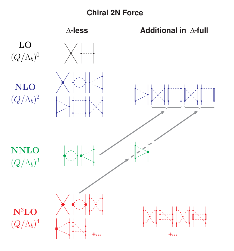
Figure 1: Chiral 2NF without and with $\Delta$-isobar degrees of freedom. Arrows indicate the shift of strength when explicit $\Delta$’s are added to the theory. Note that the $\Delta$-full theory consists of the diagrams involving $\Delta$’s plus the $\Delta$-less ones. Solid lines represent nucleons, double lines $\Delta$-isobars, and dashed lines pions. Small dots, large solid dots, solid squares, and diamonds denote vertices of index $\delta_{i}=\,$ 0, 1, 2, and 4, respectively. $\Lambda_{b}$ denotes the breakdown scale. Further explanations are given in the text.

The mathematical expressions defining the potentials are given in the appendices.

We list the constants involved in the long-range parts of the potentials (cf. Appendix A) in Table 1. These constants have the same values as used in Ref. Jia20 . The $\pi N$ LECs are from the $\pi N$ analysis by Siemens et al. Sie17 , in which the (redundant) subleading $\pi N\Delta$ couplings proportional to $b_{3}$ and $b_{6}$ ($b_{8}$ in the notation of Refs. KEM07 ; FM01 ) are removed by means of a redefinition (renormalization) of the leading order $\pi N\Delta$ axial coupling $h_{A}$ and the subleading $\pi\pi NN$ couplings $c_{i}$ ($i=1,2,3,4$) Sie20 .

The constants that parametrize the short-range parts of the potentials (“$NN$ contact terms,” cf. Appendix B) are shown in Table 2.

Table 1: Hadron masses PDG and pion low-energy constants Sie17 ; Sie20 used throughout this work.

Quantity		Value
Charged-pion mass $m_{\pi^{\pm}}$		139.5702 MeV
Neutral-pion mass $m_{\pi^{0}}$		134.9766 MeV
Average pion-mass $\bar{m}_{\pi}$		138.0390 MeV
Proton mass $M_{p}$		938.2720 MeV
Neutron mass $M_{n}$		939.5654 MeV
Average nucleon-mass $\bar{M}_{N}$		938.9183 MeV
$\Delta$-isobar mass $M_{\Delta}$		1232 MeV
$\Delta\equiv M_{\Delta}-\bar{M}_{N}$		293.0817 MeV
Nucleon axial coupling constant $g_{A}$		1.289
$\pi N\Delta$ axial coupling constant $h_{A}$		1.400
Pion-decay constant $f_{\pi}$		92.2 MeV
$c_{1}$		$-0.74$ GeV-1
$c_{2}$		$-0.49$ GeV-1
$c_{3}$		$-0.65$ GeV-1
$c_{4}$		$+0.96$ GeV-1

Table 2: Partial-wave contact LECs for the $NN$ potentials discussed in this paper. The $\widetilde{C}_{i}$ of the zeroth order partial-wave contact terms defined in Eq. (26) are in units of $10^{4}$ GeV^-2 and the $C_{i}$, Eq. (28), in $10^{4}$ GeV^-4. For SFR and regulator parameters, see Appendix A.2 and C.2, respectively.

LEC	$\Delta$NNLO(450)GO	$\Delta$NNLO(394)GO	$\Delta$NNLO(450)Rf	$\Delta$NNLO(394)Rf
$\widetilde{C}_{{}^{1}S_{0}}^{(pp)}$	–0.339111	–0.338142	–0.326970	–0.327058
$\widetilde{C}_{{}^{1}S_{0}}^{(nn)}$	–0.339887	–0.338746	–0.3274139	–0.32747485
$\widetilde{C}_{{}^{1}S_{0}}^{(np)}$	–0.340114	–0.339250	–0.32778548	–0.32798615
$\widetilde{C}_{{}^{3}S_{1}}$	–0.253950	–0.259839	–0.22116035	–0.23998011
$C_{{}^{1}S_{0}}$	2.526636	2.505389	2.238414	2.180000
$C_{{}^{3}S_{1}}$	0.964990	1.002189	0.760000	0.870000
$C_{{}^{3}S_{1}-^{3}D_{1}}$	0.445743	0.452523	0.370000	0.435000
$C_{{}^{1}P_{1}}$	–0.219498	–0.387960	0.027506	0.027506
$C_{{}^{3}P_{0}}$	0.671908	0.700499	0.858000	0.892000
$C_{{}^{3}P_{1}}$	–0.915398	–0.964856	–0.843000	–0.843000
$C_{{}^{3}P_{2}}$	–0.895405	–0.883122	–0.740000	–0.755000

II.2 Predictions for two-nucleon scattering

We will present the predictions that can be made within the $\Delta$NNLO model in two steps. First, we will show the results obtained by the Gőteborg-Oak Ridge (GO) group. In a second step, we will generate further fits of the $NN$ data within the $\Delta$NNLO model.

II.2.1 Predictions by the GO models

In Ref. Jia20 , the GO group presented two $\Delta$NNLO models, which—following the GO notation—are marked by $\Delta$NNLO(450)_GO and $\Delta$NNLO(394)_GO, where the parenthetical number denotes the value for the cutoff $\Lambda$ in units of MeV used in the regulator function, Eq. (34). Note that all models discussed in this paper share the same ‘basic parameters’ shown in Table 1; the models differ only by the contact term LECs displayed in Table 2 (and SFR and regulator parameters, see Appendix A.2 and C.2, respectively). The LECs listed in columns $\Delta$NNLO(450)_GO and $\Delta$NNLO(394)_GO of Table 2 are from Ref. Jia20 .

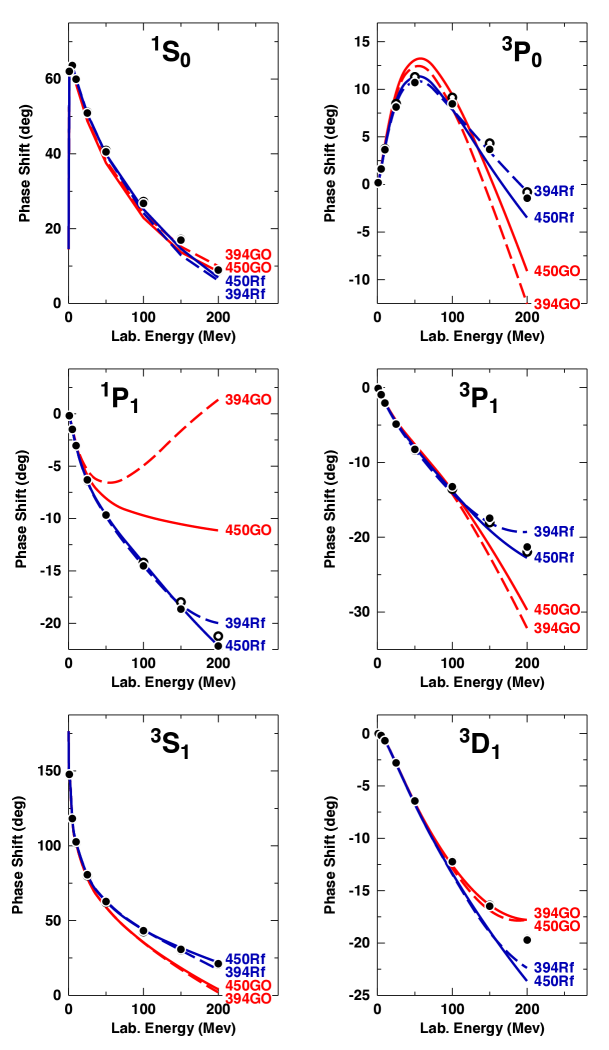
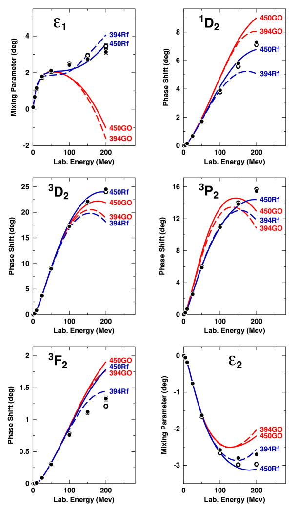
Figure 2: Neutron-proton phase parameters as predicted by the Gőteborg-Oak Ridge (GO) potentials Jia20 [solid red line $\Delta$NNLO(450)_GO, dashed red $\Delta$NNLO(394)_GO] and by our refit (Rf) potentials [solid blue line $\Delta$NNLO(450)_Rf, dashed blue $\Delta$NNLO(394)_Rf]. Partial waves and mixing parameters with total angular momentum $J\leq 2$ are displayed for lab. energies up to 200 MeV. The filled and open circles represent the results from the Nijmegen Sto93 and the Granada PAA13 $np$ phase-shift analyses, respectively.

In Fig. 2, we display the phase parameters for neutron-proton scattering as predicted by the GO models [solid red line $\Delta$NNLO(450)_GO, dashed red $\Delta$NNLO(394)_GO] and compare them with two authoritative phase-shift analyses, namely, the Nijmegen Sto93 and the Granada PAA13 $np$ analyses. It is clearly seen that, above around 100 MeV laboratory energy, the predictions deviate substantially from the analyses in most cases.

Even though it is not uncommon to use phase shifts to provide a qualitative overview, a more precise measure for the accuracy and precision of predictions is obtained from a direct comparison with the $NN$ data. It is customary to state the result of such comparison in terms of the $\chi^{2}$, which is obtained as outlined below.

The experimental data are broken up into groups (sets) of data, $A$, with $N_{A}$ data points and an experimental over-all normalization uncertainty $\Delta n_{A}^{exp}$. For datum $i$, $x^{exp}_{i}$ is the experimental value, $\Delta x^{exp}_{i}$ the experimental uncertainty, and $x^{mod}_{i}$ the model prediction. When fitting the data of group $A$ by a model (or a phase shift solution), the over-all normalization, $n_{A}^{mod}$, is floated and finally chosen such as to minimize the $\chi^{2}$ for this group. The $\chi^{2}$ is then calculated from Ber88

$$\chi^{2}=\sum_{A}\left\{\sum^{N_{A}}_{i=1}\left[\frac{n_{A}^{mod}x^{mod}_{i}-x^{exp}_{i}}{\Delta x^{exp}_{i}}\right]^{2}+\left[\frac{n_{A}^{mod}-1}{\Delta n_{A}^{exp}}\right]^{2}\right\}\;;$$ (3)

that is, the over-all normalization of a group is treated as an additional datum. For groups of data without normalization uncertainty ($\Delta n_{A}^{exp}=0$), $n_{A}^{mod}=1$ is used and the second term on the r.h.s. of Eq. (3) is dropped. The total number of data is

$$N_{dat}=N_{obs}+N_{ne}$$ (4)

where $N_{obs}$ denotes the total number of measured data points (observables), i. e., $N_{obs}=\sum_{A}N_{A}$; and $N_{ne}$ is the number of experimental normalization uncertainties. We state results in terms of $\chi^{2}/N_{dat}\equiv\chi^{2}/$datum, where we use, in general, for the experimental data the 2016 $NN$ base which is defined in Ref. EMN17 .

Table 3: $\chi^{2}/$datum for the reproduction of the $NN$ data by the Gőteborg-Oak Ridge (GO) potentials and by our refit (Rf) potentials. The Hamada-Johnston potential HJ62 is included for comparison.

	Hamada-Johnston
Bin (MeV)	Potential	$\Delta$NNLO(450)GO	$\Delta$NNLO(394)GO	$\Delta$NNLO(450)Rf	$\Delta$NNLO(394)Rf
	of 1962 HJ62 ; foot1 ; SS93
proton-proton
0–100	19.6	60.7	34.3	2.07	1.87
0–200	13.8	46.3	39.7	5.39	10.7
neutron-proton
0–100		5.87	8.58	1.27	1.20
0–200		14.2	26.2	2.23	9.60
$pp$ plus $np$
0–100		28.8	19.3	1.59	1.47
0–200		29.6	32.6	3.71	10.1

In Table 3, we show the $\chi^{2}/$datum for the two Gőteborg-Oak Ridge potentials, $\Delta$NNLO(450)_GO and $\Delta$NNLO(394)_GO, for $pp$ scattering, $np$ scattering, and a combination of both for the lab. energy intervals 0–100 and 0–200 MeV. In the case of the $\Delta$NNLO(450)_GO potential, the over-all $\chi^{2}/$datum for $pp$ plus $np$ is about 30 for all intervals considered, while for $\Delta$NNLO(394)_GO the $\chi^{2}/$datum lies around 20 to 30. The $pp$ $\chi^{2}$ for the interval 0–100 MeV is particularly concerning, because one should expect lower $\chi^{2}$ for lower energies, whereas, in the case of $\Delta$NNLO(450)_GO, the interval of lowest energy has the highest $\chi^{2}$. The reason for this anomaly can be traced to the $P$-wave phase-shifts around 50 MeV (cf. Table 6 and Fig. 4, below) which—as we will demonstrate in Sec. III—have a dramatic impact on nuclear matter predictions. Notice that problems at low energies cannot be well identified from global phase-shift plots (cf. Fig. 2), which corroborates the limited value of phase-shift figures and underscores the importance of the $\chi^{2}$ for the fit of the experimental data.

To put the afore-mentioned $\chi^{2}$ values into perspective, we include in Table 3 the $pp$ $\chi^{2}$ of the first semi-quantitative $NN$ potential constructed in the history of nuclear forces: the Hamada-Johnston potential of 1962 HJ62 . This old-timer yields a $pp$ $\chi^{2}$/datum of 13.8 for the interval 0–183 MeV HJ62 ; foot1 ; SS93 . Thus, the $\chi^{2}$/datum of 46.3 produced by the $\Delta$NNLO(450)_GO potential is more than three times larger than the one of the 60-year-old potential. In fact, none of the historical $NN$ potentials listed in Table II of Ref. SS93 has a $\chi^{2}$ as large as the one of the GO potentials of 2020. Clearly, this is problematic, especially considering that high precision is becoming an increasingly important feature for current advances and goals in ab initio nuclear structure physics INT21 .

In addition to the above historical perspective, it is important to convey some clear physics arguments. Contemporary $NN$ potentials developed within the well-defined framework of an EFT must satisfy specific criteria. The EFT is organized order by order with an appropriate expansion parameter and, consequently, the precision of the predictions can be estimated—being dictated by the truncation error at the order under consideration.

The expansion parameter $Q$ is given by EKM15

$$Q=\max\left\{\frac{m_{\pi}}{\Lambda_{b}},\;\frac{p}{\Lambda_{b}}\right\}\,,$$ (5)

where $p$ is the characteristic center-of-mass (cms) momentum scale and $\Lambda_{b}$ the so-called breakdown scale for which we choose a value of 700 MeV, consistent with the investigations of Ref. Fur15 . The truncation error at NNLO is then determined to be EKM15

$$\Delta X_{\rm NNLO}(p)=\max\left\{Q^{4}\times\left|X_{\rm LO}(p)\right|,\;\;Q^{2}\times\left|X_{\rm LO}(p)-X_{\rm NLO}(p)\right|,\;\;Q\times\left|X_{\rm NLO}(p)-X_{\rm NNLO}(p)\right|\right\}\,,$$ (6)

where $X_{\rm NNLO}(p)$ denotes the NNLO prediction for observable $X(p)$, etc.. Since, in the $\Delta$-full theory, the difference between NLO and NNLO is very small, the third term in the curly bracket is most likely not the maximum. Concerning the remaining two terms, let us start with the first term, $Q^{4}\times\left|X_{\rm LO}(p)\right|$. Assuming that $\left|X_{\rm LO}(p)\right|$ is of the size of the observable under consideration, then $Q^{4}$ represents the (relative) truncation error suggested by the first term. Since $Q$ is momentum dependent, let us consider two energy ranges: A low energy range ($\approx 0-100$ MeV) where $Q=m_{\pi}/\Lambda_{b}=0.2$ and an intermediate energy range ($\approx 100-200$ MeV) around a lab. energy of 150 MeV ($p=265$ MeV/c) implying $Q=p/\Lambda_{b}=0.4$. For these two energy ranges, we have $Q^{4}\approx$ 0.002 and 0.03; or 0.2% and 3%, respectively. When calculating error estimates for the phase shifts shown in Table 6, below, we made the experience that the second term in the curly bracket of Eq. (6), namely the $Q^{2}\times\left|X_{\rm LO}(p)-X_{\rm NLO}(p)\right|$ term , is in general the largest one and as a rule of thumb about twice the $Q^{4}$ term. Therefore, to be on the conservative side, we double the naive estimates and assume truncation errors of 0.4% and 6% for the lab. energy intervals $0-100$ and $100-200$ MeV, respectively.

To make connection with the $\chi^{2}$ formula, Eq. (3), one may identify $\Delta X_{\rm NNLO}(p)\approx\left|(n_{A}^{mod}x^{mod}_{i}-x^{exp}_{i})/x^{exp}_{i}\right|$ for pieces of data $x^{exp}_{i}$ in the energy range characterized by the cms momentum $p$. Thus, to estimate the $\chi^{2}$, one needs an idea of how the truncation error compares to typical experimental errors.

Going over the comprehensive $pp$ data base of Ref. Ber90 reveals that, for low energies, experimental errors around 0.2-0.4% are not uncommon. At intermediate energies, the experimental errors move up to typically 2-4% for the $pp$ as well as the $np$ data Ber90 ; Sto93 . Thus, $\chi^{2}$/datum around 1-2 for low energies and around 2-5 for the higher energy intervall are consistent with the estimated truncation error at NNLO. More compelling evidence is provided by actual calculations. For the $\Delta$-less theory, systematic order-by-order calculations with minimized $\chi^{2}$ have been conducted in Refs. EMN17 ; RKE18 . In the case of the NNLO potential of Ref. EMN17 , $\chi^{2}$/datum of 1.7 and 3.3 are generated for the intervals 0-100 and 0-190 MeV for the combined $np$ plus $pp$ data. These results are in line with our above estimates based upon the truncation error at NNLO, and indicate that a $\chi^{2}$/datum $\approx 30$ is inconsistent with the precision at NNLO.

Low energy scattering parameters and deuteron properties are shown in Table 4 and 5, respectively, which reveal further inaccuracies in the GO potentials.

Some important phase shifts and their NNLO truncation uncertainties are displayed in Table 6, from which one must conclude that the phase shift predictions by the GO potentials are off by 40 times the truncation error in some cases.

Table 4: Scattering lengths ($a$) and effective ranges ($r$) in units of fm as predicted by the Gőteborg-Oak Ridge (GO) potentials and by our refit (Rf) potentials. ($a_{pp}^{C}$ and $r_{pp}^{C}$ refer to the $pp$ parameters in the presence of the Coulomb force. $a^{N}$ and $r^{N}$ denote parameters determined from the nuclear force only and with all electromagnetic effects omitted.)

	$\Delta$NNLO(450)GO	$\Delta$NNLO(394)GO	$\Delta$NNLO(450)Rf	$\Delta$NNLO(394)Rf	Empirical
${}^{1}S_{0}$
$a_{pp}^{C}$	–7.8929	–7.8190	–7.8153	–7.8150	–7.8196(26) Ber88
					–7.8149(29) SES83
$r_{pp}^{C}$	2.870	2.865	2.761	2.732	2.790(14) Ber88
					2.769(14) SES83
$a_{pp}^{N}$	–17.670	–17.377	–17.824	–17.901
$r_{pp}^{N}$	2.953	2.944	2.821	2.791
$a_{nn}^{N}$	–19.382	–18.723	–18.950	–18.950	–18.95(40) Gon06 ; Che08
$r_{nn}^{N}$	2.919	2.916	2.800	2.772	2.75(11) MNS90
$a_{np}$	–23.560	–23.504	–23.738	–23.738	–23.740(20) Mac01
$r_{np}$	2.813	2.797	2.686	2.661	[2.77(5)] Mac01
${}^{3}S_{1}$
$a_{t}$	5.458	5.463	5.422	5.418	5.419(7) Mac01
$r_{t}$	1.820	1.820	1.757	1.751	1.753(8) Mac01

Table 5: Deuteron properties as predicted by the $NN$ potentials of this study. (Binding energy $B_{d}$, asymptotic $S$ state $A_{S}$, asymptotic $D/S$ state $\eta$, structure radius $r_{\rm str}$, quadrupole moment $Q$, $D$-state probability $P_{D}$; the predicted $r_{\rm str}$ and $Q$ are without meson-exchange current contributions and relativistic corrections.)

	$\Delta$NNLO(450)GO	$\Delta$NNLO(394)GO	$\Delta$NNLO(450)Rf	$\Delta$NNLO(394)Rf	Empiricala
$B_{d}$ (MeV)	2.233403	2.227450	2.224575	2.224575	2.224575(9)
$A_{S}$ (fm-1/2)	0.8954	0.8943	0.8856	0.8849	0.8846(9)
$\eta$	0.0253	0.0254	0.0257	0.0256	0.0256(4)
$r_{\rm str}$ (fm)	1.986	1.988	1.969	1.969	1.97507(78)
$Q$ (fm2)	0.268	0.267	0.272	0.267	0.2859(3)
$P_{D}$ (%)	3.12	2.97	4.16	3.49	—

^aSee Table XVIII of Ref. Mac01 for references; the empirical value for $r_{\rm str}$ is from Ref. Jen11 .

II.2.2 Accurate fits for $\Delta$NNLO models

In the next step, we have constructed $\Delta$NNLO models with improved fits—for the purpose of explicitly checking out whether, within the $\Delta$-full theory, we can achieve $\chi^{2}$ that are consistent with the above estimates and the $\chi^{2}$ obtained in Ref. EMN17 for the $\Delta$-less theory. We have dubbed our refits $\Delta$NNLO(450)_Rf and $\Delta$NNLO(394)_Rf (where “Rf” stands for Refit). The parameters of the refits are listed in Table 2 foot3 and the $\chi^{2}$/datum are shown in Table 3. The phase shifts are displayed in Fig. 2 by the blue solid and blue dashed lines. The conclusion is that, within the $\Delta$-full theory, fits can be achieved that are of the same quality as in the $\Delta$-less theory and consistent with the truncation error (cf. also Table 6). In the case of the very soft cutoff of 394 MeV, cutoff artefacts are obviously showing up already below 200 MeV, which is not unexpected.

III Nuclear matter

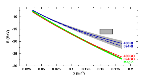
Figure 3: Energy per nucleon in symmetric nuclear matter, $E$, as a function of density, $\rho$, as generated by some two-body forces. Notation for the $\Delta$NNLO potentials as in Fig. 2. Magic (solid green line) refers to the 1.8/2.0(EM) potential of Ref. Heb11 . The shaded band includes the theoretical uncertainties associated with the predictions by the Rf potentials (blue lines) foot2 . Note that this shaded band also covers the predictions by the $\Delta$-less NNLO and N³LO potentials of Ref. EMN17 applied in Ref. Hop19 to intermediate-mass nuclei. The grey box outlines the area where nuclear saturation is expected to occur.

The attempts to explain nuclear matter saturation have a long history Bet71 ; Mac89 . The modern view is that the 3NF is essential to obtain saturation Bog05 ; Heb21 . In this scenario, the 2NF substantially overbinds nuclear matter, while the 3NF contribution is repulsive and strongly density-dependent leading to saturation at the appropriate energy and density Mac19 . Recent example can be found in the work of Ref. DHS19 , where chiral 2NFs at NNLO and N³LO are complemented with chiral 3NFs of the corresponding orders to saturate nuclear matter around its empirical values.

Besides nuclear matter, there is also the problem of the binding energies of intermediate-mass nuclei. When the 2NF+3NF combinations of Ref. DHS19 were applied in IM-SRG calculations of finite nuclei up to the nickel isotops, underbinding of the ground state energies was obtained Hop19 .

On the other hand, also in Ref. Heb11 , 2NF+3NF combinations were developed; in particular, the force known as 1.8/2.0(EM) or Magic, which saturates nuclear matter properly and reproduces the groundstate energies of nuclei up to the tin region correctly Sim17 ; Mor18 .

What is the difference between the two cases?

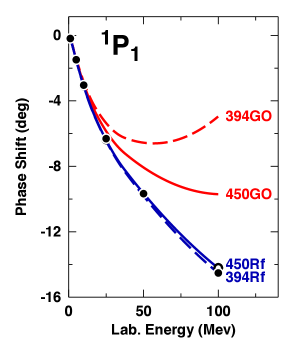
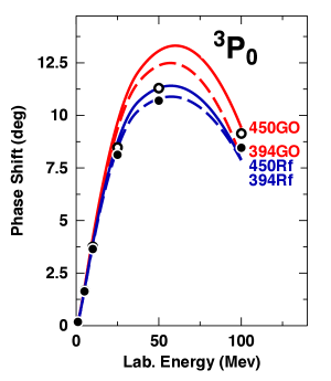
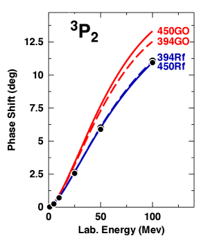
Figure 4: Neutron-proton phase shifts below 100 MeV for three critical $P$-waves. Notation as in Fig. 2.

As it turns out the crucial difference between the two cases is to be found in the 2NF part of the forces. We demonstrate this in Fig. 3, where we show the 2NF contribution to nuclear matter from the 1.8/2.0(EM) force (denoted by Magic, solid green line). On the other hand, the 2NF contribution to nuclear matter from the 2NFs applied in Ref. Hop19 are located within the shaded band in Fig. 3. Even though in both cases nuclear matter is overbound, Magic overbinds considerable more than the NNLO and N³LO forces from Ref. EMN17 applied in Ref. Hop19 to intermediate-mass nuclei. This shows that a considerable overbinding of nuclear matter by the 2NF is necessary to correctly bind intermediate-mass nuclei SM20 , when 3NFs at NNLO are applied.

Next, we turn to the nuclear matter properties as predicted by the $\Delta$-full 2NFs discussed in this paper. We apply the particle-particle ladder approximation [Brueckner-Hartree-Fock (BHF)] for nuclear matter. We have compared our nuclear matter results for the Magic 2NF with the results obtained in Ref. Heb11 where many-body perturbation theory (MBPT) is used and obtain the same within $\pm 0.5$ MeV for all densities displayed in Ref. Heb11 . Moreover, we have also compared our BHF results with the MBPT calculations of Ref. DHS19 (for the $\Lambda=450$ MeV potentials) achieving a similar agreement. From this we conclude that our BHF method for nuclear matter is as reliable as the presently more popular MBPT method for soft potentials.

The predictions by the original GO potentials, $\Delta$NNLO(450)_GO and $\Delta$NNLO(394)_GO, are shown in Fig. 3 by the red solid and dashed curves, respectively. These predictions are right on the Magic curve, which explains the results of the GO potentials for nuclei up to $A=132$ Jia20 , similar to what happens with Magic Sim17 ; Mor18 .

On the other hand, in the previous section we have identified serious problems with the accuracy of the GO $NN$ potentials. For that reason, in Sec. II.2.2 we refitted these potentials, generating the Rf versions $\Delta$NNLO(450)_Rf and $\Delta$NNLO(394)_Rf, which are as accurate as expected at NNLO. The nuclear matter predictions by the Rf potentials are shown by the blue solid and dashed curves in Fig. 3, together with their theoretical uncertainties represented by the shaded band. It is seen that the refitted potentials are less attractive than the original GO versions. In fact, their nuclear matter properties are very similar to the ones of the 2NFs used in Ref. Hop19 and, thus, they will most likely not produce the same results as the original GO potentials and, rather, produce underbinding in intermediate-mass nuclei.

The question we wish to address is then why, after refit to proper accuracy, the $\Delta$NNLO potentials lost attraction. As discussed, the main issues with the GO potentials are found in the $P$-waves at low energy. We demonstrate this in Fig 4, where we show, for the three most important $P$-waves, the phase shifts below 100 MeV as predicted by the original GO potentials (red lines) and and the refit versions in comparison with authoritative phase shift analyses.

Table 6: $np$ phase-parameters, $\delta$ (in degrees), for selected states and laboratory energies, $T_{\rm lab}$, as predicted by the Gőteborg-Oak Ridge (GO) potentials and by our refit (Rf) potentials, for which nuclear matter predictions are shown in Table 7. Empirical values are the averages of the Nijmegen Sto93 and the Granada PAA13 analyses. $\Delta\delta$ is the magnitude of the difference between a prediction and the empirical value. $\Delta\delta_{\rm NNLO}$ denotes the theoretical uncertainty calculated according to Eq. (6) foot2 .

State	$\frac{T_{\rm lab}}{\rm MeV}$	Empirical	$\Delta$NNLO(450)GO		$\Delta$NNLO(394)GO		$\Delta$NNLO(450)Rf		$\Delta$NNLO(394)Rf		$\Delta\delta_{\rm NNLO}$
			$\delta$	$\frac{\Delta\delta}{\Delta\delta_{\rm NNLO}}$	$\delta$	$\frac{\Delta\delta}{\Delta\delta_{\rm NNLO}}$	$\delta$	$\frac{\Delta\delta}{\Delta\delta_{\rm NNLO}}$	$\delta$	$\frac{\Delta\delta}{\Delta\delta_{\rm NNLO}}$
${}^{1}P_{1}$	50	–9.67(5)	–8.07	22.9	–6.56	44.4	–9.65	0.3	–9.81	2.0	0.07
${}^{3}P_{0}$	50	11.00(5)	13.07	2.8	12.37	1.8	11.30	0.4	10.80	0.3	0.75
${}^{3}P_{2}$	50	5.95(1)	7.68	7.5	7.29	5.8	6.01	0.3	6.07	0.5	0.23
${}^{3}S_{1}$	50	62.47 (6)	59.00	9.1	59.00	9.1	62.79	0.9	63.19	1.9	0.38
$\epsilon_{1}$	150	2.84(7)	0.78	5.3	0.59	5.8	2.60	0.6	2.96	0.3	0.39

To further quantify the discrepancies, we provide in Table 6 numerical values for $np$ phase-shifts at 50 MeV lab. energy for the three $P$-waves of interest as predicted by the original GO potentials, the refit potentials, and the phase shift analyses (‘Empirical’). We also provide the NNLO truncation error for the phase shifts, $\Delta\delta_{\rm NNLO}$ foot2 , and state the discrepancies in the fits, $\Delta\delta$, in terms of multiples of the truncation errors, ${\Delta\delta}/{\Delta\delta_{\rm NNLO}}$. For the GO potentials, the discrepancies are on average about ten truncation errors, and can be as large as 44 truncation errors. For the refit potentials, the discrepancies are typically around one truncation error or less – as expected for a properly converging EFT, whose predictions at each order should agree with experiment within the theoretical uncertainty (truncation error) at the given order.

Table 7: Energy contributions per nucleon to symmetric nuclear matter from two-body forces at a density equivalent to a Fermi momentum $k_{F}=1.35$ fm^-1 as obtained in the non-perturbative particle-particle ladder approximation. The Gőteborg-Oak Ridge (GO) $NN$ potentials and our refit (Rf) potentials are applied. Moreover, Magic refers to the 1.8/2.0(EM) $NN$ potential of Ref. Heb11 . $U$ represents the total potential energy per nucleon, $T$ the kinetic energy, and $E$ the total energy per nucleon, $E=T+U$. $U(...)$ denotes the potential energy contribution per nucleon from a particular partial-wave state. All entries are in units of MeV.

	Magic	$\Delta$NNLO(450)GO	$\Delta$NNLO(394)GO	$\Delta$NNLO(450)Rf	$\Delta$NNLO(394)Rf
$U(^{1}P_{1})$	3.71	2.93	2.29	3.71	3.74
$U(^{3}P_{0})$	–3.21	–3.71	–3.56	–3.30	–3.21
$U(^{3}P_{2})$	–7.81	–9.49	–9.15	–7.62	–7.79
$U(^{1}P_{1})+U(^{3}P_{0})+U(^{3}P_{2})$	–7.31	–10.27	–10.42	–7.21	–7.26
$U(^{3}S_{1})$	–27.07	–24.35	–24.61	–22.55	–23.55
$U$	–47.63	–47.11	–47.56	–42.25	–43.11
$T$	22.67	22.67	22.67	22.67	22.67
$E$	–24.96	–24.43	–24.88	–19.57	–20.43

Next, we will explore the impact on nuclear matter from discrepancies in the fit of $NN$ lower partial waves. To investigate this aspect, we show in Table 7 the contributions to the nuclear matter energy around saturation density from distinct partial-wave states. We provide results for the original GO potentials as well as the refit potentials and the Magic potential. Of particular interest are the three $P$-waves that we singled out in Table 6 and Fig. 4. It is seen that, for all three $P$-waves, the contributions from the GO potentials are substatially more attractive than for the other cases. Recalling that, as demonstrated in Fig. 4 and Table 6, all GO potentials overpredict the empirical phase shifts, the increased attraction they generate is not surprising. Thus, while accurately fitted potentials obtain about –7.3 MeV from the three $P$-waves, the GO potentials produce about –10.3 MeV, that is 3 MeV more binding energy per particle. Naturally, this is not a viable source for the additional attraction needed in nuclear structure.

The remaining extra attraction by the GO potentials comes from the ${}^{3}S_{1}$ state, and is on average $\approx 1.5$ MeV as compared to the corresponding Rf potentials. This additional gain in binding energy is, again, linked to unsatisfactory description of phase parameters, in this case the $\epsilon_{1}$ mixing parameter, cf. the $\epsilon_{1}$ frame in Fig. 2. The explantion of this effect is somewhat involved. Note that the $\epsilon_{1}$ parameter is proportional to the strength of the nuclear tensor force. For states in which the tensor force has a dominant role (like the ${}^{3}S_{1}$–${}^{3}D_{1}$–$\epsilon_{1}$ system), the $\widehat{T}$-matrix, Eq. (32), is approximately given by:

$$\widehat{T}({\vec{p}}~{}^{\prime},{\vec{p}})\approx\widehat{V}_{C}({\vec{p}}~{}^{\prime},{\vec{p}})+\int d^{3}p^{\prime\prime}\>\widehat{V}_{T}({\vec{p}}~{}^{\prime},{\vec{p}}~{}^{\prime\prime})\>\frac{M_{N}}{{p}^{2}-{p^{\prime\prime}}^{2}+i\epsilon}\>\widehat{V}_{T}({\vec{p}}~{}^{\prime\prime},{\vec{p}})\,,$$ (7)

where $\widehat{V}_{C}$ denotes the central force and $\widehat{V}_{T}$ the tensor force. The on-shell $\widehat{T}$-matrix is related to the phase-shifts (and observables) of $NN$ scattering. Thus, potentials that fit the same phase shifts produce the same on-shell $\widehat{T}$-matrix elements. However, that does not imply that the potentials are the same. As evident from the above equation, the $\widehat{T}$-matrix is essentially the sum of two terms: the central force term, $\widehat{V}_{C}$, and the second order in $\widehat{V}_{T}$. A potential with a strong $\widehat{V}_{T}$ will produce a large (attractive) second order term and, hence, go along with a weaker (attractive) central force; as compared to a weak tensor force potential, where the lack of attration by the second order term has to be compensated by a stronger (attractive) central force.

Now, when we enter nuclear matter, we encounter particle-particle ladder graphs represented by the $\widehat{G}$-matrix:

$$\widehat{G}({\vec{p}}~{}^{\prime},{\vec{p}})=\widehat{V}({\vec{p}}~{}^{\prime},{\vec{p}})+\int d^{3}p^{\prime\prime}\>\widehat{V}({\vec{p}}~{}^{\prime},{\vec{p}}~{}^{\prime\prime})\>\frac{M_{N}^{\star}\,Q_{P}}{{p}^{2}-{p^{\prime\prime}}^{2}}\>\widehat{G}({\vec{p}}~{}^{\prime\prime},{\vec{p}})\,,$$ (8)

which—similarly to what happened above to the $\widehat{T}$-matrix—for states where the tensor force rules, can be approximated by:

$$\widehat{G}({\vec{p}}~{}^{\prime},{\vec{p}})\approx\widehat{V}_{C}({\vec{p}}~{}^{\prime},{\vec{p}})+\int d^{3}p^{\prime\prime}\>\widehat{V}_{T}({\vec{p}}~{}^{\prime},{\vec{p}}~{}^{\prime\prime})\>\frac{M_{N}^{\star}\,Q_{P}}{{p}^{2}-{p^{\prime\prime}}^{2}}\>\widehat{V}_{T}({\vec{p}}~{}^{\prime\prime},{\vec{p}})\,.$$ (9)

The $\widehat{G}$-matrix equation differs from the $\widehat{T}$-matrix equation in two ways: First, the Pauli projector, $Q_{P}$, which prevents scattering into occupied states and, thus, cuts out the low-momentum spectrum. Second, the single-particle spectrum in nuclear matter, which enhances the energy denominator, thereby decreasing the integrand. Using a simple parametrization of the single particle energies in nuclear matter, this effect comes down to simply replacing the free nucleon mass, $M_{N}$, by the effective mass $M_{N}^{\star}<M_{N}$.

Both medium effects reduce the size of the (attractive) integral term and, thus, are repulsive. The larger $V_{T}$ and the second order $V_{T}$ term, the larger the repulsive effects. Thus, large tensor force potentials undergo a larger reduction of attraction from these medium effects than weak tensor force potentials. This explains the well-known fact that $NN$ potentials with a weaker tensor force yield more attractive results when applied in nuclear few- and many-body systems as compared to their strong tensor force counterparts.

The GO potentials have a very weak tensor force, which explains their relatively large ${}^{3}S_{1}$ contribution (cf. Table 7). In fact, the tensor force is excessively weak, as can be inferred from the underpredicted $\epsilon_{1}$ parameter (cf. Fig. 2). To agree with the empirical information within the truncation error, the tensor force has to be stronger, like in the case of the Rf potentials, leading to less binding energy in nuclear matter.

At this point of our discussion, a word is in place about what laboratory energies of $NN$ scattering are most relevant for predictions in many-body systems. In $P$-waves, about 95% of the contributions to the $\widehat{G}$-matrix, Eq. (8), comes from the Born term. In the sum of the energy contributions from zero to the Fermi-momentum $k_{F}$, the average relative momentum is $\bar{p}=\sqrt{0.3}\,k_{F}$ which, for $k_{F}=1.35$ fm^-1, yields $\bar{p}=146$ MeV/c, equivalent to $T_{\rm lab}=45$ MeV. Thus, for $P$-waves, the phase shifts around $T_{\rm lab}=50$ MeV are most relevant for nuclear matter predictions at saturation density. This fact is particularly evident from the ${}^{3}P_{0}$ phase shifts shown in Fig. 4. In this figure, it is clearly seen that the phase shift predictions around 50 MeV by the GO potentials are substantially too large, meaning too attractive. On the other hand, the ${}^{3}P_{0}$ phase shifts above 100 MeV by the same potentials (cf. Fig. 2) are too low, implying too repulsive. But from Table 7 we know that the GO potentials generate a ${}^{3}P_{0}$ contribution that is too attractive. The conclusion then is that phase shifts below 100 MeV are the most relevant ones for many-body predictions at normal densities – the reason why we chose $T_{\rm lab}=50$ MeV for the discussion of $P$-wave phase shift in Table 6.

The story is different for states where the tensor force plays a dominant role, like in the coupled ${}^{3}S_{1}$–${}^{3}D_{1}$–$\epsilon_{1}$ system, where the integral term in Eq. (9) makes a large contribution. Note that the integration extends from around $k_{F}$ (due to Pauli blocking) to the cutoff region of the potential. Thus, the relative momenta involved are $p\raisebox{-1.29167pt}{\small$\ \stackrel{{\scriptstyle\textstyle>}}{{\sim}}$ }k_{F}$, equivalent to $T_{\rm lab}\raisebox{-1.29167pt}{\small$\ \stackrel{{\scriptstyle\textstyle>}}{{\sim}}$ }150$ MeV for $k_{F}=1.35$ fm^-1, which explains why the $\epsilon_{1}$ mixing parameter needs to be considered for energies of 150 MeV or even higher (cf. Table 6).

Finally, a comment on the many-body predictions by Magic is in order. As seen in Table 7, the $P$-wave contributions from Magic are essentially the same as the ones from the properly fitted Rf potentials, namely –7.31 MeV from the three $P$-waves of special interest. What sets the Magic potential apart from all the others is the exceptionally large ${}^{3}S_{1}$ contribution – note that the $\epsilon_{1}$ predictions by Magic are identical to the ones by the N³LO potential of Ref. EM03 , which are right on the data up 300 MeV. The extraordinarily nonlocal nature of Magic due to its similarity renormalization group (SRG) evolution is the source of the additional attraction that shows up in nuclear structure. This has the consequence that the second order $V_{T}$ term in Eq. (9) is unusually small and, consequently, the central force, $V_{C}$, unusually large and attractive, giving rise to the very large, attractive ${}^{3}S_{1}$ contribution by Magic. This degree of nonlocality can, presently, not be achieved by any original chiral potential, no matter if $\Delta$-full or $\Delta$-less and, therefore, these potentials cannot generate ${}^{3}S_{1}$ contributions as large as the Magic one. Making up for this by incorrect, extra attractive $P$-waves is not a valid solution.

To summarize, when the three $P$-waves and the $\epsilon_{1}$ parameter of the GO potentials are corrected to obtain a realistic fit, the favorable predictions for intermediate-mass nuclei are very likely to disappear, as did the extra attraction in nuclear matter.

IV Conclusions

We have closely investigated chiral $NN$ potentials at NNLO including $\Delta$-isobar degrees of freedom and have come to the following conclusions:

1. The $\Delta$-full $NN$ potentials at NNLO constructed by the Gőteborg-Oak Ridge (GO) group Jia20 are up to 40 times outside the theoretical error of chiral EFT at NNLO and are, therefore, inconsistent with the EFT that the potentials are intended to be based upon. In line with this fact, these potentials reproduce the $NN$ data with a very large $\chi^{2}$. This is unacceptable based on contemporary precision standards.

2. The predictions by the GO $NN$ potentials for the energy per nucleon in nuclear matter are very attractive, similar to the predictions by the 1.8/2.0(EM) $NN$ potential of Ref. Heb11 , also known as ‘Magic’. The extremely attractive nature of both the GO and the Magic potentials is the reason for the favorable reproduction of the energies (and radii) of intermediate-mass nuclei, which have proven to be a problem in ab initio nuclear structure physics. However, the extra attraction in the GO potentials which brings them to the level of Magic can be traced to incorrect $P$-wave and $\epsilon_{1}$ mixing parameters.

3. When all phase parameters, including the $P$-wave and the $\epsilon_{1}$-mixing parameters, are fitted within the NNLO truncation error, then the extra attraction disappears and the nuclear matter predictions become very similar to the ones by $NN$ potentials constructed within the $\Delta$-less theory. Thus, we find claims that $\Delta$-full potentials lead to more attraction in nuclear many-body systems to be incorrect.

4. The extraordinarily attractive nature of Magic is due to its high degree of nonlocality which, in turn, is due to its SRG construction. This degree of nonlocality is not achieved by chiral $NN$ potentials, no matter if $\Delta$s are included or excluded, because all two-pion exchange (2PE) contributions in both version of the theory are local (at least up to NNLO, see appendix) and nonlocality is generated only by the regulator function, which adds only moderate nonlocality.

5. The problem with a microscopic description of intermediate mass nuclei with realistic chiral nuclear forces remains, unfortunately, unsolved.

Appendix A The long-range potential

A.1 Leading order

At leading order, only one-pion exchange (1PE) contributes to the long range. The charge-independent 1PE is given by

$$V_{1\pi}^{\rm(CI)}({\vec{p}}~{}^{\prime},\vec{p})=-\frac{g_{A}^{2}}{4f_{\pi}^{2}}\>\bm{\tau}_{1}\cdot\bm{\tau}_{2}\>\frac{\vec{\sigma}_{1}\cdot\vec{q}\,\,\vec{\sigma}_{2}\cdot\vec{q}}{q^{2}+m_{\pi}^{2}}\,,$$ (10)

where ${\vec{p}}\,^{\prime}$ and $\vec{p}$ denote the final and initial nucleon momenta in the center-of-mass system, respectively. Moreover, $\vec{q}={\vec{p}}\,^{\prime}-\vec{p}$ is the momentum transfer, and $\vec{\sigma}_{1,2}$ and $\bm{\tau}_{1,2}$ are the spin and isospin operators of nucleon 1 and 2, respectively. Parameters $g_{A}$, $f_{\pi}$, and $m_{\pi}$ denote the axial-vector coupling constant, pion-decay constant, and the pion mass, respectively. See Table 1 for their values. Higher order corrections to the 1PE are taken care of by mass and coupling constant renormalizations. Note also that, on shell, there are no relativistic corrections. Thus, we apply 1PE in the form Eq. (10) through all orders.

For the $NN$ potentials considered in this paper, the charge-dependence of the 1PE due to pion-mass splitting is taken into account. Thus, in proton-proton ($pp$) and neutron-neutron ($nn$) scattering, we actually use

$$V_{1\pi}^{(pp)}({\vec{p}}~{}^{\prime},\vec{p})=V_{1\pi}^{(nn)}({\vec{p}}~{}^{\prime},\vec{p})=V_{1\pi}(m_{\pi^{0}})\,,$$ (11)

and in neutron-proton ($np$) scattering, we apply

$$V_{1\pi}^{(np)}({\vec{p}}~{}^{\prime},\vec{p})=-V_{1\pi}(m_{\pi^{0}})+(-1)^{I+1}\,2\,V_{1\pi}(m_{\pi^{\pm}})\,,$$ (12)

where $I=0,1$ denotes the total isospin of the two-nucleon system and

$$V_{1\pi}(m_{\pi})\equiv-\,\frac{g_{A}^{2}}{4f_{\pi}^{2}}\,\frac{\vec{\sigma}_{1}\cdot\vec{q}\,\,\vec{\sigma}_{2}\cdot\vec{q}}{q^{2}+m_{\pi}^{2}}\,,$$ (13)

with the exact values for the various pion masses shown in Table 1.

In this context, we note that, in the 2PE contributions, we neglect the charge-dependence due to pion-mass splitting and apply $m_{\pi}=\bar{m}_{\pi}$ (cf. Table 1).

A.2 Next-to-leading order

We will present the contributions from all subleading pion exchanges in terms of the following template:

$$V({\vec{p}}~{}^{\prime},\vec{p}) = \>\,V_{C}\>\,+\bm{\tau}_{1}\cdot\bm{\tau}_{2}\,W_{C}$$ (14)

$$+ \left[\,V_{S}\>\,+\bm{\tau}_{1}\cdot\bm{\tau}_{2}\,W_{S}\,\>\,\right]\,\vec{\sigma}_{1}\cdot\vec{\sigma}_{2}$$

$$+ \left[\,V_{T}\>\,+\bm{\tau}_{1}\cdot\bm{\tau}_{2}\,W_{T}\,\>\,\right]\,\vec{\sigma}_{1}\cdot\vec{q}\,\,\vec{\sigma}_{2}\cdot\vec{q}\,.$$

Moreover, we regularize the loop contributions from subleading pion exchanges by spectral-function regularization (SFR) EGM04 employing a finite $\tilde{\Lambda}\geq 2m_{\pi}$. The purpose of the finite scale $\tilde{\Lambda}$ is to constrain the loop contributions to the low-momentum region where chiral effective field theory is applicable. Thus, a reasonable choice for $\tilde{\Lambda}$ is to keep it below the masses of the vector mesons $\rho(770)$ and $\omega(782)$, but above the $f_{0}(500)$ [also know as $\sigma(500)$] PDG . This suggests that the region 600-700 MeV is appropriate for $\tilde{\Lambda}$. For the GO potentials Jia20 , $\tilde{\Lambda}=700$ MeV is used, while, following Ref. EMN17 , $\tilde{\Lambda}=650$ MeV is applied for the “Rf” potentials.

A.2.1 $\Delta$-less contributions

The $\Delta$-less $NN$ diagrams that occur at NLO (cf. Fig. 1) contribute in the following way KBW97 :

$$W_{C} = {L(\tilde{\Lambda};q)\over 384\pi^{2}f_{\pi}^{4}}\left[4m_{\pi}^{2}(1+4g_{A}^{2}-5g_{A}^{4})+q^{2}(1+10g_{A}^{2}-23g_{A}^{4})-{48g_{A}^{4}m_{\pi}^{4}\over w^{2}}\right]\,,$$ (15)

$$V_{T} = -{1\over q^{2}}V_{S}\;=\;-{3g_{A}^{4}\over 64\pi^{2}f_{\pi}^{4}}L(\tilde{\Lambda};q)\,,$$ (16)

where the (regularized) logarithmic loop function is given by:

$$L(\tilde{\Lambda};q)={w\over 2q}\ln{\frac{\tilde{\Lambda}^{2}(2m_{\pi}^{2}+q^{2})-2m_{\pi}^{2}q^{2}+\tilde{\Lambda}\sqrt{\tilde{\Lambda}^{2}-4m_{\pi}^{2}}\,q\,w}{2m_{\pi}^{2}(\tilde{\Lambda}^{2}+q^{2})}}$$ (17)

with $w=\sqrt{4m_{\pi}^{2}+q^{2}}$.

A.2.2 $\Delta$-full contributions

The $\Delta$-full diagrams at NLO (cf. Fig. 1) are conveniently subdivided into three groups KGW98 ; KEM07 :

• $\Delta$–excitation in the triangle graph:

  $$W_{C}=-\frac{h_{A}^{2}}{216\pi^{2}f_{\pi}^{4}}\,\left\{(6\Sigma-\omega^{2})L(\tilde{\Lambda};q)+12\Delta^{2}\Sigma D(\tilde{\Lambda};q)\right\}\,;$$ (18)

• single $\Delta$–excitation in the box graphs:

  $$V_{C} = -\frac{g_{A}^{2}\,h_{A}^{2}}{12\pi f_{\pi}^{4}\Delta}\,(2m_{\pi}^{2}+q^{2})^{2}\,A(\tilde{\Lambda};q)\,,$$

  $$W_{C} = -\frac{g_{A}^{2}\,h_{A}^{2}}{216\pi^{2}f_{\pi}^{4}}\,\left\{(12\Delta^{2}-20m_{\pi}^{2}-11q^{2})L(\tilde{\Lambda};q)+6\Sigma^{2}D(\tilde{\Lambda};q)\right\}\,,$$

  $$V_{T} = -\frac{1}{q^{2}}V_{S}=-\frac{g_{A}^{2}\,h_{A}^{2}}{48\pi^{2}f_{\pi}^{4}}\,\left\{-2L(\tilde{\Lambda};q)+(\omega^{2}-4\Delta^{2})D(\tilde{\Lambda};q)\right\}\,,$$

  $$W_{T} = -\frac{1}{q^{2}}W_{S}=-\frac{g_{A}^{2}\,h_{A}^{2}}{144\pi f_{\pi}^{4}\Delta}\,\omega^{2}\,A(\tilde{\Lambda};q)~{};$$ (19)

• double $\Delta$–excitation in the box graphs:

  $$V_{C} = -\frac{h_{A}^{4}}{27\pi^{2}f_{\pi}^{4}}\,\left\{-4\Delta^{2}L(\tilde{\Lambda};q)+\Sigma\left[H(\tilde{\Lambda};q)+(\Sigma+8\Delta^{2})D(\tilde{\Lambda};q)\right]\right\}\,,$$

  $$W_{C} = -\frac{h_{A}^{4}}{486\pi^{2}f_{\pi}^{4}}\,\left\{(12\Sigma-\omega^{2})L(\tilde{\Lambda};q)+3\Sigma\left[H(\tilde{\Lambda};q)+(8\Delta^{2}-\Sigma)D(\tilde{\Lambda};q)\right]\right\}\,,$$

  $$V_{T} = -\frac{1}{q^{2}}V_{S}=-\frac{h_{A}^{4}}{216\pi^{2}f_{\pi}^{4}}\,\left\{6L(\tilde{\Lambda};q)+(12\Delta^{2}-\omega^{2})D(\tilde{\Lambda};q)\right\}\,,$$

  $$W_{T} = -\frac{1}{q^{2}}W_{S}=-\frac{h_{A}^{4}}{1296\pi^{2}f_{\pi}^{4}}\,\left\{2L(\tilde{\Lambda};q)+(4\Delta^{2}+\omega^{2})D(\tilde{\Lambda};q)\right\}\,;$$ (20)

where we are using the following functions:

$$\Sigma = 2m_{\pi}^{2}+q^{2}-2\Delta^{2}\,,$$

$$A(\tilde{\Lambda};q) = {1\over 2q}\arctan{q(\tilde{\Lambda}-2m_{\pi})\over q^{2}+2\tilde{\Lambda}m_{\pi}}\,,$$

$$D(\tilde{\Lambda};q) = \frac{1}{\Delta}\,\int_{2m_{\pi}}^{\tilde{\Lambda}}\frac{d\mu}{\mu^{2}+q^{2}}\,\arctan\frac{\sqrt{\mu^{2}-4m_{\pi}^{2}}}{2\Delta}\,,$$

$$H(\tilde{\Lambda};q) = \frac{2\Sigma}{\omega^{2}-4\Delta^{2}}\left[L(\tilde{\Lambda};q)-L\left(\tilde{\Lambda};2\sqrt{\Delta^{2}-m_{\pi}^{2}}\right)\right]\,;$$ (21)

and $\Delta\equiv M_{\Delta}-\bar{M}_{N}$ the $\Delta$-nucleon mass difference (Table 1). Notice that $\Delta$ is charge-independent to avoid randomly defined charge-dependence.

A.3 Next-to-next-to-leading order

A.3.1 $\Delta$-less contributions

The $\Delta$-less NNLO contribution (cf. Fig. 1) is given by KBW97 :

$$V_{C} = {3g_{A}^{2}\over 16\pi f_{\pi}^{4}}\left[2m_{\pi}^{2}(c_{3}-2c_{1})+c_{3}q^{2}\right](2m_{\pi}^{2}+q^{2})A(\tilde{\Lambda};q)\,,$$ (22)

$$W_{T} = -{1\over q^{2}}W_{S}=-{g_{A}^{2}\over 32\pi f_{\pi}^{4}}c_{4}w^{2}A(\tilde{\Lambda};q)\,.$$ (23)

A.3.2 $\Delta$-full contributions

The subleading triangle diagram with $\Delta$ excitation (cf. Fig. 1) makes the following contribution KEM07 (note that we set $(b_{3}+b_{8})=0$ Sie17 ; Sie20 ):

$$V_{C} = -\frac{h_{A}^{2}\,\Delta}{18\pi^{2}f_{\pi}^{4}}\,\left\{6\Sigma\,\left[4c_{1}m_{\pi}^{2}-2c_{2}\Delta^{2}-c_{3}(2\Delta^{2}+\Sigma)\right]\,D(\tilde{\Lambda};q)\right.$$

$$\left.+\left[-24\,c_{1}m_{\pi}^{2}+c_{2}\,(\omega^{2}-6\Sigma)+6\,c_{3}\,(2\Delta^{2}+\Sigma)\right]L(\tilde{\Lambda};q)\right\}\,,$$

$$W_{T} = -\frac{1}{q^{2}}W_{S}=-\frac{c_{4}\,h_{A}^{2}\,\Delta}{72\pi^{2}f_{\pi}^{4}}\,\left\{(\omega^{2}-4\Delta^{2})D(\tilde{\Lambda};q)-2L(\tilde{\Lambda};q)\right\}\,.$$ (24)

Appendix B The short-range potential

B.1 Zeroth order

The zeroth order (leading order, LO) contact potential is given by

$$V_{\rm ct}^{(0)}(\vec{p^{\prime}},\vec{p})=C_{S}+C_{T}\,\vec{\sigma}_{1}\cdot\vec{\sigma}_{2}\,$$ (25)

and, in terms of partial waves,

$$V_{\rm ct}^{(0)}(^{1}S_{0}) = \widetilde{C}_{{}^{1}S_{0}}=4\pi\,(C_{S}-3\,C_{T})$$

$$V_{\rm ct}^{(0)}(^{3}S_{1}) = \widetilde{C}_{{}^{3}S_{1}}=4\pi\,(C_{S}+C_{T})\,.$$ (26)

To deal with the isospin breaking in the ${}^{1}S_{0}$ state, we treat $\widetilde{C}_{{}^{1}S_{0}}$ in a charge-dependent way. Thus, we will distinguish between $\widetilde{C}_{{}^{1}S_{0}}^{(pp)}$, $\widetilde{C}_{{}^{1}S_{0}}^{(np)}$, and $\widetilde{C}_{{}^{1}S_{0}}^{(nn)}$.

B.2 Second order

At second order (NLO), we have

$$V_{\rm ct}^{(2)}(\vec{p^{\prime}},\vec{p}) = C_{1}\,q^{2}+C_{2}\,k^{2}$$ (27)

$$+ \left(C_{3}\,q^{2}+C_{4}\,k^{2}\right)\vec{\sigma}_{1}\cdot\vec{\sigma}_{2}$$

$$+ C_{5}\left(-i\vec{S}\cdot(\vec{q}\times\vec{k})\right)$$

$$+ C_{6}\,(\vec{\sigma}_{1}\cdot\vec{q})\,(\vec{\sigma}_{2}\cdot\vec{q})$$

$$+ C_{7}\,(\vec{\sigma}_{1}\cdot\vec{k})\,(\vec{\sigma}_{2}\cdot\vec{k})\,,$$

where $\vec{k}=({\vec{p}}\,^{\prime}+\vec{p})/2$ denotes the average momentum and $\vec{S}=(\vec{\sigma}_{1}+\vec{\sigma}_{2})/2$ is the total spin. Partial-wave decomposition yields

$$V_{\rm ct}^{(2)}(^{1}S_{0}) = C_{{}^{1}S_{0}}(p^{2}+{p^{\prime}}^{2})$$

$$V_{\rm ct}^{(2)}(^{3}S_{1}) = C_{{}^{3}S_{1}}(p^{2}+{p^{\prime}}^{2})$$

$$V_{\rm ct}^{(2)}(^{3}S_{1}-^{3}D_{1}) = C_{{}^{3}S_{1}-^{3}D_{1}}p^{2}$$

$$V_{\rm ct}^{(2)}(^{3}D_{1}-^{3}S_{1}) = C_{{}^{3}S_{1}-^{3}D_{1}}{p^{\prime}}^{2}$$

$$V_{\rm ct}^{(2)}(^{1}P_{1}) = C_{{}^{1}P_{1}}\,pp^{\prime}$$

$$V_{\rm ct}^{(2)}(^{3}P_{0}) = C_{{}^{3}P_{0}}\,pp^{\prime}$$

$$V_{\rm ct}^{(2)}(^{3}P_{1}) = C_{{}^{3}P_{1}}\,pp^{\prime}$$

$$V_{\rm ct}^{(2)}(^{3}P_{2}) = C_{{}^{3}P_{2}}\,pp^{\prime}\,.$$ (28)

The relationship between the $C_{{}^{(2S+1)}L_{J}}$ and the $C_{i}$ can be found in Ref. ME11 .

Appendix C Definition of nonrelativistic potential

C.1 Lippmann-Schwinger equation

The potential $V$ is, in principal, an invariant amplitude (with relativity taken into account perturbatively) and, thus, satisfies a relativistic scattering equation, like, e. g., the Blankenbeclar-Sugar (BbS) equation BS66 , which reads explicitly,

$${T}({\vec{p}}~{}^{\prime},{\vec{p}})={V}({\vec{p}}~{}^{\prime},{\vec{p}})+\int\frac{d^{3}p^{\prime\prime}}{(2\pi)^{3}}\>{V}({\vec{p}}~{}^{\prime},{\vec{p}}~{}^{\prime\prime})\>\frac{M_{N}^{2}}{E_{p^{\prime\prime}}}\>\frac{1}{{p}^{2}-{p^{\prime\prime}}^{2}+i\epsilon}\>{T}({\vec{p}}~{}^{\prime\prime},{\vec{p}})$$ (29)

with $E_{p^{\prime\prime}}\equiv\sqrt{M_{N}^{2}+{p^{\prime\prime}}^{2}}$ and $M_{N}$ the nucleon mass. The advantage of using a relativistic scattering equation is that it automatically includes relativistic kinematical corrections to all orders. Thus, in the scattering equation, no propagator modifications are necessary when moving up to higher orders.

Defining

$$\widehat{V}({\vec{p}}~{}^{\prime},{\vec{p}})\equiv\frac{1}{(2\pi)^{3}}\sqrt{\frac{M_{N}}{E_{p^{\prime}}}}\>{V}({\vec{p}}~{}^{\prime},{\vec{p}})\>\sqrt{\frac{M_{N}}{E_{p}}}$$ (30)

and

$$\widehat{T}({\vec{p}}~{}^{\prime},{\vec{p}})\equiv\frac{1}{(2\pi)^{3}}\sqrt{\frac{M_{N}}{E_{p^{\prime}}}}\>{T}({\vec{p}}~{}^{\prime},{\vec{p}})\>\sqrt{\frac{M_{N}}{E_{p}}}\,,$$ (31)

where the factor $1/(2\pi)^{3}$ is added for convenience, the BbS equation collapses into the usual, nonrelativistic Lippmann-Schwinger (LS) equation,

$$\widehat{T}({\vec{p}}~{}^{\prime},{\vec{p}})=\widehat{V}({\vec{p}}~{}^{\prime},{\vec{p}})+\int d^{3}p^{\prime\prime}\>\widehat{V}({\vec{p}}~{}^{\prime},{\vec{p}}~{}^{\prime\prime})\>\frac{M_{N}}{{p}^{2}-{p^{\prime\prime}}^{2}+i\epsilon}\>\widehat{T}({\vec{p}}~{}^{\prime\prime},{\vec{p}})\,.$$ (32)

Since $\widehat{V}$ satisfies Eq. (32), it may be regarded as a nonrelativistic potential. By the same token, $\widehat{T}$ may be considered as the nonrelativistic T-matrix. All technical aspects associated with the solution of the LS equation can be found in Appendix A of Ref. Mac01 , including specific formulas for the calculation of the $np$ and $pp$ phase shifts (with Coulomb). Additional details concerning the relevant operators and their decompositions are given in section 4 of Ref. EAH71 . Finally, computational methods to solve the LS equation are found in Ref. Mac93 .

C.2 Regularization

Iteration of $\widehat{V}$ in the LS equation, Eq. (32), requires cutting $\widehat{V}$ off for high momenta to avoid infinities. This is consistent with the fact that chiral EFT is a low-momentum expansion which is valid only for momenta $Q<\Lambda_{\chi}\approx 1$ GeV. Therefore, the potential $\widehat{V}$ is multiplied with the (nonlocal) regulator function $f(p^{\prime},p)$,

$${\widehat{V}}(\vec{p}~{}^{\prime},{\vec{p}})\longmapsto{\widehat{V}}(\vec{p}~{}^{\prime},{\vec{p}})\,f(p^{\prime},p)$$ (33)

with

$$f(p^{\prime},p)=\exp[-(p^{\prime}/\Lambda)^{2n}-(p/\Lambda)^{2n}]\,.$$ (34)

In this work, $\Lambda$ is either 450 MeV or 394 MeV. The exponent $n$ is to be chosen such that the regulator introduces contributions that are beyond the given order. In the case of the NNLO potentials of this paper where the given order is three, this is guaranteed if, for a contribution of order $\nu$, $n$ is fixed such that $2n+\nu>3$. For the GO potentials Jia20 , $n=3$ is used for $\Lambda=450$ MeV and $n=4$ for $\Lambda=394$ MeV. In the case of the “Rf” potentials, we follow Ref. EMN17 and choose $n=2$ for all contributions, except for $V_{\rm ct}^{(0)}(^{3}S_{1})$, $V_{\rm ct}^{(2)}(^{3}P_{1})$, and $V_{\rm ct}^{(2)}(^{3}P_{2})$ where $n=3,3$, and 2.5, respectively; and $n=4$ for 1PE.

References

- (1) R. Machleidt and D. R. Entem, Phys. Rept. 503, 1-75 (2011).
- (2) E. Epelbaum, H.-W. Hammer, and Ulf-G. Meißner, Rev. Mod. Phys. 81, 1773 (2009).
- (3) R. Machleidt and F. Sammarruca, Physica Scripta 91, 083007 (2016).
- (4) R. Machleidt, Int. J. Mod. Phys. E 26, 1730005 and 1740018 (2017).
- (5) H.-W. Hammer, S. Kőnig, and U. van Kolck, Rev. Mod. Phys. 92, 025004 (2020).
- (6) C. Ordóñez, L. Ray, and U. van Kolck, Phys. Rev. Lett. 72, 1982 (1994).
- (7) C. Ordóñez, L. Ray, and U. van Kolck, Phys. Rev. C 53, 2086 (1996).
- (8) N. Kaiser, S. Gerstendőrfer, and W. Weise, Nucl. Phys. A637, 395 (1998).
- (9) H. Krebs, E. Epelbaum, and U. G. Meissner, Eur. Phys. J. A 32, 127 (2007).
- (10) B. R. Barrett, P. Navratil, and J. P. Vary, Prog. Part. Nucl. Phys. 69, 131-181 (2013).
- (11) R. Roth, J. Langhammer, A. Calci, S. Binder, and P. Navratil, Phys. Rev. Lett. 107, 072501 (2011).
- (12) M. Piarulli, A. Baroni, L. Girlanda, A. Kievsky, A. Lovato, E. Lusk, L. E. Marcucci, S. C. Pieper, R. Schiavilla, M. Viviani, and R. B. Wiringa, Phys. Rev. Lett. 120, 052503 (2018).
- (13) D. Lonardoni, S. Gandolfi, J. E. Lynn, C. Petrie, J. Carlson, K. E. Schmidt, and A. Schwenk, Phys. Rev. C 97, 044318 (2018).
- (14) D. Lonardoni, A. Lovato, S. C. Pieper, and R. B. Wiringa, Phys. Rev. C 96, 024326 (2017).
- (15) S. Binder, J. Langhammer, A. Calci, and R. Roth, Phys. Lett. B 736, 119-123 (2014).
- (16) K. Hebeler, S. K. Bogner, R. J. Furnstahl, A. Nogga and A. Schwenk, Phys. Rev. C 83, 031301 (2011).
- (17) K. Hebeler, Phys. Rept. 890, 1 (2021).
- (18) D. R. Entem and R. Machleidt, Phys. Rev. C 68, 041001 (2003).
- (19) J. Simonis, S. R. Stroberg, K. Hebeler, J. D. Holt, and A. Schwenk, Phys. Rev. C 96, 014303 (2017).
- (20) T. D. Morris, J. Simonis, S. R. Stroberg, C. Stumpf, G. Hagen, J. D. Holt, G. R. Jansen, T. Papenbrock, R. Roth, and A. Schwenk, Phys. Rev. Lett. 120, 152503 (2018).
- (21) V. Somà, P. Navrátil, F. Raimondi, C. Barbieri, and T. Duguet, Phys. Rev. C 101, 014318 (2020).
- (22) C. Drischler, K. Hebeler, and A. Schwenk, Phys. Rev. Lett. 122, 042501 (2019).
- (23) D. R. Entem, R. Machleidt, and Y. Nosyk, Phys. Rev. C 96, no.2, 024004 (2017).
- (24) H. Hergert, S. K. Bogner, T. D. Morris, A. Schwenk, and K. Tsukiyama, Phys. Rept. 621, 165 (2016).
- (25) J. Hoppe, C. Drischler, K. Hebeler, A. Schwenk, and J. Simonis, Phys. Rev. C 100, 024318 (2019).
- (26) T. Hüther, K. Vobig, K. Hebeler, R. Machleidt, and R. Roth, Phys. Lett. B 808, 135651 (2020).
- (27) F. Sammarruca and R. Millerson, Phys. Rev. C 102, 034313 (2020).
- (28) A. Ekström, G. Hagen, T. D. Morris, T. Papenbrock, and P. D. Schwartz, Phys. Rev. C 97, 024332 (2018).
- (29) W. G. Jiang, A. Ekström, C. Forssén, G. Hagen, G. R. Jansen, and T. Papenbrock, Phys. Rev. C 102, 054301 (2020).
- (30) B. N. Lu, N. Li, S. Elhatisari, D. Lee, E. Epelbaum, and U. G. Meißner, Phys. Lett. B 797, 134863 (2019).
- (31) P.A. Zyla et al. (Particle Data Group), Prog. Theor. Exp. Phys. 2020, 083C01 (2020).
- (32) D. Siemens, J. Ruiz de Elvira, E. Epelbaum, M. Hoferichter, H. Krebs, B. Kubis and U. G. Meißner, Phys. Lett. B 770, 27 (2017).
- (33) D. Siemens, “Elastic pion-nucleon scattering in chiral perturbation theory: Explicit (1232) degrees of freedom,” [arXiv:2001.03906 [nucl-th]].
- (34) N. Fettes and U. G. Meissner, Nucl. Phys. A 679, 629-670 (2001).
- (35) V. G. J. Stoks, R. A. M. Klomp, M. C. M. Rentmeester, and J. J. de Swart, Phys. Rev. C 48, 792 (1993).
- (36) R. Navarro Pérez, J. E. Amaro, and E. Ruiz Arriola, Phys. Rev. C 88, 064002 (2013) [erratum: Phys. Rev. C 91, 029901 (2015)].
- (37) J. R. Bergervoet, P. C. van Campen, W. A. van der Sanden, and J. J. de Swart, Phys. Rev. C 38, 15 (1988).
- (38) T. Hamada and I. D. Johnston, Nucl. Phys. 34, 382 (1962).
- (39) The for the Hamada-Johnston potential is from Ref. SS93 . The exact bins are 0–125 and 0–183; and the data base is the Nijmegen one Sto93 .
- (40) Vincent Stoks and J. J. de Swart, Phys. Rev. C 47, 761 (1993).
- (41) See, e.g., workshop entitled Nuclear Forces for Precision Nuclear Physics, Institut for Nuclear Theory, University of Washington, Seattle, Washington, USA, April 19 - May 7, 2021.
- (42) E. Epelbaum, H. Krebs, and U. G. Meißner, Eur. Phys. J. A 51, 53 (2015).
- (43) R. J. Furnstahl, N. Klco, D. R. Phillips, and S. Wesolowski, Phys. Rev. C 92, 024005 (2015).
- (44) J. R. Bergervoet, P. C. van Campen, R. A. M. Klomp, J.-L. de Kok, T. A. Rijken, V. G. J. Stoks, and J. J. de Swart, Phys. Rev. C 41, 1435 (1990).
- (45) P. Reinert, H. Krebs, and E. Epelbaum, Eur. Phys. J. A 54, no.5, 86 (2018).
- (46) W. A. van der Sanden, A. H. Emmen, and J. J. de Swart, Report No. THEF-NYM-83.11, Nijmegen (1983), unpublished; quoted in Ref. Ber88 .
- (47) D. E. González Trotter et al., Phys. Rev. C 73 (2006) 034001.
- (48) Q. Chen et al., Phys. Rev. C 77 (2008) 054002.
- (49) G. A. Miller, M. K. Nefkens, and I. Slaus, Phys. Rep. 194 (1990) 1.
- (50) R. Machleidt, Phys. Rev. C 63, 024001 (2001).
- (51) U. D. Jentschura, A. Matveev, C. G. Parthey, J. Alnis, R. Pohl, Th. Udem, N. Kolachevsky, and T. W. Ha̋nsch, Phys. Rev. A 83, 042505 (2011).
- (52) Columns NNLO(450)Rf and NNLO(394)Rf of Table 2 provide the contact LECs of our refit potentials. Besides this our refit potentials differ slightly from the GO potentials in the choice of the SFR cutoff (cf. preamble of Appendix A.2) and in the choice of the power of the regulator function Eq. (34) (cf. end of Appendix C.2).
- (53) H. A. Bethe, Ann. Rev. Nucl. Part. Sci. 21, 93 (1971).
- (54) R. Machleidt, Adv. Nucl. Phys. 19, 189 (1989).
- (55) S. K. Bogner, A. Schwenk, R. J. Furnstahl, and A. Nogga, Nucl. Phys. A 763, 59 (2005).
- (56) R. Machleidt, “What is wrong with our current nuclear forces,” in: Nuclear Theory in the Supercomputing Era - 2018, eds. A. M. Shirokov and A. I. Mazur (Pacific National University, Khabarovsk, Russia, 2019) p. 21.
- (57) To calculate the NNLO truncation errors, we have constructed LO and -full NLO potentials, besides the NNLO ones, and applied Eq. (6).
- (58) E. Epelbaum, W. Glöckle, and U.-G. Meißner, Eur. Phys. J. A 19, 125 (2004).
- (59) N. Kaiser, R. Brockmann, and W. Weise, Nucl. Phys. A625, 758 (1997).
- (60) R. Blankenbecler and R. Sugar, Phys. Rev. 142, 1051 (1966).
- (61) K. Erkelenz, R. Alzetta, and K. Holinde, Nucl. Phys. A176, 413 (1971).
- (62) R. Machleidt, in: Computational Nuclear Physics 2 – Nuclear Reactions, edited by K. Langanke, J.A. Maruhn, and S.E. Koonin (Springer, New York, 1993) p. 1.