Survey data integration for regression analysis using model calibration

Abstract

We consider regression analysis in the context of data integration. To combine partial information from external sources, we employ the idea of model calibration which introduces a “working” reduced model based on the observed covariates. The working reduced model is not necessarily correctly specified but can be a useful device to incorporate the partial information from the external data. The actual implementation is based on a novel application of the information projection and model calibration weighting. The proposed method is particularly attractive for combining information from several sources with different missing patterns. The proposed method is applied to a real data example combining survey data from Korean National Health and Nutrition Examination Survey and big data from National Health Insurance Sharing Service in Korea.

Key words: Big data; Empirical likelihood; Information projection; Measurement error models; Missing covariates.

1 Introduction

Data integration is an emerging research area in survey sampling. By incorporating the partial information from external samples, one can improve the efficiency of the resulting estimator and obtain a more reliable analysis. Lohr and Raghunathan (2017), Yang and Kim (2020), and Rao (2021) provide reviews of statistical methods of data integration for finite population inference. Many existing methods (e.g., Hidiroglou, 2001; Merkouris, 2010; Zubizarreta, 2015) are mainly concerned with estimating population means or totals while combining information for analytic inference such as regression analysis is not fully explored in the existing literature.

In this paper, we consider regression analysis in the context of data integration. When we combine data sources to perform a combined regression analysis, we may encounter some problems: covariates may not be fully observed or be subject to measurement errors. Thus, one may consider the problem as a missing-covariate regression problem. Robins, Rotnitzky, and Zhao (1994) and Wang, Wang, Zhao, and Ou (1997) discussed semiparametric estimation in regression analysis with missing covariate data under the missing-at-random covariate assumption. In our setup, the external data source with missing covariate can be a census or big data.

Under this setup, Chatterjee, Chen, Maas, and Carroll (2016) developed a data integration method based on the constrained maximum likelihood, which uses a fully parametric model for the likelihood specification and a constraint developed from the reduced model for data integration. The constrained maximum likelihood method is efficient when the model is correctly specified but is not applicable when it is difficult or impossible to specify a correct density function. Kundu, Tang, and Chatterjee (2019) generalized the method of Chatterjee et al. (2016) to consider multiple regression models based on the theory of generalized method of moments (Hansen, 1982, GMM). Recently, Xu and Shao (2020) develop a data integration method using generalized method of moments technique, but their method implicitly assumes that the reduced model is correctly specified. Under a nested case-control design, Shin, Pfeiffer, Graubard, and Gail (2020a) proposed to use the fully observed sample in the phase 2 to fit a parametric model, and missing covariates in the phase 1 sample are imputed; also see Shin, Pfeiffer, Graubard, and Gail (2020b). Zhang, Deng, Wheeler, Qin, and Yu (2021) developed a retrospective empirical likelihood framework to account for sampling bias in case-control studies. Sheng, Sun, Huang, and Kim (2021) develop a penalized empirical likelihood approach to incorporate such information in the logistic regression setup.

To combine partial information from external sources, we employ the idea of model calibration (Wu and Sitter, 2001) which introduces a “working” reduced model based on observed covariates. The model parameters in the reduced model are estimated from the external sources and then combined through a novel application of the empirical likelihood method (Owen, 1991; Qin and Lawless, 1994), which can be viewed as information projection (Csiszár and Shields, 2004). The working reduced model is not necessarily specified correctly, but a good working model can improve the efficiency of the resulting analysis. The proposed method is particularly attractive for combining information from several data sources with different missing patterns. In this case, we only need to specify different working models for different missing patterns.

Besides, our proposed method is based on the first moment conditions like usual regression analyses, so weak assumptions can broaden the applicability of the proposed method to many practical problems. In particular, the proposed method is directly applicable to survey sample data which is the main focus of our paper. We consider a more general regression setup and our proposed empirical likelihood method is different from their empirical likelihood methods and does not require that the working reduced model to be correctly specified.

We highlight the contribution of our paper as follows. First, we propose a unified framework for incorporating external data sources in the regression analysis. The proposed method uses weaker assumptions than the parametric model-based method of Chatterjee et al. (2016) and thus provides more robust estimation results. Second, the proposed method is widely applicable as it can easily handle multiple external data sources as demonstrated in Section 5. It can be also applied to the case where the external data source is subject to selection bias. In the real data application in Section 7, we demonstrated that our proposed method can utilize the external big data with unknown selection probabilities by applying propensity score weighting adjustment. Finally, our proposed method is easy to implement and fully justified theoretically. The computation is simple as it is a direct application of the standard empirical likelihood method and can be easily implemented using the existing software.

The paper is organized as follows. In Section 2, a basic setup is introduced, and the existing methods are presented. Section 3 presents the proposed approach, and Section 4 provides its asymptotic properties. In Section 5, an application to multiple data integration is presented. Section 6 presents simulation studies, followed by the application of the proposed method to real data in Section 7. Some concluding remarks are made in Section 8.

2 Basic Setup

Consider a finite population $\mathcal{U}=\{1,\ldots,N\}$ of size $N$. Associated with the $i$th unit, let $y_{i}$ denote the study variable of interest and $\mbox{\boldmath{$x$}}_{i}=(\mbox{\boldmath{$x$}}_{i1},\mbox{\boldmath{$x$}}_{i2})$ the corresponding auxiliary vector of length $p$. We are interested in estimating a population parameter $\mbox{\boldmath{$\beta$}}_{0}$, which solves $\mbox{\boldmath{$U$}}_{1}(\mbox{\boldmath{$\beta$}})=\sum_{i\in\mathcal{U}}\mbox{\boldmath{$U$}}_{1}(\mbox{\boldmath{$\beta$}};\mbox{\boldmath{$x$}}_{i},y_{i})=\mbox{\boldmath{$0$}}$ where $\mbox{\boldmath{$U$}}_{1}(\mbox{\boldmath{$\beta$}};\mbox{\boldmath{$x$}},y)$ is a pre-specified estimating function for $\beta$. One example of the estimating function is $\mbox{\boldmath{$U$}}_{1}(\mbox{\boldmath{$\beta$}};\mbox{\boldmath{$x$}}_{i},y_{i})=\{y_{i}-m_{1}(\mbox{\boldmath{$x$}}_{i};\mbox{\boldmath{$\beta$}})\}\mbox{\boldmath{$h$}}_{1}(\mbox{\boldmath{$x$}}_{i};\mbox{\boldmath{$\beta$}})$, which is implicitly based on a regression model $E(Y_{i}\mid\mbox{\boldmath{$x$}}_{i})=m_{1}(\mbox{\boldmath{$x$}}_{i};\mbox{\boldmath{$\beta$}})$ on the super-population level for some $\mbox{\boldmath{$h$}}_{1}(\mbox{\boldmath{$x$}}_{i};\mbox{\boldmath{$\beta$}})$ satisfying certain identification conditions (e.g., Kim and Rao, 2009). From the finite population a probability sample $\mathcal{S}_{1}\subset\mathcal{U}$ is selected, and a $Z$-estimator $\hat{\mbox{\boldmath{$\beta$}}}$ can be obtained by solving

$$\hat{\mbox{\boldmath{$U$}}}_{1}(\mbox{\boldmath{$\beta$}})\equiv\sum_{i\in\mathcal{S}_{1}}d_{i}\mbox{\boldmath{$U$}}_{1}(\mbox{\boldmath{$\beta$}};\mbox{\boldmath{$x$}}_{i},y_{i})=\mbox{\boldmath{$0$}},$$ (1)

where $d_{i}$ is the sampling weight for unit $i\in\mathcal{S}_{1}$.

In addition to $\mathcal{S}_{1}$, suppose that we observe $\mbox{\boldmath{$x$}}_{i1}$ and $y_{i}$ throughout the finite population and wish to incorporate this extra information to improve the estimation efficiency of $\hat{\mbox{\boldmath{$\beta$}}}$. Before proposing our method, we introduce two related works, including Chen and Chen (2000) and Chatterjee et al. (2016).

Chen and Chen (2000) first considered this problem in the context of measurement error models. To explain their idea in our setup, we first consider a “working” reduced model,

$$E(Y_{i}\mid\mbox{\boldmath{$x$}}_{i1})=m_{2}(\mbox{\boldmath{$x$}}_{i1};\mbox{\boldmath{$\alpha$}})$$ (2)

for some $\alpha$. Under the working model (2), we can obtain an estimator $\hat{\mbox{\boldmath{$\alpha$}}}$ from the current sample $\mathcal{S}_{1}$ by solving

$$\hat{\mbox{\boldmath{$U$}}}_{2}(\mbox{\boldmath{$\alpha$}})\equiv\sum_{i\in\mathcal{S}_{1}}d_{i}\mbox{\boldmath{$U$}}_{2}({\mbox{\boldmath{$\alpha$}}};\mbox{\boldmath{$x$}}_{i1},y_{i})=\mbox{\boldmath{$0$}},$$ (3)

where $\mbox{\boldmath{$U$}}_{2}({\mbox{\boldmath{$\alpha$}}};\mbox{\boldmath{$x$}}_{i1},y_{i})=\{y_{i}-m_{2}(\mbox{\boldmath{$x$}}_{i1};\mbox{\boldmath{$\alpha$}})\}\mbox{\boldmath{$h$}}_{2}(\mbox{\boldmath{$x$}}_{i1};\mbox{\boldmath{$\alpha$}})$ for some $\mbox{\boldmath{$h$}}_{2}(\mbox{\boldmath{$x$}}_{i1};\mbox{\boldmath{$\alpha$}})$ satisfying conditions similar to ones imposed to $\mbox{\boldmath{$h$}}_{1}(\mbox{\boldmath{$x$}}_{i};\mbox{\boldmath{$\beta$}})$. In addition, one can get ${\mbox{\boldmath{$\alpha$}}}^{*}$ that solves $\sum_{i=1}^{N}\mbox{\boldmath{$U$}}_{2}({\mbox{\boldmath{$\alpha$}}};\mbox{\boldmath{$x$}}_{i1},y_{i})=\mbox{\boldmath{$0$}}$. Chen and Chen (2000) proposed using

$$\hat{\mbox{\boldmath{$\beta$}}}^{*}=\hat{\mbox{\boldmath{$\beta$}}}+\widehat{Cov}(\hat{\mbox{\boldmath{$\beta$}}},\hat{\mbox{\boldmath{$\alpha$}}})\{\hat{V}(\hat{\mbox{\boldmath{$\alpha$}}})\}^{-1}\left({\mbox{\boldmath{$\alpha$}}}^{*}-\hat{\mbox{\boldmath{$\alpha$}}}\right)$$

as an efficient estimator of $\beta$ where $\hat{V}(\cdot)$ and $\widehat{Cov}(\cdot)$ denote the design-based variance and covariance estimators, respectively. The working model in (2) is not necessarily correctly specified, but a good working model can improve the efficiency of the final estimator. While the estimator of Chen and Chen (2000) is theoretically justified, it can be numerically unstable as the estimation errors of the variance and covariance matrix can be large.

Chatterjee et al. (2016) considered a likelihood-based approach using a conditional distribution of $Y_{i}$ given $\mbox{\boldmath{$X$}}_{i}$ with density $f(y_{i}\mid\mbox{\boldmath{$x$}}_{i};\mbox{\boldmath{$\beta$}})$ and imposed a constraint based on external information. Specifically, they proposed to maximize

$$\prod_{i\in\mathcal{S}_{1}}f(y_{i}\mid\mbox{\boldmath{$x$}}_{i};\mbox{\boldmath{$\beta$}})dF(\mbox{\boldmath{$x$}}_{i})$$ (4)

subject to

$$\int\int\mbox{\boldmath{$U$}}_{2}(\mbox{\boldmath{$\alpha$}}^{*};\mbox{\boldmath{$x$}}_{1},y)f(y\mid\mbox{\boldmath{$x$}};\mbox{\boldmath{$\beta$}})dy{dF(\mbox{\boldmath{$x$}})}=\mbox{\boldmath{$0$}},$$ (5)

where $F(\mbox{\boldmath{$x$}})$ is an unspecified distribution function for $x$, $dF(\mbox{\boldmath{$x$}})$ is the Radon-Nikodym derivative of the distribution function $F(\mbox{\boldmath{$x$}})$ with respect to a certain dominating measure, and $\mbox{\boldmath{$\alpha$}}^{*}$ is the model parameter available from an external source. Following the likelihood based approach of Chatterjee et al. (2016), $\mbox{\boldmath{$U$}}_{2}(\mbox{\boldmath{$\alpha$}};\mbox{\boldmath{$x$}}_{i1},y)$ corresponds to the estimating function involving a “reduced” distribution function $g(y_{i}\mid\mbox{\boldmath{$x$}}_{i1};\mbox{\boldmath{$\alpha$}}_{0})$ with model parameter $\mbox{\boldmath{$\alpha$}}_{0}$, where $g(y_{i}\mid\mbox{\boldmath{$x$}}_{i1};\alpha_{0})$ can be incorrectly specified. That is, $\mbox{\boldmath{$\alpha$}}^{*}$ is the external information for $\mbox{\boldmath{$\alpha$}}_{0}$. Chatterjee et al. (2016) estimated $F(\mbox{\boldmath{$x$}})$ nonparametrically by empirical likelihood. By imposing this constraint into the maximum likelihood estimation, the external information $\mbox{\boldmath{$\alpha$}}^{*}$ can be naturally incorporated.

The constrained maximum likelihood (CML) method is not directly applicable to our conditional mean model in (1) as the likelihood function for $\beta$ is not defined in our setup. Besides, the design feature for the probability sample $\mathcal{S}_{1}$ is not directly applicable in their method. Nonetheless, one can use an objective function such as that in generalized method of moments to apply the constrained optimization problem, which is asymptotically equivalent to the empirical likelihood method (Imbens, 2002). The empirical likelihood implementation of CML approach is discussed by Han and Lawless (2019).

3 Proposed Approach

We now consider an alternative approach for combining information from several sources. To combine information from several sources, we use the KL divergence measure to apply the information projection (Csiszár and Shields, 2004) on the model space with constraints. Let ${\hat{P}}$ be the empirical distribution of the sample with

$${\hat{P}}(x,y)=\frac{1}{\sum_{i\in\mathcal{S}_{1}}d_{i}}\sum_{i\in\mathcal{S}_{1}}d_{i}\mathbb{I}\{(x,y)={(x_{i},y_{i})}\}.$$ (6)

Given the empirical distribution $\hat{P}$, we wish to find the minimizer of

$$D({\hat{P}}\parallel{P})=\int\log\{d{\hat{P}}(\mbox{\boldmath{$x$}},y)\}d{\hat{P}}(\mbox{\boldmath{$x$}},y)-\int\log\{d{P}(\mbox{\boldmath{$x$}},y)\}d{\hat{P}}(\mbox{\boldmath{$x$}},y)$$ (7)

with respect to $P$ in the model space. Notice that the first term is a constant and the minimizer of (7) is the pseudo maximum likelihood estimator of $\hat{P}$.

We consider the following constraints in our model at the finite-population level:

$$\sum_{i=1}^{N}\mbox{\boldmath{$U$}}_{1}(\mbox{\boldmath{$\beta$}};\mbox{\boldmath{$x$}}_{i},y_{i})p(\mbox{\boldmath{$x$}}_{i},y_{i})=0\ \mbox{ and }\ \sum_{i=1}^{N}\mbox{\boldmath{$U$}}_{2}(\mbox{\boldmath{$\alpha$}}^{*};\mbox{\boldmath{$x$}}_{i1},y_{i})p(\mbox{\boldmath{$x$}}_{i},y_{i})=0,$$ (8)

where $p(\mbox{\boldmath{$x$}}_{i},y_{i})$ is the point mass assigned to point $(\mbox{\boldmath{$x$}}_{i},y_{i})$ in the finite population satisfying $\sum_{i=1}^{N}p(\mbox{\boldmath{$x$}}_{i},y_{i})=1$. See Figure 1 for a graphical illustration of the information projection.

Figure 1: Information projection for the empirical distribution $\hat{P}$. Note that $P^{*}$ minimizes $D(\hat{P}\parallel P)$ among $P$ satisfying the constraints in (8).

Using the weighted empirical distribution in (6), the KL divergence measure in (7) reduces to $D({\hat{P}}\parallel{P})=\mbox{constant}-\hat{N}^{-1}\sum_{i\in\mathcal{S}_{1}}d_{i}\log\{p(\mbox{\boldmath{$x$}}_{i},y_{i})\}$ where $\hat{N}=\sum_{i\in S_{1}}d_{i}$. Thus, we only have to maximize $l(\mathbf{p})=\sum_{i\in\mathcal{S}_{1}}d_{i}\log(p_{i})$ subject to $\sum_{i=1}^{N}{p_{i}}=1$ and the constraints in (8), where $p_{i}$ abbreviates $p(\mbox{\boldmath{$x$}}_{i},y_{i})$. Note that having $p_{i}>0$ for $i\notin\mathcal{S}_{1}$ will decrease the value of $l(\mathbf{p})=\sum_{i\in\mathcal{S}_{1}}d_{i}\log(p_{i})$, the solution ${\hat{p}_{i}}$ to this optimization problem should give $\hat{p}_{i}=0$ for $i\notin S_{1}$. Therefore, we can safely set $p_{i}=0$ for $i\notin S_{1}$ and express the problem as finding the maximizer of

$$Q(\mbox{\boldmath{$d$}},\mbox{\boldmath{$w$}})=\sum_{i\in\mathcal{S}_{1}}d_{i}\log(w_{i})$$ (9)

subject to

$$\displaystyle\sum_{i\in\mathcal{S}_{1}}w_{i}=1,$$ (10)

$$\displaystyle\sum_{i\in\mathcal{S}_{1}}w_{i}\mbox{\boldmath{$U$}}_{2}({\mbox{\boldmath{$\alpha$}}}^{*};\mbox{\boldmath{$x$}}_{i1},y_{i})=\mbox{\boldmath{$0$}},$$ (11)

$$\displaystyle\sum_{i\in\mathcal{S}_{1}}{w}_{i}\mbox{\boldmath{$U$}}_{1}(\mbox{\boldmath{$\beta$}};\mbox{\boldmath{$x$}}_{i},y_{i})=\mbox{\boldmath{$0$}}.$$

We use $w_{i}$ instead of $p_{i}$ to represent the final weights assigned to the sample elements.

Remark 1.

Maximizing the objective function in (9) is equivalent to minimizing the following cross entropy:

$$-\sum_{i\in\mathcal{S}_{1}}\tilde{d}_{i}\log(w_{i}),$$ (12)

where $\tilde{d}_{i}=d_{i}/(\sum_{i\in\mathcal{S}_{1}}d_{i})$. The objective function (12) is also the pseudo empirical log-likelihood function considered by Chen and Sitter (1999) and Wu and Rao (2006). Instead of (9), we may consider other objective functions, including the population empirical likelihood proposed by Chen and Kim (2014) for example.

Our proposed method is different from Chatterjee et al. (2016) in that we use a more general integral constraint (5) which does not involve the conditional density function $f(y\mid\mbox{\boldmath{$x$}};\mbox{\boldmath{$\beta$}})$. Constraint (11) still incorporates the extra information in $\mbox{\boldmath{$\alpha$}}^{*}$. The above optimization can be solved by applying the standard profile empirical likelihood method or using the following two-step estimation method.

1. Find the calibration weights $\hat{\mbox{\boldmath{$w$}}}=\{\hat{w}_{i}:i\in\mathcal{S}_{1}\}$ maximizing $Q(\mbox{\boldmath{$d$}},\mbox{\boldmath{$w$}})$ subject to (10)–(11).

2. Once the solution $\hat{\mbox{\boldmath{$w$}}}$ is obtained from the calibration, estimate $\beta$ by solving

   $$\sum_{i\in\mathcal{S}_{1}}\hat{w}_{i}\mbox{\boldmath{$U$}}_{1}(\mbox{\boldmath{$\beta$}};\mbox{\boldmath{$x$}}_{i},y_{i})=\mbox{\boldmath{$0$}}.$$ (13)

If the benchmark $\mbox{\boldmath{$\alpha$}}^{*}$ is not available from the finite population but can be estimated from an independent external sample, we can use the information from both the original internal sample and the external sample to obtain the benchmark estimate. In practical situations, we may not have access to the raw data of the external sample but often be able to have its summary statistics. Suppose that the external sample provides a point estimator $\hat{\mbox{\boldmath{$\alpha$}}}_{2}$ and its variance estimator $\mbox{\boldmath{$V$}}_{2}=\hat{V}(\hat{\mbox{\boldmath{$\alpha$}}}_{2})$ for the working reduced model in (2). Then, an estimator of the benchmark $\mbox{\boldmath{$\alpha$}}^{*}$ can be obtained by

$$\hat{\mbox{\boldmath{$\alpha$}}}^{*}=(\mbox{\boldmath{$V$}}_{1}^{-1}+\mbox{\boldmath{$V$}}_{2}^{-1})^{-1}(\mbox{\boldmath{$V$}}_{1}^{-1}\hat{\mbox{\boldmath{$\alpha$}}}_{1}+\mbox{\boldmath{$V$}}_{2}^{-1}\hat{\mbox{\boldmath{$\alpha$}}}_{2})$$ (14)

where $\hat{\mbox{\boldmath{$\alpha$}}}_{1}$ and $\mbox{\boldmath{$V$}}_{1}$ are estimated with the internal sample $\mathcal{S}_{1}$. Once $\hat{\mbox{\boldmath{$\alpha$}}}^{*}$ is obtained by (14), it replaces $\mbox{\boldmath{$\alpha$}}^{*}$ in the calibration equation in (11).

Similarly to Wu and Sitter (2001), the proposed method does not require a “true” working model as explained below. Let $\hat{\mbox{\boldmath{$U$}}}_{\text{ext}}(\mbox{\boldmath{$\alpha$}})=0$ be the estimating equation for obtaining $\mbox{\boldmath{$\alpha$}}^{*}$ computed from the external sample $\mathcal{S}_{2}$. Now, the final estimating function for $\beta$ using the model calibration $\hat{\mbox{\boldmath{$U$}}}_{\text{cal}}(\mbox{\boldmath{$\beta$}})=\sum_{i\in\mathcal{S}_{1}}\hat{w}_{i}{\mbox{\boldmath{$U$}}}_{1}(\mbox{\boldmath{$\beta$}};\mbox{\boldmath{$x$}}_{i},y_{i})$ can be approximated by

$$\hat{\mbox{\boldmath{$U$}}}_{\text{cal}}(\mbox{\boldmath{$\beta$}})\doteq\hat{\mbox{\boldmath{$U$}}}_{1}(\mbox{\boldmath{$\beta$}})+\mbox{\boldmath{$K$}}\left\{\hat{\mbox{\boldmath{$U$}}}_{\text{ext}}(\mbox{\boldmath{$\alpha$}}^{*})-\hat{\mbox{\boldmath{$U$}}}_{2}(\mbox{\boldmath{$\alpha$}}^{*})\right\}$$ (15)

for some $K$ where $\hat{\mbox{\boldmath{$U$}}}_{1}(\mbox{\boldmath{$\beta$}})$ and $\hat{\mbox{\boldmath{$U$}}}_{2}(\mbox{\boldmath{$\alpha$}})$ are computed by (1) and (3), respectively, from the internal sample $\mathcal{S}_{1}$. The approximation in (15) can be easily derived using the asymptotic equivalence of the calibration estimator and the regression estimator. Thus, even if $E\{\hat{\mbox{\boldmath{$U$}}}_{\text{ext}}(\mbox{\boldmath{$\alpha$}}^{*})\}$ is not equal to zero, the solution to $\hat{\mbox{\boldmath{$U$}}}_{\text{cal}}(\mbox{\boldmath{$\beta$}})=0$ is consistent as $E\{\hat{\mbox{\boldmath{$U$}}}_{\text{ext}}(\mbox{\boldmath{$\alpha$}})-\hat{\mbox{\boldmath{$U$}}}_{2}(\mbox{\boldmath{$\alpha$}})\}=0$ by design.

Remark 2.

Although the working model $E(Y_{i}\mid\mbox{\boldmath{$x$}}_{i1})=m_{2}(\mbox{\boldmath{$x$}}_{i1};\mbox{\boldmath{$\alpha$}})$ does not need to be correctly specified, we can systematically find $\mbox{\boldmath{$U$}}_{2}(\mbox{\boldmath{$\alpha$}};\mbox{\boldmath{$x$}}_{i1},y_{i})$ by casting its construction as a missing covariate problem, relying on the regression calibration technique. For example, suppose that $\mbox{\boldmath{$x$}}_{i}=(x_{i1},x_{i2})$, we set a predictor $\hat{x}_{i2}={\beta}_{0}+{\beta}_{1}x_{i1}$, and an estimating equation is written by

$$\mbox{\boldmath{$U$}}_{1}(\mbox{\boldmath{$\beta$}};x_{i1},\hat{x}_{i2},y_{i})=\left\{y_{i}-m_{1}(x_{i1},\hat{x}_{i2};\mbox{\boldmath{$\beta$}})\right\}\mbox{\boldmath{$h$}}_{1}(x_{i1},\hat{x}_{i2};\mbox{\boldmath{$\beta$}})$$ (16)

for the control function of the model calibration method where $\mbox{\boldmath{$\beta$}}=(\beta_{0},\beta_{1})$. We can either estimate $\beta$ from sample $\mathcal{S}_{1}$ or use any fixed parameter value as long as the solution to $\sum_{i\in\mathcal{S}_{1}}d_{i}\mbox{\boldmath{$U$}}_{1}(\mbox{\boldmath{$\beta$}};x_{i1},\hat{x}_{i2},y_{i})=\mbox{\boldmath{$0$}}$ is unique. A benchmark estimator of $\beta$ can be obtained using external samples to apply the proposed model calibration method. If we use the control function in (16), then we are essentially treating a regression of $y$ on $x_{1}$ and $\hat{x}_{2}$ as the “working” model for model calibration. This is feasible only when we have direct access to an external sample $\mathcal{S}_{2}$ in addition to the internal sample $\mathcal{S}_{1}$.

4 Theoretical properties

In this section, we investigate the asymptotic properties of the the proposed estimator $\hat{\mbox{\boldmath{$\beta$}}}$ to (13). Since the population parameters including $\mbox{\boldmath{$\beta$}}_{0}$ and $\mbox{\boldmath{$\alpha$}}^{*}$ are determined by the finite population of size $N$, we explicitly use subscript $N$ for those in this section, e.g., $\mbox{\boldmath{$\beta$}}_{0N}$ and $\mbox{\boldmath{$\alpha$}}_{N}^{*}$, but we omit this subscript for $(d_{i},\mbox{\boldmath{$x$}}_{i},y_{i})$ for simplicity. We consider two scenarios: when $\mbox{\boldmath{$\alpha$}}_{N}^{*}$ is available from the finite population and when we only have an external sample to estimate $\mbox{\boldmath{$\alpha$}}_{N}^{*}$ by the generalized least square in (14).

4.1 $\mbox{\boldmath{$\alpha$}}_{N}^{*}$ is available

Let $\tilde{d}_{i}=\hat{N}^{-1}d_{i}$ where $\hat{N}=\sum_{i\in\mathcal{S}_{1}}d_{i}$ is the Horvitz–Thompson estimator of the population size $N$. Replacing $d_{i}$ by $\tilde{d}_{i}$ in (9), we consider the Lagrangian problem that maximizes

$$l(\mbox{\boldmath{$w$}},\mbox{\boldmath{$\lambda$}},\phi)=\sum_{i\in\mathcal{S}_{1}}\tilde{d}_{i}\log(w_{i})+\mbox{\boldmath{$\lambda$}}^{\top}\sum_{i\in\mathcal{S}_{1}}w_{i}\mbox{\boldmath{$U$}}_{2}(\mbox{\boldmath{$\alpha$}}_{N}^{*};\mbox{\boldmath{$x$}}_{i1},y_{i})+\phi\left(\sum_{i\in\mathcal{S}_{1}}w_{i}-1\right)$$

where $\lambda$ and $\phi$ are the Lagrange multipliers.

By setting $\partial l(\mbox{\boldmath{$w$}},\mbox{\boldmath{$\lambda$}},\phi)/\partial\mbox{\boldmath{$\lambda$}}=\mbox{\boldmath{$0$}}$, $\partial l(\mbox{\boldmath{$w$}},\mbox{\boldmath{$\lambda$}},\phi)/\partial\phi=0$ and $\partial l(\mbox{\boldmath{$w$}},\mbox{\boldmath{$\lambda$}},\phi)/\partial w_{i}=0$ for $i\in\mathcal{S}_{1}$, we get $\hat{\phi}=-1$ and $\hat{w}_{i}=\tilde{d}_{i}\{1-\mbox{\boldmath{$\lambda$}}^{\top}\mbox{\boldmath{$U$}}_{2}(\mbox{\boldmath{$\alpha$}}_{N}^{*};\mbox{\boldmath{$x$}}_{i1},y_{i})\}^{-1}$. Then, the proposed method is equivalent to solving $g(\mbox{\boldmath{$\beta$}},\mbox{\boldmath{$\lambda$}})=\mbox{\boldmath{$0$}}$ where

$$g(\mbox{\boldmath{$\beta$}},\mbox{\boldmath{$\lambda$}})=\begin{pmatrix}\displaystyle\sum_{i\in\mathcal{S}_{1}}\frac{\tilde{d}_{i}}{1-\mbox{\boldmath{$\lambda$}}^{\top}\mbox{\boldmath{$U$}}_{2}(\mbox{\boldmath{$\alpha$}}_{N}^{*};\mbox{\boldmath{$x$}}_{i1},y_{i})}\mbox{\boldmath{$U$}}_{1}(\mbox{\boldmath{$\beta$}};\mbox{\boldmath{$x$}}_{i},y_{i})\\ \displaystyle\sum_{i\in\mathcal{S}_{1}}\frac{\tilde{d}_{i}}{1-\mbox{\boldmath{$\lambda$}}^{\top}\mbox{\boldmath{$U$}}_{2}(\mbox{\boldmath{$\alpha$}}_{N}^{*};\mbox{\boldmath{$x$}}_{i1},y_{i})}\mbox{\boldmath{$U$}}_{2}(\mbox{\boldmath{$\alpha$}}_{N}^{*};\mbox{\boldmath{$x$}}_{i1},y_{i})\end{pmatrix}.$$ (17)

Denote the solution to (17) as $\hat{\mbox{\boldmath{$\eta$}}}=(\hat{\mbox{\boldmath{$\beta$}}}{}^{\top},\hat{\mbox{\boldmath{$\lambda$}}}{}^{\top}){}^{\top}$. To investigate asymptotic properties of $\hat{\mbox{\boldmath{$\eta$}}}$, we propose the following regularity conditions.

1. There exists a compact set $\mathcal{A}$ such that $Z_{S}=\sup_{\boldsymbol{\alpha}\in\mathcal{A}}\max_{i\in\mathcal{S}_{1}}\lVert\mbox{\boldmath{$U$}}_{2}(\mbox{\boldmath{$\alpha$}};\mbox{\boldmath{$x$}}_{i1},y_{i})\rVert=o_{p}(n^{1/2})$ and $\mbox{\boldmath{$\alpha$}}_{N}^{*}\in\mathcal{A}$ for $N\in\mathbb{N}$ where $\lVert\cdot\rVert$ denotes the Euclidean norm and the stochastic order is with respect to the sampling design.

2. The sampling design satisfies the following convergence results.

   1. There exist a compact set $\Omega$ such that $\mbox{\boldmath{$\beta$}}_{0N}\in\Omega$ for $N\in\mathbb{N}$ and an interior point of $\Omega$, $\mbox{\boldmath{$\beta$}}_{p}$, such that $\lim_{N\to\infty}\mbox{\boldmath{$\beta$}}_{0N}=\mbox{\boldmath{$\beta$}}_{p}$.

   2. There exists a continuous function $\mbox{\boldmath{$U$}}_{0}(\mbox{\boldmath{$\beta$}})$ over $\Omega$ such that $\sup_{\boldsymbol{\beta}\in\Omega}\lVert\sum_{i\in\mathcal{S}_{1}}\tilde{d}_{i}\mbox{\boldmath{$U$}}_{1}(\mbox{\boldmath{$\beta$}};\mbox{\boldmath{$x$}}_{i},y_{i})-\mbox{\boldmath{$U$}}_{0}(\mbox{\boldmath{$\beta$}})\rVert\to 0$ in probability where $\mbox{\boldmath{$\beta$}}_{p}$ is the unique solution to $\mbox{\boldmath{$U$}}_{0}(\mbox{\boldmath{$\beta$}})=\mbox{\boldmath{$0$}}$.

   3. $\sum_{i\in\mathcal{S}_{1}}\tilde{d}_{i}\partial\mbox{\boldmath{$U$}}_{1}(\mbox{\boldmath{$\beta$}}_{0N};\mbox{\boldmath{$x$}}_{i},y_{i})/\partial\mbox{\boldmath{$\beta$}}^{\top}=\boldsymbol{\mathcal{I}}_{11}+o_{p}(1)$ where $\boldsymbol{\mathcal{I}}_{11}$ is non-stochastic and invertible.

   4. $\sum_{i\in\mathcal{S}_{1}}\tilde{d}_{i}\mbox{\boldmath{$U$}}_{1}(\mbox{\boldmath{$\beta$}}_{0N};\mbox{\boldmath{$x$}}_{i},y_{i})\mbox{\boldmath{$U$}}_{2}(\mbox{\boldmath{$\alpha$}}_{N}^{*};\mbox{\boldmath{$x$}}_{i1},y_{i}){}^{\top}=\boldsymbol{\mathcal{I}}_{12}+o_{p}(1)$ where $\boldsymbol{\mathcal{I}}_{12}$ is non-stochastic.

   5. $\sum_{i\in\mathcal{S}_{1}}\tilde{d}_{i}\mbox{\boldmath{$U$}}_{2}(\mbox{\boldmath{$\alpha$}}_{N}^{*};\mbox{\boldmath{$x$}}_{i1},y_{i})^{\otimes 2}=\boldsymbol{\mathcal{I}}_{22}+o_{p}(1)$ where $\mbox{\boldmath{$A$}}^{\otimes 2}=\mbox{\boldmath{$A$}}\mbox{\boldmath{$A$}}^{\top}$ for any matrix $A$ and $\boldsymbol{\mathcal{I}}_{22}$ is non-stochastic and positively definitive.

3. The sampling design satisfies

   $$n^{1/2}\sum_{i\in\mathcal{S}_{1}}\tilde{d}_{i}\begin{pmatrix}\mbox{\boldmath{$U$}}_{1}(\mbox{\boldmath{$\beta$}}_{0N};\mbox{\boldmath{$x$}}_{i},y_{i})\\ \mbox{\boldmath{$U$}}_{2}(\mbox{\boldmath{$\alpha$}}_{N}^{*};\mbox{\boldmath{$x$}}_{i1},y_{i})\end{pmatrix}\to\mathcal{N}(\mbox{\boldmath{$0$}},\mbox{\boldmath{$\Sigma$}}_{u})$$

   in distribution where $\mathcal{N}(\mbox{\boldmath{$0$}},\mbox{\boldmath{$\Sigma$}}_{u})$ is a normal distribution with mean zero and covariance matrix

   $$\mbox{\boldmath{$\Sigma$}}_{u}=\begin{pmatrix}\mbox{\boldmath{$\Sigma$}}_{11}&\mbox{\boldmath{$\Sigma$}}_{12}\\ \mbox{\boldmath{$\Sigma$}}_{21}&\mbox{\boldmath{$\Sigma$}}_{22}\end{pmatrix}.$$

C1 is a technical condition to obtain the asymptotic order of $\hat{\mbox{\boldmath{$\lambda$}}}$, and a similar condition is also assumed by Wu and Rao (2006); see their condition C1 for details. C2 assumes several convergence results for the two estimating functions. Specifically, C2a shows the parameter space of the finite population parameter $\mbox{\boldmath{$\beta$}}_{0N}$, and the convergence of $\mbox{\boldmath{$\beta$}}_{0N}$ can be satisfied under regularity conditions. Condition C2b is necessary to show $\hat{\mbox{\boldmath{$\beta$}}}-\mbox{\boldmath{$\beta$}}_{p}\to 0$ in probability, then $\hat{\mbox{\boldmath{$\beta$}}}-\mbox{\boldmath{$\beta$}}_{0N}\to 0$ in probability, coupled with C2a. Conditions C2c–C2e guarantee the central limit theorem for $\hat{\mbox{\boldmath{$\eta$}}}$. Note that $\boldsymbol{\mathcal{I}}_{22}$ is symmetric by C2e, but $\boldsymbol{\mathcal{I}}_{11}$ in C2c may be asymmetric for a certain estimating function $\mbox{\boldmath{$U$}}_{1}(\mbox{\boldmath{$\beta$}};\mbox{\boldmath{$x$}},y)$. Condition C3 is satisfied under regularity conditions for general sampling designs; see Fuller (2009, Section 1.3) for details.

Theorem 1.

Suppose that conditions C1–C3 hold. Then, $n^{1/2}(\hat{\mbox{\boldmath{$\eta$}}}-\mbox{\boldmath{$\eta$}}_{0})\to\mathcal{N}(\mbox{\boldmath{$0$}},\mbox{\boldmath{$\Sigma$}}_{\eta})$ in distribution where $\mbox{\boldmath{$\Sigma$}}_{\eta}=\boldsymbol{\mathcal{I}}^{-1}\mbox{\boldmath{$\Sigma$}}_{u}(\boldsymbol{\mathcal{I}}^{-1})^{\top}$ and

$$\boldsymbol{\mathcal{I}}=\begin{pmatrix}\boldsymbol{\mathcal{I}}_{11}&\boldsymbol{\mathcal{I}}_{12}\\ \mbox{\boldmath{$0$}}&\boldsymbol{\mathcal{I}}_{22}\end{pmatrix}.$$

The proof of Theorem 1 is presented in Appendix A. By Theorem 1, we can obtain that $n^{1/2}(\hat{\mbox{\boldmath{$\beta$}}}-\mbox{\boldmath{$\beta$}}_{0N})\to\mathcal{N}(\mbox{\boldmath{$0$}},\mbox{\boldmath{$\Sigma$}}_{\beta})$ in distribution where

$$\mbox{\boldmath{$\Sigma$}}_{\beta}=\boldsymbol{\mathcal{I}}_{11}^{-1}\mbox{\boldmath{$\Sigma$}}_{11}(\boldsymbol{\mathcal{I}}_{11}^{-1})^{{\mathrm{\scriptscriptstyle T}}}-\boldsymbol{\mathcal{I}}_{11}^{-1}\boldsymbol{\mathcal{I}}_{12}\boldsymbol{\mathcal{I}}_{22}^{-1}\mbox{\boldmath{$\Sigma$}}_{21}(\boldsymbol{\mathcal{I}}_{11}^{-1})^{{\mathrm{\scriptscriptstyle T}}}-\boldsymbol{\mathcal{I}}_{11}^{-1}\mbox{\boldmath{$\Sigma$}}_{12}\boldsymbol{\mathcal{I}}_{22}^{-1}\boldsymbol{\mathcal{I}}_{12}^{{\mathrm{\scriptscriptstyle T}}}(\boldsymbol{\mathcal{I}}_{11}^{-1})^{{\mathrm{\scriptscriptstyle T}}}+\boldsymbol{\mathcal{I}}_{11}^{-1}\boldsymbol{\mathcal{I}}_{12}\boldsymbol{\mathcal{I}}_{22}^{-1}\mbox{\boldmath{$\Sigma$}}_{22}\boldsymbol{\mathcal{I}}_{22}^{-1}\boldsymbol{\mathcal{I}}_{12}^{{\mathrm{\scriptscriptstyle T}}}(\boldsymbol{\mathcal{I}}_{11}^{-1})^{{\mathrm{\scriptscriptstyle T}}}$$

and $\mbox{\boldmath{$\Sigma$}}_{11}$ and $\mbox{\boldmath{$\Sigma$}}_{22}$ correspond to the asymptotic variances of $n^{1/2}\sum_{i\in\mathcal{S}_{1}}\tilde{d}_{i}\mbox{\boldmath{$U$}}_{1}(\mbox{\boldmath{$\beta$}}_{0N};\mbox{\boldmath{$x$}}_{i},y_{i})$ and $n^{1/2}\sum_{i\in\mathcal{S}_{1}}\tilde{d}_{i}\mbox{\boldmath{$U$}}_{2}(\mbox{\boldmath{$\alpha$}}_{N}^{*};\mbox{\boldmath{$x$}}_{i1},y_{i})$, respectively. Furthermore, we have the following result regarding the optimality of $\mbox{\boldmath{$U$}}_{2}(\mbox{\boldmath{$\alpha$}}_{N}^{*};\mbox{\boldmath{$x$}}_{i1},y_{i})$.

Corollary 1.

Suppose that the conditions in Theorem 1 hold. For a fixed estimating function $\mbox{\boldmath{$U$}}_{1}(\mbox{\boldmath{$\beta$}};\mbox{\boldmath{$x$}},y)$, $\hat{\mbox{\boldmath{$\beta$}}}$ is optimal if $\boldsymbol{\mathcal{I}}_{12}\boldsymbol{\mathcal{I}}_{22}^{-1}\mbox{\boldmath{$U$}}_{2}(\mbox{\boldmath{$\alpha$}}_{N}^{*};\mbox{\boldmath{$x$}}_{1},y)=E\{\mbox{\boldmath{$U$}}_{1}(\mbox{\boldmath{$\beta$}}_{0N};\mbox{\boldmath{$x$}},y)\mid\mbox{\boldmath{$x$}}_{1},y\}$ holds almost surely for the working reduced model, where $\mbox{\boldmath{$x$}}=(\mbox{\boldmath{$x$}}_{1},\mbox{\boldmath{$x$}}_{2})$, and the expectation is taken with respect to the super-population model.

The proof of Corollary 1 is relegated to Appendix B. Corollary 1 presents a sufficient condition on the reduced model to guarantee an optimal estimator $\hat{\mbox{\boldmath{$\beta$}}}$ if the working model is correctly specified. That is, even if we do not require that the reduced model is correctly specified for consistency, the efficiency gain is guaranteed only under the correct model specification. By Corollary 1, an optimal estimator of $\mbox{\boldmath{$\alpha$}}_{N}^{*}$ can be obtained by solving $E\{\mbox{\boldmath{$U$}}_{1}(\mbox{\boldmath{$\beta$}}_{0N};\mbox{\boldmath{$x$}},y)\mid\mbox{\boldmath{$x$}}_{1},y\}=\mbox{\boldmath{$0$}}$.

Under regularity conditions, it can be shown that $\mbox{\boldmath{$\Sigma$}}_{\beta}=\boldsymbol{\mathcal{I}}_{11}^{-1}(\mbox{\boldmath{$\Sigma$}}_{11}-\mbox{\boldmath{$\Sigma$}}_{12}\mbox{\boldmath{$\Sigma$}}_{22}^{-1}\mbox{\boldmath{$\Sigma$}}_{21})(\boldsymbol{\mathcal{I}}_{11}^{-1})^{\top}$ for simple random sampling with or without replacement. Since $\boldsymbol{\mathcal{I}}_{11}^{-1}\mbox{\boldmath{$\Sigma$}}_{11}(\boldsymbol{\mathcal{I}}_{11}^{-1})^{\top}$ is the asymptotic variance of $n^{1/2}(\hat{\mbox{\boldmath{$\beta$}}}_{m}-\mbox{\boldmath{$\beta$}}_{0N})$ where $\hat{\mbox{\boldmath{$\beta$}}}_{m}$ solves $\sum_{i\in\mathcal{S}_{1}}d_{i}\mbox{\boldmath{$U$}}_{1}(\mbox{\boldmath{$\beta$}};\mbox{\boldmath{$x$}}_{i},y_{i})=0$, the proposed approach achieves efficient estimation under simple random sampling; see S1 of the Supplementary Material for details.

4.2 An external estimator $\hat{\mbox{\boldmath{$\alpha$}}}_{2}$ is available

When $\mbox{\boldmath{$\alpha$}}^{*}$ is not available but an external sample is available to get $\hat{\mbox{\boldmath{$\alpha$}}}^{*}$ in (14), we consider

$$\tilde{g}(\mbox{\boldmath{$\eta$}})=\begin{pmatrix}\displaystyle\sum_{i\in\mathcal{S}_{1}}\frac{\tilde{d}_{i}}{1-\mbox{\boldmath{$\lambda$}}^{\top}\mbox{\boldmath{$U$}}_{2}(\hat{\mbox{\boldmath{$\alpha$}}}^{*};\mbox{\boldmath{$x$}}_{i1},y_{i})}\mbox{\boldmath{$U$}}_{1}(\mbox{\boldmath{$\beta$}};\mbox{\boldmath{$x$}}_{i},y_{i})\\ \displaystyle\sum_{i\in\mathcal{S}_{1}}\frac{\tilde{d}_{i}}{1-\mbox{\boldmath{$\lambda$}}^{\top}\mbox{\boldmath{$U$}}_{2}(\hat{\mbox{\boldmath{$\alpha$}}}^{*};\mbox{\boldmath{$x$}}_{i1},y_{i})}\mbox{\boldmath{$U$}}_{2}(\hat{\mbox{\boldmath{$\alpha$}}}^{*};\mbox{\boldmath{$x$}}_{i1},y_{i})\par\end{pmatrix}.$$ (18)

Denote $\tilde{\mbox{\boldmath{$\eta$}}}$ to be the solution of $\tilde{g}(\mbox{\boldmath{$\eta$}})=\mbox{\boldmath{$0$}}$. Then, the following additional assumptions are required to get the asymptotic properties for $\tilde{\mbox{\boldmath{$\eta$}}}$.

1. $\sum_{i\in\mathcal{S}_{1}}\tilde{d}_{i}\partial\mbox{\boldmath{$U$}}_{2}(\mbox{\boldmath{$\alpha$}};\mbox{\boldmath{$x$}}_{i1},y_{i})/\partial\mbox{\boldmath{$\alpha$}}^{\top}=\boldsymbol{\mathcal{I}}(\mbox{\boldmath{$\alpha$}})+o_{p}(1)$ uniformly for $\mbox{\boldmath{$\alpha$}}\in\mathcal{A}$ where $\boldsymbol{\mathcal{I}}(\mbox{\boldmath{$\alpha$}})$ is non-stochastic. Besides, there exists an invertible matrix $\boldsymbol{\mathcal{I}}_{0}$ such that $\lim_{N\to\infty}\boldsymbol{\mathcal{I}}(\mbox{\boldmath{$\alpha$}}_{N}^{*})=\boldsymbol{\mathcal{I}}_{0}$.

2. The sampling design and the external sample satisfy the following convergence results.

   1. Both $\hat{\mbox{\boldmath{$\alpha$}}}_{1}$ and $\hat{\mbox{\boldmath{$\alpha$}}}_{2}$ are consistent for $\mbox{\boldmath{$\alpha$}}^{*}$.

   2. $\mbox{\boldmath{$V$}}_{1}$ and $\mbox{\boldmath{$V$}}_{2}$ are design consistent variance estimators of $\hat{\mbox{\boldmath{$\alpha$}}}_{1}$ and $\hat{\mbox{\boldmath{$\alpha$}}}_{2}$, respectively.

   3. $\mbox{\boldmath{$V$}}_{1}^{-1}$, $\mbox{\boldmath{$V$}}_{2}^{-1}$, and $(\mbox{\boldmath{$V$}}_{1}^{-1}+\mbox{\boldmath{$V$}}_{2}^{-1})^{-1}$ exist in probability.

   4. $(\mbox{\boldmath{$V$}}_{1}^{-1}+\mbox{\boldmath{$V$}}_{2}^{-1})^{-1}\mbox{\boldmath{$V$}}_{2}^{-1}=\mbox{\boldmath{$W$}}+o_{p}(1)$ where $W$ is non-stochastic.

   5. There exists a scaling function $\gamma(n)$ such that $\gamma(n)(\hat{\mbox{\boldmath{$\alpha$}}}_{2}-\mbox{\boldmath{$\alpha$}}^{*})\to\mathcal{N}(0,\mbox{\boldmath{$\Sigma$}}_{2})$ in distribution where $\mbox{\boldmath{$\Sigma$}}_{2}$ satisfies $\gamma(n)^{2}\mbox{\boldmath{$V$}}_{2}=\mbox{\boldmath{$\Sigma$}}_{2}+o_{p}(1)$.

C4 is used to obtain the asymptotic order and the variance of $\hat{\mbox{\boldmath{$\alpha$}}}^{*}-\mbox{\boldmath{$\alpha$}}_{N}^{*}$, and a similar condition was used by Yuan and Jennrich (1998). C5a and C5b assume the consistency of $\hat{\mbox{\boldmath{$\alpha$}}}_{2}$ and $\mbox{\boldmath{$V$}}_{2}$ obtained by an external sample. For the consistency of $\hat{\mbox{\boldmath{$\alpha$}}}_{1}$, a sufficient condition is similar with C2b. The design consistency of the variance estimator $\mbox{\boldmath{$V$}}_{1}$ can be obtained under general sampling designs; see Fuller (2009, Chapter 1) for details. C5c guarantees the existence of $\hat{\mbox{\boldmath{$\alpha$}}}^{*}$ for the proposed method. C5e shows the central limit theorem with respect to the summary statistic $\hat{\mbox{\boldmath{$\alpha$}}}_{2}$, and it is used to derive a similar result as C3 with $\mbox{\boldmath{$\alpha$}}^{*}$ replaced by $\hat{\mbox{\boldmath{$\alpha$}}}^{*}$. Specifically, the convergence rate of $(\hat{\mbox{\boldmath{$\alpha$}}}_{2}-\mbox{\boldmath{$\alpha$}}^{*})$ is $\gamma(n)^{-1}$, which is determined by the external sample.

The following theorem establishes an asymptotic distribution similar to that in C3.

Theorem 2.

Suppose that conditions C1 and C3–C5 hold. Then,

$$n^{1/2}\sum_{i\in\mathcal{S}_{1}}\tilde{d}_{i}\begin{pmatrix}\mbox{\boldmath{$U$}}_{1}(\mbox{\boldmath{$\beta$}}_{0};\mbox{\boldmath{$x$}}_{i},y_{i})\\ \mbox{\boldmath{$U$}}_{2}(\hat{\mbox{\boldmath{$\alpha$}}}^{*};\mbox{\boldmath{$x$}}_{i1},y_{i})\end{pmatrix}\to\mathcal{N}(\mbox{\boldmath{$0$}},\tilde{\mbox{\boldmath{$\Sigma$}}}_{u})$$

in distribution where

$$\tilde{\mbox{\boldmath{$\Sigma$}}}_{u}=\begin{pmatrix}\tilde{\mbox{\boldmath{$\Sigma$}}}_{11}&\tilde{\mbox{\boldmath{$\Sigma$}}}_{12}\\ \tilde{\mbox{\boldmath{$\Sigma$}}}_{21}&\tilde{\mbox{\boldmath{$\Sigma$}}}_{22}\end{pmatrix}$$

Case 1. Specifically, if there exists a non-stochastic matrix $\mbox{\boldmath{$\Sigma$}}_{c}$ such that $n\mbox{\boldmath{$V$}}_{2}=\mbox{\boldmath{$\Sigma$}}_{c}+o_{p}(1)$, then $\tilde{\mbox{\boldmath{$\Sigma$}}}_{11}=\mbox{\boldmath{$\Sigma$}}_{11}$, $\tilde{\mbox{\boldmath{$\Sigma$}}}_{12}=\mbox{\boldmath{$\Sigma$}}_{12}(\boldsymbol{\mathcal{I}}_{0}^{-1})^{\top}\mbox{\boldmath{$W$}}^{\top}\boldsymbol{\mathcal{I}}_{0}^{\top}$, $\tilde{\mbox{\boldmath{$\Sigma$}}}_{21}=\tilde{\mbox{\boldmath{$\Sigma$}}}_{12}^{{\mathrm{\scriptscriptstyle T}}}$ and $\tilde{\mbox{\boldmath{$\Sigma$}}}_{22}=\boldsymbol{\mathcal{I}}_{0}\mbox{\boldmath{$W$}}\{\mbox{\boldmath{$\Sigma$}}_{c}+\boldsymbol{\mathcal{I}}_{0}^{-1}\mbox{\boldmath{$\Sigma$}}_{22}(\boldsymbol{\mathcal{I}}_{0}^{-1})^{{\mathrm{\scriptscriptstyle T}}}\}\mbox{\boldmath{$W$}}^{{\mathrm{\scriptscriptstyle T}}}\boldsymbol{\mathcal{I}}_{o}^{{\mathrm{\scriptscriptstyle T}}}$;

Case 2. If $\mbox{\boldmath{$W$}}=0$, then $\tilde{\mbox{\boldmath{$\Sigma$}}}_{ij}=\mbox{\boldmath{$0$}}$ for $(i,j)\neq(1,1)$ and $\tilde{\mbox{\boldmath{$\Sigma$}}}_{11}=\mbox{\boldmath{$\Sigma$}}_{11}$.

The proof of Theorem 2 is presented in Appendix C. For Case 1, if $\hat{\mbox{\boldmath{$\alpha$}}}_{2}$ estimated from an external sample is much more efficient than $\hat{\mbox{\boldmath{$\alpha$}}}$ in the sense of $(\hat{\mbox{\boldmath{$\alpha$}}}_{2}-\mbox{\boldmath{$\alpha$}}_{N}^{*})=o_{p}(n^{-1/2})$, then $W$ is an identity matrix and $\tilde{\mbox{\boldmath{$\Sigma$}}}_{ij}=\mbox{\boldmath{$\Sigma$}}_{ij}$ for $i,j=1,2$. Thus, we can ignore the variability of the summary statistic $\hat{\mbox{\boldmath{$\alpha$}}}_{2}$ from the external sample and get the same asymptotic distribution as in C3. Although the asymptotic distributions are the same, C3 with known $\mbox{\boldmath{$\alpha$}}_{N}^{*}$ is not a special case of Theorem 2 since $\hat{\mbox{\boldmath{$\alpha$}}}_{2}=\mbox{\boldmath{$\alpha$}}_{N}^{*}$ has zero variance, which violates C5c–C5e. On the other hand, if $(\hat{\mbox{\boldmath{$\alpha$}}}_{2}-\mbox{\boldmath{$\alpha$}}_{N}^{*})\asymp n^{-1/2}$ in probability, then $\hat{\mbox{\boldmath{$\alpha$}}}_{2}$ is as efficient as $\hat{\mbox{\boldmath{$\alpha$}}}_{1}$. Thus, $W$ is not an identity matrix nor a zero matrix, and the proposed method is more efficient than one replacing $\mbox{\boldmath{$\alpha$}}^{*}$ by $\hat{\mbox{\boldmath{$\alpha$}}}^{*}=\hat{\mbox{\boldmath{$\alpha$}}}_{2}$ due to the extra information provided by the external sample. It is trivial that we cannot use $\hat{\mbox{\boldmath{$\alpha$}}}_{1}$ to replace $\mbox{\boldmath{$\alpha$}}^{*}$ in (11); otherwise, we get $\hat{w}_{i}=\tilde{d}_{i}$, and (13) is equivalent to the traditional estimation equation $\sum_{i\in\mathcal{S}_{1}}\tilde{d}_{i}\mbox{\boldmath{$U$}}_{1}(\mbox{\boldmath{$\beta$}};\mbox{\boldmath{$x$}}_{i},y_{i})=\mbox{\boldmath{$0$}}$ without calibration. If $\hat{\mbox{\boldmath{$\alpha$}}}_{2}$ is much less efficient than $\hat{\mbox{\boldmath{$\alpha$}}}_{1}$ in terms of convergence rate, then we should not use such an external sample for the proposed method because $\hat{\mbox{\boldmath{$\alpha$}}}^{*}-\mbox{\boldmath{$\alpha$}}^{*}=\hat{\mbox{\boldmath{$\alpha$}}}_{1}-\mbox{\boldmath{$\alpha$}}^{*}+o_{p}(n^{-1/2})$ and $n^{1/2}\sum_{i\in\mathcal{S}_{1}}\tilde{d}_{i}\mbox{\boldmath{$U$}}_{2}(\hat{\mbox{\boldmath{$\alpha$}}}^{*};\mbox{\boldmath{$x$}}_{i1},y_{i})=o_{p}(1)$; see C of the Supplementary Material for details. By C5, we can obtain the same consistency results in Lemmas A1–A2 for (18) under the same conditions. Thus, by Theorem 2, we obtain the following asymptotic distribution for $\tilde{\mbox{\boldmath{$\eta$}}}$.

Corollary 2.

Suppose that conditions C1–C5 hold. Then, we have $n^{1/2}(\tilde{\mbox{\boldmath{$\eta$}}}-\mbox{\boldmath{$\eta$}}_{0})\to\mathcal{N}(0,\tilde{\mbox{\boldmath{$\Sigma$}}}_{\eta})$ in distribution where $\tilde{\mbox{\boldmath{$\Sigma$}}}_{\eta}=\boldsymbol{\mathcal{I}}^{-1}\tilde{\mbox{\boldmath{$\Sigma$}}}_{u}(\boldsymbol{\mathcal{I}}^{-1})^{\top}$, the form of $\boldsymbol{\mathcal{I}}$ is in Theorem 1, and the form of $\tilde{\mbox{\boldmath{$\Sigma$}}}_{\eta}$ is in Theorem 2.

Remark 3.

It is worthy pointing out that when deriving the asymptotic properties in this section, we do not consider the weighting adjustments such as nonresponse adjustment, trimming, and raking. However, those weighting adjustments are commonly used in survey sampling. Thus, it is a promising research topic to generalize the proposed method incorporating those weighting adjustments.

5 Multiple data integration

We now consider regression analysis combining partial information from external samples. To explain the idea, Table 1 shows an example data structure with three data sources ($A$, $B$, $C$) where Sample $A$ contains all the observations while samples $B$ and $C$ contain partial observations.

Table 1: Data structure for survey integration

Sample	Sampling Weight	$z$	$x_{1}$	$x_{2}$	$y$
$A$	$d_{a}$	✓	✓	✓	✓
$B$	$d_{b}$	✓	✓		✓
$C$	$d_{c}$	✓		✓	✓

Under the setup of Table 1, suppose that we are interested in estimating the parameters in the regression model $E(Y|x_{1},x_{2})=m_{1}(\beta_{0}+\beta_{1}x_{1}+\beta_{2}x_{2})$ where $m_{1}(\cdot)$ is known but $\mbox{\boldmath{$\beta$}}=(\beta_{0},\beta_{1},\beta_{2})$ is unknown. The estimating equation for $\beta$ using sample $A$ can be written as

$$\hat{\mbox{\boldmath{$U$}}}_{a}(\mbox{\boldmath{$\beta$}})\equiv\sum_{i\in A}d_{a,i}\{y_{i}-m(x_{i1},x_{i2};\mbox{\boldmath{$\beta$}})\}\mbox{\boldmath{$h$}}(x_{i1},x_{i2};\mbox{\boldmath{$\beta$}})=\mbox{\boldmath{$0$}},$$ (19)

for some $\mbox{\boldmath{$h$}}(x_{i1},x_{i2};\mbox{\boldmath{$\beta$}})$ such that $\hat{\mbox{\boldmath{$U$}}}_{a}(\mbox{\boldmath{$\beta$}})$ is linearly independent almost everywhere.

Now, we wish to incorporate the partial information from sample $B$. To do this, suppose that we have a “working” model for $E(Y|x_{1},z)$:

$$E(Y|x_{1},z)=m_{2}(x_{1},z;\mbox{\boldmath{$\alpha$}})$$ (20)

for some $\alpha$. Note that, since $(z_{i},x_{1i},y_{i})$ are observed, we can use sample $B$ to estimate $\alpha$ by solving $\sum_{i\in B}d_{b,i}\mbox{\boldmath{$U$}}_{b}(\mbox{\boldmath{$\alpha$}};x_{i1},z_{i},y_{i})=\mbox{\boldmath{$0$}}$ for some $\mbox{\boldmath{$U$}}_{b}$ satisfying $E\{\mbox{\boldmath{$U$}}_{b}(\mbox{\boldmath{$\alpha$}};x_{1},z,Y)|x_{1},z\}=\mbox{\boldmath{$0$}}$ under the working model (20).

Similarly, to incorporate the partial information from sample $C$, suppose that we have a “working” model for $E(Y|x_{2},z)$:

$$E(Y|x_{2},z)=m_{3}(x_{2},z;\mbox{\boldmath{$\gamma$}})$$ (21)

for some $\gamma$. We can also construct an unbiased estimating equation $\sum_{i\in C}d_{c,i}\mbox{\boldmath{$U$}}_{c}(\mbox{\boldmath{$\gamma$}};x_{i2},z_{i},y_{i})=\mbox{\boldmath{$0$}}$ for some $\mbox{\boldmath{$U$}}_{c}$ satisfying $E\{\mbox{\boldmath{$U$}}_{c}(\mbox{\boldmath{$\gamma$}};x_{2},z,Y)\mid x_{2},z\}=\mbox{\boldmath{$0$}}$ under the working model (21). Once $\hat{\mbox{\boldmath{$\alpha$}}}$ and $\hat{\mbox{\boldmath{$\gamma$}}}$ are obtained, we can use this extra information to improve the efficiency of $\hat{\mbox{\boldmath{$\beta$}}}$ in (19). To incorporate the extra information, we can formulate it as maximizing $Q(\mbox{\boldmath{$d$}}_{a},\mbox{\boldmath{$w$}})=\sum_{i\in A}d_{a,i}\log\left(w_{i}\right)$ subject to $\sum_{i\in A}w_{i}=N$ and

$$\sum_{i\in A}w_{i}\left[\mbox{\boldmath{$U$}}_{b}(\hat{\mbox{\boldmath{$\alpha$}}};x_{i1},z_{i},y_{i}),\mbox{\boldmath{$U$}}_{c}(\hat{\mbox{\boldmath{$\gamma$}}};x_{i2},z_{i},y_{i})\right]=\mbox{\boldmath{$0$}}$$ (22)

where $\mbox{\boldmath{$d$}}_{a}$ and $w$ are sets containing the sampling weights and calibration weights with respect to sample $A$. Constraint (22) incorporates the extra information. Once the solution $\hat{w}_{i}$ is obtained, we can use $\sum_{i\in A}\hat{w}_{i}\{y_{i}-m(x_{i1},x_{i2};\mbox{\boldmath{$\beta$}})\}\mbox{\boldmath{$h$}}(x_{i1},x_{i2};\mbox{\boldmath{$\beta$}})=\mbox{\boldmath{$0$}}$ to estimate $\beta$. The asymptotic results can be obtained similarly in Section 4.

Remark 4.

In this paper, we implicitly assume that the populations for the internal sample and the external samples are the same, but it is possible that those populations differ in some scenarios. For example, the external estimator $\hat{\mbox{\boldmath{$\alpha$}}}$ may be obtained based on a non-probability sample, whose sampling frame differs from the one for the probability sample due to the coverage bias in many opt-in surveys. There are several data integration methods incorporating information from heterogeneous populations. For example, Taylor et al. (2022) proposed to use ratios of coefficients to incorporate the external information under regularity conditions even when the populations for the internal and external samples differ. See also Zhai and Han (2022) and Sheng et al. (2022) for penalized approaches when incorporating external information from heterogeneous populations. The aforementioned existing methods do not take the complex sampling properties into consideration, so it is promising to investigate data integration for heterogeneous populations under survey sampling in a future project.

6 Simulation study

To evaluate the finite sample performance of the proposed estimator, we conducted simulation studies assuming several scenarios. We generated a finite population of size $N=100{,}000$, each record consisting of auxiliary variables $\mbox{\boldmath{$x$}}_{i}=(x_{i1},x_{i2})^{\top}$ of length $p=2$ and a response variable $y_{i}$. We assume that $(\mbox{\boldmath{$x$}}_{i},y_{i})$ is available for the internal sample $\mathcal{S}_{1}$ while only $(x_{i1},y_{i})$ is available for the external sample $\mathcal{S}_{2}$.

We evaluate the performance of the proposed estimator under a linear regression setup. In this case, we are interested in making statistical inference for $\mbox{\boldmath{$\beta$}}=(\beta_{0},\beta_{1},\beta_{2})^{\top}$ that solves $\sum_{i=1}^{N}(y_{i}-\beta_{0}-\beta_{1}x_{i1}-\beta_{2}x_{i2})(1,x_{i1},x_{i2})^{\top}=\mbox{\boldmath{$0$}}$.

First, we consider two scenarios to generate covariates for the finite population: (i) $x_{i1}\sim N(3,1)$ and $x_{i2}\sim N(11,6.5^{2})$ where $x_{i1}$ and $x_{i2}$ are independent; (ii) $x_{i1}\sim N(3,1)$ and $x_{i2}=x_{i1}^{2}+\epsilon_{i}$ with $\epsilon_{i}\sim N(0,1)$. The simulation parameters are chosen such that the marginal mean and variance of $x_{i2}$ are similar in the independent and the dependent settings. Second, the response variable is generated as $Y_{i}=\mu_{i}+\varepsilon_{i}$ with $\mu_{i}=1+2x_{i1}+x_{i2}$ under two scenarios: (i) homogeneous variance with $\varepsilon_{i}\sim N(0,9)$ and (ii) heterogeneous variance with $\varepsilon_{i}\mid\mbox{\boldmath{$x$}}_{i}\sim N(0,\sigma_{i}^{2})$ with $\sigma_{i}=0.2\lvert\mu_{i}\rvert$. Third, we consider two sampling designs to generate a probability sample $\mathcal{S}_{1}$ of (expected) size $n_{1}=1{,}000$: (i) simple random sampling without replacement (SRS), and (ii) Poisson sampling with inclusion probabilities satisfying $\pi_{1i}\propto(y_{i}-\min\{y_{i}:i=1,\ldots,N\}+10)^{1/2}$ and $\sum_{i=1}^{N}\pi_{1i}=n_{1}$. Last, we consider two sampling designs to generate an external sample $\mathcal{S}_{2}$ of (expected) size $n_{2}=10{,}000$: (i) SRS and (ii) Poisson sampling with inclusion probabilities satisfying $\pi_{2i}\propto\{1+\exp(0.2x_{i1}+0.1x_{i2}-0.6)\}^{-1}$ and $\sum_{i=1}^{N}\pi_{2i}=n_{2}$. It is worthy pointing out that the sampling design for the internal sample is informative (Pfeffermann, 1993) under Poisson sampling, so ignoring the design feature may result in erroneous inference.

For the proposed estimator, we consider a working reduced model, $\sum_{i\in\mathcal{S}_{2}}\pi_{i2}^{-1}(y_{i}-\alpha_{0}-\alpha_{1}x_{i1})(1,x_{i1})^{\top}=\mbox{\boldmath{$0$}}$, whose solution is denoted as $\hat{\mbox{\boldmath{$\alpha$}}}_{2}$. Based on the external sample $\mathcal{S}_{2}$, we assume that a point estimator $\hat{\mbox{\boldmath{$\alpha$}}}_{2}$ and its variance estimator $\mbox{\boldmath{$V$}}_{2}=\hat{V}(\hat{\mbox{\boldmath{$\alpha$}}}_{2})$ are available as discussed in Section 3. Linearization is adopted to obtain a variance estimator $\mbox{\boldmath{$V$}}_{2}$; see the proof of Theorem 1 in A of the Supplementary Material for details.

In the simulation study, the proposed estimator is compared with the constrained maximum likelihood (CML) estimator (Chatterjee et al., 2016). We assume a normal distribution for the likelihood function, i.e., $y_{i}\mid\mbox{\boldmath{$x$}}_{i}\sim N\{(1,\mbox{\boldmath{$x$}}_{i}^{\top})\mbox{\boldmath{$\beta$}},\sigma_{\text{full}}^{2}\}$. We also suppose that an analyst assumes $y_{i}\mid\mbox{\boldmath{$x$}}_{i1}\sim N\{(1,x_{i1})\mbox{\boldmath{$\alpha$}},\sigma_{\text{red}}^{2}\}$ for the working reduced model. See S2.1 of the Supplementary Material for the computation details. We consider the CML estimator under the setting where the extra information of $(y_{i},x_{i1})$ is available for an external sample, not for the entire population.

We conduct $M=1{,}000$ Monte Carlo simulations, and Figures 2 and 3 show the Monte Carlo bias of the proposed and CML estimators for the homogeneous and heterogeneous variance setups, respectively. From Figure 2, when the variance of the error term is homogeneous and the internal sample is generated by SRS, the proposed estimator performs approximately the same as CML estimator in terms of Monte Carlo bias and variance. However, when the auxiliaries are correlated and the internal sample is generated by Poisson sampling, the CML estimator is questionable, since its model is wrongly specified under the informative Poisson sampling design. For example, the Monte Carlo bias of the CML estimator is not negligible when estimating $\beta_{0}$ and $\beta_{1}$. Because the proposed estimator incorporates the design features, its performance is satisfactory for all setups. As shown in Figure 3, even when the internal sample is generated by SRS, the CML estimator is slightly less efficient than the proposed estimator. The reason is that the CML estimator fails to take the heterogeneous variance into consideration, but the proposed estimator does not make any distribution assumption. When the internal sample is generated by an informative Poisson sampling design, the CML performs poorly, since it is not unbiased, and since its variance is larger than the proposed estimator.

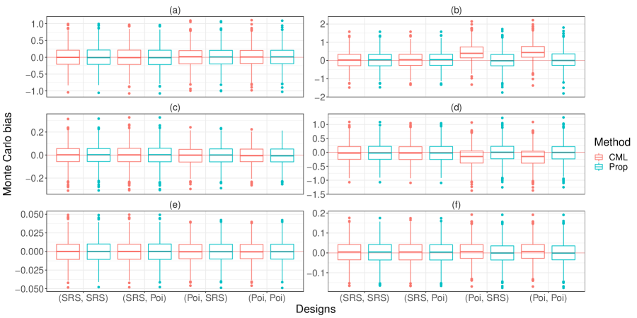
Figure 2: Monte Carlo bias of the proposed and CML estimators based on 1,000 Monte Carlo simulations under the homogeneous variance setup. The first to the third rows stand for the Monte Carlo bias for estimating $\beta_{0}$, $\beta_{1}$ and $\beta_{2}$, respectively. The three plots, including (a), (c) and (e), in the left column show the results when the auxiliary variables are independently generated, and those, including (b), (d) and (f), in the right column are for the case when the auxiliaries are dependent. “CML” and “Prop” stands for the CML estimator and the proposed estimator, respectively. The first design in the parenthesis is used to generate the internal sample $\mathcal{S}_{1}$, and the second one to generate the external sample $\mathcal{S}_{2}$. “Poi” represents Poisson sampling.

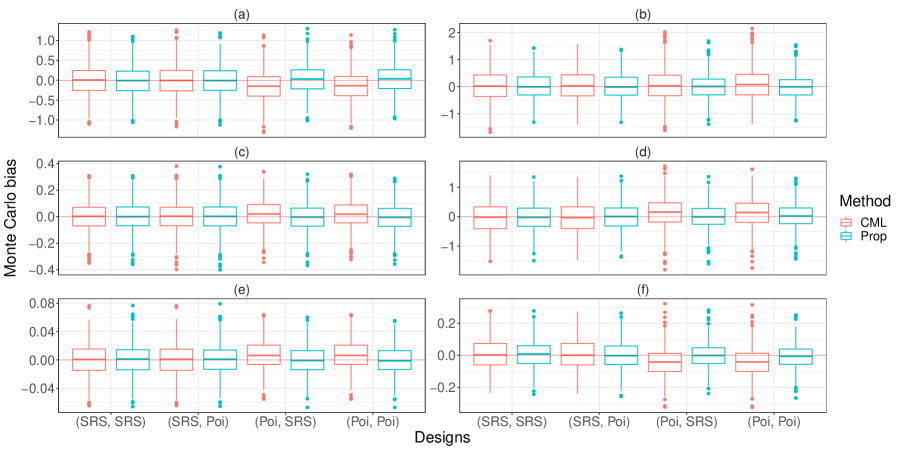
Figure 3: Monte Carlo bias of the proposed and CML estimators based on 1,000 Monte Carlo simulations under the heterogeneous variance setup. The first to the third rows stand for the Monte Carlo bias for estimating $\beta_{0}$, $\beta_{1}$ and $\beta_{2}$, respectively. The three plots, including (a), (c) and (e), in the left column show the results when the auxiliary variables are independently generated, and those, including (b), (d) and (f), in the right column are for the case when the auxiliaries are dependent. “CML” and “Prop” stands for the CML estimator and the proposed estimator, respectively. The first design in the parenthesis is used to generate the internal sample $\mathcal{S}_{1}$, and the second one to generate the external sample $\mathcal{S}_{2}$. “Poi” represents Poisson sampling.

Table 2 shows the coverage rate of a 95% confidence interval for the proposed estimator under different settings. Chatterjee et al. (2016) only investigated the theoretical properties of their estimator when the population-level information is available. Thus, no interval estimator can be provided if only an external sample is available. By Table 2, we conclude that the coverage rates of the confidence intervals are all close to its nominal truth 0.95 under different settings. One possible reason for this phenomenon is that the proposed estimator is model free, so the proposed model is more robust and can be used under complex sampling designs.

Table 2: Coverage rate of a 95% confidence interval by the proposed method based on 1,000 Monte Carlo simulations under different setups. “Homo” and “Hete” stands for the homogeneous and heterogeneous variance for the error term, respectively. “$\mathcal{S}_{1}$ Des” and “$\mathcal{S}_{2}$ Des” show the sampling design used to generate the internal sample $\mathcal{S}_{1}$ and the external sample $\mathcal{S}_{2}$. “SRS” and “Poi” stands for SRS and Poisson sampling, respectively. “Independent” and “Dependent” correspond to the cases when the auxiliary variables are independent and dependent, respectively.

	$\mathcal{S}_{1}$ Des	$\mathcal{S}_{2}$ Des	Independent				Dependent
			$\beta_{0}$	$\beta_{1}$	$\beta_{2}$		$\beta_{0}$	$\beta_{1}$	$\beta_{2}$
Homo	SRS	SRS	0.948	0.952	0.939		0.945	0.948	0.934
		Poi	0.945	0.951	0.938		0.946	0.946	0.934
	Poi	SRS	0.957	0.966	0.949		0.935	0.943	0.940
		Poi	0.962	0.964	0.951		0.936	0.943	0.938
Hete	SRS	SRS	0.944	0.942	0.933		0.933	0.925	0.935
		Poi	0.949	0.942	0.935		0.935	0.934	0.931
	Poi	SRS	0.959	0.955	0.935		0.948	0.950	0.941
		Poi	0.961	0.956	0.944		0.952	0.949	0.946

An additional simulation with a logistic regression setup is relegated to S3 of the Supplementary Material, and similar conclusions can be reached.

7 Application Study

7.1 Data Description and Problem Formulation

As an application example, we apply the proposed method to analyze a subset of the data from the Korea National Health and Nutrition Examination Survey (KNHANES). The annual survey includes approximately 5,000 individuals each year and collects information regarding health-related behaviors by interviews, basic health conditions by physical and blood tests, and dietary intake by nutrition survey. The sampling design of KNHANES is a stratified sampling using age, sex, and region as stratification variables. The final sampling weights are computed via nonresponse adjustment and post-stratification, then provided to data users with survey variables.

To improve the efficiency of data analysis with KNHANES of size $n_{1}=4{,}929$, we used an external public database provided by the National Health Insurance Sharing Service (NHISS) in Korea. The big data provided by NHISS contain about $n_{2}=1{,}000{,}000$ individuals with health-related information, some of whose variables are a subset of variables in KNHANES.

These data structures, with the small $n_{1}$, the large $n_{2}$, and the big data having a subset of variables in the internal sample, are suited well to the setting we addressed in Section 2. However, there is another complication in applying the proposed method to the real application. In the NHISS data, its selection probabilities are unknown, so the design consistent estimator $\hat{\mbox{\boldmath{$\alpha$}}}_{2}$ in (14) is unavailable. Section 7.2 addresses this issue by using a propensity weighting approach and Section 7.3 presents the analysis result of the application study.

7.2 Propensity Weighing for External Data with Unknown Selection Probability

We now consider an extension of the proposed method to the case where the external sample $\mathcal{S}_{2}$ is a big data with unknown selection probabilities. In this case, the working model for $E(Y_{i}\mid\mbox{\boldmath{$x$}}_{i1})=m(\mbox{\boldmath{$\alpha$}}^{\top}\mbox{\boldmath{$x$}}_{i1})$ may not hold for the sample $S_{2}$. Nonetheless, we may still solve

$$\sum_{i\in\mathcal{S}_{2}}\{y_{i}-m(\mbox{\boldmath{$\alpha$}}^{\top}\mbox{\boldmath{$x$}}_{i1})\}\mbox{\boldmath{$x$}}_{i1}=\mbox{\boldmath{$0$}}$$ (23)

to obtain $\hat{\alpha}_{0}$ and $\hat{\alpha}_{1}$. If the sampling mechanism for $\mathcal{S}_{2}$ is ignorable or non-informative, then the solution of (23) is unbiased; otherwise, the resulting estimator is biased.

To remove the selection biases in the big data estimate, Kim and Wang (2019) suggested using propensity score weights in (23) to obtain an unbiased estimator of $\alpha$. To construct the propensity score weights, we employ a nonignorable nonresponse model, $P(\delta_{i}=1\mid\mbox{\boldmath{$x$}}_{i1},y_{i})=\pi(\mbox{\boldmath{$x$}}_{i1},y_{i};\mbox{\boldmath{$\phi$}})$, where $\delta_{i}=1$ if $i\in S_{2}$ and zero otherwise. Note that we can express $\pi(\mbox{\boldmath{$x$}}_{i1},y_{i})^{-1}=1+(N_{0}/N_{1})r(\mbox{\boldmath{$x$}}_{i1},y_{i})$ where $r(\mbox{\boldmath{$x$}}_{i1},y_{i})=f(\mbox{\boldmath{$x$}}_{i1},y_{i}|\delta_{i}=0)/f(\mbox{\boldmath{$x$}}_{i1},y_{i}|\delta_{i}=1)$ is the density ratio function with $N_{1}=\sum_{i=1}^{N}\delta_{i}$ and $N_{0}=N-N_{1}$. Using the motivation of Wang and Kim (2021), we may assume a log-linear density ratio model, $\log\{r(x_{i1},y_{i};\mbox{\boldmath{$\phi$}})\}=\phi_{0}+\phi_{1}x_{i1}+\phi_{2}y_{i}$. The maximum entropy estimator of $\phi$ is obtained by solving $(1/N_{1})\sum_{i=1}^{N}\delta_{i}\exp(\phi_{0}+\phi_{1}x_{i1}+\phi_{2}y_{i})(1,x_{i1},y_{i})=\left(1,\hat{\bar{x}}_{1},\hat{\bar{y}}\right)$ where $(\hat{\bar{x}}_{1},\hat{\bar{y}})=(1/\hat{N}_{0})\left\{\sum_{i\in\mathcal{S}_{1}}d_{i}(x_{i1},y_{i})-\sum_{i=1}^{N}\delta_{i}(x_{i1},y_{i})\right\}$ and $\hat{N}_{0}=\sum_{i\in S_{1}}d_{i}-N_{1}$ where $\mathcal{S}_{1}$ is the internal sample. Once $\hat{\mbox{\boldmath{$\phi$}}}$ is obtained, we can construct $\hat{\pi}(x_{i1},y_{i})$ and solve

$$\sum_{i\in\mathcal{S}_{2}}\frac{1}{\hat{\pi}(x_{i1},y_{i})}\{y_{i}-m(\alpha_{0}+\alpha_{1}x_{i1})\}(1,x_{i1})=(0,0)$$ (24)

to obtain $\hat{\mbox{\boldmath{$\alpha$}}}_{2}=(\hat{\alpha}_{0},\hat{\alpha}_{1})$.

In addition, we can use the internal sample $\mathcal{S}_{1}$ to fit the same working model to obtain $\hat{\mbox{\boldmath{$\alpha$}}}_{1}$. After that, we obtain $\hat{\mbox{\boldmath{$\alpha$}}}^{*}$ using (14) and apply the proposed calibration weighting method to combine information from the big data. In practice, $\mbox{\boldmath{$V$}}_{2}$ in (14) is difficult to compute, but it is negligibly small if the sample size for $S_{2}$ is huge. In this case, we may simply use $\hat{\mbox{\boldmath{$\alpha$}}}^{*}=\hat{\mbox{\boldmath{$\alpha$}}}_{2}$ in the calibration problem.

7.3 Application Study Results: Korea National Health and Nutrition Examination Survey

In this application study, we use $n_{1}=4{,}929$ records of KNHANES data that have no missing values in four variables: Total cholesterol, Hemoglobin, Triglyceride, and high-density lipoprotein (HDL) cholesterol. For demonstration purpose, we assume that an analyst is interested in conducing the following linear regression analysis,

$$E(\text{Total Cholesterol}_{i}|\mbox{\boldmath{$x$}}_{i})=\beta_{0}+\beta_{1}\text{Hemoglobin}_{i}+\beta_{2}\text{Triglyceride}_{i}+\beta_{3}\text{HDL}_{i}\mbox{$\phantom{BB}$}\text{for }i\in\mathcal{S}_{1};$$

check Section S4 of the Supplementary Material for details about the linearity assumption. In our data, the biggest absolute value of the pairwise correlation among covariates is -0.40 observed between Triglyceride and HDL cholesterol, which is similar to a scenario in Section 6 where the covariates were highly correlated. The big external data consist of $n_{2}=1,000,000$ records of NHISS data with fully observed items in Total cholesterol, Hemoglobin, and Triglyceride. The assumed working reduced model is

$$E(\text{Total Cholesterol}_{i}|\mbox{\boldmath{$x$}}_{i1})=\alpha_{0}+\alpha_{1}\text{Hemoglobin}_{i}+\alpha_{2}\text{Triglyceride}_{i}\mbox{$\phantom{BB}$}\text{for }i\in\mathcal{S}_{1}\cup\mathcal{S}_{2}.$$

In this application study, we implement our proposed methods with the external sample where $\hat{\mbox{\boldmath{$\alpha$}}}_{2}$ is used instead of $\mbox{\boldmath{$\alpha$}}^{*}$ that is unavailable as we do not have information regarding the entire population. With the external sample whose selection probabilities are unknown, we prepare two versions of proposed methods: (i) considering $\mathcal{S}_{2}$ as SRS, i.e., without propensity weighting, and (ii) with the propensity weighting adjustment introduced in Section 7.2. For the propensity weighting, we fit the log-linear density ratio model to the external data, $\log\{r(\mbox{\boldmath{$x$}}_{i1},y_{i};\mbox{\boldmath{$\phi$}})\}=\phi_{0}+\phi_{1}\text{Hemoglobin}_{i}+\phi_{2}\text{Triglyceride}_{i}+\phi_{3}\text{Total Cholesterol}_{i}$, calculate $\hat{\pi}(\mbox{\boldmath{$x$}}_{i1},y_{i})$ given $\hat{\mbox{\boldmath{$\phi$}}}$, then solve (24) to obtain $\hat{\mbox{\boldmath{$\alpha$}}}_{2}$. The above logistic regression model is commonly assumed in the literure; see Elliott et al. (2017), Chen et al. (2020), Wang and Kim (2021) and the references within for details. Since the CML estimator fails to incorporate the design features, it is not considered in the application section. The performances of proposed methods are compared with the reference method that uses the internal sample $\mathcal{S}_{1}$ only to get weighted least square estimates considering the sampling weights.

Figure 4 shows the point estimates and the 95% confidence intervals of $\hat{\mbox{\boldmath{$\beta$}}}=(\hat{\beta}_{0},\hat{\beta}_{1},\hat{\beta}_{2},\hat{\beta}_{3})$ for each method. The proposed methods show smaller variances for $\hat{\beta}_{0}$, $\hat{\beta}_{1}$ and $\hat{\beta}_{2}$ than using the internal sample only. This result coincides with our findings in the simulation studies of the previous section. For $\beta_{2}$, the estimator of the proposed method without propensity weighting shows a systematic difference from the other two estimators. When the propensity weighting adjustment is coupled with the proposed method, its confidence interval of $\beta_{2}$ is contained by that of using the internal sample only. This result implies that the systematic bias due to the disregard of the sampling probabilities is addressed by the propensity weighting adjustment. No efficiency gain in estimating $\beta_{3}$ was expected as the external data contain information of $x_{i1}$ (Hemoglobin) and $x_{i2}$ (Triglyceride), not $x_{i3}$ (HDL).

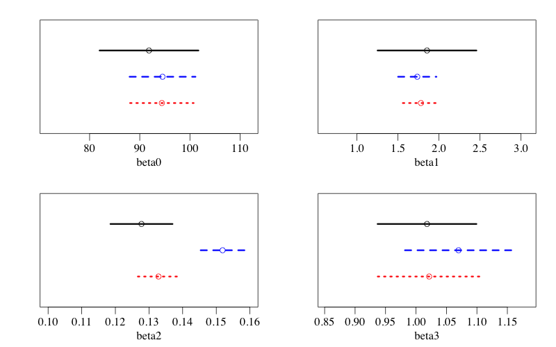
Figure 4: Comparison of the regression analysis for $E(\text{Total Cholesterol}_{i}|\mbox{\boldmath{$x$}}_{i})=\beta_{0}+\beta_{1}\text{Hemoglobin}_{i}+\beta_{2}\text{Triglyceride}_{i}+\beta_{3}\text{HDL}_{i}$ using the internal data from Korea National Health and Nutrition Examination Survey supported by the big external data from the National Health Insurance Sharing Service database. For each panel, circles are point estimates and lines are their 95% confidence intervals for using the internal sample $\mathcal{S}_{1}$ only with the weighted least square (top solid line), the proposed method without adjustment (middle dashed line), and the proposed method with propensity score weighting adjustment (bottom dotted line).

8 Conclusion

Incorporating external data sources into the regression analysis of the internal sample is an important practical problem. We have addressed this problem using a novel application of the information projection (Csiszár and Shields, 2004) and the model calibration weighting (Wu and Sitter, 2001). The proposed method is directly applicable to survey sampling and can be easily extended to multiple data integration. The proposed method is easy to implement and does not require direct access to external data. As long as the estimated regression coefficients and their standard errors for the working reduced model are available, we can incorporate the extra information into our analysis.

There are several possible directions on future research extensions. First, a Bayesian approach can be developed under the same setup. One may use the Bayesian empirical likelihood method of Zhao, Ghosh, Rao, and Wu (2020) in this setup. The proposed method can potentially be used to combine the randomized clinical trial data with big real-world data (Yang et al., 2020); such extensions will be presented elsewhere. It will be also interesting to connect the proposed approach to two-phase (double) sampling design whose efficient design and estimation has been recently studied actively (Rivera-Rodriguez, Spiegelman, and Haneuse, 2019, 2020; Wang, Williams, Chen, and Chen, 2020). The data structure of the two-phase sampling with the large-$n$, small-$p$ first stage sample and the small-$n$, large-$p$ second stage sample is well suited to the set-up assumed by the suggested model calibration approach.

Appendix

Appendix A Proof of Theorem 1

Lemma A1.

Suppose that conditions C1, C2e and C3 hold. Then, $\lVert\hat{\mbox{\boldmath{$\lambda$}}}\rVert=O_{p}(n^{-1/2})$.

Proof of Lemma A1.

Denote $\hat{\boldsymbol{\lambda}}=\rho\boldsymbol{\theta}$, where $\rho=\lVert\hat{\boldsymbol{\lambda}}\rVert$ and $\boldsymbol{\theta}=\rho^{-1}\hat{\boldsymbol{\lambda}}$ is a vector of unit length. Then, we have

$\mathrm{𝟎}$ $\displaystyle=$ $\displaystyle\left\lvert\sum_{i\in\mathcal{S}_{1}}\frac{\tilde{d}_{i}}{1-\hat{\boldsymbol{\lambda}}^{{\mathrm{\scriptscriptstyle T}}}\mbox{\boldmath{$U$}}_{2}({\mbox{\boldmath$\alpha$}}_{N}^{*};\mbox{\boldmath{$x$}}_{1i},y_{i})}\mbox{\boldmath{$U$}}_{2}({\mbox{\boldmath$\alpha$}}_{N}^{*};\mbox{\boldmath{$x$}}_{1i},y_{i})\right\rvert$

$$= \left\lvert\boldsymbol{\theta}^{{\mathrm{\scriptscriptstyle T}}}\sum_{i\in\mathcal{S}_{1}}\frac{\tilde{d}_{i}}{1-\rho\boldsymbol{\theta}^{{\mathrm{\scriptscriptstyle T}}}\mbox{\boldmath{$U$}}_{2}({\mbox{\boldmath$\alpha$}}_{N}^{*};\mbox{\boldmath{$x$}}_{1i},y_{i})}\mbox{\boldmath{$U$}}_{2}({\mbox{\boldmath$\alpha$}}_{N}^{*};\mbox{\boldmath{$x$}}_{1i},y_{i})\right\rvert$$

$$= \left\lvert\sum_{i\in\mathcal{S}_{1}}\tilde{d}_{i}\boldsymbol{\theta}^{{\mathrm{\scriptscriptstyle T}}}\mbox{\boldmath{$U$}}_{2}({\mbox{\boldmath$\alpha$}}_{N}^{*};\mbox{\boldmath{$x$}}_{1i},y_{i})+\rho\sum_{i\in\mathcal{S}_{1}}\frac{\tilde{d}_{i}\boldsymbol{\theta}^{{\mathrm{\scriptscriptstyle T}}}\mbox{\boldmath{$U$}}_{2}({\mbox{\boldmath$\alpha$}}_{N}^{*};\mbox{\boldmath{$x$}}_{1i},y_{i})\{\mbox{\boldmath{$U$}}_{2}({\mbox{\boldmath$\alpha$}}_{N}^{*};\mbox{\boldmath{$x$}}_{1i},y_{i})\}^{{\mathrm{\scriptscriptstyle T}}}\boldsymbol{\theta}}{1-\rho\boldsymbol{\theta}^{{\mathrm{\scriptscriptstyle T}}}\mbox{\boldmath{$U$}}_{2}({\mbox{\boldmath$\alpha$}}_{N}^{*};\mbox{\boldmath{$x$}}_{1i},y_{i})}\right\rvert$$

$$\geq \frac{\rho}{1+\rho Z_{S}}\left\lvert\sum_{i\in\mathcal{S}_{1}}\tilde{d_{i}}\boldsymbol{\theta}^{{\mathrm{\scriptscriptstyle T}}}\mbox{\boldmath{$U$}}_{2}({\mbox{\boldmath$\alpha$}}_{N}^{*};\mbox{\boldmath{$x$}}_{1i},y_{i})\{\mbox{\boldmath{$U$}}_{2}({\mbox{\boldmath$\alpha$}}_{N}^{*};\mbox{\boldmath{$x$}}_{1i},y_{i})\}^{{\mathrm{\scriptscriptstyle T}}}\boldsymbol{\theta}\right\rvert-\left\lvert\sum_{i\in\mathcal{S}_{1}}\tilde{d}_{i}\boldsymbol{\theta}^{{\mathrm{\scriptscriptstyle T}}}\mbox{\boldmath{$U$}}_{2}({\mbox{\boldmath$\alpha$}}_{N}^{*};\mbox{\boldmath{$x$}}_{1i},y_{i})\right\rvert,$$

where the first equality holds since $g(\hat{\boldsymbol{\eta}})=\mbox{\boldmath{$0$}}$, the last inequality holds by the triangular inequality.

By C2e and the Rayleigh-Ritz Theorem (Horn and Johnson, 2012, Section 4.2), there exists a constant $\sigma_{0}>0$ such that

$$\sum_{i\in\mathcal{S}_{1}}\tilde{d}_{i}\boldsymbol{\theta}^{{\mathrm{\scriptscriptstyle T}}}\mbox{\boldmath{$U$}}_{2}({\mbox{\boldmath$\alpha$}}_{N}^{*};\mbox{\boldmath{$x$}}_{1i},y_{i})\{\mbox{\boldmath{$U$}}_{2}({\mbox{\boldmath$\alpha$}}_{N}^{*};\mbox{\boldmath{$x$}}_{1i},y_{i})\}^{{\mathrm{\scriptscriptstyle T}}}\boldsymbol{\theta}>\sigma_{0}+o_{p}(1).$$ (A.2)

By C3 and the Slutsky’s theorem, we have

$$\sum_{i\in\mathcal{S}_{1}}\tilde{d}_{i}\boldsymbol{\theta}^{{\mathrm{\scriptscriptstyle T}}}\mbox{\boldmath{$U$}}_{2}({\mbox{\boldmath$\alpha$}}_{N}^{*};\mbox{\boldmath{$x$}}_{1i},y_{i})=O_{p}(n^{-1/2}).$$ (A.3)

Thus, by C1 and (LABEL:eq:_theorem_1_1)–(A.3), we have proved Lemma A1. ∎

Lemma A2.

Suppose that conditions C1, C2a–C2e and C3 hold. Then, $\hat{\mbox{\boldmath{$\beta$}}}-\mbox{\boldmath{$\beta$}}_{0N}=o_{p}(1)$.

Proof of Lemma A2.

By Lemma  A1 and C1, we conclude that

$$\max_{i\in\mathcal{S}_{1}}\lvert\hat{\boldsymbol{\lambda}}^{{\mathrm{\scriptscriptstyle T}}}\mbox{\boldmath{$U$}}_{2}({\mbox{\boldmath$\alpha$}}_{N}^{*};\mbox{\boldmath{$x$}}_{1i},y_{i})\rvert\leq\max_{i\in\mathcal{S}_{1}}\lVert\hat{\boldsymbol{\lambda}}\rVert\lVert\mbox{\boldmath{$U$}}_{2}({\mbox{\boldmath$\alpha$}}_{N}^{*};\mbox{\boldmath{$x$}}_{1i},y_{i})\rVert=\lVert\hat{\boldsymbol{\lambda}}\rVert\max_{i\in\mathcal{S}_{1}}\lVert\mbox{\boldmath{$U$}}_{2}({\mbox{\boldmath$\alpha$}}_{N}^{*};\mbox{\boldmath{$x$}}_{1i},y_{i})\rVert=o_{p}(1).$$ (A.4)

First, we show that

$$\sum_{i\in\mathcal{S}_{1}}\frac{\tilde{d}_{i}}{1-\hat{\boldsymbol{\lambda}}^{{\mathrm{\scriptscriptstyle T}}}\mbox{\boldmath{$U$}}_{2}({\mbox{\boldmath$\alpha$}}_{N}^{*};\mbox{\boldmath{$x$}}_{1i},y_{i})}\mbox{\boldmath{$U$}}_{1}(\mbox{\boldmath{$\beta$}};\mbox{\boldmath{$x$}}_{i},y_{i})-\sum_{i\in\mathcal{S}_{1}}\tilde{d}_{i}\mbox{\boldmath{$U$}}_{1}(\mbox{\boldmath{$\beta$}};\mbox{\boldmath{$x$}}_{i},y_{i})\to\mbox{\boldmath{$0$}}$$ (A.5)

in probability uniformly for ${\mbox{\boldmath$\beta$}}\in\Omega$. By (A.4), we have

$$\left\lVert\sum_{i\in\mathcal{S}_{1}}\tilde{d}_{i}\left\{\frac{1}{1-\hat{\boldsymbol{\lambda}}^{{\mathrm{\scriptscriptstyle T}}}\mbox{\boldmath{$U$}}_{2}({\mbox{\boldmath$\alpha$}}_{N}^{*};\mbox{\boldmath{$x$}}_{1i},y_{i})}-1\right\}\mbox{\boldmath{$U$}}_{1}(\mbox{\boldmath{$\beta$}};\mbox{\boldmath{$x$}}_{i},y_{i})\right\rVert$$ (A.6)

$$= \left\lVert\sum_{i\in\mathcal{S}_{1}}\tilde{d}_{i}\{\hat{\boldsymbol{\lambda}}^{{\mathrm{\scriptscriptstyle T}}}\mbox{\boldmath{$U$}}_{2}({\mbox{\boldmath$\alpha$}}_{N}^{*};\mbox{\boldmath{$x$}}_{1i},y_{i})+o_{p}(\hat{\boldsymbol{\lambda}}^{{\mathrm{\scriptscriptstyle T}}}\mbox{\boldmath{$U$}}_{2}({\mbox{\boldmath$\alpha$}}_{N}^{*};\mbox{\boldmath{$x$}}_{1i},y_{i}))\}\mbox{\boldmath{$U$}}_{1}(\mbox{\boldmath{$\beta$}};\mbox{\boldmath{$x$}}_{i},y_{i})\right\rVert$$

$$\leq (1+o_{p}(1))\max_{i\in\mathcal{S}_{1}}\lvert\hat{\boldsymbol{\lambda}}^{{\mathrm{\scriptscriptstyle T}}}\mbox{\boldmath{$U$}}_{2}({\mbox{\boldmath$\alpha$}}_{N}^{*};\mbox{\boldmath{$x$}}_{1i},y_{i})\rvert\left\lVert\sum_{i\in\mathcal{S}_{1}}\tilde{d}_{i}\mbox{\boldmath{$U$}}_{1}(\mbox{\boldmath{$\beta$}};\mbox{\boldmath{$x$}}_{i},y_{i})\right\rVert.$$

By C2a–C2b, there exists a constant $C_{u1}>0$ such that $\sup_{\boldsymbol{\beta}\in\Omega}\lVert\mbox{\boldmath{$U$}}_{0}({\mbox{\boldmath$\beta$}})\rVert<C_{u1}$. Since $\sum_{i\in\mathcal{S}_{1}}\tilde{d}_{i}\mbox{\boldmath{$U$}}_{1}(\mbox{\boldmath{$\beta$}};\mbox{\boldmath{$x$}}_{i},y_{i})$ converge uniformly to $\mbox{\boldmath{$U$}}_{0}({\mbox{\boldmath$\beta$}})$ in probability, we conclude that

$$\left\lVert\sum_{i\in\mathcal{S}_{1}}\tilde{d}_{i}\mbox{\boldmath{$U$}}_{1}(\mbox{\boldmath{$\beta$}};\mbox{\boldmath{$x$}}_{i},y_{i})\right\rVert<C_{u1}+o_{p}(1)$$ (A.7)

uniformly over $\Omega$. By (A.4) and (A.6)–(A.7), we have validated (A.5).

By C2b and (A.5), we conclude that $\sum_{i\in\mathcal{S}_{1}}\tilde{d}_{i}\{1-\hat{\boldsymbol{\lambda}}^{{\mathrm{\scriptscriptstyle T}}}\mbox{\boldmath{$U$}}_{2}({\mbox{\boldmath$\alpha$}}_{N}^{*};\mbox{\boldmath{$x$}}_{1i},y_{i})\}^{-1}\mbox{\boldmath{$U$}}_{1}(\mbox{\boldmath{$\beta$}};\mbox{\boldmath{$x$}}_{i},y_{i})$ converges uniformly to $U_{0}({\mbox{\boldmath$\beta$}})$ in probability. Denote $Q_{0}({\mbox{\boldmath$\beta$}})=-U_{0}({\mbox{\boldmath$\beta$}})^{2}$ and $Q_{s}({\mbox{\boldmath$\beta$}})=-[\sum_{i\in\mathcal{S}_{1}}\tilde{d}_{i}\{1-\hat{\boldsymbol{\lambda}}^{{\mathrm{\scriptscriptstyle T}}}\mbox{\boldmath{$U$}}_{2}({\mbox{\boldmath$\alpha$}}_{N}^{*};\mbox{\boldmath{$x$}}_{1i},y_{i})\}^{-1}\mbox{\boldmath{$U$}}_{1}(\mbox{\boldmath{$\beta$}};\mbox{\boldmath{$x$}}_{i},y_{i})]^{2}$. Then, ${\mbox{\boldmath$\beta$}}_{p}$ uniquely maximizes $Q_{0}({\mbox{\boldmath$\beta$}})$ by (C2b), and $\hat{{\mbox{\boldmath$\beta$}}}$ maximizes $Q_{s}({\mbox{\boldmath$\beta$}})$. In addition, $Q_{s}({\mbox{\boldmath$\beta$}})$ converge uniformly to $Q_{0}({\mbox{\boldmath$\beta$}})$ in probability over the compact set $\Omega$. Thus, by C2a and Theorem 2.1 of Engle and McFadden (1994, Chapter 36), we have finished the proof for Lemma A2. ∎

Proof of Theorem 1.

By Lemmas A1–A2, we have shown that

$$\hat{\boldsymbol{\eta}}=\boldsymbol{\eta}_{0}+o_{p}(1),$$ (A.8)

where $\hat{\boldsymbol{\eta}}^{{\mathrm{\scriptscriptstyle T}}}=(\hat{{\mbox{\boldmath$\beta$}}}^{{\mathrm{\scriptscriptstyle T}}},\hat{\boldsymbol{\lambda}}^{{\mathrm{\scriptscriptstyle T}}})$, $\boldsymbol{\eta}_{0}^{{\mathrm{\scriptscriptstyle T}}}=({\mbox{\boldmath$\beta$}}_{0N}^{{\mathrm{\scriptscriptstyle T}}},\boldsymbol{0}^{{\mathrm{\scriptscriptstyle T}}})$, and $\boldsymbol{0}$ is a vector of zero with the same length of $\hat{\boldsymbol{\lambda}}$.

By (A.8) and the Taylor expansion, we have

$\mathrm{𝟎}$ $\displaystyle=$ $\displaystyle g(\hat{\boldsymbol{\eta}})=g(\boldsymbol{\eta}_{0})+\frac{\partial g}{\partial\boldsymbol{\eta}^{{\mathrm{\scriptscriptstyle T}}}}(\boldsymbol{\eta}_{0})(\hat{\boldsymbol{\eta}}-\boldsymbol{\eta}_{0})+o_{p}(\lVert\hat{\boldsymbol{\eta}}-\boldsymbol{\eta}_{0}\rVert)$

$$= \begin{pmatrix}\displaystyle\sum_{i\in\mathcal{S}_{1}}\tilde{d}_{i}\mbox{\boldmath{$U$}}_{1}(\mbox{\boldmath{$\beta$}}_{0N};\mbox{\boldmath{$x$}}_{i},y_{i})\\ \displaystyle\sum_{i\in\mathcal{S}_{1}}\tilde{d}_{i}\mbox{\boldmath{$U$}}_{2}({\mbox{\boldmath$\alpha$}}_{N}^{*};\mbox{\boldmath{$x$}}_{1i},y_{i})\par\end{pmatrix}$$

$$+\begin{pmatrix}\displaystyle\sum_{i\in\mathcal{S}_{1}}\tilde{d}_{i}\frac{\partial\mbox{\boldmath{$U$}}_{1}(\mbox{\boldmath{$\beta$}}_{0N};\mbox{\boldmath{$x$}}_{i},y_{i})}{\partial{\mbox{\boldmath$\beta$}}^{{\mathrm{\scriptscriptstyle T}}}}&\displaystyle\sum_{i\in\mathcal{S}_{1}}\tilde{d}_{i}\mbox{\boldmath{$U$}}_{1}(\mbox{\boldmath{$\beta$}}_{0N};\mbox{\boldmath{$x$}}_{i},y_{i})\{\mbox{\boldmath{$U$}}_{2}({\mbox{\boldmath$\alpha$}}_{N}^{*};\mbox{\boldmath{$x$}}_{1i},y_{i})\}^{{\mathrm{\scriptscriptstyle T}}}\\ \mbox{\boldmath{$0$}}&\displaystyle\sum_{i\in\mathcal{S}_{1}}\tilde{d}_{i}\{\mbox{\boldmath{$U$}}_{2}({\mbox{\boldmath$\alpha$}}_{N}^{*};\mbox{\boldmath{$x$}}_{1i},y_{i})\}^{\otimes 2}\par\end{pmatrix}(\hat{\boldsymbol{\eta}}-\boldsymbol{\eta}_{0})$$

$$+o_{p}(\lVert\hat{\boldsymbol{\eta}}-\boldsymbol{\eta}_{0}\rVert).$$

By (C3), we have

$$n^{1/2}\begin{pmatrix}\displaystyle\sum_{i\in\mathcal{S}_{1}}\tilde{d}_{i}\mbox{\boldmath{$U$}}_{1}(\mbox{\boldmath{$\beta$}}_{0N};\mbox{\boldmath{$x$}}_{i},y_{i})\\ \displaystyle\sum_{i\in\mathcal{S}_{1}}\tilde{d}_{i}\mbox{\boldmath{$U$}}_{2}({\mbox{\boldmath$\alpha$}}_{N}^{*};\mbox{\boldmath{$x$}}_{1i},y_{i})\par\end{pmatrix}\to\mathcal{N}(\mbox{\boldmath{$0$}},\mbox{\boldmath{$\Sigma$}}_{u})$$ (A.10)

in distribution. By (C2e)–(C2c), we conclude that

$$\begin{pmatrix}\displaystyle\sum_{i\in\mathcal{S}_{1}}\tilde{d}_{i}\frac{\partial\mbox{\boldmath{$U$}}_{1}(\mbox{\boldmath{$\beta$}}_{0N};\mbox{\boldmath{$x$}}_{i},y_{i})}{\partial{\mbox{\boldmath$\beta$}}^{{\mathrm{\scriptscriptstyle T}}}}&\displaystyle\sum_{i\in\mathcal{S}_{1}}\tilde{d}_{i}\mbox{\boldmath{$U$}}_{1}(\mbox{\boldmath{$\beta$}}_{0N};\mbox{\boldmath{$x$}}_{i},y_{i})\{\mbox{\boldmath{$U$}}_{2}({\mbox{\boldmath$\alpha$}}_{N}^{*};\mbox{\boldmath{$x$}}_{1i},y_{i})\}^{{\mathrm{\scriptscriptstyle T}}}\\ \mbox{\boldmath{$0$}}&\displaystyle\sum_{i\in\mathcal{S}_{1}}\tilde{d}_{i}\{\mbox{\boldmath{$U$}}_{2}({\mbox{\boldmath$\alpha$}}_{N}^{*};\mbox{\boldmath{$x$}}_{1i},y_{i})\}^{\otimes 2}\end{pmatrix}\to\boldsymbol{\mathcal{I}}$$ (A.11)

in probability, where

$$\boldsymbol{\mathcal{I}}=\begin{pmatrix}\boldsymbol{\mathcal{I}}_{11}&\boldsymbol{\mathcal{I}}_{12}\\ \mbox{\boldmath{$0$}}&\boldsymbol{\mathcal{I}}_{22}\end{pmatrix}.$$

By (LABEL:eq:_theorem_3_CLT_1)–(A.11), we conclude that

$$n^{1/2}(\hat{\boldsymbol{\eta}}-\boldsymbol{\eta}_{0})\to\mathcal{N}(\mbox{\boldmath{$0$}},\mbox{\boldmath{$\Sigma$}}_{\eta})$$ (A.12)

in distribution, where $\mbox{\boldmath{$\Sigma$}}_{\eta}=\boldsymbol{\mathcal{I}}^{-1}\mbox{\boldmath{$\Sigma$}}_{u}(\boldsymbol{\mathcal{I}}^{-1})^{{\mathrm{\scriptscriptstyle T}}}.$ ∎

Appendix B Proof of Corollary 1

Since $\mbox{\boldmath{$U$}}_{1}(\mbox{\boldmath{$\beta$}};\mbox{\boldmath{$x$}},y)$ is given, it is enough to consider

$$\mbox{\boldmath{$\Sigma$}}_{11}-\boldsymbol{\mathcal{I}}_{12}\boldsymbol{\mathcal{I}}_{22}^{-1}\mbox{\boldmath{$\Sigma$}}_{21}-\mbox{\boldmath{$\Sigma$}}_{12}\boldsymbol{\mathcal{I}}_{22}^{-1}\boldsymbol{\mathcal{I}}_{12}^{{\mathrm{\scriptscriptstyle T}}}+\boldsymbol{\mathcal{I}}_{12}\boldsymbol{\mathcal{I}}_{22}^{-1}\mbox{\boldmath{$\Sigma$}}_{22}\boldsymbol{\mathcal{I}}_{22}^{-1}\boldsymbol{\mathcal{I}}_{12}^{{\mathrm{\scriptscriptstyle T}}},$$

the asymptotic variance of $\tilde{\mbox{\boldmath{$U$}}}_{1}(\mbox{\boldmath{$\beta$}}_{0N})-\boldsymbol{\mathcal{I}}_{12}\boldsymbol{\mathcal{I}}_{22}^{-1}\tilde{\mbox{\boldmath{$U$}}}_{2}(\mbox{\boldmath{$\alpha$}}_{N}^{*})$, where $\tilde{\mbox{\boldmath{$U$}}}_{1}(\mbox{\boldmath{$\beta$}}_{0N})=n^{1/2}\sum_{i\in\mathcal{S}_{1}}\tilde{d}_{i}\mbox{\boldmath{$U$}}_{1}(\mbox{\boldmath{$\beta$}}_{0N};\mbox{\boldmath{$x$}}_{i},y_{i})$ and $\tilde{\mbox{\boldmath{$U$}}}_{2}(\mbox{\boldmath{$\alpha$}}_{N}^{*})=n^{1/2}\sum_{i\in\mathcal{S}_{1}}\tilde{d}_{i}\mbox{\boldmath{$U$}}_{2}(\mbox{\boldmath{$\alpha$}}_{N}^{*};\mbox{\boldmath{$x$}}_{i1},y_{i})$.

Consider

$$\mathrm{Var}\{\tilde{\mbox{\boldmath{$U$}}}_{1}(\mbox{\boldmath{$\beta$}}_{0N})-\boldsymbol{\mathcal{I}}_{12}\boldsymbol{\mathcal{I}}_{22}^{-1}\tilde{\mbox{\boldmath{$U$}}}_{2}(\mbox{\boldmath{$\alpha$}}_{N}^{*})\}$$

$$= E[\mathrm{Var}\{\tilde{\mbox{\boldmath{$U$}}}_{1}(\mbox{\boldmath{$\beta$}}_{0N})-\boldsymbol{\mathcal{I}}_{12}\boldsymbol{\mathcal{I}}_{22}^{-1}\tilde{\mbox{\boldmath{$U$}}}_{2}(\mbox{\boldmath{$\alpha$}}_{N}^{*})\mid\mathcal{A}_{N}\}]+\mathrm{Var}[E\{\tilde{\mbox{\boldmath{$U$}}}_{1}(\mbox{\boldmath{$\beta$}}_{0N})-\boldsymbol{\mathcal{I}}_{12}\boldsymbol{\mathcal{I}}_{22}^{-1}\tilde{\mbox{\boldmath{$U$}}}_{2}(\mbox{\boldmath{$\alpha$}}_{N}^{*})\mid\mathcal{A}_{N}\}]$$

$$\succcurlyeq E[\mathrm{Var}\{\tilde{\mbox{\boldmath{$U$}}}_{1}(\mbox{\boldmath{$\beta$}}_{0N})\}],$$

where $\mathcal{A}_{N}=\{(\mbox{\boldmath{$x$}}_{i1},y):i\in\mathcal{S}_{1}\}$, $A\succcurlyeq B$ is equivalent to that $A-B$ is non-negatively definitive for two matrices $A$ and $B$ with the same dimension, the last inequality holds since $\tilde{\mbox{\boldmath{$U$}}}_{2}(\mbox{\boldmath{$\alpha$}}_{N}^{*})$ is non-stochastic conditional on $\mathcal{A}_{N}$. Thus, $\mathrm{Var}\{\tilde{\mbox{\boldmath{$U$}}}_{1}(\mbox{\boldmath{$\beta$}}_{0N})-\boldsymbol{\mathcal{I}}_{12}\boldsymbol{\mathcal{I}}_{22}^{-1}\tilde{\mbox{\boldmath{$U$}}}_{2}(\mbox{\boldmath{$\alpha$}}_{N}^{*})\}$ achieves minimum if $\mathrm{Var}[E\{\tilde{\mbox{\boldmath{$U$}}}_{1}(\mbox{\boldmath{$\beta$}}_{0N})-\boldsymbol{\mathcal{I}}_{12}\boldsymbol{\mathcal{I}}_{22}^{-1}\tilde{\mbox{\boldmath{$U$}}}_{2}(\mbox{\boldmath{$\alpha$}}_{N}^{*})\mid\mathcal{A}_{N}\}]=0$, which is induced by the condition $\boldsymbol{\mathcal{I}}_{12}\boldsymbol{\mathcal{I}}_{22}^{-1}\mbox{\boldmath{$U$}}_{2}(\mbox{\boldmath{$\alpha$}}_{N}^{*};\mbox{\boldmath{$x$}}_{1},y)=E\{\mbox{\boldmath{$U$}}_{1}(\mbox{\boldmath{$\beta$}}_{0N};\mbox{\boldmath{$x$}},y)\mid\mbox{\boldmath{$x$}}_{1},y\}$.

Appendix C Proof of Theorem 2

Before proving Theorem 2, we need the following result.

Lemma A3.

Suppose that conditions C1, C3–C5 hold. Then, we have

$$\hat{{\mbox{\boldmath$\alpha$}}}^{*}-{\mbox{\boldmath$\alpha$}}^{*}_{N}=O_{p}(n^{-1/2}),$$

Proof of Lemma A3.

Since $\hat{{\mbox{\boldmath$\alpha$}}}_{2}$ is obtained by an independent external survey, we conclude that the variance of $\hat{{\mbox{\boldmath$\alpha$}}}^{*}$ can be estimated by $(\mbox{\boldmath{$V$}}_{1}^{-1}+\mbox{\boldmath{$V$}}_{2}^{-1})^{-1}$. Thus, the order of the variance of $\hat{{\mbox{\boldmath$\alpha$}}}^{*}$ is determined by the less efficient estimator between $\hat{{\mbox{\boldmath$\alpha$}}}_{1}$ and $\hat{{\mbox{\boldmath$\alpha$}}}_{2}$. If we showed

$$\hat{{\mbox{\boldmath$\alpha$}}}_{1}-{\mbox{\boldmath$\alpha$}}^{*}_{N}=O_{p}(n^{-1/2}),$$ (A.13)

we could have $\mbox{\boldmath{$V$}}_{1}=O_{p}(n^{-1})$ by (C5b). Since $\hat{{\mbox{\boldmath$\alpha$}}}^{*}$ is at least as efficient as $\hat{{\mbox{\boldmath$\alpha$}}}_{1}$, we have completed the proof of Lemma A3.

Thus, it remains to show (A.13). By C4 and C5, we have

$\mathrm{𝟎}$ $\displaystyle=$ $\displaystyle\sum_{i\in\mathcal{S}_{1}}\tilde{d}_{i}\mbox{\boldmath{$U$}}_{2}(\hat{{\mbox{\boldmath$\alpha$}}}_{1};\mbox{\boldmath{$x$}}_{1i},y_{i})$

$$= \sum_{i\in\mathcal{S}_{1}}\tilde{d}_{i}\mbox{\boldmath{$U$}}_{2}({\mbox{\boldmath$\alpha$}}_{N}^{*};\mbox{\boldmath{$x$}}_{1i},y_{i})+\left\{\frac{\partial}{\partial{\mbox{\boldmath$\alpha$}}^{{\mathrm{\scriptscriptstyle T}}}}\sum_{i\in\mathcal{S}_{1}}\tilde{d}_{i}\mbox{\boldmath{$U$}}_{2}(\tilde{\mbox{\boldmath{$\alpha$}}};\mbox{\boldmath{$x$}}_{1i},y_{i})\right\}(\hat{\mbox{\boldmath{$\alpha$}}}_{1}-{\mbox{\boldmath$\alpha$}}^{*}_{N}),$$

where $\tilde{{\mbox{\boldmath$\alpha$}}}$ lies on the segment joining $\hat{\mbox{\boldmath{$\alpha$}}}_{1}$ and ${\mbox{\boldmath$\alpha$}}^{*}_{N}$. By C3–C5 and (LABEL:eq:_U1_alpha_1_=0), we conclude that

$$\hat{{\mbox{\boldmath$\alpha$}}}-{\mbox{\boldmath$\alpha$}}^{*}_{N}=-\boldsymbol{\mathcal{I}}_{0}^{-1}\sum_{i\in\mathcal{S}_{1}}\tilde{d}_{i}\mbox{\boldmath{$U$}}_{2}({\mbox{\boldmath$\alpha$}}_{N}^{*};\mbox{\boldmath{$x$}}_{1i},y_{i})+o_{p}(n^{-1/2}).$$ (A.15)

Thus, by C3 and (A.15), we have shown (A.13). ∎

Proof of Theorem 2.

Consider

$$\sum_{i\in\mathcal{S}_{1}}\tilde{d}_{i}\mbox{\boldmath{$U$}}_{2}(\hat{{\mbox{\boldmath$\alpha$}}}^{*};\mbox{\boldmath{$x$}}_{1i},y_{i})$$ (A.16)

$$= \sum_{i\in\mathcal{S}_{1}}\tilde{d}_{i}\mbox{\boldmath{$U$}}_{2}({\mbox{\boldmath$\alpha$}}_{N}^{*};\mbox{\boldmath{$x$}}_{1i},y_{i})+\left\{\frac{\partial}{\partial{\mbox{\boldmath$\alpha$}}^{{\mathrm{\scriptscriptstyle T}}}}\sum_{i\in\mathcal{S}_{1}}\tilde{d}_{i}\mbox{\boldmath{$U$}}_{2}(\tilde{{\mbox{\boldmath$\alpha$}}};x_{1i},y_{i})\right\}(\hat{{\mbox{\boldmath$\alpha$}}}^{*}-{\mbox{\boldmath$\alpha$}}_{N}^{*})$$

$$= \sum_{i\in\mathcal{S}_{1}}\tilde{d}_{i}\mbox{\boldmath{$U$}}_{2}({\mbox{\boldmath$\alpha$}}_{N}^{*};\mbox{\boldmath{$x$}}_{1i},y_{i})+\boldsymbol{\mathcal{I}}_{0}(\mbox{\boldmath{$V$}}_{1}^{-1}+\mbox{\boldmath{$V$}}_{2}^{-1})^{-1}\mbox{\boldmath{$V$}}_{2}^{-1}(\hat{{\mbox{\boldmath$\alpha$}}}_{2}-{\mbox{\boldmath$\alpha$}}^{*}_{N})$$

$$+\boldsymbol{\mathcal{I}}_{0}(\mbox{\boldmath{$V$}}_{1}^{-1}+\mbox{\boldmath{$V$}}_{2}^{-1})^{-1}\mbox{\boldmath{$V$}}_{1}^{-1}(\hat{{\mbox{\boldmath$\alpha$}}}-{\mbox{\boldmath$\alpha$}}^{*}_{N})+o_{p}(n^{-1/2}),$$

$$= \sum_{i\in\mathcal{S}_{1}}\tilde{d}_{i}\mbox{\boldmath{$U$}}_{2}({\mbox{\boldmath$\alpha$}}_{N}^{*};\mbox{\boldmath{$x$}}_{1i},y_{i})+\boldsymbol{\mathcal{I}}_{0}(\mbox{\boldmath{$V$}}_{1}^{-1}+\mbox{\boldmath{$V$}}_{2}^{-1})^{-1}\mbox{\boldmath{$V$}}_{2}^{-1}(\hat{{\mbox{\boldmath$\alpha$}}}_{2}-{\mbox{\boldmath$\alpha$}}^{*}_{N})$$

$$-\boldsymbol{\mathcal{I}}_{0}(\mbox{\boldmath{$V$}}_{1}^{-1}+\mbox{\boldmath{$V$}}_{2}^{-1})^{-1}\mbox{\boldmath{$V$}}_{1}^{-1}\boldsymbol{\mathcal{I}}_{0}^{-1}\sum_{i\in\mathcal{S}_{1}}\tilde{d}_{i}\mbox{\boldmath{$U$}}_{2}({\mbox{\boldmath$\alpha$}}_{N}^{*};\mbox{\boldmath{$x$}}_{1i},y_{i})+o_{p}(n^{-1/2}),$$

$$= \boldsymbol{\mathcal{I}}_{0}(\mbox{\boldmath{$V$}}_{1}^{-1}+\mbox{\boldmath{$V$}}_{2}^{-1})^{-1}\mbox{\boldmath{$V$}}_{2}^{-1}(\hat{{\mbox{\boldmath$\alpha$}}}_{2}-{\mbox{\boldmath$\alpha$}}^{*}_{N})+\boldsymbol{\mathcal{I}}_{0}(\mbox{\boldmath{$V$}}_{1}^{-1}+\mbox{\boldmath{$V$}}_{2}^{-1})^{-1}\mbox{\boldmath{$V$}}_{2}^{-1}\boldsymbol{\mathcal{I}}_{0}^{-1}\sum_{i\in\mathcal{S}_{1}}\tilde{d}_{i}\mbox{\boldmath{$U$}}_{2}({\mbox{\boldmath$\alpha$}}_{N}^{*};\mbox{\boldmath{$x$}}_{1i},y_{i})$$

$$+o_{p}(n^{-1/2})$$

$$= \boldsymbol{\mathcal{I}}_{0}\mbox{\boldmath{$W$}}(\hat{{\mbox{\boldmath$\alpha$}}}_{2}-{\mbox{\boldmath$\alpha$}}^{*}_{N})+\boldsymbol{\mathcal{I}}_{0}\mbox{\boldmath{$W$}}\boldsymbol{\mathcal{I}}_{0}^{-1}\sum_{i\in\mathcal{S}_{1}}\tilde{d}_{i}\mbox{\boldmath{$U$}}_{2}({\mbox{\boldmath$\alpha$}}_{N}^{*};\mbox{\boldmath{$x$}}_{1i},y_{i})+o_{p}(\kappa(n)),$$

where $\tilde{{\mbox{\boldmath$\alpha$}}}$ lies on the segment joining $\hat{{\mbox{\boldmath$\alpha$}}}^{*}$ and ${\mbox{\boldmath$\alpha$}}^{*}_{N}$, the second equality holds by C4 and Lemma A3, the third equality holds by (A.15), the last equality holds by C5d, $\kappa(n)=\gamma(n)$ if $\gamma(n)n^{1/2}\to\infty$ and $\kappa(n)=n^{-1/2}$ otherwise, and$\gamma(n)$ is the convergence order of $(\hat{{\mbox{\boldmath$\alpha$}}}_{2}-{\mbox{\boldmath$\alpha$}}^{*}_{N})$ in (C5e).

If there exists a non-stochastic matrix $\mbox{\boldmath{$\Sigma$}}_{c}$ such that $n\mbox{\boldmath{$V$}}_{2}=\mbox{\boldmath{$\Sigma$}}_{c}+o_{p}(1)$, then $(\hat{{\mbox{\boldmath$\alpha$}}}_{2}-{\mbox{\boldmath$\alpha$}}^{*}_{N})=O_{p}(n^{1/2})$ and $W$ is not a zero matrix. Then, by (A.16), we have

$$n^{1/2}\sum_{i\in\mathcal{S}_{1}}\tilde{d}_{i}\begin{pmatrix}\mbox{\boldmath{$U$}}_{1}({\mbox{\boldmath$\beta$}}_{0N};\boldsymbol{x}_{i},y_{i})\\ \mbox{\boldmath{$U$}}_{2}(\hat{{\mbox{\boldmath$\alpha$}}}^{*};\mbox{\boldmath{$x$}}_{1i},y_{i})\end{pmatrix}$$

$$= \begin{pmatrix}\mbox{\boldmath{$0$}}\\ n^{1/2}\boldsymbol{\mathcal{I}}_{0}\mbox{\boldmath{$W$}}(\hat{{\mbox{\boldmath$\alpha$}}}_{2}-{\mbox{\boldmath$\alpha$}}^{*}_{N})\end{pmatrix}+n^{1/2}\sum_{i\in\mathcal{S}_{1}}\tilde{d}_{i}\begin{pmatrix}\mbox{\boldmath{$U$}}_{1}({\mbox{\boldmath$\beta$}}_{0N};\mbox{\boldmath{$x$}}_{i},y_{i})\\ \boldsymbol{\mathcal{I}}_{0}\mbox{\boldmath{$W$}}\boldsymbol{\mathcal{I}}_{0}^{-1}\mbox{\boldmath{$U$}}_{2}({\mbox{\boldmath$\alpha$}}_{N}^{*};\mbox{\boldmath{$x$}}_{1i},y_{i})\end{pmatrix}+o_{p}(1).$$

Since the external sample is independent with the internal sample and $\mbox{\boldmath{$\Sigma$}}_{c}$ is the asymptotic variance of $n^{1/2}(\hat{{\mbox{\boldmath$\alpha$}}}_{2}-{\mbox{\boldmath$\alpha$}}^{*}_{N})$, by (C3), (C5e) and (LABEL:eq:_dec_U_est), we conclude that

$$n^{1/2}\sum_{i\in\mathcal{S}_{1}}\tilde{d}_{i}\begin{pmatrix}\mbox{\boldmath{$U$}}_{1}({\mbox{\boldmath$\beta$}}_{0N};\boldsymbol{x}_{i},y_{i})\\ \mbox{\boldmath{$U$}}_{2}(\hat{{\mbox{\boldmath$\alpha$}}}^{*};\mbox{\boldmath{$x$}}_{1i},y_{i})\end{pmatrix}\to\mathcal{N}(0,\tilde{\mbox{\boldmath{$\Sigma$}}}_{u}),$$

where $\tilde{\mbox{\boldmath{$\Sigma$}}}_{11}=\mbox{\boldmath{$\Sigma$}}_{11}$, $\tilde{\mbox{\boldmath{$\Sigma$}}}_{12}=\mbox{\boldmath{$\Sigma$}}_{12}(\boldsymbol{\mathcal{I}}_{0}^{-1})^{\top}\mbox{\boldmath{$W$}}^{\top}\boldsymbol{\mathcal{I}}_{0}^{\top}$, $\tilde{\mbox{\boldmath{$\Sigma$}}}_{21}=\tilde{\mbox{\boldmath{$\Sigma$}}}_{12}^{{\mathrm{\scriptscriptstyle T}}}$, and $\tilde{\mbox{\boldmath{$\Sigma$}}}_{22}=\boldsymbol{\mathcal{I}}_{0}\mbox{\boldmath{$W$}}\{\mbox{\boldmath{$\Sigma$}}_{c}+\boldsymbol{\mathcal{I}}_{0}^{-1}\mbox{\boldmath{$\Sigma$}}_{22}(\boldsymbol{\mathcal{I}}_{0}^{-1})^{{\mathrm{\scriptscriptstyle T}}}\}\mbox{\boldmath{$W$}}^{{\mathrm{\scriptscriptstyle T}}}\boldsymbol{\mathcal{I}}_{o}^{{\mathrm{\scriptscriptstyle T}}}$. Thus, we have proved the first case of Theorem 2.

If $\mbox{\boldmath{$W$}}=0$, then $\gamma(n)n^{1/2}\to\infty$ and the rate of $\kappa(n)$ is slower than $n^{-1/2}$ in (A.16). Thus, the remainder term of (A.16) is no longer $o_{p}(n^{-1/2})$ for $\sum_{i\in\mathcal{S}_{1}}\tilde{d}_{i}\mbox{\boldmath{$U$}}_{2}(\hat{{\mbox{\boldmath$\alpha$}}}^{*};\mbox{\boldmath{$x$}}_{1i},y_{i})$. Instead, for this case, we investigate the asymptotic order of $(\mbox{\boldmath{$V$}}_{1}^{-1}+\mbox{\boldmath{$V$}}_{2}^{-1})^{-1}\mbox{\boldmath{$V$}}_{2}^{-1}$ first. By C3, C5b and (A.15), we have

$$\mbox{\boldmath{$V$}}_{1}\asymp n^{-1}\quad\mbox{and}\quad\mbox{\boldmath{$V$}}_{2}\asymp\gamma(n)^{-2}$$ (A.18)

in probability. Thus, (A.18) leads to

$$(\mbox{\boldmath{$V$}}_{1}^{-1}+\mbox{\boldmath{$V$}}_{2}^{-1})^{-1}\mbox{\boldmath{$V$}}_{2}^{-1}\asymp n^{-1}\gamma(n)^{2}$$ (A.19)

in probability by the fact that $\gamma(n)n^{1/2}\to\infty$. Thus, by (C5e) and (A.19), we have

$$(\mbox{\boldmath{$V$}}_{1}^{-1}+\mbox{\boldmath{$V$}}_{2}^{-1})^{-1}\mbox{\boldmath{$V$}}_{2}^{-1}(\hat{{\mbox{\boldmath$\alpha$}}}_{2}-{\mbox{\boldmath$\alpha$}}^{*}_{N})\asymp n^{-1}\gamma(n)$$ (A.20)

in probability. By $\gamma(n)n^{1/2}\to\infty$, (A.19) and (A.20), we have shown

$$(\mbox{\boldmath{$V$}}_{1}^{-1}+\mbox{\boldmath{$V$}}_{2}^{-1})^{-1}\mbox{\boldmath{$V$}}_{2}^{-1}=o_{p}(1),$$

$$(\mbox{\boldmath{$V$}}_{1}^{-1}+\mbox{\boldmath{$V$}}_{2}^{-1})^{-1}\mbox{\boldmath{$V$}}_{2}^{-1}(\hat{{\mbox{\boldmath$\alpha$}}}_{2}-{\mbox{\boldmath$\alpha$}}^{*}_{N})=o_{p}(n^{-1/2})$$

in probability. Thus, by the fourth equality of (A.16), we can show that

$$\sum_{i\in\mathcal{S}_{1}}\tilde{d}_{i}\mbox{\boldmath{$U$}}_{2}(\hat{{\mbox{\boldmath$\alpha$}}}^{*};\mbox{\boldmath{$x$}}_{1i},y_{i})=o_{p}(n^{-1/2}),$$

and we have proved the third case of Theorem 2.

∎

Supplementary Material

Appendix S1 Special case under simple random sampling

By C2c and C2e, both $\boldsymbol{\mathcal{I}}_{11}$ and $\boldsymbol{\mathcal{I}}_{22}$ are invertible, so we have

$$\boldsymbol{\mathcal{I}}^{-1}=\begin{pmatrix}\boldsymbol{\mathcal{I}}_{11}^{-1}&-\boldsymbol{\mathcal{I}}_{11}^{-1}\boldsymbol{\mathcal{I}}_{12}\boldsymbol{\mathcal{I}}_{22}^{-1}\\ \mbox{\boldmath{$0$}}&\boldsymbol{\mathcal{I}}_{22}^{-1}\end{pmatrix}.$$ (S.1)

By (S.1), it leads to

$$\boldsymbol{\mathcal{I}}^{-1}\mbox{\boldmath{$\Sigma$}}_{u} = \begin{pmatrix}\boldsymbol{\mathcal{I}}_{11}^{-1}&-\boldsymbol{\mathcal{I}}_{11}^{-1}\boldsymbol{\mathcal{I}}_{12}\boldsymbol{\mathcal{I}}_{22}^{-1}\\ \mbox{\boldmath{$0$}}&\boldsymbol{\mathcal{I}}_{22}^{-1}\end{pmatrix}\begin{pmatrix}\mbox{\boldmath{$\Sigma$}}_{11}&\mbox{\boldmath{$\Sigma$}}_{12}\\ \mbox{\boldmath{$\Sigma$}}_{21}&\mbox{\boldmath{$\Sigma$}}_{22}\end{pmatrix}$$ (S.2)

$$= \begin{pmatrix}\boldsymbol{\mathcal{I}}_{11}^{-1}\mbox{\boldmath{$\Sigma$}}_{11}-\boldsymbol{\mathcal{I}}_{11}^{-1}\boldsymbol{\mathcal{I}}_{12}\boldsymbol{\mathcal{I}}_{22}^{-1}\mbox{\boldmath{$\Sigma$}}_{21}&\boldsymbol{\mathcal{I}}_{11}^{-1}\mbox{\boldmath{$\Sigma$}}_{12}-\boldsymbol{\mathcal{I}}_{11}^{-1}\boldsymbol{\mathcal{I}}_{12}\boldsymbol{\mathcal{I}}_{22}^{-1}\mbox{\boldmath{$\Sigma$}}_{22}\\ \boldsymbol{\mathcal{I}}_{22}^{-1}\mbox{\boldmath{$\Sigma$}}_{21}&\boldsymbol{\mathcal{I}}_{22}^{-1}\mbox{\boldmath{$\Sigma$}}_{22}\end{pmatrix}.$$

By (S.1)–(S.2), we have

$$\boldsymbol{\mathcal{I}}^{-1}\mbox{\boldmath{$\Sigma$}}_{u}(\boldsymbol{\mathcal{I}}^{-1})^{{\mathrm{\scriptscriptstyle T}}}$$

$$= \begin{pmatrix}\boldsymbol{\mathcal{I}}_{11}^{-1}\mbox{\boldmath{$\Sigma$}}_{11}-\boldsymbol{\mathcal{I}}_{11}^{-1}\boldsymbol{\mathcal{I}}_{12}\boldsymbol{\mathcal{I}}_{22}^{-1}\mbox{\boldmath{$\Sigma$}}_{21}&\boldsymbol{\mathcal{I}}_{11}^{-1}\mbox{\boldmath{$\Sigma$}}_{12}-\boldsymbol{\mathcal{I}}_{11}^{-1}\boldsymbol{\mathcal{I}}_{12}\boldsymbol{\mathcal{I}}_{22}^{-1}\mbox{\boldmath{$\Sigma$}}_{22}\\ \boldsymbol{\mathcal{I}}_{22}^{-1}\mbox{\boldmath{$\Sigma$}}_{21}&\boldsymbol{\mathcal{I}}_{22}^{-1}\mbox{\boldmath{$\Sigma$}}_{22}\end{pmatrix}\begin{pmatrix}(\boldsymbol{\mathcal{I}}_{11}^{-1})^{\top}&\mbox{\boldmath{$0$}}\\ -\boldsymbol{\mathcal{I}}_{22}^{-1}\boldsymbol{\mathcal{I}}_{12}^{{\mathrm{\scriptscriptstyle T}}}(\boldsymbol{\mathcal{I}}_{11}^{-1})^{{\mathrm{\scriptscriptstyle T}}}&\boldsymbol{\mathcal{I}}_{22}^{-1}\end{pmatrix}$$

$$= \begin{pmatrix}\mbox{\boldmath{$A$}}&\mbox{\boldmath{$B$}}\\ \mbox{\boldmath{$C$}}&\mbox{\boldmath{$D$}}\end{pmatrix},$$

where

$$A = \boldsymbol{\mathcal{I}}_{11}^{-1}\mbox{\boldmath{$\Sigma$}}_{11}(\boldsymbol{\mathcal{I}}_{11}^{-1})^{{\mathrm{\scriptscriptstyle T}}}-\boldsymbol{\mathcal{I}}_{11}^{-1}\boldsymbol{\mathcal{I}}_{12}\boldsymbol{\mathcal{I}}_{22}^{-1}\mbox{\boldmath{$\Sigma$}}_{21}(\boldsymbol{\mathcal{I}}_{11}^{-1})^{{\mathrm{\scriptscriptstyle T}}}-\boldsymbol{\mathcal{I}}_{11}^{-1}\mbox{\boldmath{$\Sigma$}}_{12}\boldsymbol{\mathcal{I}}_{22}^{-1}\boldsymbol{\mathcal{I}}_{12}^{{\mathrm{\scriptscriptstyle T}}}(\boldsymbol{\mathcal{I}}_{11}^{-1})^{{\mathrm{\scriptscriptstyle T}}}$$

$$+\boldsymbol{\mathcal{I}}_{11}^{-1}\boldsymbol{\mathcal{I}}_{12}\boldsymbol{\mathcal{I}}_{22}^{-1}\mbox{\boldmath{$\Sigma$}}_{22}\boldsymbol{\mathcal{I}}_{22}^{-1}\boldsymbol{\mathcal{I}}_{12}^{{\mathrm{\scriptscriptstyle T}}}(\boldsymbol{\mathcal{I}}_{11}^{-1})^{{\mathrm{\scriptscriptstyle T}}},$$

$$B = \boldsymbol{\mathcal{I}}_{11}^{-1}\mbox{\boldmath{$\Sigma$}}_{12}\boldsymbol{\mathcal{I}}_{22}^{-1}-\boldsymbol{\mathcal{I}}_{11}^{-1}\boldsymbol{\mathcal{I}}_{12}\boldsymbol{\mathcal{I}}_{22}^{-1}\mbox{\boldmath{$\Sigma$}}_{22}\boldsymbol{\mathcal{I}}_{22}^{-1},$$

$$C = \boldsymbol{\mathcal{I}}_{22}^{-1}\mbox{\boldmath{$\Sigma$}}_{21}(\boldsymbol{\mathcal{I}}_{11}^{-1})^{{\mathrm{\scriptscriptstyle T}}}-\boldsymbol{\mathcal{I}}_{22}^{-1}\mbox{\boldmath{$\Sigma$}}_{22}\boldsymbol{\mathcal{I}}_{22}^{-1}\boldsymbol{\mathcal{I}}_{12}^{{\mathrm{\scriptscriptstyle T}}}(\boldsymbol{\mathcal{I}}_{11}^{-1})^{{\mathrm{\scriptscriptstyle T}}},$$

$$D = \boldsymbol{\mathcal{I}}_{22}^{-1}\mbox{\boldmath{$\Sigma$}}_{22}\boldsymbol{\mathcal{I}}_{22}^{-1},$$

and $A$ in (LABEL:eq:_D) is the asymptotic variance of $n^{1/2}(\hat{{\mbox{\boldmath$\beta$}}}-{\mbox{\boldmath$\beta$}}_{0,N})$.

Next, consider simple random sampling without replacement under the assumption $nN^{-1}\to 0$, so the sampling weight is $d_{i}=Nn^{-1}$ under such a design. Besides, we have

$$\mathrm{Var}\left\{n^{1/2}N^{-1}\sum_{i\in\mathcal{S}_{1}}\begin{pmatrix}\mbox{\boldmath{$U$}}({\mbox{\boldmath$\beta$}}_{0N};\boldsymbol{x}_{i},y_{i})\\ \mbox{\boldmath{$U$}}({\mbox{\boldmath$\alpha$}}_{N}^{*};\mbox{\boldmath{$x$}}_{1i},y_{i})\end{pmatrix}\right\}=(1-nN^{-1})(N-1)^{-1}$$

$$\times\begin{pmatrix}\displaystyle\sum_{i=1}^{N}\mbox{\boldmath{$U$}}({\mbox{\boldmath$\beta$}}_{0N};\boldsymbol{x}_{i},y_{i})^{\otimes 2}&\displaystyle\sum_{i=1}^{N}\mbox{\boldmath{$U$}}({\mbox{\boldmath$\beta$}}_{0N};\boldsymbol{x}_{i},y_{i})\mbox{\boldmath{$U$}}({\mbox{\boldmath$\alpha$}}_{N}^{*};\mbox{\boldmath{$x$}}_{1i},y_{i})^{{\mathrm{\scriptscriptstyle T}}}\\ \displaystyle\sum_{i=1}^{N}\mbox{\boldmath{$U$}}({\mbox{\boldmath$\alpha$}}_{N}^{*};\mbox{\boldmath{$x$}}_{1i},y_{i})\mbox{\boldmath{$U$}}({\mbox{\boldmath$\beta$}}_{0N};\boldsymbol{x}_{i},y_{i})^{{\mathrm{\scriptscriptstyle T}}}&\displaystyle\sum_{i=1}^{N}\mbox{\boldmath{$U$}}({\mbox{\boldmath$\alpha$}}_{N}^{*};\mbox{\boldmath{$x$}}_{1i},y_{i})^{\otimes 2}\end{pmatrix}$$

where the equality holds since $\sum_{i=1}^{N}\mbox{\boldmath{$U$}}({\mbox{\boldmath$\alpha$}}_{N}^{*},x_{1i},y_{1i})=\mbox{\boldmath{$0$}}$ and $\sum_{i=1}^{N}\mbox{\boldmath{$U$}}({\mbox{\boldmath$\beta$}}_{0N};\boldsymbol{x}_{i},y_{i})=\mbox{\boldmath{$0$}}$. Since the sampling fraction is asymptotically negligible, by (C3), we conclude that

$$\mbox{\boldmath{$\Sigma$}}_{11}=N^{-1}\sum_{i=1}^{N}\mbox{\boldmath{$U$}}({\mbox{\boldmath$\beta$}}_{0N};\boldsymbol{x}_{i},y_{i})^{\otimes 2}+o_{p}(1),$$

$$\mbox{\boldmath{$\Sigma$}}_{12}=\mbox{\boldmath{$\Sigma$}}_{21}^{{\mathrm{\scriptscriptstyle T}}}=N^{-1}\sum_{i=1}^{N}\mbox{\boldmath{$U$}}({\mbox{\boldmath$\beta$}}_{0N};\boldsymbol{x}_{i},y_{i})\mbox{\boldmath{$U$}}({\mbox{\boldmath$\alpha$}}_{N}^{*};\mbox{\boldmath{$x$}}_{1i},y_{i})^{{\mathrm{\scriptscriptstyle T}}}+o_{p}(1),$$ (S.4)

$$\mbox{\boldmath{$\Sigma$}}_{22}=N^{-1}\sum_{i=1}^{N}\mbox{\boldmath{$U$}}({\mbox{\boldmath$\alpha$}}_{N}^{*};\mbox{\boldmath{$x$}}_{1i},y_{i})^{\otimes 2}+o_{p}(1)$$ (S.5)

Besides, by (C2e)–(C2c) and the basic theoretical properties of simple random sampling without replacement, we can also get

$$\boldsymbol{\mathcal{I}}_{12} = \sum_{i\in\mathcal{S}_{1}}\tilde{d}_{i}\mbox{\boldmath{$U$}}({\mbox{\boldmath$\beta$}}_{0N};\mbox{\boldmath{$x$}}_{i},y_{i})\mbox{\boldmath{$U$}}({\mbox{\boldmath$\alpha$}}_{N}^{*};\mbox{\boldmath{$x$}}_{1i},y_{i})^{{\mathrm{\scriptscriptstyle T}}}+o_{p}(1)$$ (S.6)

$$= N^{-1}\sum_{i=1}^{N}\mbox{\boldmath{$U$}}({\mbox{\boldmath$\beta$}}_{0N};\mbox{\boldmath{$x$}}_{i},y_{i})\mbox{\boldmath{$U$}}({\mbox{\boldmath$\alpha$}}_{N}^{*};\mbox{\boldmath{$x$}}_{1i},y_{i})^{{\mathrm{\scriptscriptstyle T}}}+o_{p}(1),$$

$$\boldsymbol{\mathcal{I}}_{22} = \sum_{i\in\mathcal{S}_{1}}\tilde{d}_{i}\mbox{\boldmath{$U$}}({\mbox{\boldmath$\alpha$}}_{N}^{*};\mbox{\boldmath{$x$}}_{1i},y_{i})^{\otimes 2}+o_{p}(1)$$ (S.7)

$$= N^{-1}\sum_{i=1}^{N}\mbox{\boldmath{$U$}}({\mbox{\boldmath$\alpha$}}_{N}^{*};\mbox{\boldmath{$x$}}_{1i},y_{i})^{\otimes 2}+o_{p}(1),$$

where $\tilde{d}_{i}=n^{-1}$ under simple random sampling without replacement.

By (S.4)–(S.7), we conclude that

$$\mbox{\boldmath{$\Sigma$}}_{12}=\boldsymbol{\mathcal{I}}_{12},\quad\mbox{\boldmath{$\Sigma$}}_{22}=\boldsymbol{\mathcal{I}}_{22}$$ (S.8)

under simple random sampling without replacement. Then, by (S.8), the asymptotic variance of $n^{1/2}(\hat{{\mbox{\boldmath$\beta$}}}-{\mbox{\boldmath$\beta$}}_{0})$ can be simplified as

$$A = \boldsymbol{\mathcal{I}}_{11}^{-1}\mbox{\boldmath{$\Sigma$}}_{11}(\boldsymbol{\mathcal{I}}_{11}^{-1})^{{\mathrm{\scriptscriptstyle T}}}-\boldsymbol{\mathcal{I}}_{11}^{-1}\boldsymbol{\mathcal{I}}_{12}\boldsymbol{\mathcal{I}}_{22}^{-1}\mbox{\boldmath{$\Sigma$}}_{21}(\boldsymbol{\mathcal{I}}_{11}^{-1})^{{\mathrm{\scriptscriptstyle T}}}-\boldsymbol{\mathcal{I}}_{11}^{-1}\mbox{\boldmath{$\Sigma$}}_{12}\boldsymbol{\mathcal{I}}_{22}^{-1}\boldsymbol{\mathcal{I}}_{12}^{{\mathrm{\scriptscriptstyle T}}}(\boldsymbol{\mathcal{I}}_{11}^{-1})^{{\mathrm{\scriptscriptstyle T}}}$$

$$+\boldsymbol{\mathcal{I}}_{11}^{-1}\boldsymbol{\mathcal{I}}_{12}\boldsymbol{\mathcal{I}}_{22}^{-1}\mbox{\boldmath{$\Sigma$}}_{22}\boldsymbol{\mathcal{I}}_{22}^{-1}\boldsymbol{\mathcal{I}}_{12}^{{\mathrm{\scriptscriptstyle T}}}(\boldsymbol{\mathcal{I}}_{11}^{-1})^{{\mathrm{\scriptscriptstyle T}}},$$

$$= \boldsymbol{\mathcal{I}}_{11}^{-1}\mbox{\boldmath{$\Sigma$}}_{11}(\boldsymbol{\mathcal{I}}_{11}^{-1})^{{\mathrm{\scriptscriptstyle T}}}-\boldsymbol{\mathcal{I}}_{11}^{-1}\mbox{\boldmath{$\Sigma$}}_{12}\mbox{\boldmath{$\Sigma$}}_{22}^{-1}\mbox{\boldmath{$\Sigma$}}_{21}(\boldsymbol{\mathcal{I}}_{11}^{-1})^{{\mathrm{\scriptscriptstyle T}}}$$

$$= \boldsymbol{\mathcal{I}}_{11}^{-1}(\mbox{\boldmath{$\Sigma$}}_{11}-\mbox{\boldmath{$\Sigma$}}_{12}\mbox{\boldmath{$\Sigma$}}_{22}^{-1}\mbox{\boldmath{$\Sigma$}}_{21})(\boldsymbol{\mathcal{I}}_{11}^{-1})^{{\mathrm{\scriptscriptstyle T}}}.$$

Thus, the proposed working model approach improves the estimation efficient of $\hat{{\mbox{\boldmath$\beta$}}}$ under simple random sampling without replacement. We can draw a similar conclusion for simple random sampling with replacement, and we do not need to assume $nN^{-1}\to 0$ under such a design.

Appendix S2 Implementation of Chatterjee et al. (2016)

Assume that the finite population $\{(\mbox{\boldmath{$x$}}_{i},y_{i}):i=1,\ldots,N\}$ is a random sample from a super-population model with conditional density $f(y\mid\boldsymbol{x};\boldsymbol{\theta}_{f})$ with parameter $\boldsymbol{\theta}_{f}$. Refer $g(y\mid\boldsymbol{x}_{1};\boldsymbol{\theta}_{r})$ as the “reduced” model with parameter $\boldsymbol{\theta}_{r}$. For simplicity, we assume that the intercept term is included in $\boldsymbol{x}$. In this section, the parameters are denoted as $\boldsymbol{\theta}_{f}$ and $\boldsymbol{\theta}_{r}$, and we use $\beta$ and $\alpha$ as the regression coefficients.

S2.1 Linear regression model

Assume that $f(y\mid\boldsymbol{x};\boldsymbol{\theta}_{f})=(2\pi{\sigma_{f}^{2}})^{-1/2}\exp\{-(y-\boldsymbol{x}^{{\mathrm{\scriptscriptstyle T}}}{\mbox{\boldmath$\beta$}})^{2}/(2{\sigma_{f}^{2}})\}$ corresponds to a normal density function with $\boldsymbol{\theta}_{f}=({\mbox{\boldmath$\beta$}}^{{\mathrm{\scriptscriptstyle T}}},{\sigma_{f}^{2}})^{{\mathrm{\scriptscriptstyle T}}}$, and assume another normal density function $g(y\mid\boldsymbol{x}_{1};\boldsymbol{\theta}_{r})=(2\pi{\sigma_{r}^{2}})^{-1/2}\exp\{-(y-\boldsymbol{z}^{{\mathrm{\scriptscriptstyle T}}}{\mbox{\boldmath$\alpha$}})^{2}/(2{\sigma_{r}^{2}})\}$ for the reduced model, where $\boldsymbol{z}=(1,\mbox{\boldmath{$x$}}_{1}^{{\mathrm{\scriptscriptstyle T}}})^{{\mathrm{\scriptscriptstyle T}}}$, and $\boldsymbol{\theta}_{r}=({\mbox{\boldmath$\alpha$}}^{{\mathrm{\scriptscriptstyle T}}},{\sigma_{r}^{2}})^{{\mathrm{\scriptscriptstyle T}}}$. Assume that $\boldsymbol{\theta}_{r}$ is available, and denote $\boldsymbol{\eta}=(\boldsymbol{\lambda}^{{\mathrm{\scriptscriptstyle T}}},\boldsymbol{\theta}_{f}^{{\mathrm{\scriptscriptstyle T}}})^{{\mathrm{\scriptscriptstyle T}}}$,

$$\boldsymbol{s}_{\beta}(y_{i},\boldsymbol{x}_{i};\boldsymbol{\eta})=\begin{pmatrix}\displaystyle\frac{y_{i}-\boldsymbol{x}_{i}^{{\mathrm{\scriptscriptstyle T}}}{\mbox{\boldmath$\beta$}}}{{\sigma_{f}^{2}}}\boldsymbol{x}_{i}\\[14.22636pt] -\displaystyle\frac{1}{2{\sigma_{f}^{2}}}+\displaystyle\frac{(y_{i}-\boldsymbol{x}_{i}^{{\mathrm{\scriptscriptstyle T}}}{\mbox{\boldmath$\beta$}})^{2}}{2({\sigma_{f}^{2}})^{2}}\end{pmatrix},\quad\boldsymbol{u}_{\beta}(\boldsymbol{x}_{i};\boldsymbol{\eta})=\begin{pmatrix}\displaystyle\frac{\boldsymbol{x}_{i}^{{\mathrm{\scriptscriptstyle T}}}{\mbox{\boldmath$\beta$}}-\boldsymbol{z}_{i}^{{\mathrm{\scriptscriptstyle T}}}{\mbox{\boldmath$\alpha$}}}{({\sigma_{r}^{2}})^{2}}\boldsymbol{z}_{i}\\[14.22636pt] -\displaystyle\frac{1}{2{\sigma_{r}^{2}}}+\displaystyle\frac{{\sigma_{f}^{2}}+(\boldsymbol{x}_{i}^{{\mathrm{\scriptscriptstyle T}}}{\mbox{\boldmath$\beta$}}-\boldsymbol{z}_{i}^{{\mathrm{\scriptscriptstyle T}}}{\mbox{\boldmath$\alpha$}})^{2}}{2({\sigma_{r}^{2}})^{2}}\end{pmatrix},$$

$$\boldsymbol{c}_{\beta}(\boldsymbol{x}_{i};\boldsymbol{\eta})=\begin{pmatrix}\displaystyle\frac{\boldsymbol{x}_{i}\boldsymbol{z}_{i}^{{\mathrm{\scriptscriptstyle T}}}}{{\sigma_{r}^{2}}}&\displaystyle\frac{\boldsymbol{x}_{i}^{{\mathrm{\scriptscriptstyle T}}}{\mbox{\boldmath$\beta$}}-\boldsymbol{z}_{i}^{{\mathrm{\scriptscriptstyle T}}}{\mbox{\boldmath$\alpha$}}}{({\sigma_{r}^{2}})^{2}}\boldsymbol{x}_{i}\\[14.22636pt] 0&\displaystyle\frac{1}{2({\sigma_{r}^{2}})^{2}}\end{pmatrix},\quad\tilde{\boldsymbol{s}}_{\beta}(\boldsymbol{x}_{i};\boldsymbol{\eta})=\displaystyle\frac{\boldsymbol{c}_{\beta}(\boldsymbol{x}_{i};\boldsymbol{\eta})\boldsymbol{\lambda}}{1-\boldsymbol{\lambda}^{{\mathrm{\scriptscriptstyle T}}}\boldsymbol{u}_{\beta}(\boldsymbol{x}_{i};\boldsymbol{\eta})},$$

$$\boldsymbol{s}^{*}_{\beta}(y_{i},\boldsymbol{x}_{i};\boldsymbol{\eta})=\boldsymbol{s}_{\beta}(y_{i},\boldsymbol{x}_{i};\boldsymbol{\eta})+\tilde{\boldsymbol{s}}_{\beta}(\boldsymbol{x}_{i};\boldsymbol{\eta}),\quad\boldsymbol{s}^{*}_{\lambda}(\boldsymbol{x}_{i};\boldsymbol{\eta})=\displaystyle\frac{\boldsymbol{u}_{\beta}(\boldsymbol{x}_{i};\boldsymbol{\eta})}{1-\boldsymbol{\lambda}^{{\mathrm{\scriptscriptstyle T}}}\boldsymbol{u}_{\beta}(\boldsymbol{x}_{i};\boldsymbol{\eta})}.$$

Then, we are interested in solving

$$\boldsymbol{g}^{*}(\boldsymbol{\eta})=\begin{pmatrix}\displaystyle\sum_{i\in\mathcal{S}_{1}}\boldsymbol{s}^{*}_{\beta}(y_{i},\boldsymbol{x}_{i};\boldsymbol{\eta})\\[14.22636pt] \displaystyle\sum_{i\in\mathcal{S}_{1}}\boldsymbol{s}^{*}_{\lambda}(\boldsymbol{x}_{i};\boldsymbol{\eta})\end{pmatrix}=\mbox{\boldmath{$0$}}.$$ (S.9)

We use a modified Newton-Raphson algorithm (Wu, 2005) to solve (S.9). Denote $\boldsymbol{I}^{*}(\boldsymbol{\eta})=-\partial\boldsymbol{g}^{*}(\boldsymbol{\eta})/\partial\boldsymbol{\eta}^{{\mathrm{\scriptscriptstyle T}}}$,

$$\boldsymbol{i}_{\beta\beta}(y_{i},\boldsymbol{x}_{i};\boldsymbol{\eta})=\begin{pmatrix}\displaystyle\frac{\boldsymbol{x}_{i}\boldsymbol{x}_{i}^{{\mathrm{\scriptscriptstyle T}}}}{{\sigma_{f}^{2}}}&\displaystyle\frac{y_{i}-\boldsymbol{x}_{i}^{{\mathrm{\scriptscriptstyle T}}}{\mbox{\boldmath$\beta$}}}{({\sigma_{f}^{2}})^{2}}\boldsymbol{x}_{i}\\[14.22636pt] \displaystyle\frac{y_{i}-\boldsymbol{x}_{i}^{{\mathrm{\scriptscriptstyle T}}}{\mbox{\boldmath$\beta$}}}{({\sigma_{f}^{2}})^{2}}\boldsymbol{x}_{i}^{{\mathrm{\scriptscriptstyle T}}}&\displaystyle\frac{(y_{i}-\boldsymbol{x}_{i}^{{\mathrm{\scriptscriptstyle T}}}{\mbox{\boldmath$\beta$}})^{2}}{({\sigma_{f}^{2}})^{3}}-\displaystyle\frac{1}{2({\sigma_{f}^{2}})^{2}}\end{pmatrix},\quad\boldsymbol{d}_{\beta}(\boldsymbol{x}_{i};\boldsymbol{\eta})=\begin{pmatrix}-\displaystyle\frac{\lambda_{3}\boldsymbol{x}_{i}\boldsymbol{x}_{i}^{{\mathrm{\scriptscriptstyle T}}}}{({\sigma_{r}^{2}})^{2}}&\mbox{\boldmath{$0$}}\\[14.22636pt] \mbox{\boldmath{$0$}}^{\top}&0\end{pmatrix},$$

$$\boldsymbol{I}^{*}_{\beta\beta}(\boldsymbol{\eta})=\sum_{i\in\mathcal{S}_{1}}\boldsymbol{i}_{\beta\beta}(y_{i},\boldsymbol{x}_{i};\boldsymbol{\eta})+\displaystyle\frac{\boldsymbol{d}_{\beta}(\boldsymbol{x}_{i};\boldsymbol{\eta})}{1-\boldsymbol{\lambda}^{{\mathrm{\scriptscriptstyle T}}}\boldsymbol{u}_{\beta}(\boldsymbol{x}_{i};\boldsymbol{\eta})}-\tilde{\boldsymbol{s}}_{\beta}(\boldsymbol{x}_{i};\boldsymbol{\eta})^{\otimes 2},$$

$$\boldsymbol{I}^{*}_{\beta\lambda}(\boldsymbol{\eta})=\{\boldsymbol{I}^{*}_{\lambda\beta}(\boldsymbol{\eta})\}^{{\mathrm{\scriptscriptstyle T}}}=-\sum_{i\in\mathcal{S}_{1}}\left[\displaystyle\frac{\boldsymbol{c}_{\beta}(\boldsymbol{x}_{i};\boldsymbol{\eta})}{1-\boldsymbol{\lambda}^{{\mathrm{\scriptscriptstyle T}}}\boldsymbol{u}_{\beta}(\boldsymbol{x}_{i};\boldsymbol{\eta})}+\tilde{\boldsymbol{s}}_{\beta}(\boldsymbol{x}_{i};\boldsymbol{\eta})\{\boldsymbol{s}^{*}_{\lambda}(\boldsymbol{x}_{i};\boldsymbol{\eta})\}^{{\mathrm{\scriptscriptstyle T}}}\right],$$

$$\boldsymbol{I}^{*}_{\lambda\lambda}(\boldsymbol{\eta})=-\sum_{i\in S}\boldsymbol{s}^{*}_{\lambda}(\boldsymbol{x}_{i};\boldsymbol{\eta})^{\otimes 2},$$

where the corresponding components of $\boldsymbol{d}_{\beta}(\boldsymbol{x}_{i};\boldsymbol{\eta})$ has the same dimension as that of $\boldsymbol{i}_{\beta\beta}(y_{i},\boldsymbol{x}_{i};\boldsymbol{\eta})$. Then,

$$\boldsymbol{I}^{*}(\boldsymbol{\eta})=\begin{pmatrix}\boldsymbol{I}^{*}_{\beta\beta}(\boldsymbol{\eta})&\boldsymbol{I}^{*}_{\beta\lambda}(\boldsymbol{\eta})\\[14.22636pt] \boldsymbol{I}^{*}_{\lambda\beta}(\boldsymbol{\eta})&\boldsymbol{I}^{*}_{\lambda\lambda}(\boldsymbol{\eta})\end{pmatrix}$$

Denote $\boldsymbol{\theta}_{f}^{(0)}=\hat{\boldsymbol{\theta}}_{f}$ and $\boldsymbol{\lambda}^{(0)}=(0,0,0)^{{\mathrm{\scriptscriptstyle T}}}$, where $\hat{\boldsymbol{\theta}}_{f}$ is a design-based estimator using the probability sample $\mathcal{S}_{1}$. The following is the modified Newton-Raphson method.

1. Initialize $\boldsymbol{\eta}^{(0)}=(\boldsymbol{\lambda}^{(0)},\boldsymbol{\theta}_{f}^{(0)})$.

2. For the $k$th iteration,

   1. Obtain $\boldsymbol{g}^{*(k+1)}=\boldsymbol{g}^{*}(\boldsymbol{\eta}^{(k)})$,

   2. Obtain $\boldsymbol{I}^{*(k+1)}=\boldsymbol{I}^{*}(\boldsymbol{\eta}^{(k)})$,

   3. Obtain ${\mbox{\boldmath$\delta$}}_{t}=(\boldsymbol{I}^{*(k+1)})^{-1}\boldsymbol{g}^{*(k+1)}$,

   4. Obtain $\boldsymbol{\eta}_{t}=\boldsymbol{\eta}^{(k)}+{\mbox{\boldmath$\delta$}}_{t}$,

   5. If $\min\{1-\boldsymbol{\lambda}_{t}^{{\mathrm{\scriptscriptstyle T}}}\boldsymbol{u}_{\beta}(\boldsymbol{x}_{i};\boldsymbol{\eta}_{t}):i\in\mathcal{S}_{1}\}<0$ or the number of iterations is less than a threshold, set ${\mbox{\boldmath$\delta$}}_{t}={\mbox{\boldmath$\delta$}}_{t}/2$ and go back to (2c), where $\boldsymbol{\lambda}_{t}$ is the corresponding component of $\boldsymbol{\eta}_{t}$.

   6. If $\min\{1-\boldsymbol{\lambda}_{t}^{{\mathrm{\scriptscriptstyle T}}}\boldsymbol{u}_{\beta}(\boldsymbol{x}_{i};\boldsymbol{\eta}_{t}):i\in\mathcal{S}_{1}\}>0$, set $\boldsymbol{\eta}^{(k+1)}=\boldsymbol{\eta}^{(k)}+{\mbox{\boldmath$\delta$}}_{t}$,

   7. If $\min\{1-\boldsymbol{\lambda}_{t}^{{\mathrm{\scriptscriptstyle T}}}\boldsymbol{u}_{\beta}(\boldsymbol{x}_{i};\boldsymbol{\eta}_{t}):i\in\mathcal{S}_{1}\}<0$, break all the iterations and return NA.

3. Go back to Step 2 until convergence. If the number of iteration reaches a threshold, then return NA.

S2.2 Logistic regression model

When the response of interest is binary, we consider the following full model:

$$\mbox{logit}\{\Pr(Y=1\mid\boldsymbol{x};{\mbox{\boldmath$\beta$}})\}=\boldsymbol{x}^{{\mathrm{\scriptscriptstyle T}}}{\mbox{\boldmath$\beta$}},$$

where $\mbox{logit}(p)=\log(p)-\log(1-p)$ for $p\in(0,1)$. Besides, we consider the following reduced model:

$$\mbox{logit}\{\Pr(Y=1\mid\boldsymbol{z};{\mbox{\boldmath$\alpha$}})\}=\boldsymbol{z}^{{\mathrm{\scriptscriptstyle T}}}{\mbox{\boldmath$\alpha$}},$$

where $\boldsymbol{z}$ contains the covariates for the reduced model.

Denote $\boldsymbol{\eta}=(\boldsymbol{\lambda}^{{\mathrm{\scriptscriptstyle T}}},{\mbox{\boldmath$\beta$}}^{{\mathrm{\scriptscriptstyle T}}})^{{\mathrm{\scriptscriptstyle T}}}$, and we have

$$\boldsymbol{s}_{\beta}(y_{i},\boldsymbol{x}_{i};\boldsymbol{\eta})=\{y_{i}-p_{i}(\boldsymbol{x}_{i};{\mbox{\boldmath$\beta$}})\}\boldsymbol{x}_{i},\quad\boldsymbol{u}_{\beta}(\boldsymbol{x}_{i};\boldsymbol{\eta})=\{p_{i}(\boldsymbol{x}_{i};{\mbox{\boldmath$\beta$}})-p_{1i}(\boldsymbol{z}_{i};{\mbox{\boldmath$\alpha$}})\}\boldsymbol{z}_{i},$$

$$\boldsymbol{c}_{\beta}(\boldsymbol{x}_{i};\boldsymbol{\eta})=p_{i}(\boldsymbol{x}_{i};{\mbox{\boldmath$\beta$}})\{1-p_{i}(\boldsymbol{x}_{i};{\mbox{\boldmath$\beta$}})\}\boldsymbol{x}_{i}\boldsymbol{z}_{i}^{{\mathrm{\scriptscriptstyle T}}},\quad\tilde{\boldsymbol{s}}_{\beta}(\boldsymbol{x}_{i};\boldsymbol{\eta})=\displaystyle\frac{\boldsymbol{c}_{\beta}(\boldsymbol{x}_{i};\boldsymbol{\eta})\boldsymbol{\lambda}}{1-\boldsymbol{\lambda}^{{\mathrm{\scriptscriptstyle T}}}\boldsymbol{u}_{\beta}(\boldsymbol{x}_{i};\boldsymbol{\eta})},$$

$$\boldsymbol{i}_{\beta\beta}(y_{i},\boldsymbol{x}_{i};\boldsymbol{\eta})=p_{i}(\boldsymbol{x}_{i};{\mbox{\boldmath$\beta$}})\{1-p_{i}(\boldsymbol{x}_{i};{\mbox{\boldmath$\beta$}})\}\boldsymbol{x}_{i}\boldsymbol{x}_{i}^{{\mathrm{\scriptscriptstyle T}}},$$

$$\boldsymbol{d}_{\beta}(\boldsymbol{x}_{i};\boldsymbol{\eta})=\boldsymbol{\lambda}^{{\mathrm{\scriptscriptstyle T}}}\boldsymbol{z}_{i}p_{i}(\boldsymbol{x}_{i};{\mbox{\boldmath$\beta$}})\{1-p_{i}(\boldsymbol{x}_{i};{\mbox{\boldmath$\beta$}})\}\{2p_{i}(\boldsymbol{x}_{i};{\mbox{\boldmath$\beta$}})-1\}\boldsymbol{x}_{i}\boldsymbol{x}_{i}^{{\mathrm{\scriptscriptstyle T}}},$$

where $p_{i}(\boldsymbol{x}_{i};{\mbox{\boldmath$\beta$}})=\Pr(Y_{i}=1\mid\boldsymbol{x}_{i};{\mbox{\boldmath$\beta$}})$, $p_{1i}(\boldsymbol{z}_{i};{\mbox{\boldmath$\alpha$}})=\Pr(Y_{i}=1\mid\boldsymbol{z}_{i};{\mbox{\boldmath$\alpha$}})$, and $\boldsymbol{z}_{i}=(1,\mbox{\boldmath{$x$}}_{1i}^{{\mathrm{\scriptscriptstyle T}}})^{{\mathrm{\scriptscriptstyle T}}}$. Then, we can use the same procedure to estimate the the corresponding parameters.

Appendix S3 Additional simulation study

The additional simulation study assumes that the response of interest is a binary outcome. The covariates $\mbox{\boldmath{$x$}}_{i}=(x_{i1},x_{i2})^{\top}$ are generated by the same setups in the previous section. Then, $y_{i}$ is generated by a Bernoulli distribution with success probability $\Pr(Y_{i}=1\mid x_{i1},x_{i2})=\text{logit}^{-1}(\beta_{0}+\beta_{1}x_{i1}+\beta_{2}x_{i2})$ with the simulation parameters $(\beta_{0},\beta_{1},\beta_{2})=(-0.5,0.3,-0.1)$. We consider two sampling schemes to generate a probability sample $\mathcal{S}_{1}$ of size $n_{1}=1{,}000$: (i) SRS and (ii) Poisson sampling with inclusion probabilities satisfying $\pi_{i}\propto 0.9I(y_{i}=1)+0.1I(y_{i}=0)$ and $\sum_{i=1}^{N}\pi_{i}=n_{1}$.

For the proposed estimator, we consider a working reduced model, $\mbox{\boldmath{$U$}}_{2}(\mbox{\boldmath{$\alpha$}};x_{i1},y_{i})=\{y_{i}-\text{expit}(\alpha_{0}+\alpha_{1}x_{i1})\}(1,x_{i1})^{\top}$, where $\text{expit}(x)=\{1+\exp(-x)\}^{-1}$. Similar to the first simulation, we consider two sampling designs to generate an external sample $\mathcal{S}_{2}$ of (expected) size $n_{2}=10{,}000$: (i) SRS and (ii) Poisson sampling with inclusion probabilities satisfying $\pi_{2i}\propto\{1+\exp(0.2x_{i1}+0.1x_{i2}-0.6)\}^{-1}$ and $\sum_{i=1}^{N}\pi_{2i}=n_{2}$. We still compare the two estimators in the first simulation; see S2.2 of the Supporting Information for details about the CML estimator.

We conduct $M=1{,}000$ Monte Carlo simulations, and Web Figure S1 shows the Monte Carlo bias of the proposed and CML estimators, and we can observe similar patterns as in the first simulation study. When the covariates are independent, both methods perform approximately the same. However, when the covariates are dependent, the CML method leads to biased estimators when the internal sample $\mathcal{S}_{1}$ is generated by an informative Poisson sampling design.

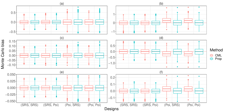
Figure S1: Monte Carlo bias of the proposed and CML estimators based on 1,000 Monte Carlo simulations under the logistic regression model setup. The first to the third rows stand for the Monte Carlo bias for estimating $\beta_{0}$, $\beta_{1}$ and $\beta_{2}$, respectively. The three plots in the left column show the results when the auxiliary variables are independently generated, and those in the right column are for the case when the auxiliaries are dependent. “CML” and “Prop” stands for the CML estimator and the proposed estimator, respectively. The first design in the parenthesis is used to generate the internal sample $\mathcal{S}_{1}$, and the second one to generate the external sample $\mathcal{S}_{2}$. “Poi” represents Poisson sampling.

Web Table S1 shows the coverage rate of a 95% confidence intervals for the proposed estimator under different settings. As in the first simulation, the coverage rats are close to their nominal truth 0.95 under different settings, indicating the satisfactory performance of the proposed estimator.

Table S1: Coverage rate of a 95% confidence interval by the proposed method based on 1,000 Monte Carlo simulations under different setups. “$\mathcal{S}_{1}$ Des” and “$\mathcal{S}_{2}$ Des” show the sampling design used to generate the internal sample $\mathcal{S}_{1}$ and the external sample $\mathcal{S}_{2}$. “SRS” and “Poi” stands for SRS and Poisson sampling, respectively. “Independent” and “Dependent” correspond to the cases when the auxiliary variables are independent and dependent, respectively.

$\mathcal{S}_{1}$ Des	$\mathcal{S}_{2}$ Des	Independent				Dependent
		$\beta_{0}$	$\beta_{1}$	$\beta_{2}$		$\beta_{0}$	$\beta_{1}$	$\beta_{2}$
SRS	SRS	0.963	0.952	0.959		0.957	0.953	0.949
	Poi	0.948	0.955	0.959		0.953	0.954	0.950
Poi	SRS	0.954	0.949	0.940		0.951	0.949	0.946
	Poi	0.941	0.952	0.940		0.952	0.950	0.948

Appendix S4 Validation for the linearity assumption for the KNHANES dataset

For the demonstration purpose, we have assumed two linear regression models in Section 7.3. In this section, we validate the linearity assumption for the regression model.

Figure S2 shows the relationship among the response of interest “Total Cholesterol” and the three covariates. We can conclude that the proposed two linear regression models are reasonable to analyze the KNHANES dataset. Please notice that the KNHANES dataset demonstrates heterogeneity for the linear regression model. Such heterogeneity only influences the efficiency of the proposed method, and it does not invalidate the linear regression model.

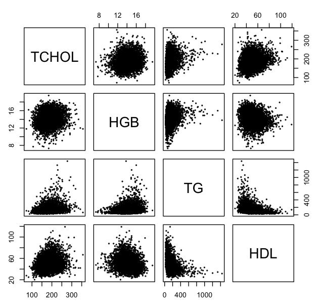
Figure S2: Scatter plots for “Total Cholesterol (TCHOL)”, “Hemoglobin (HGB)”, “Triglyceride (TG)” and “HDL”.

References

• Chatterjee et al. (2016) Chatterjee, N., Y.-H. Chen, P. Maas, and R. Carroll (2016). Constrained maximum likelihood estimation for model calibration using summary-level information from external big data sources. Journal of the American Statistical Association 111, 107–117.
• Chen and Sitter (1999) Chen, J. and R. R. Sitter (1999). A pseudo empirical likelihood approach to the effective use of auxiliary information in complex surveys. Statistica Sinica 9(2), 385–406.
• Chen and Kim (2014) Chen, S. and J. K. Kim (2014). Population empirical likelihood for nonparametric inference in survey sampling. Statistica Sinica 24(1), 335–355.
• Chen et al. (2020) Chen, Y., P. Li, and C. Wu (2020). Doubly robust inference with nonprobability survey samples. Journal of the American Statistical Association 115(532), 2011–2021.
• Chen and Chen (2000) Chen, Y. H. and H. Chen (2000). A unified approach to regression analysis under double-sampling designs. Journal of the Royal Statistical Society: Series B 62, 449–460.
• Csiszár and Shields (2004) Csiszár, I. and P. C. Shields (2004). Information theory and statistics: a tutorial. Foundations and Trands in Communications and Information Theory 1, 417–528.
• Elliott et al. (2017) Elliott, M. R., R. Valliant, et al. (2017). Inference for nonprobability samples. Statistical Science 32(2), 249–264.
• Engle and McFadden (1994) Engle, R. F. and D. L. McFadden (1994). Handbook of Econometrics: Volume IV. Amsterdam.
• Fuller (2009) Fuller, W. A. (2009). Sampling Statistic. Wiley, Hoboken, NJ.
• Han and Lawless (2019) Han, P. and J. F. Lawless (2019). Empirical likelihood estimation using auxiliary summary information with different covariate distributions. Statistica Sinica 29(3), 1321–1342.
• Hansen (1982) Hansen, L. P. (1982). Large sample properties of generalized method of moments estimators. Econometrica 50, 1029–1054.
• Hidiroglou (2001) Hidiroglou, M. (2001). Double sampling. Survey methodology 27, 143–154.
• Horn and Johnson (2012) Horn, R. A. and C. R. Johnson (2012). Matrix Analysis. New York: Cambridge university press.
• Imbens (2002) Imbens, G. W. (2002). Generalized method of moments and empirical likelihood. Journal of Business and Economic Statistics 20, 493–506.
• Kim and Rao (2009) Kim, J. K. and J. N. K. Rao (2009). A unified approach to linearization variance estimation from survey data after imputation for item nonresponse. Biometrika 96, 917–932.
• Kim and Wang (2019) Kim, J. K. and Z. Wang (2019). Sampling techniques for big data analysis in finite population inference. International Statistical Review 87, S177–S191.
• Kundu et al. (2019) Kundu, P., R. Tang, and N. Chatterjee (2019, 07). Generalized meta-analysis for multiple regression models across studies with disparate covariate information. Biometrika 106(3), 567–585.
• Lohr and Raghunathan (2017) Lohr, S. L. and T. E. Raghunathan (2017). Combining survey data with other data sources. Statistical Science 32, 293–312.
• Merkouris (2010) Merkouris, T. (2010). Combining information from multiple surveys by using regression for efficient small domain estimation. Journal of the Royal Statistical Society: Series B 72, 27–48.
• Owen (1991) Owen, A. (1991). Empirical likelihood for linear models. The Annals of Statistics 19, 1725–1747.
• Pfeffermann (1993) Pfeffermann, D. (1993). The role of sampling weights when modeling survey data. International Statistical Review/Revue Internationale de Statistique 61, 317–337.
• Qin and Lawless (1994) Qin, J. and J. Lawless (1994). Empirical likelihood and general estimating equations. The Annals of Statistics 22, 300–325.
• Rao (2021) Rao, J. (2021). On making valid inferences by integrating data from surveys and other sources. Sankhya B 83, 242–272.
• Rivera-Rodriguez et al. (2020) Rivera-Rodriguez, C., S. Haneuse, M. Wang, and D. Spiegelman (2020). Augmented pseudo-likelihood estimation for two-phase studies. Statistical Methods in Medical Research 29, 344–358.
• Rivera-Rodriguez et al. (2019) Rivera-Rodriguez, C., D. Spiegelman, and S. Haneuse (2019). On the analysis of two-phase designs in cluster-correlated data settings. Statistics in Medicine 38, 4611–4624.
• Robins et al. (1994) Robins, J. M., A. Rotnitzky, and L. P. Zhao (1994). Estimation of regression coefficients when some regressors are not always observed. Journal of the American Statistical Association 89, 846–866.
• Sheng et al. (2021) Sheng, Y., Y. Sun, C.-Y. Huang, and M.-O. Kim (2021). Synthesizing external aggregated information in the presence of population heterogeneity: A penalized empirical likelihood approach. Biometrics.
• Sheng et al. (2022) Sheng, Y., Y. Sun, C.-Y. Huang, and M.-O. Kim (2022). Synthesizing external aggregated information in the presence of population heterogeneity: A penalized empirical likelihood approach. Biometrics 78(2), 679–690.
• Shin et al. (2020a) Shin, Y. E., R. M. Pfeiffer, B. I. Graubard, and M. H. Gail (2020a). Weight calibration to improve efficiency for estimating pure risks from the additive hazards model with the nested case-control design. Biometrics Accepted, 1–13.
• Shin et al. (2020b) Shin, Y. E., R. M. Pfeiffer, B. I. Graubard, and M. H. Gail (2020b). Weight calibration to improve the efficiency of pure risk estimates from case-control samples nested in a cohort. Biometrics 76(4), 1087–1097.
• Taylor et al. (2022) Taylor, J. M. G., K. Choi, and P. Han (2022, 04). Data integration: exploiting ratios of parameter estimates from a reduced external model. Biometrika, 1–16. Accepted.
• Wang et al. (1997) Wang, C. Y., S. Wang, L.-P. Zhao, and S.-T. Ou (1997). Weighted semiparametric estimation in regression analysis with missing covariate data. Journal of the American Statistical Association 92, 512–525.
• Wang and Kim (2021) Wang, H. and J. K. Kim (2021). Propensity score estimation using density ratio model under item nonresponse. arXiv preprint arXiv:2104.13469.
• Wang et al. (2020) Wang, L., M. L. Williams, Y. Chen, and J. Chen (2020). Novel two-phase sampling designs for studying binary outcomes. Biometrics 76, 210–223.
• Wu (2005) Wu, C. (2005). Algorithms and R codes for the pseudo empirical likelihood method in survey sampling. Survey Methodology 31, 239.
• Wu and Rao (2006) Wu, C. and J. Rao (2006). Pseudo empirical likelihood ratio confidence intervals for complex surveys. Canadian Journal of Statistics 34, 359–375.
• Wu and Sitter (2001) Wu, C. and R. R. Sitter (2001). A model-calibration approach to using complete auxiliary information from survey data. Journal of the American Statistical Association 96, 185–193.
• Xu and Shao (2020) Xu, M. and J. Shao (2020). Meta-analysis of independent datasets using constrained generalised method of moments. Statistical Theory and Related Fields 4, 109–116.
• Yang and Kim (2020) Yang, S. and J. K. Kim (2020). Statistical data integration in survey sampling: A review. Japanese Journal of Statistics and Data Science 3, 625–650.
• Yang et al. (2020) Yang, S., D. Zheng, and X. Wang (2020). Elastic integrated analysis of randomized trial and real-world data for treatment heterogeneity estimation. arXiv preprint arXiv:2005.10579v2.
• Yuan and Jennrich (1998) Yuan, K.-H. and R. I. Jennrich (1998). Asymptotics of estimating equations under natural conditions. Journal of Multivariate Analysis 65(2), 245–260.
• Zhai and Han (2022) Zhai, Y. and P. Han (2022). Data integration with oracle use of external information from heterogeneous populations. Journal of Computational and Graphical Statistics 0(0), 1–12.
• Zhang et al. (2021) Zhang, H., L. Deng, W. Wheeler, J. Qin, and K. Yu (2021). Integrative analysis of multiple case-control studies. Biometrics Accepted, 1–12.
• Zhao et al. (2020) Zhao, P., M. Ghosh, J. Rao, and C. Wu (2020). Bayesian empirical likelihood inference with complex survey data. Journal of the Royal Statistical Society: Series B 82, 155–174.
• Zubizarreta (2015) Zubizarreta, J. R. (2015). Stable weights that balance covariates for estimation with incomplete outcome data. Journal of the American Statistical Association 110, 910–922.