Semi-Random Impossibilities of Condorcet Criterion

Abstract

The Condorcet criterion (CC) is a classical and well-accepted criterion for voting. Unfortunately, it is incompatible with many other desiderata including participation (Par), half-way monotonicity (HM), Maskin monotonicity (MM), and strategy-proofness (SP). Such incompatibilities are often known as impossibility theorems, and are proved by worst-case analysis. Previous work has investigated the likelihood for these impossibilities to occur under certain models, which are often criticized of being unrealistic.

We strengthen previous work by proving the first set of semi-random impossibilities for voting rules to satisfy CC and the more general, group versions of the four desiderata: for any sufficiently large number of voters $n$, any size of the group $1\leq B\leq\sqrt{n}$, any voting rule $r$, and under a large class of semi-random models that include Impartial Culture, the likelihood for $r$ to satisfy CC and Par, CC and HM, CC and MM, or CC and SP is $1-\Omega(\frac{B}{\sqrt{n}})$. This matches existing lower bounds for C&P ($B=1$) and C&S ($B\leq\sqrt{n}$), showing that many commonly-studied voting rules are already asymptotically optimal in such cases.

1 Introduction

The Condorcet criterion of voting [12] is a classical desideratum that has “nearly universal acceptance” [46, p. 46]. It requires a voting rule to choose the Condorcet winner—the alternative who beats other alternatives in head-to-head competitions—whenever it exists.

Unfortunately, it is well-known that the Condorcet criterion (CC for short) is incompatible with many other desiderata (a.k.a. axioms) when the number of alternatives $m$ is at least $3$. Such incompatibilities are often called impossibility theorems. For example, no voting rule satisfies

• CC and participation (Par for short, which requires that no voter has incentive to abstain from voting), when $m\geq 4$ [36];

• CC and half-way monotonicity (HM for short, which requires that no voter has incentive to reverse his/her vote [47]);

• CC and Maskin monotonicity (MM for short, which requires that any voter raising the position of the winner relative to other alternatives does not change the winner [31]), as a special case of the Muller-Satterthwaite theorem (1977); or

• CC and strategy-proofness (SP for short, which requires that no agent has incentive to lie), as a special case of the Gibbard-Satterthwaite theorem (1973, 1975).

The four combinations of axioms are therefore denoted by C&P, C&H, C&M, and C&S, respectively. Proofs for these impossibility theorems are based on worst-case analysis, by identifying a single instance of violation. Therefore, they do not preclude the possible that such violations are rare in practice. Indeed, if so, “then one need not be unduly worried” [41].

Studying how rare such impossibilities are in practice has been a popular and active field of research [23, 13]. Recently, the topic was investigated using smoothed analysis [50, 3, 53], which can be viewed as a worst average-case analysis under semi-random models [15], following the frequentists’ principle: the likelihood of violation of axioms is estimated under an adversarially chosen (i.e., worst-case) distribution for the votes from a given set of distributions. For example, the likelihood for CC or Par to be violated is $\Theta(\frac{1}{\sqrt{n}})$ for many voting rules for $n$ voters, under a large class of semi-random models [55].

While this is good news, as violations vanish at a $\Theta(\frac{1}{\sqrt{n}})$ rate, they are not rare enough when the cost of violation is high. For example, if a violation of CC or Par leads to a revote, whose social cost is $\Theta(n)$, then the expected social cost is $\Theta({\sqrt{n}})$, which is non-negligible. As another example, if everyone complaints on social media about the violation and gets $-1$ utility every time when seeing a complaint, then the social cost can be as high as $\Theta(n^{2})$, meaning that the expected social cost is $\Omega(n^{1.5})$, or in other words, $\Omega(\sqrt{n})$ per person. In such situations, voting rules with rarer violations are desirable.

But can any voting rule do better, and if so, by how much? The answer lies in the lower bound on the likelihood of violations (under all rules), or equivalently, the upper bound on the likelihood of satisfying the axioms. In this paper, we address this question for the four combinations of axioms involving CC mentioned earlier, by proving semi-random impossibilities [53] under a large class of semi-random models that are more general and realistic than the commonly-used i.i.d. uniform distribution, known as the Impartial Culture (IC). Therefore, the research question of this paper can be phrased as:

What are the semi-random impossibilities of CC?

More precisely, we consider the more general, group versions of $X\in\{\text{\sc C\&P},\text{\sc C\&H},\text{\sc C\&M},\text{\sc C\&S}\}$. For any $B\geq 1$, any collection of votes $P$ (called a profile), and any voting rule $r$, we let ${X}(r,P,B)=1$ if $r$ satisfies CC at $P$ and no group of at most $B$ voters in $P$ can collaboratively violate $X$; otherwise ${X}(r,P,B)=0$. Then, given a set of distributions $\Pi$ over the votes and $n$ agents, the semi-random version of $X$ [53, 55] is defined as:

$$\widetilde{X}_{\Pi}^{\min}(r,n,B)\triangleq\inf\nolimits_{\vec{\pi}\in\Pi^{n}}\Pr\nolimits_{P\sim\vec{\pi}}\left({X}(r,P,B)=1\right)$$ (1)

That is, $\widetilde{X}_{\Pi}^{\min}(r,n,B)$ is the worst-case (lower bound) on the probability for $X$ to be $1$ under the profile $P$ generated from a vector $\vec{\pi}$ of $n$ distributions in $\Pi^{n}$, one for each agent. Notice that while agents’ votes are independently generated, their underlying distributions are adversarially chosen and can be different. A high $\widetilde{X}_{\Pi}^{\min}$ value is desirable, because it implies that the expected satisfaction of $X$ is high even under the worst distribution $\vec{\pi}\in\Pi^{n}$.

1.1 Our Contributions

The main results of this paper are four semi-random impossibility theorems: for $X=\text{\sc C\&P}$ (Theorem 1), C&H (Theorem 2), C&M (Theorem 3), or C&S (Theorem 4), any $m\geq 4$ ($m\geq 3$ for C&M and C&S), any sufficiently large $n$, any $1\leq B\leq\sqrt{n}$, any voting rule $r$, and any $\Pi$ satisfying certain conditions (Assumption 1),

$$\widetilde{X}_{\Pi}^{\min}(r,n,B)=1-\Omega\left(\frac{B}{\sqrt{n}}\right)$$

In other words, no voting rule can guarantee that $X$ is violated with probability smaller than $\Omega(\frac{B}{\sqrt{n}})$. The results also imply that every additional member in the group (up to $\sqrt{n}$) roughly increase the likelihood of violation by $\Theta(\frac{1}{\sqrt{n}})$. Specifically, when $B=\Omega(\sqrt{n})$, the likelihood of violation does not vanish even in large elections ($n\rightarrow\infty$).

Our results match the lower bound for C&P when $B=1$ [55] and for C&S for every $B\leq\sqrt{n}$ [56], which are achieved by many voting rules that satisfies CC, such as Copeland, maximin, ranked pairs, and Schulze—in contrast, for C&P, positional scoring rules and STV are much worst, as their satisfactions are $1-\Theta(1)$ [55].

Good or bad news? On the positive side, it is the first time, to the best of our knowledge, that the optimal likelihood of avoiding impossibility theorems that involve CC is known. It is surprising to us that many existing rules are already optimal. On the negative side, the tightness suggests that there is little room for improvement, which can be a critical concern when the cost of violation is high. After all, we believe that these semi-random impossibility theorems are useful and informative in theory, as they reveal limitations of the optimal rules, as well as in practice, for the decision maker to choose the voting rule and decide the policies when a violation of axioms occurs.

Generality and limitations. The generality of the semi-random impossibilities proved in this paper largely depends on the restrictiveness of Assumption 1. We defer the formal technical definition and discussions to Section 2, and feel that the assumption is mild in practice, because it is satisfied by many single-agent preference models, including IC, the single-agent Mallows and single-agent Plackett-Luce with bounded parameters [53]. As a result, the $1-\Omega(\frac{B}{\sqrt{n}})$ upper bound naturally holds under IC (Corollary 1).

The major limitations are, first, the constant in $\Omega(\frac{B}{\sqrt{n}})$ may be exponentially large in $m$, though it does not depend on $n$, $B$, or $r$. Second, the semi-random model in this paper assumes that the votes are statistically independent (but not necessarily identically distributed). These are common limitations/assumptions in preference modeling, see, e.g., [51, 4, 52]. Addressing them may require breakthroughs in probability theory and are important and challenging directions.

Proof overview.

The high-level idea is surprisingly simple: for each $X$ studied in this paper, in step 1, we leverage existing proof of the (worst-case) impossibility theorem to identify sufficiently many profiles where $X$ is violated. Then, in step 2, we prove that there exists $\vec{\pi}\in\Pi^{n}$ under which with $\Omega(\frac{B}{\sqrt{n}})$ probability, a profile falls in the set identified in step 1.

Nevertheless, the actual calculations are technical challenging due to the generality of $r$. In step 1, we introduce a rotated template by scaling up an existing proof diagram (e.g., [43, Chapter 1]) to identify profiles where $X$ is violated, and prove that there are sufficiently many such violation profiles by upper-bounding the number of times each of them is identified by the rotated template. Then in step 2, we use an averaging argument over all $n!$ permutations of a carefully chosen $\vec{\pi}$ to convert the problem to the likelihood about the histogram of profiles, which is then tackled by applying the point-wise concentration bound [54, Lemma 1].

The idea and techniques have the potential to leverage other (worst-case) impossibility theorems to their semi-random versions. See Section 4 for more discussions.

1.2 Related Work and Discussions

Condorcet criterion (CC) is satisfied by many commonly-studied voting rules. Prominent exceptions are positional scoring rules [19] and multi-round-score-based elimination rules, such as STV. Much previous work aimed at theoretically characterizing the Condorcet efficiency, which is the probability for the Condorcet winner to win conditioned on its existence [18, 17, 40, 22, 39].

Participation (Par) was introduced to study voting rules that avoid the no-show paradox [20]. Moulin [36] proved that when $m\geq 4$ and $n\geq 25$, no voting rule satisfies CC and Par simultaneously. The bound on $n$ was characterized to be $12$ by simplified, SAT-solver-based proofs [9, 43]. The likelihood of Par satisfaction by popular voting rules under IC was investigated in a series of work as summarized by Gehrlein and Lepelley [23, Chapter 4.2.2], and also more recently by Brandt et al. [10].

Half-way monotonicity (HM) was introduced to study voting rules that avoid the preference reversal paradox, and was proved to be incompatible with CC [47]. Peters [42] used SAT solvers to characterized the number of voters under which the impossibility holds.

Maskin monotonicity (MM) was introduced to characterize Nash implementability [31]. The Muller-Satterthwaite theorem [37] establishes the equivalence between MM and SP in the worst-case sense: a voting rule satisfies MM if and only if it satisfies SP.

Strategy-proofness (SP) cannot be satisfied by any non-dictatorial and unanimous voting rules when $m\geq 3$, due to the Gibbard-Satterthwaite theorem [24, 48]. SP is stronger than HM, because the latter uses a special form of manipulation (by reversing the truthful vote). At a high-level, Par can be viewed as a weak form of SP that prevents manipulation by abstention, though Par is not weaker than SP by definition, because Par reasons about elections of different sizes. A quantitative Gibbard-Satterthwaite theorem (under IC) was proved for $m=3$ by Friedgut et al. [21], and was subsequently developed in [14, 57, 25], and the case for general $m$ was resolved by Mossel and Racz [33].

Semi-random C&P, C&H, C&M, and C&S. We are not aware of any semi-random impossibility theorem about the satisfaction of C&P, C&H, or C&M, even under IC. For SP, the quantitative Gibbard-Satterthwaite theorem by Mossel and Racz [33] establishes an $1-\Omega(\frac{1}{n^{67}})$ upper bound under IC for any voting rule that is sufficiently different from dictatorships. Therefore, the same bound holds for C&S for any rule that satisfies CC. The $1-\Omega(\frac{B}{\sqrt{n}})$ upper bound for C&S in our Theorem 4 also applies to all CC rules, which is stronger than the special case of [33], because our bound is lower and works for every $B\leq\sqrt{n}$ under more general models.

For possibility results (i.e., lower bound for optimal rules), as discussed in Section 1.1, our results imply that the bounds are tight for C&P (when $B=1$) and for C&S (when $B\leq\sqrt{n}$). We conjecture that they are tight for other axioms studied in this paper with all $B\leq\sqrt{n}$.

Quantitative and semi-random impossibilities. There is a large body of literature on quantitative impossibility theorems in social choice under IC. For example, quantitative versions of Arrow’s impossibility theorem [1] were proved [26, 32, 27, 34]. In judgement aggregation, Nehama [38] and Filmus et al. [16] developed quantitative characterizations of AND-homomorphism as oligarchy, whose worst-case version was due to List and Pettit [28, 29]. Xia [53] proved a semi-random version of the ANR impossibility theorem on anonymity and neutrality, whose worst-case version was proved by Moulin [35].

Other smoothed/semi-random results. Semi-random models have been widely adopted to analyze the performance of algorithms in practice in combinatorial optimization [7], mathematical programming [49], machine learning [5], and algorithmic game theory [11, 44, 8, 6], etc. We refer the readers to recent surveys on semi-random models [15] and general approaches beyond worst-case analysis [45]. In addition to the work discussed above, semi-random/smoothed analysis has been applied to other social choice problems, e.g., likelihood of ties [54], complexity of winner determination [58], judgement aggregation [30], and fair division [2].

2 Preliminaries

For any $q\in\mathbb{N}$, we let $[q]=\{1,\ldots,q\}$. Let $\mathcal{A}=[m]$ denote the set of $m\geq 3$ alternatives. Let $\mathcal{L}(\mathcal{A})$ denote the set of all linear orders over $\mathcal{A}$. Let $n\in\mathbb{N}$ denote the number of voters (agents). Each voter uses a linear order $R\in\mathcal{L}(\mathcal{A})$ to represent his or her preferences, called a vote, where $a\succ_{R}b$ means that the agent prefers alternative $a$ to alternative $b$. The vector of $n$ voters’ votes, denoted by $P$, is called a (preference) profile, sometimes called an $n$-profile. A voting rule $r$ maps any profile to a single winner. For any profile $P$, let $\text{Hist}(P)\in{\mathbb{R}}_{\geq 0}^{m!}$ denote the anonymized version of $P$, also called the histogram of $P$, which contains the total number of each linear order in $\mathcal{L}(\mathcal{A})$ according to $P$.

Weighted majority graphs and the Condorcet winner. For any profile $P$ and any pair of alternatives $(a,b)$, let $P[a\succ b]$ denote the number of votes in $P$ where $a$ is preferred to $b$. Let $\text{WMG}(P)$ denote the weighted majority graph of $P$, whose vertices are $\mathcal{A}$ and whose weight on edge $a\rightarrow b$ is $w_{P}(a,b)=P[a\succ b]-P[b\succ a]$. The Condorcet winner of a profile $P$ is the alternative whose outgoing edges in $\text{WMG}(P)$ are positively weighted.

Condorcet criterion. All axioms studied in this paper are per-profile axioms [53], each of which is modeled as a function ${X}$ that maps a voting rule $r$, a profile $P$, and a group size $B\geq 1$ to $\{0,1\}$, where $0$ (respectively $1$) means that $r$ violates (respectively, satisfies) the axiom at $P$ w.r.t. group size $B$. Then, the classical (worst-case) satisfaction of the axiom under $r$ becomes $\min_{P}{X}(r,P)$.

For any voting rule, any profile $P$, and any $B\geq 1$, Condorcet criterion is modeled as a function CC such that ${\text{\sc CC}}(r,P,B)=1$ if and only if either (1) there is no Condorcet winner under $P$, or (2) the Condorcet winner is the winner of $P$ under $r$. Notice that technically CC does not depend on $B$, which is included for notational consistency.

Participation is modeled by a function Par such that ${\text{\sc Par}}(r,P,B)=1$ if and only if no group of at most $B$ voters have incentive to abstain from voting; otherwise ${\text{\sc Par}}(r,P,B)=0$. Formally, ${\text{\sc Par}}(r,P,B)=0$ if and only if there exists a subvector $P^{\prime}$ of $P$ such that for all $R\in P^{\prime}$, $r(P^{\prime})\succ_{R}r(P)$. The simultaneous satisfaction of CC and Par is denoted by C&P, such that ${\text{\sc C\&P}}(r,P,B)=1$ if and only if ${\text{\sc CC}}(r,P,B)=1$ and ${\text{\sc Par}}(r,P,B)=1$.

Half-way monotonicity is modeled by a function HM such that ${\text{\sc HM}}(r,P,B)=1$ if and only if no coalition of at most $B$ voter have incentive to flip their votes so that the outcome is more preferred to each of them; otherwise ${\text{\sc Par}}(r,P,B)=0$.

Maskin monotonicity is modeled by a function MM such that ${\text{\sc MM}}(r,P,B)=1$ if and only if whenever no more than $B$ voters raise the position of the current winner relative to other alternatives, the winner stays the same; otherwise ${\text{\sc MM}}(r,P,B)=0$. More precisely, given two rankings $R_{1},R_{2}\in\mathcal{L}(\mathcal{A})$ and an alternative $a$, we say that the position of $a$ is raised in $R_{2}$ relative to other alternatives from $R_{1}$ if and only if the set of alternatives $a$ is preferred to in $R_{1}$ is a subset of the set of alternatives $a$ is preferred to in $R_{2}$, i.e.,

$$\{b:a\succ_{R_{1}}b\}\subseteq\{b:a\succ_{R_{2}}b\}$$

Notice that the inclusion does not need to be strict. That is, if the the set of alternatives $a$ is preferred to is unchanged, then we still say that the position of $a$ is raised in $R_{2}$ relative to other alternatives.

Strategy-proofness is modeled by a function SP such that ${\text{\sc SP}}(r,P,B)=1$ if and only if no coalition of at most $B$ voter have incentive to change their votes so that the outcome is more preferred to each of them; otherwise ${\text{\sc SP}}(r,P,B)=0$.

Group versions of the axioms. For any $X\in\{\text{\sc Par},\text{\sc HM},\text{\sc MM},\text{\sc SP}\}$, if ${X}(r,P,B)=1$, then we also say that $P$ satisfies $X_{B}$.

Proof diagram of the C&P impossibility. We briefly recall the proof diagram by Peters [43, Chapter 1] in Figure 1 to show that when $m=4$, no voting rule $r$ satisfies C&P, which will play an important role in our proofs later. Each edge represents a sequence of operations, conditioned on the winner of the source profile being highlighted. Peters [43, Chapter 1] proved that a violation of CC and/or Par exists in the diagram. Take the leftmost branch for example. If $r(P_{0})\in\{1,2\}$, then two copies of $[1234]$ are added one by one. If the winner is no longer $1$ or $2$ during this process, then Par is violated. Otherwise, starting from $P_{\{1,2\}}$, if $r(P_{\{1,2\}})=\{1\}$, then three votes of $[2431]$ are subtracted one by one. If the winner is not $1$ at any point, then Par is violated. However,$3$ is the Condorcet winner in the leaf node, which means that CC is violated if Par has not been violated on the leftmost branch so far.

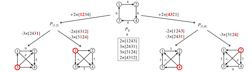
Figure 1: Proof diagram of C&P impossibility [43, Chapter 1]. WMGs of the root and the leaves are shown (where all unweighted edges in the leaves have weight $1$). Each edge represents a sequence of operations conditioned on the winner of the source profile being a highlighted alternative. Condorcet winners in the leaf nodes are highlighted.

Semi-random satisfaction of axioms. Given a per-profile axiom $X$, a set $\Pi$ of distributions over $\mathcal{L}(\mathcal{A})$, a voting rule $r$, $n\in\mathbb{N}$, and a group size $B$, the semi-random satisfaction of $X$ under $r$ with $n$ agents, denoted by $\widetilde{X}_{\Pi}^{\min}(r,n,B)$, is defined in Equation (1) in the Introduction. The “min” in the superscript means that the adversary aims at minimizing the satisfaction of $X$.

The semi-random analysis generalizes the classical quantitative analysis in social choice (under IC). To see this, let ${\pi}_{\text{uni}}$ denote the uniform distribution over $\mathcal{L}(\mathcal{A})$ and let $\Pi_{\text{IC}}=\{{\pi}_{\text{uni}}\}$. Then, $\widetilde{X}_{\Pi_{\text{IC}}}^{\min}$ becomes the likelihood of satisfaction of $X$ under IC. Throughout the paper, we make the following assumptions on $\Pi$.

Assumption 1

We assume that $\Pi$ is

• strictly positive, which means that there exists $\epsilon>0$ such that for every $\pi\in\Pi$ and every $R\in\mathcal{L}(\mathcal{A})$, $\pi(R)\geq\epsilon$;

• closed, which means that $\Pi$ is a closed subset of the probability simplex in $\mathbb{R}^{m!}$; and

• ${\pi}_{\text{uni}}\in\text{CH}(\Pi)$, where $\text{CH}(\Pi)$ is the convex hull of $\Pi$.

The first part of Assumption 1 requires that no distribution in $\Pi$ is too “deterministic”. The second part is a mild technical assumption. The first two parts guarantee that the semi-random analysis using $\Pi$ is sufficiently different from the worst-case analysis. The third part requires that the uniform distribution ${\pi}_{\text{uni}}$ is in the convex hull of $\Pi$, though ${\pi}_{\text{uni}}$ itself may not be in $\Pi$.

We believe that Assumption 1 is mild, because it is satisfied by many classical models for preferences. For example, it is satisfied by IC, which corresponds to $\Pi=\{{\pi}_{\text{uni}}\}$. The following example is taken from [53].

Example 1

In the single-agent Mallows with bounded dispersion, given $\underline{\varphi}>0$, each distribution is parameterized by a central ranking $W\in\mathcal{L}(\mathcal{A})$ and a dispersion $\varphi\in[\underline{\varphi},1]$, such that the probability for $R\in\mathcal{L}(\mathcal{A})$ is proportional to $\varphi^{\text{KT}(R,W)}$, where $\text{KT}(R,W)$ is the total number of pairwise differences between $R$ and $W$, i.e., the Kendall-Tau distance.

In the single-agent Plackett-Luce with bounded parameters, given $\underline{\varphi}>0$, each distribution is parameterized by a vector $\vec{\theta}\in[\underline{\varphi},1]^{m}$ such that $\vec{\theta}\cdot\vec{1}=1$. The probability for $R=a_{1}\succ a_{2}\succ\cdots\succ a_{m}$ is $\prod_{i=1}^{m-1}({\theta_{a_{i}}}/{\sum_{\ell=i}^{m}\theta_{a_{\ell}}})$.

For any $\underline{\varphi}>0$, both models in the example satisfy Assumption 1.

If $\underline{\varphi}=0$ is allowed in Example 1, then the semi-random analysis degenerates to worst-case analysis, which trivializes the question.

3 Semi-Random Impossibility of CC and Par

Theorem 1 (CC+Participation)

For any fixed $m\geq 4$, any $\Pi$ that satisfies Assumption 1, any voting rule $r$, any $n\geq 12$, and any $1\leq B\leq\sqrt{n}$,

$$\widetilde{\text{\sc C\&P}}_{\Pi}^{\min}(r,n,B)=1-\Omega\left(\frac{B}{\sqrt{n}}\right)$$

The theorem is more general than its classical, worst-case counterpart, as the likelihood is strictly smaller than $1$. It is also more general than its quantitative counterparts (under IC), because the latter is a special case of the former, where $\Pi=\{{\pi}_{\text{uni}}\}$, as discussed in the last section.

Proof: To illustrate the idea, we make the following assumptions in the proof sketch: (i) $m=4$, (ii) $\sqrt{n}$ is an integer, (iii) $B\mid\sqrt{n}$, and (iv) $m!\mid n$. Then, we modify the proof for the general case. It suffices to prove the theorem when $n\geq 12$ and is sufficiently large, because the (worst-case) impossibility theorem holds for every $n\geq 12$ [9, 43].

Overview. Let $\text{\sc Par}_{B}$ denote the group version of participation with size $B$. Instead of upper-bounding $\widetilde{\text{\sc C\&P}}_{\Pi}^{\min}$, we will lower-bound its complement $\widetilde{\neg(\text{\sc C\&P})}_{\Pi}^{\max}$ as $\Omega(\frac{B}{\sqrt{n}})$, which is the max-semi-random likelihood for CC or $\text{\sc Par}_{B}$ to be violated and is defined similarly to $\widetilde{X}_{\Pi}^{\min}$ in (1), except that $\inf$ is replaced by $\sup$. The theorem then follows after noticing

$$\widetilde{\text{\sc C\&P}}_{\Pi}^{\min}(r,n,B)=1-\widetilde{\neg(\text{\sc C\&P})}_{\Pi}^{\max}(r,n,B)$$

As discussed in Section 1.1, the proof proceeds in two steps. In step 1, we identify a set of $n$-profiles, denoted by $\mathcal{V}_{n,B}$, where CC or $\text{\sc Par}_{B}$ is violated, and prove that $\mathcal{V}_{n,B}$ contains sufficiently many profiles. This will be achieved by first scaling the (worst-case) proof diagram in [43, Chapter 1], i.e., Figure 1 in Section 2, by a factor of $\sqrt{n}$ to define a violation template, and then implementing it at profiles whose histograms are in an $O(\sqrt{n})$ neighborhood of $\frac{n}{m!}\cdot\vec{1}$. Each implementation leads to a violation tree, which contains at least one violation of CC or $\text{\sc Par}_{B}$. Then, we upper-bound the number of violation trees any profile $P^{*}\in\mathcal{V}_{n,B}$ can be on, by considering the rotated trees generated by the rotated template rooted at $P^{*}$.

Then in step 2, we prove that there exists $\vec{\pi}\in\Pi^{n}$ so that the likelihood of $\mathcal{V}_{n,B}$ found in step 1 is lower-bounded by $\Omega(\frac{B}{\sqrt{n}})$. This is achieved by starting with a $\vec{\pi}\in\Pi^{n}$ such that $\sum_{j=1}^{n}\pi_{j}$ is $O(1)$ away from $\frac{n}{m!}\cdot\vec{1}$, and then considering the sum of likelihood of $\mathcal{V}_{n,B}$ under all $n!$ permutations of components in $\vec{\pi}$. This converts the likelihood of $\mathcal{V}_{n,B}$ to the likelihood about the histogram of a randomly-generated profile. Finally, we apply the point-wise concentration bound [54, Lemma 1] to derive the desired lower bound.

Step 1. We first formally define the violation template illustrated in Figure 2.

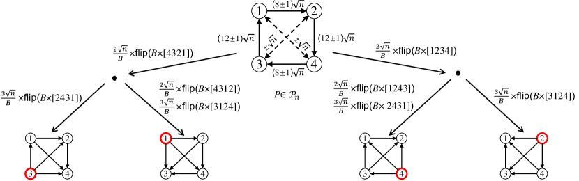
Figure 2: The violation template. “$\pm$” represents the upper and lower bounds on the weight. $\ell\times\text{\rm flip}(B\times R)$ represents $\ell$ operations, each of which flips $B$ votes that are $R$. In the leaves, weights are not shown and Condorcet winners are highlighted.

Definition 1 (Violation template)

Given any $n$-profile $P$ with at least $7\sqrt{n}$ copies of $\mathcal{L}(\mathcal{A})$ and any $1\leq B\leq\sqrt{n}$, a violation template is defined by modifying the proof diagram (Figure 1) as follows, where ${\text{Rev}\left(R\right)}$ denote the reverse ranking of $R$:

• every $+R$ operation on an edge in Figure 1 is replaced by a sequence of $\frac{\sqrt{n}}{B}$ operations, each of which flips $B\times{\text{Rev}\left(R\right)}$ votes and is denoted by ${\text{\rm flip}}({B\times{\text{Rev}\left(R\right)})}$;

• every $-R$ operation on an edge in Figure 1 is replaced by a sequence of $\frac{\sqrt{n}}{B}$ operations, each of which flips $B\times R$ votes and is denoted by ${\text{\rm flip}}({B\times R)}$.

The violation template will be implemented multiple times, by letting its root to be $n$-profiles whose WMGs are similar to the WMG at the root in Figure 1 (scaled by a factor of $\sqrt{n}$) and whose histograms are close to $\frac{n}{m!}\cdot\vec{1}$. Formally, we define the set of such profiles $P$, denoted by $\mathcal{P}_{n}$, as follows. Let $w(e)$ denote the weight on edge $e$ in the root of Figure 1.

Definition 2

Let $\mathcal{P}_{n}$ denote the set of $n$-profiles $P$ such that

• for every edge $e\in[4]\times[4]$, $|w_{P}(e)-\sqrt{n}\cdot w(e)|\leq\sqrt{n}$;

• $|\text{Hist}(P)-\frac{n}{m!}\cdot\vec{1}|_{\infty}\leq 4\sqrt{n}$.

We note that any flip operation in the violation template does not completely specify the set of voters whose votes should be flipped (except that their votes must be the same as the designated ranking). Consequently, different combinations of votes when implementing the violation template lead to different violation trees, formally defined as follows.

Definition 3 (Violation trees)

For any $P\in\mathcal{P}_{n}$ and any $1\leq B\leq\sqrt{n}$, a violation tree is a tree of $\frac{20\sqrt{n}}{B}+1$ profiles obtained from implementing the violation template rooted at $P$. Let $\mathcal{T}_{P,B}$ denote the set of all violation trees rooted at $P$.

For example, in a violation tree rooted at $P\in\mathcal{P}_{n}$, the left branch of Figure 2 contains $\frac{5\sqrt{n}}{B}+1$ profiles. The first profile is $P$, and each of the following $\frac{2\sqrt{n}}{B}$ profiles are obtained from the previous one by flipping $B$ votes of $[4321]$. Then, the branch continues with $\frac{3\sqrt{n}}{B}$ profiles, each of which is obtained from the previous profile by flipping $B$ votes of $[2431]$. The following claim lower-bounds the size of $\mathcal{T}_{P,B}$.

Claim 1

For any $P\in\mathcal{P}_{n}$ and any $1\leq B\leq\sqrt{n}$, $|\mathcal{T}_{P,B}|=\Omega\left(\left(\frac{n}{m!\sqrt[B]{B!}}\right)^{20\sqrt{n}}\right)$.

Proof: For any profile $P^{\prime}$ on any violation tree in $\mathcal{T}_{P,B}$, $\text{Hist}(P^{\prime})$ is in the $7\sqrt{n}$ neighborhood of $\frac{n}{m!}\cdot\vec{1}$ in $L_{\infty}$. For any operation $\text{flip}(B\times R)$, let $n_{R}$ denote the number of $R$ votes in $P^{\prime}$. Then, the number of combinations of $B$ votes, each of which being $R$, is ${n_{R}\choose B}$, which is at least $\frac{(\frac{n}{m!}-8\sqrt{n})^{B}}{B!}$. Because the total number of operations in a violation template is $\frac{20\sqrt{n}}{B}$, for any sufficiently large $n$, the total number of violation trees rooted at $P^{\prime}$ is at least

$$\left(\frac{(\frac{n}{m!}-8\sqrt{n})^{B}}{B!}\right)^{\frac{20\sqrt{n}}{B}}$$

$$= \left(\frac{n}{m!\sqrt[B]{B!}}\right)^{20\sqrt{n}}\cdot\left(1-\frac{8m!}{\sqrt{n}}\right)^{20\sqrt{n}}$$

$$= \Omega\left(\left(\frac{n}{m!\sqrt[B]{B!}}\right)^{20\sqrt{n}}\right)$$

$\Box$

The next claim states that each violation tree contains a violation of CC or $\text{\sc Par}_{B}$.

Claim 2

For every $P\in\mathcal{P}_{n}$ and every $T\in\mathcal{T}_{P,B}$, CC or $\text{\sc Par}_{B}$ is violated in $T$.

Proof: Following the proof diagram by [43, Chapter 1] (also see Section 2 and Figure 1), there exists a pair of profiles $P_{1},P_{2}$ in $T$ such that $P_{2}$ is obtained from $P_{1}$ by an operation, which flips $B$ votes of $R$, and either $P_{2}$ violates CC or $r(P_{2})\succ_{R}r(P_{1})$. If $P_{2}$ violates CC then the claim automatically holds. Otherwise, we have $r(P_{2})\succ_{R}r(P_{1})$. Let $\{n_{1},n_{2},\ldots,n_{B}\}\subseteq[n]$ denote the indices to the flipped votes in $P_{1}$ in order to reach $P_{2}$. For every $1\leq t\leq B$, let $P_{1}^{t}$ (respectively, $P_{2}^{t}$) denote the $(n-t)$-profile that is obtained from $P_{1}$ (respectively, $P_{2}$) by removing voters $\{n_{1},\ldots,n_{t}\}$. It follows that $P_{1}^{B}=P_{2}^{B}$. Then, there are two cases.

• If $r(P_{1}^{B})\succ_{R}r(P_{1})$, then $\text{\sc Par}_{B}$ is violated at $P_{1}$, because the $B$ voters $\{n_{1},\ldots,n_{B}\}$ can improve the winner by abstaining from voting.

• Otherwise, because $r(P_{2})\succ_{R}r(P_{1})$, we have $r(P_{2})\succ_{R}r(P_{1}^{B})=r(P_{2}^{B})$, which means that $r(P_{2}^{B})\succ_{{\text{Rev}\left(R\right)}}r(P_{2})$. Therefore, $\text{\sc Par}_{B}$ is violated at $P_{2}$, because the $B$ voters $\{n_{1},\ldots,n_{B}\}$, whose votes are ${\text{Rev}\left(R\right)}$, can improve the winner by abstaining from voting.

In both cases CC and/or $\text{\sc Par}_{B}$ is violated at a profile in $T$, which proves Claim 2. $\Box$

Let $\mathcal{V}_{n,B}$ denote the set of all profiles on violation trees $\bigcup_{P\in\mathcal{P}_{n}}\mathcal{T}_{P,B}$, where CC or $\text{\sc Par}_{B}$ is violated. The next claim upper-bounds the number of violation trees that each profile in $\mathcal{V}_{n,B}$ can possibly be on.

Claim 3

Every $P^{*}\in\mathcal{V}_{n,B}$ is on no more than $O\left(\frac{\sqrt{n}}{B}\cdot\left(\frac{n}{m!\sqrt[B]{B!}}\right)^{20\sqrt{n}}\right)$ violation trees rooted in $\mathcal{P}_{n}$.

Proof: For every node $V$ in the violation template, we define a rotated template, which reverses all edges along the path from the root to $V$. That is, an edge $V_{1}\rightarrow V_{2}$ along the path that flips $B\times R$ becomes $V_{1}\leftarrow V_{2}$ in the rotated template that flips $B\times{\text{Rev}\left(R\right)}$. Consequently, the rotated template is a diagram rooted at $V$. Because each violation template has $\frac{20\sqrt{n}}{B}+1$ nodes, there are $\frac{20\sqrt{n}}{B}+1$ rotated templates. Figure 3 illustrates a rotated template rooted at a node in the leftmost branch.

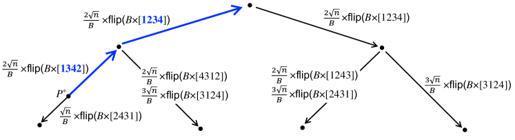
Figure 3: A rotated template rooted at $P^{*}$. Reversed edges and rankings are highlighted.

Like the violation templates, any rotated template leads to rotated trees rooted at any profile $P^{*}$ that contains sufficiently many copies of $\mathcal{L}(\mathcal{A})$. Given a rotated template and $P^{*}\in\mathcal{V}_{n,B}$, because violation trees are rooted at profiles in $P_{n}$, and each node in a violation tree is obtained from the root by modifying no more than $7\sqrt{n}$ votes, we have $|\text{Hist}(P^{*})-\frac{n}{m!}\cdot\vec{1}|\leq 11\sqrt{n}$. This means that the histogram of any profile on the rotated tree is no more than $18\sqrt{n}$ away from $\frac{n}{m!}\cdot\vec{1}$. Therefore, like the proof of Claim 1, the number of rotated trees rooted at $P^{*}$ is at most

$$\left(\frac{(\frac{n}{m!}+18\sqrt{n})^{B}}{B!}\right)^{\frac{20\sqrt{n}}{B}}$$

$$= \left(\frac{n}{m!\sqrt[B]{B!}}\right)^{20\sqrt{n}}\cdot\left(1+\frac{18m!}{\sqrt{n}}\right)^{20\sqrt{n}}$$

$$= O\left(\left(\frac{n}{m!\sqrt[B]{B!}}\right)^{20\sqrt{n}}\right)$$

Because there are $\frac{20\sqrt{n}}{B}+1$ rotated templates and each violation tree that contains $P^{*}$ is equivalent to a rotated tree rooted at $P^{*}$, the number of violation trees that contains $P^{*}$ is no more than

$$\left(\frac{20\sqrt{n}}{B}+1\right)\cdot O\left(\left(\frac{n}{m!\sqrt[B]{B!}}\right)^{20\sqrt{n}}\right)$$

$$= O\left(\frac{\sqrt{n}}{B}\cdot\left(\frac{n}{m!\sqrt[B]{B!}}\right)^{20\sqrt{n}}\right)$$

This completes the proof of Claim 3. $\Box$

We are now ready to lower-bound $|\mathcal{V}_{n,B}|$. To this end, we count the number of (profile, violation tree) pairs, denoted by $(P,T)$, where $T$ is rooted at a profile in $\mathcal{P}_{n}$, $P$ is on $T$, and CC and/or $\text{\sc Par}_{B}$ is violated at $P$. By Claim 1 and Claim 2, the total number of such (profile, violation tree) pairs is at least $|\mathcal{P}_{n}|\times\Omega\left(\left(\frac{n}{m!\sqrt[B]{B!}}\right)^{20\sqrt{n}}\right)$. By Claim 3, the total number of such (profile, violation tree) pairs is at most $|\mathcal{V}_{n,B}|\times O\left(\frac{\sqrt{n}}{B}\cdot\left(\frac{n}{m!\sqrt[B]{B!}}\right)^{20\sqrt{n}}\right)$. Therefore,

$$\frac{|\mathcal{V}_{n,B}|}{|\mathcal{P}_{n}|}\geq\frac{\Omega\left(\left(\frac{n}{m!\sqrt[B]{B!}}\right)^{20\sqrt{n}}\right)}{O\left(\frac{\sqrt{n}}{B}\cdot\left(\frac{n}{m!\sqrt[B]{B!}}\right)^{20\sqrt{n}}\right)}=\Omega\left(\frac{B}{\sqrt{n}}\right)$$ (2)

Step 2. Let $\vec{\pi}\in\Pi^{n}$ be such that $\sum_{j=1}^{n}\pi_{j}$ is $O(1)$ away from $\frac{n}{m!}\cdot\vec{1}$, which can be defined by rounding as shown in [54]. Let $\mathcal{S}_{n}$ denote the set of all permutations over $[n]$. For any permutation $\eta\in\mathcal{S}_{n}$, let $\eta(\vec{\pi})$ denote the vector of distributions where the indices are permuted according to $\eta$. That is, $\eta(\vec{\pi})=(\pi_{\eta(1)},\ldots,\pi_{\eta(n)})$. We prove that there exists a permutation $\eta$ over $[n]$, such that

$$\Pr\nolimits_{P\sim\eta(\vec{\pi})}(P\in\mathcal{V}_{n,B})=\Omega\left(\frac{B}{\sqrt{n}}\right)$$ (3)

It suffices to prove that the sum of the left hand side of (3) for all $\eta\in\mathcal{S}_{n}$ is at least $n!$ times the right hand side of (3), that is,

$$\sum\nolimits_{\eta\in\mathcal{S}_{n}}\Pr\nolimits_{P\sim\eta(\vec{\pi})}(P\in\mathcal{V}_{n,B})=\Omega\left(n!\cdot\frac{B}{\sqrt{n}}\right)$$ (4)

Nevertheless, (4) is still hard to prove due to the lack of information about the profiles in $\mathcal{V}_{n,B}$. The key insight of our proof is to convert the left hand side of (4) to probabilities for the histogram of $P$ to be the histograms of profiles in $\mathcal{V}_{n,B}$. Notice that the left hand side of (4) is equivalent to

$$\sum\nolimits_{\eta\in\mathcal{S}_{n}}\sum\nolimits_{P^{*}\in\mathcal{V}_{n,B}}\Pr\nolimits_{P\sim\eta(\vec{\pi})}(P=P^{*})$$

$$= \sum\nolimits_{P^{*}\in\mathcal{V}_{n,B}}\sum\nolimits_{\eta\in\mathcal{S}_{n}}\Pr\nolimits_{P\sim\vec{\pi}}(P=\eta^{-1}(P^{*}))$$

$$= \sum\nolimits_{P^{*}\in\mathcal{V}_{n,B}}\sum\nolimits_{\eta\in\mathcal{S}_{n}}\Pr\nolimits_{P\sim\vec{\pi}}(P=\eta^{-1}(P^{*}))$$

$$= \sum\nolimits_{P^{*}\in\mathcal{V}_{n,B}}\prod\nolimits_{R\in\mathcal{L}(\mathcal{A})}(n^{*}_{R}!)\times$$

$$\hskip 48.36967pt\Pr\nolimits_{P\sim\vec{\pi}}(\text{Hist}(P)=\text{Hist}(P^{*})),$$ (5)

where $n^{*}_{R}$ is the number of $R$ votes in $P^{*}$. (5) follows the following claim.

Claim 4

For any $P^{*}\in\mathcal{V}_{n,B}$,

$$\sum\nolimits_{\eta\in\mathcal{S}_{n}}\Pr\nolimits_{P\sim\vec{\pi}}(P=\eta^{-1}(P^{*}))=\prod\nolimits_{R\in\mathcal{L}(\mathcal{A})}(n^{*}_{R}!)\times\Pr\nolimits_{P\sim\vec{\pi}}(\text{Hist}(P)=\text{Hist}(P^{*}))$$

Proof: Let $M$ (respectively, $\hat{M}$) denote the set (respectively, multi-set) of $n$-profiles $\{\eta^{-1}(P^{*}):\eta\in\mathcal{S}_{n}\}$. It follows that $\hat{M}$ consists of $\prod\nolimits_{R\in\mathcal{L}(\mathcal{A})}(n^{*}_{R}!)$ copies of $M$. Therefore,

$$\sum\nolimits_{\eta\in\mathcal{S}_{n}}\Pr\nolimits_{P\sim\vec{\pi}}(P=\eta^{-1}(P^{*}))$$

$$= \sum\nolimits_{P^{\prime}\in\hat{M}}\Pr\nolimits_{P\sim\vec{\pi}}(P=P^{\prime})$$

$$= \prod\nolimits_{R\in\mathcal{L}(\mathcal{A})}(n^{*}_{R}!)\sum\nolimits_{P^{\prime}\in M}\Pr\nolimits_{P\sim\vec{\pi}}(P=P^{\prime})$$

$$= \prod\nolimits_{R\in\mathcal{L}(\mathcal{A})}(n^{*}_{R}!)\Pr\nolimits_{P\sim\vec{\pi}}(\text{Hist}(P)=\text{Hist}(P^{*})),$$

which proves the claim. $\Box$

Because $\text{Hist}(P^{*})$ is $7\sqrt{n}$ away from $\frac{n}{m!}\cdot\vec{1}$, we have $\prod\nolimits_{R\in\mathcal{L}(\mathcal{A})}(n^{*}_{R}!)=\Theta\left(\left(\frac{n}{m!}\right)!\right)$. By the point-wise concentration lemma [54, Lemma 1], the likelihood for the histogram of $P$ to be any $\vec{x}$ in an $O(\sqrt{n})$ neighborhood of $\sum_{j=1}^{n}\pi_{j}$ is $\Omega(n^{(1-m!)/2})$. Recall that $\sum_{j=1}^{n}\pi_{j}$ is $O(1)$ away from $\frac{n}{m!}\cdot\vec{1}$. Therefore, for every $P^{*}\in\mathcal{V}_{n,B}$,

$$\Pr\nolimits_{P\sim\vec{\pi}}(\text{Hist}(P)=\text{Hist}(P^{*}))=\Omega\left(n^{(1-m!)/2}\right)$$ (6)

Combining (2), (5), and (6), the left hand side of (4) becomes

$$\Omega\left(|\mathcal{V}_{n,B}|\cdot\left(\frac{n}{m!}\right)!\cdot n^{(1-m!)/2}\right)$$

$$= \Omega\left(\frac{B}{\sqrt{n}}\cdot\left(\frac{n}{m!}\right)!\cdot|\mathcal{P}_{n}|\cdot n^{(1-m!)/2}\right)$$ (7)

Next, we lower-bound $|\mathcal{P}_{n}|$ in the following claim.

Claim 5

$|\mathcal{P}_{n}|=\Omega\left(\frac{n!}{\left(\frac{n}{m!}\right)!}\cdot n^{(m!-1)/2}\right)$.

Proof: Let $P$ denote the $n$-profile obtained from any profile whose histogram is $\frac{n}{m!}\cdot\vec{1}$ by flipping $2\sqrt{n}\times[1234]$, $3\sqrt{n}\times[2431]$, $3\sqrt{n}\times[3124]$, and $2\sqrt{n}\times[4312]$. Then, we have $P\in\mathcal{P}_{n}$. Moreover, let $\mathcal{N}$ denote the set of $n$-profiles whose histograms are no more than $\frac{\sqrt{n}}{m!}$ away from $\text{Hist}(P)$ in $L_{\infty}$. It follows that $\mathcal{N}\subseteq\mathcal{P}_{n}$ and the histogram of any profile in $\mathcal{P}_{n}$ is no more than $\frac{4\sqrt{n}}{m!}$ away from $\frac{n}{m!}\cdot\vec{1}$. Therefore,

$$|\mathcal{P}_{n}|\geq|\mathcal{N}|\geq \left(\frac{\sqrt{n}}{m!}\right)^{m!-1}\times\frac{n!}{\left(\frac{n}{m!}+4\sqrt{n}\right)^{m!}}$$

$$= \Omega\left(\left(\sqrt{n}\right)^{(m!-1)/2}\right)\times\Omega\left(\frac{n!}{\left(\frac{n}{m!}\right)^{m!}}\right),$$

where $\left(\frac{\sqrt{n}}{m!}\right)^{m!-1}$ is a lower bound on the number of histograms in the $\frac{\sqrt{n}}{m!}$ neighborhood of $\text{Hist}(P)$, and for every such histogram $\vec{h}$, $\frac{n!}{\left(\frac{n}{m!}+4\sqrt{n}\right)^{m!}}$ is a lower bound on the number of $n$-profiles whose WMG is $\vec{h}$. This completes the proof of Claim 5. $\Box$

Finally, (4) follows after (7) and Claim 5, which completes the proof for the special case of Theorem 1.

The general case. We make the following three changes.

First, in the definition of $\mathcal{P}_{n}$ (Definition 2), the weight on any edge from $\{1,2,3,4\}$ to $\{5,\ldots,m\}$ is required to be at least $20\sqrt{n}$. The new $\mathcal{P}_{n}$ is illustrated in the root of Figure 4.

Second, we change the violation template (Definition 1) as illustrated in Figure 4.

• We add an extra branch from the root that performs $\frac{7\sqrt{n}}{B}\times\text{flip}(B\times[1\succ 2\succ 3\succ 4\succ 5\succ\cdots\succ m])$. $4$ is the Condorcet winner at the leaf node. We also append $5\succ\cdots\succ m$ to the end of every ranking to be flipped in the violation template.

• Every edge in Figure 1 is replaced by a sequence of $\lceil\frac{\lceil\sqrt{n}\rceil}{B}\rceil$ operations: each of the first $\lceil\frac{\lceil\sqrt{n}\rceil}{B}\rceil-1$ operations flips $B$ rankings, and the last flips $\lceil\sqrt{n}\rceil-B\cdot\left(\lceil\frac{\lceil\sqrt{n}\rceil}{B}\rceil-1\right)$ rankings.

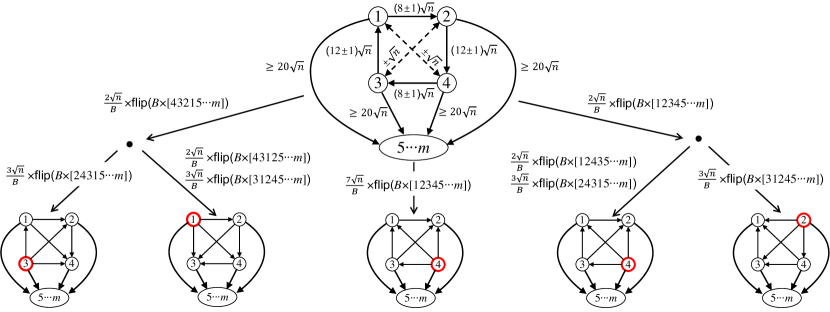
Figure 4: Violation template for C&P, general case.

Third, $\frac{n}{m!}\cdot\vec{1}$ is replaced by an arbitrary (but fixed) integer $\vec{u}=(u_{1},\ldots,u_{m!})$ via rounding, such that $|\vec{u}-\frac{n}{m!}\cdot\vec{1}|_{\infty}\leq 1$; $\left(\frac{n}{m!}\right)!$ is replaced by $\prod_{i=1}^{m!}(u_{i}!)$; and $\frac{n}{m!}+\alpha\sqrt{n}$ for any $\alpha$ appeared in the proof above is replaced by $\left\lceil\frac{n}{m!}\right\rceil+\alpha\sqrt{n}$. $\Box$

4 Other Semi-Random Impossibilities

The proof of Theorem 1 can leverage any proof diagram like Figure 1, that has the following three high-level features:

1. The diagram consists of constantly many nodes.

2. The diagram works all slightly perturbed root profiles.

3. $X$ is violated in each violation tree (scaled by $\sqrt{n}$) .

Therefore, any existing proof diagram for C&P, e.g., the one used in [9], can be used to prove Theorem 1. We chose the diagram in [43, Chapter 1] for its simplicity.

In this section, we prove semi-random impossibilities for the other three combinations of axioms, i.e., C&H, C&M, and C&S, by leveraging existing proof diagrams that have the three aforementioned features.

Theorem 2 (CC+half-way monotonicity)

For any fixed $m\geq 4$, any $\Pi$ that satisfies Assumption 1, any voting rule $r$, any $n\geq 24$, and any $1\leq B\leq\sqrt{n}$,

$$\widetilde{\text{\sc C\&H}}_{\Pi}^{\min}(r,n,B)=1-\Omega\left(\frac{B}{\sqrt{n}}\right)$$

Proof: The proof is similar to the proof of Theorem 1 and uses the same violation template (Figure 2). The main difference is that Claim 2 is replaced by the following claim.

Claim 6

For every $P\in\mathcal{P}_{n}$ and every $T\in\mathcal{T}_{P,B}$, CC or $\text{\sc HM}_{B}$ is violated in $T$.

The proof of this claim is straightforward: suppose there exists a pair of profiles $P_{1},P_{2}$ on a violation tree, such that $P_{2}$ is obtained from $P_{1}$ by flipping $B$ votes of $R$, where $r(P_{2})\succ_{R}r(P_{1})$, then $\text{\sc HM}_{B}$ fails at $P_{1}$. $\Box$

Theorem 3 (CC+Maskin monotonicity)

For any fixed $m\geq 3$, any $\Pi$ that satisfies Assumption 1, any voting rule $r$, any $n\in\mathbb{N}$, and any $1\leq B\leq\sqrt{n}$,

$$\widetilde{\text{\sc C\&M}}_{\Pi}^{\min}(r,n,B)=1-\Omega\left(\frac{B}{\sqrt{n}}\right)$$

Proof: The proof follows the same pattern as that of the proof of Theorem 1. For simplicity, we present the proof for the case where $m=3$, $\sqrt{n}$ is an integer, $B\mid\sqrt{n}$, and $m!\mid n$. The main difference is that we use a different proof diagram whose corresponding violation template is illustrated in Figure 5.

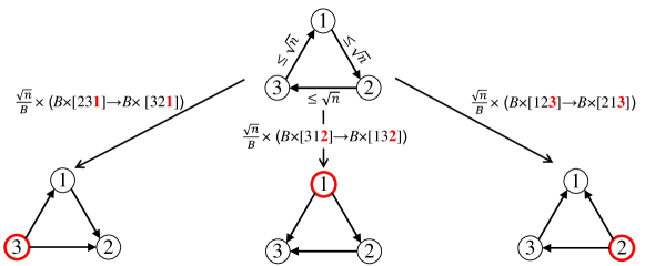
Figure 5: Violation template for C&M.

Formally, there are three branch starting from the root, each of which consists of $\frac{\sqrt{n}}{B}$ operations, and each operation consists of $B$ voters of the same vote $R_{1}$ changing to the same vote $R_{2}$ collaboratively:

• for the first branch $R_{1}=[231]$ and $R_{2}=[321]$;

• for the second branch $R_{1}=[312]$ and $R_{2}=[132]$;

• for the third branch $R_{1}=[123]$ and $R_{2}=[213]$.

Let $\mathcal{P}_{n}^{\text{\text{\sc C\&M}}}$ denote the set of $n$-profiles $P$, such that the weights on $1\rightarrow 2$, $2\rightarrow 3$, and $3\rightarrow 1$ in $P$’s WMG are between $0$ and $\sqrt{n}$. The violation template for C&M will be applied to profiles in $\mathcal{P}_{n}^{\text{\text{\sc C\&M}}}$, leading to violation trees for C&H, denoted by $\mathcal{T}_{n,B}^{\text{\sc C\&M}}$. We then prove the following claim.

Claim 7

For every $P\in\mathcal{P}_{n}^{\text{\sc C\&M}}$ and every $T\in\mathcal{T}_{P,B}^{\text{\sc C\&M}}$, CC or $\text{\sc MM}_{B}$ is violated in $T$.

To see why this claim holds, suppose $1$ is the winner of the root profile. We consider the left branch of the violation template in Figure 5. If the winner changes after any operation (which consists of $B$ votes of $[231]$ changing to $[321]$), then $\text{\sc MM}_{B}$ is violated. If $\text{\sc MM}_{B}$ is never violated on the left branch, then $1$ is the winner in the leaf node, which violates CC as $3$ is the Condorcet winner. The proof for $2$ (respective, $3$) being the winner is similar, by considering the middle (respectively, right) branch of Figure 5.

The rest of the proof, including the extension of the proof to the general case, is similar to the proof of Theorem 1. $\Box$

Theorem 4 (CC+strategy-proofness)

For any fixed $m\geq 3$, any $\Pi$ that satisfies Assumption 1, any voting rule $r$, any $n\in\mathbb{N}$, and any $1\leq B\leq\sqrt{n}$,

$$\widetilde{\text{\sc C\&S}}_{\Pi}^{\min}(r,n,B)=1-\Omega\left(\frac{B}{\sqrt{n}}\right)$$

Proof: When $m\geq 4$, Theorem 4 follows after Theorem 2, as SP is stronger than HM. The proof (for all $m\geq 3$) uses the same violation template in the proof of Theorem 3 (Figure 5). The main difference is to prove that each violation tree generated by the violation template contains a profile where CC or $\text{\sc SP}_{B}$ is violated, i.e., the following claim.

Claim 8

For every $P\in\mathcal{P}_{n}^{\text{\sc C\&M}}$ and every $T\in\mathcal{T}_{P,B}^{\text{\sc C\&M}}$, CC or $\text{\sc SP}_{B}$ is violated in $T$.

To see why the claim holds, notice that for any profile $P$ that is not a leaf in Figure 5, if the winner is different from the highlighted alternative, then $B$ voters have incentive to improve the winner at the previous profile. If $\text{\sc SP}_{B}$ is never violated at all profiles on the tree, then CC is violated at a leaf node. $\Box$

Recall that IC corresponds to $\Pi=\{{\pi}_{\text{uni}}\}$. Therefore, all semi-random impossibilities in this paper hold for IC.

Corrollary 1 (Quantitative Impossibilities under IC)

For any $X\in\{\text{\sc C\&P},\text{\sc C\&H},\text{\sc C\&M},\text{\sc C\&S}\}$, any $m\geq 4$ ($m\geq 3$ for C&M and C&S), any voting rule $r$, any sufficiently large $n\in\mathbb{N}$, and any $1\leq B\leq\sqrt{n}$,

$\hfill\Pr\nolimits_{P\sim\text{IC}}X(r,P,B)=1-\Omega\left(\frac{B}{\sqrt{n}}\right)\hfill$

Corollary 1 also implies that for any voting rule that satisfies CC, the likelihood for $r$ to satisfy Par, HM, MM, or SP, respectively, is $\Omega\left(\frac{B}{\sqrt{n}}\right)$ under IC.

5 Summary and Future Work

We prove the first set of semi-random impossibility results involving CC, showing that many existing voting rules are already optimal for C&P (for $B=1$) and C&S (for every $B\leq\sqrt{n}$). The proof technique has potential to strengthen other worst-case impossibilities to their semi-random variants. For future work, we conjecture that all bounds for the axioms are tight and can be achieved by many rules that satisfy CC. Other promising directions include addressing the limitations discussed in Section 1.2 and proving semi-random variants of other worst-case impossibility results, such as Arrow’s, Gibbard-Satterthwait (for non-CC rules), and various impossibility theorems in judgement aggregation. The proof technique developed in this paper (see Section 4) does not seem to be directly applicable, because existing proofs use diagrams that contains $\Theta(n)$ nodes.

References

- Arrow [1963] Kenneth Arrow. Social choice and individual values. New Haven: Cowles Foundation, 2nd edition, 1963. 1st edition 1951.
- Bai et al. [2022] Yushi Bai, Uriel Feige, Paul Gölz, and Ariel D. Procaccia. Fair Allocations for Smoothed Utilities. In Proceedings of ACM EC, 2022.
- Baumeister et al. [2020] Dorothea Baumeister, Tobias Hogrebe, and Jörg Rothe. Towards Reality: Smoothed Analysis in Computational Social Choice. In Proceedings of AAMAS, pages 1691–1695, 2020.
- Berry et al. [1995] Steven Berry, James Levinsohn, and Ariel Pakes. Automobile prices in market equilibrium. Econometrica, 63(4):841–890, 1995.
- Blum and Dunagan [2002] Avrim Blum and John D Dunagan. Smoothed Analysis of the Perceptron Algorithm for Linear Programming. In Proceedings of SODA, pages 905–914, 2002.
- Blum and Gölz [2021] Avrim Blum and Paul Gölz. Incentive-Compatible Kidney Exchange in a Slightly Semi-Random Model. In Proceedings of ACM EC, 2021.
- Blum and Spencer [1995] Avrim Blum and Joel Spencer. Coloring Random and Semi-Random k-Colorable Graphs. Journal of Algorithms, 19(2):204–234, 1995.
- Boodaghians et al. [2020] Shant Boodaghians, Joshua Brakensiek, Samuel B. Hopkins, and Aviad Rubinstein. Smoothed Complexity of 2-player Nash Equilibria. In Proceedings of FOCS, 2020.
- Brandt et al. [2017] Felix Brandt, Christian Geist, and Dominik Peters. Optimal bounds for the no-show paradox via SAT solving. Mathematical Social Sciences, 90:18–27, 2017.
- Brandt et al. [2021] Felix Brandt, Johannes Hofbauer, and Martin Strobel. Exploring the No-Show Paradox for Condorcet Extensions. In Mostapha Diss and Vincent Merlin, editors, Evaluating Voting Systems with Probability Models. Springer, 2021.
- Chung et al. [2008] Christine Chung, Katrina Ligett, Kirk Pruhs, and Aaron Roth. The Price of Stochastic Anarchy. In International Symposium on Algorithmic Game Theory, pages 303–314, 2008.
- Condorcet [1785] Marquis de Condorcet. Essai sur l’application de l’analyse à la probabilité des décisions rendues à la pluralité des voix. Paris: L’Imprimerie Royale, 1785.
- Diss and Merlin [2021] Mostapha Diss and Vincent Merlin, editors. Evaluating Voting Systems with Probability Models. Studies in Choice and Welfare. Springer International Publishing, 2021.
- Dobzinski and Procaccia [2008] Shahar Dobzinski and Ariel D. Procaccia. Frequent manipulability of elections: The case of two voters. In Proceedings of the Fourth Workshop on Internet and Network Economics (WINE), pages 653–664, Shanghai, China, 2008.
- Feige [2021] Uriel Feige. Introduction to Semi-Random Models. In Tim Roughgarden, editor, Beyond the Worst-Case Analysis of Algorithms. Cambridge University Press, 2021.
- Filmus et al. [2020] Yuval Filmus, Noam Lifshitz, Dor Minzer, and Elchanan Mossel. AND testing and robust judgement aggregation. In Proceedings of STOC, 2020.
- Fishburn [1974a] Peter C. Fishburn. Aspects of One-Stage Voting Rules. Management Science, 21(4):422–427, 1974a.
- Fishburn [1974b] Peter C. Fishburn. Simple voting systems and majority rule. Behavioral Science, 19(3):166–176, 1974b.
- Fishburn [1974c] Peter C. Fishburn. Paradoxes of voting. The American Political Science Review, 68(2):537–546, 1974c.
- Fishburn and Brams [1983] Peter C. Fishburn and Steven J. Brams. Paradoxes of Preferential Voting. Mathematics Magazine, 56(4):207–214, 1983.
- Friedgut et al. [2011] Ehud Friedgut, Gil Kalai, Nathan Keller, and Noam Nisan. A Quantitative Version of the Gibbard-Satterthwaite theorem for Three Alternatives. SIAM Journal on Computing, 40(3):934–952, 2011.
- Gehrlein and Fishburn [1978] William V. Gehrlein and Peter C. Fishburn. Coincidence probabilities for simple majority and positional voting rules. Social Science Research, 7(3):272–283, 1978.
- Gehrlein and Lepelley [2011] William V. Gehrlein and Dominique Lepelley. Voting Paradoxes and Group Coherence: The Condorcet Efficiency of Voting Rules. Springer, 2011.
- Gibbard [1973] Allan Gibbard. Manipulation of voting schemes: A general result. Econometrica, 41:587–601, 1973.
- Isaksson et al. [2010] Marcus Isaksson, Guy Kindler, and Elchanan Mossel. The Geometry of Manipulation: A Quantitative Proof of the Gibbard-Satterthwaite Theorem. In Proceedings of the 51st Annual Symposium on Foundations of Computer Science (FOCS), pages 319–328, Washington, DC, USA, 2010.
- Kalai [2002] Gil Kalai. A Fourier-theoretic perspective on the Condorcet paradox and Arrow’s theorem. Advances in Applied Mathematics, 29(3):412—426, 2002.
- Keller [2012] Nathan Keller. A tight quantitative version of Arrow’s impossibility theorem. Journal of the European Mathematical Society, 14:1331–1355, 2012.
- List and Pettit [2002] Christian List and Philip Pettit. Aggregating sets of judgments: An impossibility result. Economics and philosophy, 18(1):89–110, 2002.
- List and Pettit [2004] Christian List and Philip Pettit. Aggregating Sets of Judgments: Two Impossibility Results Compared. Synthese, 140:207–235, 2004.
- Liu and Xia [2022] Ao Liu and Lirong Xia. The Semi-Random Likelihood of Doctrinal Paradoxes. In Proceedings of AAAI, 2022.
- Maskin [1999] Eric Maskin. Nash Equilibrium and Welfare Optimality. Review of Economic Studies, 66:23—38, 1999.
- Mossel [2012] Elchanan Mossel. A quantitative Arrow theorem. Probability Theory and Related Fields, 154:49–88, 2012.
- Mossel and Racz [2015] Elchanan Mossel and Miklos Z. Racz. A quantitative Gibbard-Satterthwaite theorem without neutrality. Combinatorica, 35(3):317–387, 2015.
- Mossel et al. [2013] Elchanan Mossel, Krzysztof Oleszkiewicz, and Arnab Sen. On reverse hypercontractivity. Geometric and Functional Analysis, 23(3):1062–1097, 2013.
- Moulin [1983] Hervé Moulin. The Strategy of Social Choice. Elsevier, 1983.
- Moulin [1988] Hervé Moulin. Condorcet’s principle implies the no show paradox. Journal of Economic Theory, 45(1):53–64, 1988.
- Muller and Satterthwaite [1977] E. Muller and Mark Satterthwaite. The equivalence of strong positive association and strategy-proofness. Journal of Economic Theory, 14:412–418, 1977.
- Nehama [2013] Ilan Nehama. Approximately classic judgement aggregation. Annals of Mathematics and Artificial Intelligence, 68:91–134, 2013.
- Newenhizen [1992] Jill Van Newenhizen. The Borda Method Is Most Likely to Respect the Condorcet Principle. Economic Theory, 2(1):69–2–83, 1992.
- Paris [1975] David C. Paris. Plurality distortion and majority rule. Behavioral Science, 20(2):125–133, 1975.
- Pattanaik [1978] Prasanta K. Pattanaik. Strategy and group choice. Elsevier North-Holland, 1978.
- Peters [2017] Dominik Peters. Condorcet’s principle and the preference reversal paradox. In Proceedings of TARK, 2017.
- Peters [2019] Dominik Peters. Fair Division of the Commons. PhD thesis, Oxford University, 2019.
- Psomas et al. [2019] Alexandros Psomas, Ariel Schvartzman, and Matthew S. Weinberg. Smoothed Analysis of Multi-Item Auctions with Correlated Values. In Proceedings of ACM EC, 2019.
- Roughgarden [2021] Tim Roughgarden. Beyond the Worst-Case Analysis of Algorithms. Cambridge University Press, 2021.
- Saari [1995] Donald G. Saari. Basic Geometry of Voting. Springer, 1995.
- Sanver and Zwicker [2009] M. Remzi Sanver and William S. Zwicker. One-way monotonicity as a form of strategy-proofness. International Journal of Game Theory, 38:553–574, 2009.
- Satterthwaite [1975] Mark Satterthwaite. Strategy-proofness and Arrow’s conditions: Existence and correspondence theorems for voting procedures and social welfare functions. Journal of Economic Theory, 10:187–217, 1975.
- Spielman and Teng [2004] Daniel A. Spielman and Shang-Hua Teng. Smoothed analysis of algorithms: Why the simplex algorithm usually takes polynomial time. Journal of the ACM, 51(3), 2004.
- Spielman and Teng [2009] Daniel A. Spielman and Shang-Hua Teng. Smoothed Analysis: An Attempt to Explain the Behavior of Algorithms in Practice. Communications of the ACM, 52(10):76–84, 2009.
- Thurstone [1927] Louis Leon Thurstone. A law of comparative judgement. Psychological Review, 34(4):273–286, 1927.
- Train [2009] Kenneth E. Train. Discrete Choice Methods with Simulation. Cambridge University Press, 2nd edition, 2009.
- Xia [2020] Lirong Xia. The Smoothed Possibility of Social Choice. In Proceedings of NeurIPS, 2020.
- Xia [2021a] Lirong Xia. How Likely Are Large Elections Tied? In Proceedings of ACM EC, 2021a.
- Xia [2021b] Lirong Xia. The Semi-Random Satisfaction of Voting Axioms. In Proceedings of NeurIPS, 2021b.
- Xia [2022] Lirong Xia. How Likely A Coalition of Voters Can Influence A Large Election? arXiv:2202.06411, 2022.
- Xia and Conitzer [2008] Lirong Xia and Vincent Conitzer. A sufficient condition for voting rules to be frequently manipulable. In Proceedings of the ACM Conference on Electronic Commerce (EC), pages 99–108, Chicago, IL, USA, 2008.
- Xia and Zheng [2021] Lirong Xia and Weiqiang Zheng. The smoothed complexity of computing kemeny and slater rankings. In Proceedings of AAAI, 2021.