Analytic non-Abelian gravitating solitons in the Einstein-Yang-Mills-Higgs theory and transitions between them

Abstract

Two analytic examples of globally regular non-Abelian gravitating solitons in the Einstein-Yang-Mills-Higgs theory in (3+1)-dimensions are presented. In both cases, the space-time geometries are of the Nariai type and the Yang-Mills field is completely regular and of meron type (namely, proportional to a pure gauge). However, while in the first family (type I) $X_{0}=1/2$ (as in all the known examples of merons available so far) and the Higgs field is trivial, in the second family (type II) $X_{0}$ is not 1/2 and the Higgs field is non-trivial. We compare the entropies of type I and type II families determining when type II solitons are favored over type I solitons: the VEV of the Higgs field plays a crucial role in determining the phases of the system. The Klein-Gordon equation for test scalar fields coupled to the non-Abelian fields of the gravitating solitons can be written as the sum of a two-dimensional D’Alembert operator plus a Hamiltonian which has been proposed in the literature to describe the four-dimensional Quantum Hall Effect (QHE): the difference between type I and type II solutions manifests itself in a difference between the degeneracies of the corresponding energy levels.

1 Introduction

Non-Abelian solitons and instantons are fundamental pillars in our understanding of gauge theories beyond perturbation theories (see [1] [2] [3] [4] [5] and references therein). In many situations (such as in the cases of topological defects in the early universe), the effects of gravity cannot be neglected (see [6] and references therein). From a genuine General Relativistic viewpoint, non-Abelian gravitating solitons represent severe tests for well-known conjectures such as the no-hair conjecture. Consequently, it is a mandatory task to shed further light on these types of gravitating solitons. The gravitating solitons which have been analyzed in more details in the eighties and nineties are asymptotically flat and (almost always) numerical. However, it is worth noting that the requirement of asymptotic flatness is somewhat “foreign” to the requirement of regularity in the sense that while gravitating solitons must be regular by definition, genuine non-Abelian and globally regular gravitating solitons need not to be asymptotically flat. The first example was discovered by Bartnik and McKinnon (BK) [7]. Soon after the BK gravitating solitons, genuine non-Abelian black holes were also constructed numerically in [8] [9] [10]. These results closely related to the no-hair conjecture and to the black holes uniqueness theorem attracted a lot of attention since then (see, for instance, [11] [12] [13] [14] [15] [16] [17] and references therein). In the present paper, we will be mainly interested in the construction of analytic non-Abelian gravitating solitons. To the best of our knowledge, the only known analytic example in (3+1) dimensions of a globally regular gravitating soliton with “bona fide” non-Abelian gauge field has been found in [18] (many nice numerical examples are described in [11] [12] [13] [14] [15] [16] [17] and references therein). Such remarkable analytic solution has been found in the Einstein-Yang-Mills-dilaton system: so far it has not been possible to extend this solution to Einstein-Yang-Mills theory without dilatonic coupling. The main goal of the present manuscript is to construct two types of globally regular analytic non-Abelian gravitating solitons in the Einstein-Yang-Mills-Higgs system in (3+1)-dimensions without any dilatonic coupling and to analyze the transitions between these families as well as their remarkable physical properties.

An obvious question is: why should one insist so much on finding analytic solutions if these equations can be solved numerically? Since the pioneering works of Bartnik and McKinnon mentioned above, very powerful numerical techniques have been proposed in the literature to construct non-Abelian gravitating solitons (see, for instance, [11], [19] [20] [21] and references therein). There are really good reasons to strive for analytic solutions nevertheless.

Besides the obvious fact that a systematic tool to construct analytic gravitating solitons can greatly enlarge our understanding of these configurations, the main reason is that the availability of analytic gravitating non-Abelian solitons allows to disclose phenomena that would be very difficult to see otherwise. In particular, the present formalism discloses the possibility to have transitions between these solitons and a very surprising analogy with the four-dimensional Quantum Hall Effect (QHE) which will be discussed in a moment.

As we are seeking for genuine non-Abelian effects, meron types configurations (introduced in [22]) are really good candidates as such configurations can only appear in non-Abelian gauge theories (see [2] and references therein). A gauge potential of meron type can be defined as proportional to a pure gauge: $A_{\mu}=X_{0}U^{-1}\partial_{\mu}U$ (with $X_{0}\neq 0,1$): such a gauge potential is non-trivial due to the presence of the commutator in the non-Abelian field-strength. On the other hand, in Abelian gauge theories, a gauge potential which is proportional to a pure gauge is itself a pure gauge and therefore is trivial. Consequently, merons are bona fide non-Abelian configurations. Since the pioneering works [23] [24], the important role of these types of configurations in understanding the non-perturbative phase of QCD has been widely recognized (see [25] and references therein).

All the known examples of merons so far have $X_{0}=1/2$; thus, a first question that we will answer (affirmatively) is: is it possible to have non-trivial merons configurations with $X_{0}\neq 1/2$ ?

The second and most difficult issue related to merons is the following. Merons on flat spaces are necessarily singular: they play an important role (see [23] [24] [25] and references therein) as “elementary components” of instantons (since an instanton can be thought as a bound state of two merons). However, on flat spaces, merons cannot be observed directly (as they have infinite Euclidean action/energy). When Yang-Mills theory is coupled with General Relativity (GR), it has been possible to construct analytic examples of merons-black holes [26] [27] [28] [29]. Thus, in a sense, meron-black holes can be observed directly (some peculiar effects have been discussed in [29]), but the meron singularity is still there (although hidden behind the horizon). Consequently, the examples in [26] [27] [28] [29] are not gravitating solitons but rather non-Abelian black holes. The very important question is: can we construct analytic examples of gravitating merons in which the typical singularity of the merons disappears completely? In the following, we will show that it is indeed possible to construct globally regular gravitating merons solutions free of any singularity. Moreover, there are two different families of regular gravitating merons that compete against each other leading to quite interesting phenomena.

A further by-product of the present analysis appears when one analyzes the dynamics of a test field charged under the gauge group moving on these gravitating non-Abelian solitons. The effective Hamiltonian determining the dynamics of charged test fields includes the Hamiltonian describing the four-dimensional Quantum Hall Effect (4DQHE) introduced in [30] and further analyzed in [31] [32] [33] [34] [35] [36] [37] and references therein. Such deep generalization of the usual theory of the two-dimensional QHE has also been confirmed in condensed matter experiments (see [38] [39] and references therein). However, until now, there have been very few concrete realizations of the 4DQHE in high energy physics using fields arising in the standard model of particles physics minimally coupled to GR. In this work, we fill the gap by providing a setting (in the Einstein-Yang-Mills-Higgs theory) in which an explicit realization of the physical features of the 4DQHE is possible. A very intriguing effect is that the two families of non-Abelian gravitating solitons can be distinguished by looking at the degeneracies of the corresponding energy levels.

The paper is organized as follows: In Section II, we present the model and give our ansatz and the corresponding field equations. In Sections III and IV, we construct the two families of the analytic regular solutions of the Einstein-Yang-Mills-Higgs theory in (3+1)-dimensions. In Section V, we introduce a standard coordinate system of the Nariai class of spacetime to work out the surface gravity and the temperature of the system. In Section VI, we present the entropy functions of the two types of the solutions and provide some useful plots of the entropy functions to see which configuration is favored for given sets of the physical parameters. In Section VII, we analyze the Klein-Gordon equation to disclose the difference between two types of solutions by making use of the four-dimensional quantum hall effects. In the last Section, our conclusions are drawn.

2 Action and ansatz

The starting point is the action of the (3+1)-dimensional Einstein-Yang-Mills-Higgs field:

$$I=\int d^{4}x\sqrt{-g}\Big{(}\frac{R-2\Lambda}{\kappa}+\frac{1}{4e^{2}}\text{Tr}\big{[}F_{\mu\nu}F^{\mu\nu}\big{]}+\frac{1}{2e^{2}}\text{Tr}\big{[}D_{\mu}\Phi^{\ast}D^{\mu}\Phi\big{]}-2V(\Phi^{\ast}\Phi)\Big{)}\ ,$$

where $R$, $\Lambda$, and $V(\Phi^{\ast}\Phi)$ are the Ricci scalar of the space-time, the cosmological constant, and the self-interacting Higgs potential, respectively. The dimensionless constant $e$ is the gauge coupling and $\kappa=8\pi G$ for the gravitational constant $G$. The field strength of the Yang-Mills field $A_{\mu}$ is $F_{\mu\nu}=\partial_{\mu}A_{\nu}-\partial_{\nu}A_{\mu}+[A_{\mu},A_{\nu}]$ and the gauge-covariant derivative is $D_{\mu}=\nabla_{\mu}+[A_{\mu},\cdot\ ]$. In this notation, the Einstein’s equations are written as

$$R_{\mu\nu}-\frac{1}{2}g_{\mu\nu}R+\Lambda g_{\mu\nu}=\kappa T_{\mu\nu}\ ,$$

where the energy-momentum tensor is given by

$$T_{\mu\nu}=T_{\mu\nu}^{\text{(YM)}}+T_{\mu\nu}^{\text{(H)}}\ ,$$

where

$$T_{\mu\nu}^{\text{(YM)}} =-\frac{1}{2e^{2}}\text{Tr}\Big{(}g^{\alpha\beta}F_{\mu\alpha}F_{\nu\beta}-\frac{1}{4}g_{\mu\nu}F^{\alpha\beta}F_{\alpha\beta}\Big{)}\ ,$$ (1)

$$T_{\mu\nu}^{\text{(H)}} =-\frac{1}{2e^{2}}\text{Tr}\Big{(}D_{\mu}\Phi D_{\nu}\Phi-\frac{1}{2}g_{\mu\nu}D^{\alpha}\Phi D_{\alpha}\Phi\Big{)}-g_{\mu\nu}V(\Phi^{\ast}\Phi)\ .$$ (2)

The equations for the Higgs and Yang-Mills fields are

$$g^{\mu\nu}D_{\mu}D_{\nu}\Phi =-e^{2}\frac{dV}{d(\Phi^{\ast}\Phi)}\Phi\ ,$$ (3)

$$D^{\mu}F_{\mu\nu} =[\Phi,D_{\nu}\Phi]\ .$$ (4)

The Higgs potential is given by

$$V(\Phi^{\ast}\Phi)=\lambda(\Phi^{\ast}\Phi-v_{0}^{2})^{2}\ ,$$

where $\lambda$ is the self-interacting coupling constant of the Higgs fields. We consider this Einstein-Yang-Mills-Higgs (briefly, EYMH) system in the space-time with the metric given by

$$ds^{2}=F_{0}\big{[}-2y(u,v)dudv+L^{2}\big{(}d\theta^{2}+\sin^{2}\theta\ d\phi^{2}\big{)}\big{]}\ ,$$

where $L$ and $F_{0}$ are constant (without loss of generality $F_{0}$ can be assumed to be positive). As has been already emphasized, the Yang-Mills field is assumed to have the meron form

$$A_{\mu}=X_{0}\ U^{-1}\partial_{\mu}U\ ,$$ (5)

where $X_{0}$ is a constant such that $X_{0}\neq 0,1$. The $SU(2)$-valued scalar field $U$ is parametrized as

$$U^{\pm 1}(x^{\mu})=\pm Y^{A}(x^{\mu})t_{A}\ ;\qquad Y^{1}=\sin\theta\cos\phi\ ,\,Y^{2}=\sin\theta\sin\phi\ ,\,Y^{3}=\cos\theta\ ,$$

where $t_{A}=i\sigma_{A}$ for the Pauli matrix $\sigma_{A}$ The Higgs field is given in an adjoint representation by

$$\Phi=W_{0}\ U\ ,$$

where the constant $W_{0}$ has to be determined solving the Higgs field equations which (with the ansatz defined above) reduce to the single algebraic equation

$$2\lambda e^{2}F_{0}L^{2}(W_{0}^{2}-v_{0}^{2})+(2X_{0}-1)^{2}=0\ .$$ (6)

The Yang-Mills equations (4) also reduce to the following single algebraic equation;

$$(2X_{0}-1)\big{[}L^{2}F_{0}W_{0}^{2}-X_{0}(1-X_{0})\big{]}=0\ .$$ (7)

From Eqs. (6) and (7) it is clear that there are two families of solutions.

The first family (which will be called type I) corresponds to the usual meron solution together with the condition that the Higgs field profile $W_{0}$ is in the “VEV”:

$$X_{0}=\frac{1}{2}\ ,\ W_{0}^{2}=v_{0}^{2}\ .$$ (8)

The second family (which will be called type II) corresponds to the conditions

$$X_{0}\neq\frac{1}{2}\ ,\ W_{0}^{2}\neq v_{0}^{2}\ .$$ (9)

The explicit form of the type II solution will be discussed in the next sections.

The nonvanishing components of the Einstein’s equation are found to be

$$e^{2}\big{[}\kappa\lambda(W_{0}^{2}-v_{0}^{2})^{2}+\Lambda\big{]}(F_{0}L^{2})^{2}+\big{[}\kappa W_{0}^{2}(2X_{0}-1)^{2}-e^{2}\big{]}(F_{0}L^{2})+2\kappa X_{0}^{2}(1-X_{0})^{2}=0\ ,$$ (10)

$$\frac{1}{y}\partial_{u}\partial_{v}y-\frac{1}{y^{2}}\partial_{u}y\cdot\partial_{v}y+\Big{(}\frac{2\kappa X_{0}^{2}(1-X_{0})^{2}}{e^{2}(F_{0}L^{2})^{2}}-\kappa\lambda(W_{0}^{2}-v_{0}^{2})^{2}-\Lambda\Big{)}F_{0}y=0\ .$$ (11)

3 Type I family: standard Meronic configuration

It follows from Eq. (6) that the value of $W_{0}$ is precisely the vacuum expectation value $v_{0}$ if and only if the configuration of the gauge field is a meron:

$$W_{0}=v_{0}\qquad\Longleftrightarrow\qquad X_{0}=\frac{1}{2}\ .$$

In this case, the Eqs. (6) and (7) are automatically satisfied and the Eq. (10) fixes the value of $F_{0}L^{2}$, which is the size of the $S^{2}$, in terms of the cosmological constant $\Lambda$ and of the other parameters:

$$\Lambda(F_{0}L^{2})^{2}-F_{0}L^{2}+\frac{\kappa}{8e^{2}}=0\ .$$

This equation admits one or two positive roots for $F_{0}L^{2}$ and the number of roots depends on the range of physical parameters as follows:

$$\begin{cases}F_{0}L^{2}=\frac{1\pm\sqrt{1-\kappa\Lambda/2e^{2}}}{2\Lambda}>0\qquad\text{when}\quad 0<\Lambda<2e^{2}/\kappa\ ,\\ F_{0}L^{2}=\frac{1-\sqrt{1-\kappa\Lambda/2e^{2}}}{2\Lambda}>0\qquad\text{when}\quad\Lambda<0\ ,\\ F_{0}L^{2}=\frac{1}{2\Lambda}\qquad\text{when}\quad\Lambda=2e^{2}/\kappa\ ,\\ F_{0}L^{2}=\frac{\kappa}{8e^{2}}\qquad\text{when}\quad\Lambda=0\ .\end{cases}$$ (12)

4 Analytic Solutions of type II

The Higgs equation (6) has the solution

$$X_{0}=\frac{1}{2}\Big{(}1\pm\sqrt{2\lambda e^{2}F_{0}L^{2}(v_{0}^{2}-W_{0}^{2})}\Big{)}\ ,$$ (13)

only when the constant $W_{0}$ lies in the range of

$$W_{0}^{2}\leq v_{0}^{2}\ .$$ (14)

When $W_{0}=v_{0}$ the configuration of the Yang-Mills field becomes that of a standard meron $X_{0}=1/2$ (and the Higgs field becomes trivial as it completely disappears from the energy-momentum tensor) so the solutions become of type I. In this section, we will discuss $W_{0}$ such that $W_{0}^{2}<v_{0}^{2}$ (the type I solutions will be discussed in the next section). The Yang-Mills equation (7) gives

$$F_{0}L^{2}=\frac{1}{2\big{(}\lambda e^{2}(v_{0}^{2}-W_{0}^{2})+2W_{0}^{2}\big{)}}\ .$$ (15)

Using (13) and (15) in Eq. (10), we obtain a quadratic equation for $W_{0}^{2}$

$$\kappa(2-\lambda e^{2})(W_{0}^{2})^{2}-2e^{2}(2-\lambda e^{2})W_{0}^{2}+e^{2}\big{[}\lambda v_{0}^{2}(\kappa v_{0}^{2}-2e^{2})+\Lambda\big{]}=0\ .$$ (16)

This equation admits one or two positive roots for $W_{0}^{2}$ within $\big{(}0,v_{0}^{2}\big{)}$. Let us examine the corresponding configurations of the physical system in order.

4.1 Type II configurations

There are three cases that must be considered separately.

Option 1) Eq. (16) can have two positive roots for $W_{0}^{2}$ (in this case type II configurations can be divided into two sub-families, one for each positive root of Eq. (16)).

Option 2) Eq. (16) can have one positive roots for $W_{0}^{2}$ (in this case, there is just one family of type II configurations).

Option 3) Eq. (16) has no positive roots for $W_{0}^{2}$ (in this case, there is no family of type II configurations).

Whether (for instance) option 1 is realized instead of options 2 or 3 depends on the values of the parameters of the models. Especially relevant are the Higgs coupling constant $\lambda$ and the VEV $v_{0}^{2}$. Option 1 is the most interesting one from the thermodynamical viewpoint since, in this case, there is a competition between three types of solutions: the standard meron $X_{0}=1/2$ and $W_{0}^{2}=v_{0}^{2}$ (type I), the type II solution corresponding to the larger positive root of Eq. (16) and the type II solution corresponding to the smaller positive root of Eq. (16). As it will be discussed in the next sections, this opens the very intriguing possibility of multiple transitions between these three types of solutions. Option 2 is the second most interesting case since there is a competition between two types of solutions: the standard meron $X_{0}=1/2$ and $W_{0}^{2}=v_{0}^{2}$ (type I), and the only viable type II solution corresponding to the unique positive root of Eq. (16). On the other hand, when option 3 is realized, no transition is possible since the only viable non-Abelian gravitating solitons belong to type I. In the discussion below, it will be convenient to introduce the following boundary values of $\Lambda$:

$$\Lambda_{1}=\lambda v_{0}^{2}(2e^{2}-\kappa v_{0}^{2})\ ,\qquad\Lambda_{2}=\frac{2v_{0}^{2}(2e^{2}-\kappa v_{0}^{2})}{e^{2}}\ ,\qquad\Lambda_{3}=\Lambda_{1}+\frac{e^{2}(2-\lambda e^{2})}{\kappa}\ ,$$

4.1.1 Option 1: $W_{0}^{2}$ has two positive roots within $\big{(}0,v_{0}^{2}\big{)}$

The Eq. (16) has two different positive roots

$$\big{(}W_{0}^{(\pm)}\big{)}^{2}=\frac{e^{2}}{\kappa}\big{(}1\pm\sqrt{D_{1}}\big{)}\ ,$$ (17)

where

$$D_{1}=1+\frac{\kappa\big{[}\lambda v_{0}^{2}(\kappa v_{0}^{2}-2e^{2})+\Lambda\big{]}}{e^{2}(\lambda e^{2}-2)}\ .$$ (18)

when one of the following sets of conditions is satisfied:

1. When $0<\lambda<2/e^{2}$:

   $$e^{2}/v_{0}^{2}<\kappa<2e^{2}/v_{0}^{2}\quad\text{and}\quad\Lambda_{2}<\Lambda<\Lambda_{3}\ ,$$ (19)

   $$\kappa\geq 2e^{2}/v_{0}^{2}\quad\text{and}\quad\Lambda_{1}<\Lambda<\Lambda_{3}\ .$$ (20)

2. When $2/e^{2}<\lambda$:

   $$e^{2}/v_{0}^{2}<\kappa<2e^{2}/v_{0}^{2}\quad\text{and}\quad\Lambda_{3}<\Lambda<\Lambda_{2}\ ,$$ (21)

   $$\kappa\geq 2e^{2}/v_{0}^{2}\quad\text{and}\quad\Lambda_{3}<\Lambda<\Lambda_{1}\quad\ .$$ (22)

4.1.2 Option 2: $W_{0}^{2}$ has one positive root in $\big{(}0,v_{0}^{2}\big{)}$

The equation (16) has one positive root $W_{0}^{2}\in\big{(}0,v_{0}^{2}\big{)}$ and one negative root $W_{0}^{2}\in\big{(}-\infty,0\big{)}$ when the conditions given below are satisfied:

1. When $0<\lambda<\Lambda/v_{0}^{2}(2e^{2}-\kappa v_{0}^{2})$:

   $$0<\kappa<2e^{2}/v_{0}^{2}\quad\text{and}\quad 0<\Lambda<\Lambda_{2}\ ,$$ (23)

   $$\kappa>2e^{2}/v_{0}^{2}\quad\text{and}\quad\Lambda_{2}<\Lambda<0\ .$$ (24)

2. When $\lambda>\Lambda/v_{0}^{2}(2e^{2}-\kappa v_{0}^{2})$:

   $$0<\kappa<2e^{2}/v_{0}^{2}\quad\text{and}\quad\Lambda_{2}<\Lambda\ ,$$ (25)

   $$\kappa>2e^{2}/v_{0}^{2}\quad\text{and}\quad\Lambda<\Lambda_{2}\ .$$ (26)

In this case, the physical solution is $W_{0}=W_{0}^{(+)}$ given in Eq. (17).

When $W_{0}^{2}$ has a positive double root in $\big{(}0,v_{0}^{2}\big{)}$

The Eq. (16) has a positive double root

$$\big{(}W_{0}^{(D)}\big{)}^{2}=\frac{\kappa\lambda v_{0}^{2}(1+2e^{2})-(4-\lambda)e^{2}}{2\kappa\big{[}\lambda(1+e^{2})-2\big{]}}\ ,$$

when the following condition is satisfied:

$$\lambda\neq\frac{2}{e^{2}}\quad\text{and}\quad\kappa>\frac{e^{2}}{v_{0}^{2}}$$ (27)

In this case, the cosmological constant $\Lambda$ and the other coupling constants are related by

$$\lambda(\kappa v_{0}^{2})^{2}-2\lambda e^{2}(\kappa v_{0}^{2})+e^{2}(2-\lambda e^{2})+\kappa\Lambda=0\ .$$

4.1.3 Option 3: $W_{0}^{2}$ has no positive roots within $\big{(}0,v_{0}^{2}\big{)}$

The Eq. (16) has no positive root within $\big{(}0,v_{0}^{2}\big{)}$ when one of the following sets of the conditions is satisfied:

1. When $0<\lambda<2/e^{2}$:

   $$0<\kappa\leq 2e^{2}/v_{0}^{2}\quad\text{and}\quad\Lambda\leq\Lambda_{1}\ ,$$ (28)

   $$\kappa>2e^{2}/v_{0}^{2}\quad\text{and}\quad\Lambda\leq\Lambda_{2}\ .$$ (29)

2. When $\lambda>2/e^{2}$:

   $$0<\kappa\leq 2e^{2}/v_{0}^{2}\quad\text{and}\quad\Lambda\geq\Lambda_{1}\ ,$$ (30)

   $$\kappa>2e^{2}/v_{0}^{2}\quad\text{and}\quad\Lambda\geq\Lambda_{2}\ .$$ (31)

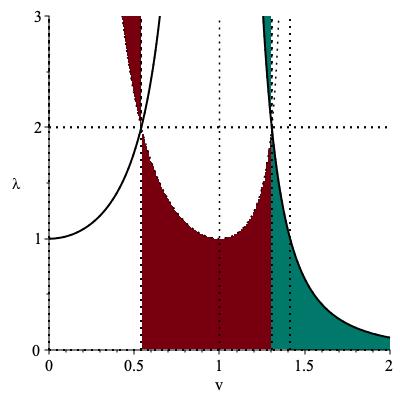
(a) $e=1$, $\Lambda=1$, $\kappa=1$

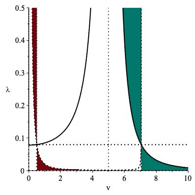
(b) $e=5$, $\Lambda=1$, $\kappa=1$

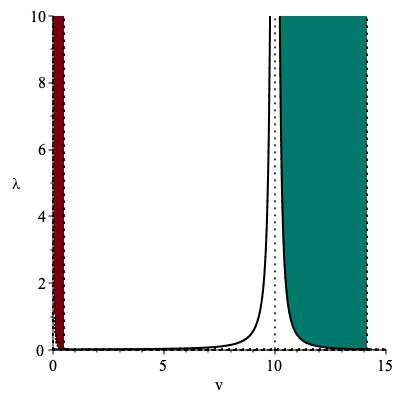
(c) $e=10$, $\Lambda=1$, $\kappa=1$

Figure 1: The burgundy, green, and white regions show the range of couplings on which Eq. (16) has one, two, and no positive root of $W_{0}^{2}$ in $(0,v_{0}^{2})$, respectively. The solid lines represent the configurations with double roots.

4.2 Equation for $y(u,v)$ and Ricci Scalar (both type I and II)

In all of the above cases, the only non-trivial differential equation is the $\theta\theta$-component of the Einstein’s equations, which can be written as

$$\frac{1}{y^{2}}\partial_{u}\partial_{v}y-\frac{1}{y^{3}}\partial_{u}y\cdot\partial_{v}y+\frac{1}{y_{0}}=0\ ,$$ (32)

where

$$y_{0}=\Big{[}\frac{2\kappa}{L^{4}e^{2}F_{0}}X_{0}^{2}(1-X_{0})^{2}-\kappa\lambda F_{0}(W_{0}^{2}-v_{0}^{2})^{2}-\Lambda F_{0}\Big{]}^{-1}\ .$$ (33)

The solution to this equation is found to be

$$y(u,v)=-2C_{2}C_{3}y_{0}\operatorname{sech}^{2}(C_{1}+C_{2}u+C_{3}v)\ .$$ (34)

Correspondingly, the Ricci scalar $R_{s}$ is given by

$$R_{s}=\frac{2}{F_{0}}\Big{(}\frac{2}{y_{0}}+\frac{1}{L^{2}}\Big{)}\ .$$ (35)

The gauge field for both type I and type II are regular and free of singularity, since the following scalars invariant under coordinate transformation are found to be

$$\text{Tr}\big{(}F_{\mu\nu}F^{\mu\nu}\big{)}=-\frac{16X_{0}^{2}(1-X_{0})^{2}}{F_{0}^{2}L^{4}}\ ,\qquad\text{Tr}\big{(}A_{\mu}A^{\mu}\big{)}=-\frac{4X_{0}^{2}}{F_{0}L^{2}}\ .$$

One can also find that the space-time of this solution belongs to the Petrov type D.

5 Thermodynamics in Nariai Coordinates

Without loss of generality, one can rescale the coordinates $u$ and $v$ to choose the constants $C_{1}=0$, $C_{2}=1$, and $C_{3}=-1$. Then, the metric becomes

$$ds^{2}=-2F_{0}y_{0}\operatorname{sech}^{2}(u-v)dudv+F_{0}L^{2}d\Omega_{2}^{2}\ .$$ (36)

Introducing new coordinates $\tilde{t}$ and $R$ given by

$$u=\frac{\tilde{t}+R}{2}\ ,\qquad v=\frac{\tilde{t}-R}{2}\ ,$$

we can express the metric (36) becomes

$$ds^{2}=\frac{F_{0}y_{0}}{2}\operatorname{sech}^{2}(R)\big{(}-d\tilde{t}^{2}+dR^{2}\big{)}+F_{0}L^{2}d\Omega_{2}^{2}\ .$$ (37)

Again, introducing new coordinates $t$ and $r$ given by

$$t=r_{0}\tilde{t}\ ,\qquad\operatorname{sech}^{2}(R)\equiv 1-\frac{r^{2}}{r_{0}^{2}}\$$

the metric (37) can be transformed to the following metric representing a product space $dS_{2}\times S^{2}$:

$$ds^{2}=\frac{F_{0}y_{0}}{2r_{0}^{2}}\Big{[}-\Big{(}1-\frac{r^{2}}{r_{0}^{2}}\Big{)}dt^{2}+\frac{1}{1-\frac{r^{2}}{r_{0}^{2}}}dr^{2}\Big{]}+F_{0}L^{2}d\Omega_{2}^{2}\ .$$ (38)

This metric clearly shows that our space-time belongs to the Nariai family of space-times. With this coordinate system, it is straightforward to compute the surface gravity $\kappa$

$$\kappa=\frac{1}{r_{0}}\ ,$$

so that the temperature $T$ is found to be

$$T=\frac{1}{2\pi r_{0}}\ .$$

It should be noticed that (as it will be shown in the next section) the entropies of the two different families are inversely proportional to $r_{0}^{2}$, so that the ratio of the entropies (which determines which family prevails) is independent of $r_{0}^{2}$. In the next section, we will compute the entropy functions of type I and type II and find the range of the physical parameters where one of these type dominates the other.

6 Thermodynamics and Transitions between families

One of the most interesting outcomes of the present analysis is that there are different types of gravitating non-Abelian solitons in the Einstein-Yang-Mills-Higgs in the sector described above. The space-time geometry is of Nariai type, while the Yang-Mills field can be either a standard ($X_{0}=1/2$) meron with a trivial Higgs field or a non-standard meron with a non-trivial Higgs field. Hence, the natural question is: which one of the gravitating solitons described above will prevail? The analysis shows that the answer to this question depends in a crucial way both on the Higgs coupling and on the “VEV” of the Higgs field itself. There are two related tools to answer this question: the first is the computation of the “entropy” of the solutions, the second is the computation of the Euclidean action of the different configurations (as it will be shown, these tools give consistent answers).

6.1 Entropy function

The entropy function(al) of space-times of the form $AdS_{2}\times S^{D-2}$ (associated to the near-horizon geometries of extremal black holes) for an arbitrary dimension $D$ was studied by A. Sen [40]. The entropy function of this class of space-times is the product of $2\pi$ with the Legendre transform of the Lagrangian density integrated over $S^{D-2}$. Since the electric fields associated with the gauge fields play the role of configuration variables, this entropy is a Routhian density over $AdS_{2}$ rather than a Hamiltonian density. A direct application of the Sen’s method to Nariai class shows that the entropy of a Nariai space-time is “minus” Routhian density over $dS_{2}$ [41]. The first step corresponds to the on-shell evaluation of the Lagrangian of the matter field (while the second step corresponds to integrate the on-shell Lagrangian for the matter field over $S^{2}$). The on-shell Lagrangian reads

$$\frac{1}{4e^{2}}\text{Tr}\big{[}F_{\mu\nu}F^{\mu\nu}\big{]} =-\frac{1}{4e^{2}}\Big{(}\frac{4X_{0}(1-X_{0})}{F_{0}L^{2}}\Big{)}^{2}\ ,$$

$$\frac{1}{2e^{2}}\text{Tr}\big{[}D_{\mu}\Phi^{\ast}D^{\mu}\Phi\big{]} =-\frac{1}{2e^{2}}\Big{(}\frac{2W_{0}(2X_{0}-1)}{F_{0}L^{2}}\Big{)}^{2}\ ,$$ (39)

and the Ricci scalar was given by (35). In the Nariai coordinates, we have

$$\sqrt{-g}=\frac{F_{0}^{2}y_{0}L^{2}}{2r_{0}^{2}}\sin\theta\ .$$

Since the system has no electric field, the Routhian density $H$ becomes

$$H = -\oint_{S^{2}}d\theta d\phi\sqrt{-g}\,\mathcal{L}$$ (40)

$$= -\frac{2\pi F_{0}^{2}y_{0}L^{2}}{r_{0}^{2}}\Big{[}\frac{2}{F_{0}}\Big{(}\frac{2}{y_{0}}+\frac{1}{L^{2}}\Big{)}-\frac{1}{4e^{2}}\Big{(}\frac{4X_{0}(1-X_{0})}{F_{0}L^{2}}\Big{)}^{2}-\frac{1}{2e^{2}}\Big{(}\frac{2W_{0}(2X_{0}-1)}{F_{0}L^{2}}\Big{)}^{2}-\lambda(W_{0}^{2}-v_{0}^{2})^{2}\Big{]}\ ,$$

where $\mathcal{L}$ is the Lagrangian of the system. The computations given in [40, 41] tells us that the entropy function S will be given by

$$S=-2\pi H_{\text{max}}\ .$$ (41)

where $H_{\text{max}}$ is the maximum value with respect to $F_{0}y_{0}$ and $F_{0}L^{2}$ (note that $H_{\text{max}}$ is negative so that the entropy is positive definite as it should). The entropy function of the system is found to be

$$S=\begin{cases}\dfrac{4\pi^{2}}{\kappa e^{2}r_{0}^{2}\big{(}\kappa\lambda(W_{0}^{2}-v_{0}^{2})^{2}+\Lambda\big{)}}\Big{(}e^{2}-\kappa W_{0}^{2}(2X_{0}-1)^{2}+\sqrt{Q}\Big{)}&\text{for}\ W_{0}^{2}\neq v_{0}^{2}\vspace{0.2in}\\ \dfrac{4\pi^{2}\big{(}1+\sqrt{1-\kappa\Lambda/2e^{2}}\big{)}}{\kappa\Lambda r_{0}^{2}}&\text{for}\ W_{0}^{2}=v_{0}^{2}\ .\end{cases}$$

where

$$Q=\big{(}e^{2}-\kappa W_{0}^{2}(2X_{0}-1)^{2}\big{)}^{2}-8\kappa e^{2}X_{0}^{2}(1-X_{0})^{2}\big{(}\kappa\lambda(W_{0}^{2}-v_{0}^{2})^{2}+\Lambda\big{)}\ .$$

6.2 Euclidean action

In order to compute the Euclidean action for both families, it is convenient to define the ”sizes” of the $dS_{2}$ and $S^{2}$ as

$$v_{1}=F_{0}y_{0}\ ,\qquad v_{2}=F_{0}L^{2}\ ,$$

respectively. Then, the Euclidean action can be written as

$$I_{E}=\frac{4\pi^{2}v_{1}v_{2}}{r_{0}^{2}}\Big{[}2\Big{(}\frac{1}{v_{1}}+\frac{1}{v_{2}}\Big{)}-\frac{1}{4e^{2}}\Big{(}\frac{4X_{0}(1-X_{0})}{v_{2}}\Big{)}^{2}-\frac{1}{2e^{2}}\Big{(}\frac{2W_{0}(2X_{0}-1)}{v_{2}}\Big{)}^{2}-\lambda(W_{0}^{2}-v_{0}^{2})^{2}\Big{]}\ .$$

The on-shell conditions that extremize the Euclidean action are found to be

$$2\lambda e^{2}(W_{0}^{2}-v_{0}^{2})v_{2}+(2X_{0}-1)^{2} =0\ ,$$ (42)

$$(2X_{0}-1)\big{[}W_{0}^{2}v_{2}-X_{0}(1-X_{0})\big{]} =0\ ,$$ (43)

$$e^{2}\big{[}\kappa\lambda(v_{0}^{2}-W_{0}^{2})^{2}+\Lambda\big{]}v_{2}^{2}+\big{[}\kappa(2X_{0}-1)^{2}W_{0}^{2}-e^{2}\big{]}v_{2}+2\kappa X_{0}^{2}(1-X_{0})^{2} =0\ ,$$ (44)

$$\big{[}e^{2}\big{(}\kappa\lambda(v_{0}^{2}-W_{0}^{2})^{2}+\Lambda\big{)}v_{2}^{2}-2\kappa X_{0}^{2}(1-X_{0})^{2}\big{]}v_{1}+e^{2}v_{2} =0\$$ (45)

One can easily check that these equations are equivalent to the equations of motion (6), (7), (10), and (33). Thus, it follows from (41) that the on-shell Euclidean action is precisely equal to the entropy of the system. The overall factor $2\pi$ should be understood as the circumference of the imaginary time.

6.3 Useful Plots

The previous analysis showed that a critical parameter to determine which of the solutions is thermodynamically favored is the VEV of the Higgs field $v_{0}^{2}$. Here below, we will include the plots which clarify the comparisons between the two families of gravitating solitons in the three options defined in the previous sections (depending on the number of roots in the equation for $W_{0}^{2}$).

6.3.1 Option 1 Plots

In the “Option 1 case” defined in the previous sections, Eq. (16) has two different positive real roots (let us call them $\left(W_{0}^{2}\right)^{\pm}$ where the $+$ stands for the larger root and the $-$ for the smaller one). In this case, multiple transitions may appear as the thermodynamics is determined by the comparison of three solutions: the type I, the type II with root $\left(W_{0}^{2}\right)^{+}$ and the type II with root $\left(W_{0}^{2}\right)^{-}$. These three solutions will be characterized by their own entropy (Euclidean actions): let us call $S_{I}$, $S_{II}^{+}$ and $S_{II}^{-}$ the entropy of the type I solution, of the type II solution with root $\left(W_{0}^{2}\right)^{+}$ and the type II solution with root $\left(W_{0}^{2}\right)^{-}$ respectively. Obviously, $S_{I}$, $S_{II}^{+}$ and $S_{II}^{-}$  (which have been constructed explicitly in the previous subsection) depends on all the parameters of the model $\lambda$, $e$, $\Lambda$, and so on. Here we will emphasize especially the dependence on the VEV of the Higgs field $v_{0}^{2}$ as $v_{0}^{2}$ appears to be quite crucial to determine the phases of the system.

Hence, using the results from the previous subsection, we get

$$S_{I}=S_{I}\left(x\right)=\dfrac{4\pi^{2}\big{(}1+\sqrt{1-\kappa\Lambda/2e^{2}}\big{)}}{\kappa\Lambda r_{0}^{2}}\ ,$$ (46)

$$S_{II}^{+}=S_{II}^{+}\left(x\right)=\frac{4\pi^{2}\big{[}e\big{(}2+\lambda e^{2}D_{1}-(\lambda\kappa x-\lambda e^{2}-2)\sqrt{D_{1}}\big{)}+\sqrt{f_{+}(x)}\big{]}}{er_{0}^{2}\big{[}\lambda\kappa x+(2-\lambda e^{2})(1+\sqrt{D_{1}})\big{]}\big{[}\lambda(e^{2}(1+\sqrt{D_{1}})-\kappa x)^{2}+\kappa\Lambda\big{]}}\ ,$$ (47)

$$S_{II}^{-}=S_{II}^{-}\left(x\right)=\frac{4\pi^{2}\big{[}e\big{(}2+\lambda e^{2}D_{1}+(\lambda\kappa x-\lambda e^{2}-2)\sqrt{D_{1}}\big{)}+\sqrt{f_{-}(x)}\big{]}}{er_{0}^{2}\big{[}\lambda\kappa x+(2-\lambda e^{2})(1-\sqrt{D_{1}})\big{]}\big{[}\lambda(e^{2}(1-\sqrt{D_{1}})-\kappa x)^{2}+\kappa\Lambda\big{]}}\ ,$$ (48)

where

$$f_{\pm}(x)=e^{2}(\lambda e^{2}-2)(\lambda e^{2}D_{1}-2)(1\pm\sqrt{D_{1}})^{2}+\kappa\lambda x\big{[}\kappa(\lambda e^{2}D_{1}-2\big{(}1\pm\sqrt{D_{1}})^{2}\big{)}x$$

$$\hskip 36.135pt-2e^{2}\big{(}1\pm\sqrt{D_{1}})\big{(}(\lambda e^{2}-2)D_{1}-2(1\pm\sqrt{D_{1}})\big{)}\big{]}-2\kappa\Lambda\big{(}1\pm\sqrt{D_{1}})^{2}\ .$$ (49)

$$x=v_{0}^{2}\ .$$

Here we plot together $S_{I}$, $S_{II}^{+}$ and $S_{II}^{-}$ as function of $x$ in three different cases (case 1: $e=100$, $\lambda=1$; case 2: $e=1$, $\lambda=1$; case 3: $e=1$, $\lambda=100$) in order to show the differences between the situations in which the Higgs and Yang-Mills coupling are equal, and one small and one large. In these three plots, both $\Lambda$ and $\kappa$ will be fixed to 1. As one can see from these figures, the most preferred configuration is determined in a sensitive way depending on the physical parameters. For the parameters used in these three figures, the most favorable configuration is the standard meron. The last figure shows that $S_{II}^{-}$ wins $S_{II}^{+}$ for some certain values of the parameters.

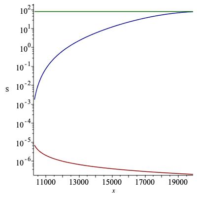
(a) $e=100$, $\lambda=1$

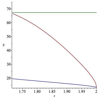
(b) $e=1$, $\lambda=1$

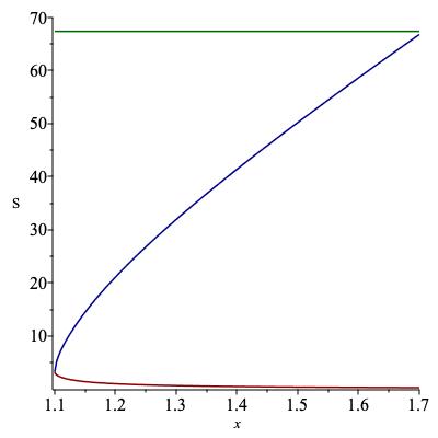
(c) $e=1$, $\lambda=100$

Figure 2: The entropy functions with $\kappa=\Lambda=r_{0}=1$. The green, red, and blue curves are the graphs of $S_{I}$, $S_{II}^{+}$, and $S_{II}^{-}$, respectively.

6.3.2 Option 2 Plots

In the ”Option 2 case” defined in the previous sections, Eq. (16) has one positive real roots (let us call it just $W_{0}^{2}$). In this case, transitions may appear as the thermodynamics is determined by the comparison of two solutions: the type I and the type II with root $W_{0}^{2}$. These two solutions will be characterized by their own entropy (Euclidean actions): let us call $S_{I}$ and $S_{II}$ the entropy of the type I solution and of the type II solution respectively. As in the option 1 case, $S_{I}$ and $S_{II}$ depends on all the parameters of the model, but we will emphasize the dependence on $v_{0}^{2}$.

Using the results from the previous subsection, we get the entropy function of the type II with a double root

$$S_{II}^{\text{(D)}}=S_{II}^{\text{(D)}}\left(x\right)=\frac{4\pi^{2}}{er_{0}^{2}\big{[}\lambda\kappa x+2-\lambda e^{2})\big{]}}\ .$$ (50)

The entropy function for the case with one positive and one negative roots equals to $S_{II}^{+}$. Also in this case, we plot together $S_{I}$ and $S_{II}$ as function of $x$ in two different cases (case 1: $e=1$, $\lambda=1$; case 2: $e=1$, $\lambda=100$) in order to show the differences between the situations in which the Higgs and Yang-Mills coupling are equal, and $\lambda$ is larger than $e$. In these three plots, $r_{0}$, $\Lambda$, and $\kappa$ will be fixed to 1. It should be emphasized that for a given set of the parameters $\{e,\lambda,\kappa,\Lambda,r_{0}\}$, the most preferred configuration can change as the square of the VEV varies. Interestingly, such a configuration changes continuously in Fig. (3(a)) whereas it changes in a discontinuous way, as can be seen in Fig. (3(b)) and (3(c)).

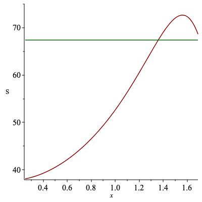
(a) $e=1$, $\lambda=1$

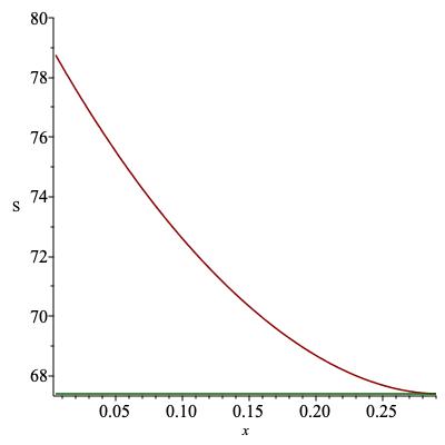
(b) $e=1$, $\lambda=100$

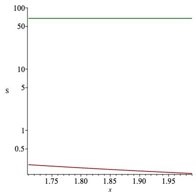
(c) $e=1$, $\lambda=100$

Figure 3: The entropy functions with $\kappa=\Lambda=r_{0}=1$. The green and red curves are the graphs of $S_{I}$ and $S_{II}$, respectively. The last two figures show two different regions for the same physical parameters. For the case with $e=1$ and $\lambda=100$, the interval $0.29<x<1.71$ is forbidden. In Fig. 3(a), the type I is favored for $x<1.359$ and the type II is favored for $x>1.359$. In Fig. 3(b), the type II always prevails, and in Fig. 3(c), the type I is always preferred.

7 Spin from Isospin and 4DQHE

The analysis of the Klein-Gordon equation reveals some crucial differences between the present non-Abelian versions of Nariai space-times and the well known Nariai space-times, which are solutions of the Einstein-Maxwell field equations [43, 44].

Let us begin this section with a very short review of the spin-from-isospin effect [45] [46] [47]. Roughly speaking, in the case of topologically non-trivial configurations that are not spherically symmetric but whose energy-momentum tensor is spherically symmetric the lack of spherical symmetry under spatial rotation is compensated by an internal transformation. This leads to a modification of the definition of the angular momentum, which in the usual example of non-Abelian $SU(2)$ monopoles reads:

$$\overrightarrow{L}\rightarrow\overrightarrow{J}=\overrightarrow{L}-\frac{1}{2}\overrightarrow{\tau}\ ,$$ (51)

where $\overrightarrow{L}$ is the orbital angular momentum and $\overrightarrow{\tau}$ are the $SU(2)$ generators entering in the ansatz of the gauge field. The new term in the definition of $\overrightarrow{J}$ is exactly related to the infinitesimal internal rotation needed to compensate the lack of spherical symmetry under spatial rotation. As it has been discussed in the original references [45] [46] [47] this leads scalar test fields moving in the background of this type of gauge fields to behave as Fermions. From the viewpoint of the Klein-Gordon equation this can be directly seen as follows. The non-Abelian flat Klein-Gordon operator reads (see [27] [29])

$$ds^{2}=-dt^{2}+dr^{2}+r^{2}\left(d\theta^{2}+\sin^{2}\theta d\phi^{2}\right)\ ,$$ (52)

$$D_{\mu}D^{\mu}=\left(\nabla_{\mu}-\left[A_{\mu},\cdot\right]\right)\left(\nabla^{\mu}-\left[A^{\mu},\cdot\right]\right)\Rightarrow$$

$$D_{\mu}D^{\mu}=\square_{2D}-\frac{\left(\overrightarrow{J}\cdot\overrightarrow{J}-c_{0}\right)}{r^{2}},$$ (53)

where $\square_{2D}$ is the two-dimensional D’Alembertian in the $t$ and $r$ coordinates and $c_{0}$ is a constant which depends on the representation of the test scalar field. Hence, Eq. (53) explains in a very simple way the effect of the “need to compensate” the lack of spherical symmetry with an internal rotation: the centrifugal barrier (which is the term that goes as $1/r^{2}$ for large $r$) is modified. Obviously, it is precisely from the centrifugal-barrier like term that one usually reads the spin of the “test fields”. A quite trivial (but useful as we will now show) observation is the following: the $1/r^{2}$ factor which multiplies $\overrightarrow{J}\cdot\overrightarrow{J}$ arises because of the $r^{2}$ term in front of the two-sphere in the metric in Eq. (52). Now, we are ready for an important question:

What happens if in the spherically symmetric space-time of our interest (sourced by a non-Abelian soliton) in front of the two-sphere we have just a constant instead of the coordinate-dependent factor $r^{2}$? What happens to the spin-from-isospin effect?

Eq. (53) suggests an intriguing answer: the (modified) centrifugal barrier becomes a term that does not depend on $r$ at all: such a term possesses discrete degenerate energy levels (as it is proportional to $\overrightarrow{J}\cdot\overrightarrow{J}$) with an energy gap proportional to the (homogeneous) magnetic flux. In other words, when in front of the two-sphere we have a constant instead of $r^{2}$ the “spin-from-isospin” term is replaced by the typical Hamiltonian which is used to describe the QHE in higher dimensions (see in particular, [30] [31]). We will now show that this is indeed the case, and that the degeneracy of the energy levels of the non-Abelian Klein-Gordon equation changes dramatically when passing from the type I to the type II solutions: such an effect is a genuine non-Abelian fingerprint of the present families of gravitating solitons.

Let us consider scalar test fields $\Psi^{a}$ $(a=1,2)$, which transforms like a two-component vector, in our background space-time. The field equation is given by

$$D^{2}\Psi-m^{2}=0\ ,$$

where $m$ is the mass of the scalar fields. Note that the Yang-Mills field associated with our solution satisfies

$$\nabla^{\mu}A_{\mu}=0\ ,\qquad A^{\mu}A_{\mu}=-\frac{2X_{0}^{2}}{L^{2}F_{0}}\mathbf{1}_{2\times 2}\ .$$

The Klein-Gordon equation can be written as

$$\nabla^{2}\Psi-m^{2}\Psi+2A^{\mu}\nabla_{\mu}\Psi+A^{\mu}A_{\mu}\Psi=0\ .$$

Explicitly, it can be written as

$$\Delta_{(u,v)}\Psi+\Big{[}\frac{1}{F_{0}L^{2}}\big{(}\vec{L}-X_{0}\vec{\tau}\big{)}^{2}+\frac{X_{0}^{2}}{F_{0}L^{2}}-m^{2}\Big{]}\Psi=0\ ,$$

where $\hat{L}=\hat{L}_{i}\tau_{i}$ for the standard angular momentum operators $\hat{L}_{i}$, and $\Delta_{(u,v)}$ is the 2 dimensional D’Alembertian operator given by

$$\Delta_{(u,v)}=-\frac{2}{F_{0}y_{0}}\partial_{u}\partial_{v}\ .$$

The eingenfunction of this operator has the form of

$$\Psi=e^{au+bv}\Psi_{0}\ ,$$ (54)

with the eigenvalue $-2ab/F_{0}y_{0}$, for arbitrary constants $a$ and $b$, and a constant doublet $\Psi_{0}$.

7.1 Differences between type I and type II non-Abelian solitons

In the case of the type I non-Abelian gravitating solitons one can compute the sum of the orbital and isospin angular momenta through a standard procedure. In particular, the eigenvalues of the spin-orbit coupling can be obtained by

$$\vec{J}^{2}=\Big{(}\vec{L}+\frac{1}{2}\vec{\tau}\Big{)}^{2}=\vec{L}^{2}+\frac{1}{4}\vec{\tau}^{2}+\vec{L}\cdot\vec{\tau}\quad\Longrightarrow\quad\vec{L}\cdot\vec{\tau}=\vec{J}^{2}-\vec{L}^{2}-\frac{1}{4}\vec{\tau}^{2}$$ (55)

which gives the eigenvalues of the coupling operator $\vec{L}\cdot\vec{\tau}$

$$j(j+1)-l(l+1)-\frac{1}{2}\cdot\Big{(}\frac{1}{2}+1\Big{)}\ .$$

Thus, the part of the Hamiltonian which results in a spin-isospin effect

$$H_{\text{spin-isospin}}=\frac{1}{F_{0}L^{2}}\big{(}\vec{L}-X_{0}\vec{\tau}\big{)}^{2}$$ (56)

has the same degeneracy of the physical system as the usual spin-orbit couplings when $X_{0}=1/2$. It gives a very similar behavior of the Hamiltonian of the four dimensional quantum hall effect proposed in [30],

$$H_{\text{QHE}}=\frac{1}{2MR^{2}}\sum_{a<b}\Lambda_{ab}^{2}\ ,$$

where $\Lambda_{ab}=-i\big{(}x_{a}D_{b}-x_{b}D_{a}\big{)}$. Here, $F_{0}L^{2}$, the denominator of (56), plays the same role as the radius of the orbit in the system with QHE.

On the other hand, in the gravitating solitons of type II (In the case with $X_{0}\neq 1/2$ and a non-trivial Higgs field) the (would be) total angular momentum $\overrightarrow{J}$ becomes

$$\overrightarrow{J}=\vec{L}-X_{0}\vec{\tau}$$

with a real coefficient $X_{0}$ different from $1/2$ (as, generically, $X_{0}$ is not even a rational number: see Eqs. (13) and (16)). The most dramatic effect manifests itself in the degeneracy of the energy level associated to the operator (56). This can be understood easily looking at the standard manipulations in Eq. (55) in the case in which $X_{0}$ is a generic real number:

$$\overrightarrow{J}=\vec{L}-X_{0}\vec{\tau}\ ,\ and\ \ X_{0}\neq 1/2,\ 0\qquad\Longrightarrow\qquad[J_{i},J_{k}]\neq\varepsilon_{ikl}J_{l}.$$ (57)

Although one may still hope to find a rigorous definition of the “total angular momentum $\overrightarrow{J}$” with $X_{0}$ a real number, it is clear that one should not expect that the spectrum of the above “spin-from-isospin operator” $H_{\text{spin-isospin}}$ in Eq. (56) is still related to the combination

$$j\left(j+1\right)\ ,\$$

$$j=l+X_{0}\ .$$

The reason is that Eq. (57) suggests that the eigenvalues of $H_{\text{spin-isospin}}$ depend on $l$ (related to the eigenvalues of $\vec{L}$) and $s$ (related to the eigenvalues of $\vec{\tau}$) separately (and therefore the degeneracy is expected to be lower than in the case with $X_{0}=1/2$ when the eigenvalues only depend on $j$). Consequently, the non-Abelian Klein-Gordon equation associated to the type II gravitating merons should have energy levels with a different degeneracy than in the case of the type I gravitating solitons.

This has the following potential consequence. A multi-Fermionic system (charged under the gauge group) living in the type I gravitating solitons (in the approximation in which these Fermions can be considered as test fields) would be subject to a Hamiltonian with many of the features of the 4D QHE (as it has been explained here above). The same multi-Fermionic system would perceive a Hamiltonian with very different degeneracies in the type II gravitating solitons. Therefore, if there is a semiclassical transition from one family to the other the multi-Fermionic system would suddenly be subject to a different QHE-like Hamiltonian with completely different degeneracies. We hope to come back on the fascinating physical properties of these scenarios in a future publication.

8 Conclusions

In this article, we constructed the first two analytic families of globally regular non-Abelian gravitating solitons in the Einstein-Yang-Mills-Higgs theory in (3+1)-dimensions with the Higgs field in the adjoint representation (however, the case in which the Higgs field is in the fundamental is very similar). The space-time metric is of Nariai type in both cases. The Yang-Mills fields are of meron type (namely, proportional to a pure gauge: $A_{\mu}=X_{0}U^{-1}\partial_{\mu}U$ for some parameter $X_{0}$) for both families. On the other hand, while in the first family (called type I in the main text) of non-Abelian gravitating soliton $X_{0}=1/2$ (as in all the known examples of merons available so far) and the Higgs field is trivial, in the second family (type II) $X_{0}\neq 1/2$ and the Higgs field is non-trivial (to the best of the authors knowledge, this is the first example of meron solutions with $X_{0}\neq 1/2$). We have compared these two families of globally regular gravitating solitons by computing the Euclidean action of both types. This allows to determine when type II solitons (with a non-trivial Higgs and $X_{0}\neq 1/2$) are favored over type I solitons and viceversa. It turns out that the most favored configuration is determined in a sensitive way depending on the parameters of the model. Even for a given set of the parameters other than $x=v_{0}^{2}$, the most preferred configuration changes continuously or discontinuously as $x$ varies. In order to disclose the differences between type I and type II gravitating solitons we analyzed the non-Abelian Klein-Gordon equation for a test scalar field minimally coupled to the non-Abelian fields sourcing the gravitating solitons themselves. The Klein-Gordon equation is able to detect very neatly the difference between type I and type II solitons (despite the fact that the space-time metric is similar in both cases). The Klein-Gordon equation can be written as the sum of a two-dimensional D‘Alambert operator plus one of the Hamiltonians which has been proposed in the literature to describe the four-dimensional Quantum Hall Effect (QHE): the difference between type I and type II solutions manifests itself in a difference between the degeneracies of the corresponding energy levels. This opens the very intriguing perspective to analyze the “many-body” wave functions of multi-Fermionic systems minimally coupled to the regular meronic fields of type I and type II solutions (in the test field limit in which these Fermions do not modify substantially the space-time metric). The idea would be to distinguish type I and type II solutions by looking at the degeneracy of the corresponding Landau Levels. We will return to this very interesting issue in a future publication.

References

• [1] S. Coleman, Classical lumps and their quantum descendants, In Erice subnuclear physics, page 297, 1975.
• [2] A. Actor, Rev. Mod. Phys. 51, 461โ€“525 (1979).
• [3] R. Rajaraman, Solitons and Instantons, North-Holland, 1982.
• [4] N.ย Manton and P.ย Sutcliffe, Topological Solitons, (Cambridge University Press, Cambridge, 2007).
• [5] A. Balachandran, G. Marmo, B. Skagerstam, A. Stern, Classical Topology and Quantum States, World Scientific (1991).
• [6] A. Vilenkin, E. P. S. Shellard, Cosmic Strings and Other Topological Defects, Cambridge University Press (2000).
• [7] R. Bartnik, J. McKinnon, Phys.Rev.Lett. 61, 141โ€“144 (1988).
• [8] M.S. Volkov, D.V.Galโ€™tsov, JETP Lett. 50, 346โ€“350 (1989); Phys. Lett. B 341, 279โ€“285 (1995); Sov. J. Nucl. Phys. 51, 747โ€“753 (1990).
• [9] H.P. Kunzle, A.K.M. Masood ul Alam, Journ. Math. Phys. 31, 928โ€“935 (1990).
• [10] P. Bizon, Phys.Rev.Lett. 64, 2844โ€“2847 (1990).
• [11] M.S. Volkov, D.V.Galโ€™tsov, Phys. Rept. 319, 1-83 (1999).
• [12] P. Breitenlohner, D. Maison, G. Lavrelashvili, Class.Quant.Grav. 21 (2004) 6, 1667-1684.
• [13] P. Breitenlohner, P. Forgacs, G. Lavrelashvili, Nucl.Phys.B 383 (1992) 357-376; Nucl.Phys.B 442 (1995) 126-156.
• [14] P. Bizon, Acta Phys.Polon.B 25 (1994) 877-898.
• [15] E. Winstanley, Springer Proc.Phys. 208 (2018) 39-46, Contribution to: KSM 2015, 39-46; e-Print: 1510.01669 [gr-qc].
• [16] J. E. Baxter, E. Winstanley, Phys.Lett.B 753 (2016) 268-273.
• [17] B. L. Shepherd, E. Winstanley, Phys.Rev.D 93 (2016) 6, 064064; JHEP 01 (2017) 065.
• [18] A. H. Chamseddine, M. S. Volkov, Phys. Rev. Lett. 79, 3343 (1997).
• [19] T. Ioannidou, B. Kleihaus, J. Kunz, Phys. Lett. B 600 (2004) 116-125; ibid 643 (2006) 213-220.
• [20] M. Wachla, Phys.Rev. D 99 (2019) 065006.
• [21] S.-B. Gudnason, M. Nitta, N. Sawado, JHEP 1512 (2015) 01.
• [22] V. de Alfaro, S. Fubini, G. Furlan, Phys. Lett. B 65 (1976) 163.
• [23] C.G. Callan Jr., R.F. Dashen, D.J. Gross, Phys. Rev. D 19 (1979) 1826; Phys. Rev. D 17 (1978) 2717; Phys. Lett. B 66 (1977) 375.
• [24] J. Glimm, A.M. Jaffe, Phys. Rev. Lett. 40 (1978) 277.
• [25] F. Lenz, J.W. Negele, M. Thies, Phys. Rev. D 69 (2004) 074009.
• [26] P. Cordero, C. Teitelboim, Ann. Phys. 100 (1976) 607.
• [27] F. Canfora, F. Correa, A. Giacomini, J. Oliva, Phys.Lett.B 722 (2013) 364-371.
• [28] F. Canfora, S. H. Oh, P. Salgado-Rebolledo, Phys.Rev.D 96 (2017) 8, 084038.
• [29] F. Canfora, A. Gomberoff, S. H. Oh, F. Rojas, P. Salgado-Rebolledo, JHEP 06 (2019) 081.
• [30] S. C. Zhang, J. P. Hu, Science 294, 823 (2001); J. P. Hu, S. C. Zhang, arXiv:cond-mat/0112432.
• [31] D. Karabali and V. P. Nair, Nucl. Phys. B641, 533 (2002); , Nucl. Phys. B679, 427 (2004); Nucl. Phys. B697, 513 (2004); J. Phys. A 39, 12735 (2006).
• [32] M. Fabinger, J. High Energy Phys. 05 (2002) 037.
• [33] Y. X. Chen, B. Y. Hou, B. Y. Hou, Nucl. Phys. B638, 220 (2002).
• [34] H. Elvang, J. Polchinski, The quantum Hall effect on R4, arXiv:hep-th/0209104.
• [35] B. A. Bernevig, C. H. Chern, J. P. Hu, N. Toumbas, S. C. Zhang, Ann. Phys. (Amsterdam) 300, 185 (2002); B. A. Bernevig, J. P. Hu, N. Toumbas, S. C. Zhang, Phys. Rev. Lett. 91, 236803 (2003).
• [36] G. Meng, J. Phys. A 36, 9415 (2003); V. P. Nair, S. Randjbar-Daemi, Nucl. Phys. B679, 447 (2004); A. Jellal, Nucl. Phys. B725, 554 (2005).
• [37] Kraus, Y. E., Ringel, Z. & Zilberberg, Phys. Rev. Lett. 111, 226401 (2013).
• [38] M. Lohse, C. Schweizer, H. M. Price, O. Zilberberg, I. Bloch, Nature 553, 55โ€“58 (2018).
• [39] O. Zilberberg, S. Huang, J. Guglielmon, M. Wang, K. P. Chen, Y. E. Kraus, M. C. Rechtsman, Nature 553, 59โ€“62 (2018).
• [40] A. Sen, JHEP 09, 038 (2005).
• [41] Jin-Ho Cho and Soonkeon Nam, JHEP 03, 027 (2008).
• [42] F. Canfora, Phys.Rev.D 76 (2007) 084012.
• [43] B. Bertotti, Phys. Rev. 116, 1331 (1959).
• [44] I. Robinson, Bull. Acad. Pol. Sci. Ser. Sci. Math. Astron. Phys. 7, 351 (1959).
• [45] R. Jackiw, C. Rebbi, Phys. Rev. Lett. 36 (1976) 1116.
• [46] P. Hasenfratz, G. โ€™t Hooft, Phys. Rev. Lett. 36 (1976) 1119.
• [47] A.S. Goldhaber, Phys. Rev. Lett. 36 (1976) 1122.
• [48] L. F. Abbott and S. Deser, Phys. Lett. 116B, 259 (1982).