Flat: An Optimized Dataflow for Mitigating Attention Bottlenecks

Abstract

Attention mechanisms, primarily designed to capture pairwise correlations between words, have become the backbone of machine learning, expanding beyond natural language processing into other domains. This growth in adaptation comes at the cost of prohibitively large memory requirements and computational complexity, especially at higher number of input elements. This limitation is due to inherently limited data reuse opportunities and quadratic growth in memory footprints, leading to severe memory-boundedness and limited scalability of input elements. This work addresses these challenges by devising a tailored dataflow optimization, called Flat, for attention mechanisms without altering their functionality. This dataflow processes costly attention operations through a unique fusion mechanism, transforming the memory footprint quadratic growth to merely a linear one. To realize the full potential of this bespoke mechanism, we propose a tiling approach to enhance the data reuse across attention operations. Our method both mitigates the off-chip bandwidth bottleneck as well as reduces the on-chip memory requirement. Flat delivers 1.94$\times$ (1.76$\times$) speedup and 49% and (42%) of energy savings compared to the state-of-the-art Edge (Cloud) accelerators with no customized dataflow optimization. When on-chip resources are scarce (20 KB-200 KB), Flat yields, on average, 1.5$\times$ end-to-end latency reduction across a diverse range of conventional attention-based models with input sequence lengths ranging from 512-token to 64K-token. Our evaluations demonstrate that state-of-the-art DNN dataflows applied to attention operations reach the efficiency limit for inputs above 512 elements. In contrast, Flat unblocks transformer models for inputs with up to 64K elements.

1 Introduction

Attention mechanisms, the key building block of transformer models, have enabled state-of-the-art results across a wide range of machine learning (ML) tasks—from natural language processing (NLP) [89, 17, 52], to object detection [109, 6, 81], image classification [106, 27, 99, 108], image generation [7, 65, 21], and music synthesis [34, 33]. This exponential growth of transformer models are expected to serve as the foundation of a new bread of machine learning models in the upcoming years. A key attribute of attention-based models is the sequence length ($N$) defining the number of input elements for which a pairwise correlation scores is computed. Intuitively, increasing sequence length enables the attention-based models to better capture the context of input sentences or the relation between image segments. The demand for leveraging long-sequence (e.g. $N=8K$ to $N=69K$) attention-based models has already emerged in ML community [86], beyond natural language understanding [69] into protein folding [14] and text summarization [46] and audio generation [56]. Employing long sequences is pivotal in these algorithms because the property of input emerges from the global context. For example, two proteins may look identical if we examine identical sequence fragments, but when the entire sequence is considered, the differences in their function arise. We observe an analogous phenomenon in text summarization, where context can drastically alter the meaning of the selected text subset. In that instance, the subset represents a shorter sequence while the entire context refers to the full-length one.

Compared to existing neural network accelerators [10, 9, 20, 77, 66, 103], architecting accelerators for attention-based models poses different design challenges, attributed to their soaring demand for on-chip memory and compute complexities. Recent accelerators for attention-based models [29, 30] have mainly relied on algorithmic optimizations, often with negative repercussion on model accuracy. Algorithmic techniques in practice include sparsification or compression [93, 42, 13, 14, 79, 65, 67, 12, 5, 16, 46, 72, 85, 17, 69, 55, 102] and/or leveraging lossy approximation [30, 29, 92].

In this work, we identify that the conventional dataflow/mapping methods for CONV and FC layers [62, 20, 40, 9] are inadequate for attention layers. This is because the main operators within attention layers exhibit distinct compute and memory characteristics posing notable bottlenecks on off-chip memory bandwidth compared to CONV and FC. We identify the following challenges in devising dataflow optimizations for attention layers:

1. Significantly low operational intensity. Inherently low data reuse in activation-activation operators significantly reduces the operational density of such operators in attention layers. This inherently low operational density subsequently makes the activation-activation operators fundamentally memory-bound. While prior work on intra-operator dataflow optimization, such as loop transformation and scheduling techniques [62, 10, 20, 64, 50, 48], targets CONV and batched FC operators by leveraging the ample intrinsic data reuse, which are not well-suited for activation-activation operators lacking data reuse opportunity.

2. Complex many-to-many operators. The main attention operators have many-to-many relation, obscuring opportunities to use operator fusion [61] in attention operators. That is because operator fusion in conventional ML compilers [8, 71, 26] mainly target operations such as CONV and FC with one-to-one (i.e. element-wise) relation.

3. Prohibitively large intermediate tensors. The size of intermediate tensors in attention layers grows quadratically—$\mathcal{O}(N^{2})$) [89, 17, 52, 93, 42, 13, 14]—with the sequence length. This quadratic growth imposes a significant pressure on on-chip memory capacity and prohibits opportunities to store the intermediate results on-chip and improve the compute utilization, a common practice in CNN accelerators [9].

This paper fundamentally tackles the challenges associated with attention layers by devising a first in its class many-to-many inter-operator dataflow optimization mechanism, called Fused Logit Attention Tiling. This optimization particularly fuses multiple many-to-many tensor operator, while systematically preserving their inter-operator data dependencies, leading to a significant reduction on off-chip memory bandwidth pressure. In addition, to fully realizing the performance benefit of this inter-operator fusing mechanism, Flat performs a new tiling approach across the fused operators. This tiling enables efficient staging of quadratically growing intermediate tensors of attention operations on tight-budgeted on-chip memories, leading to higher performance and energy savings and elevates the scalability of transformer models up to 64K inputs. These benefits are unlocked with only modest hardware changes, integrating into a platform deployable on off-the-shelf DNN accelerators. In summary, this paper presents the following specific contributions for attention-based models:

• We systematically study the operational intensity of different operators within attention layers and characterize the fundamental roadblocks imposed by limited hardware resources to improve the overall realized performance of attention accelerators (§ 3).

• Based on the resulting findings, we explore fusion opportunities between different operators in attention layers and justify our proposed many-to-many inter-operator fusion (§ 4). While beneficial, this fusion inflicts a fundamental challenge of preserving the inter-operator data dependencies, imposed by the softmax operation. To address, we expound our tailored dataflow optimization approach for attention layers, enabling higher data reuse of the quadratically growing intermediate attention tensors from low-capacity but high-bandwidth on-chip memory. We show that this dataflow optimization efficiently mitigates the pressure on off-chip memory bandwidth, leading to a higher performance and energy efficiency in accelerators (§ 5).

• We develop a map-space exploration framework to efficiently search for optimal loop orders across fused operators and tiling sizes. This framework optimizes performance metrics of interest subject to different hardware resource constraints, such as number of processing elements and on-chip memory capacity (§ 6).

We evaluate Flat on a variety of Attention-based models, including BERT [89], TrXL [52], FlauBERT [53], T5 [70], and XLM [52], for both Edge and Cloud accelerators. Compared to a range of state-of-the-art dataflow optimizers, Flat delivers 1.75$\times$ and 1.65$\times$ speedup and 44$\%$ and 55$\%$ energy savings for recent Edge and Cloud accelerators, respectively. When on-chip resources are scarce (in the order of 10KB-100KB), Flat yields 1.5x end-to-end latency reduction and 1.4x end-to-end energy savings for the Attention-models with conventionally-sized input sequence length (512-token). Furthermore, our results show that while the conventional DNN dataflow optimizers for attention operations bumps up against the efficiency limit for inputs above 512 tokens, our dataflow optimization tailored for attention operations unblocks the scalability of transformer models for significantly larger input sizes, up to 64K tokens.

2 Background on Attention-Based Models

Terminology. Transformer models [89, 53, 82] generally share similar architectures. In a top-down view (Fig. 1), an attention-based “model” comprises multiple (often identically parameterized) attention “blocks”. An attention block comprises multiple “layers”: an attention layer, a normalization layer, followed by multiple (typically two) fully connected layers. Finally, each layer comprises one or more “operations” or “operators”.

Computation operators. The attention mechanism measures how closely two tokens are related in an input sequence. Each token in the input sequence is represented as a vector of dimension $D$, each sequence has $N$ tokens, and an input batch to an attention layer comprises a batch of $B$ sequences; thus the input to the attention layer is a tensor of dimension $[B,N,D]$. Fig. 1 (bottom) highlights the flow of a single token vector (of dimension $D$) through the attention mechanism. Step , three vectors are derived for each token’s vector in the input: called Key (K), Query (Q), Value (V). This is achieved by multiplying the input tensor with learnable weight matrices. Attention mechanisms often use multiple heads to generate $H$ such K, Q, V vectors for each token vector in the input. Thus each of K, Q, V generates a tensor of dimension $[B,H,N,d]$. Step , we compute the logits score (L) which captures how strongly each token is related to each other token in the sequence. This is done by a ($d$-dim) dot product of each vector of the key with the corresponding vector of the query. Each dot product yields a single scalar score, but this score is computed for each token against all other tokens in the sequence yielding an output tensor of dimension $[B,H,N,N]$. Step , the logits scores then needs to be normalized. While there are several normalization functions, they all share key traits. The normalization is carried out across a row of $N$ logits scores in each sequence. To generate a row of $N$ normalized scores, the normalization operator reads $N$ input scores, performs a reduction of these $N$ scores, and scales each of the $N$ input scores by the reduced value. We use softmax since it is the most commonly used normalization function. Step , involves performing a weighted sum of the value vectors with the corresponding weights from the logits, which yields an output tensor $[B,H,N,d]$. Finally, step concatenates the attention outputs from the $H$ heads and with its weight matrix computes a output tensor $[B,N,D]$. These complete an attention layer.

This can be represented succinctly as the computational graph in Fig. 1, comprising the following operators: i) Query (Q), Key (K), and Value (V) operators that perform a projection of the input tensor, ii) Logit (L) and Attend (A) operators that compute the logits scores and weighted-sum of values respectively, and iii) Output (O) operator that performs an output projection. We categorize them into two: (i) activation-weight operators (Q, K, V, O), which operate on activation tensors (from previous operators) and weight tensors (model parameters) and perform a GEMM computation as conventional fully connected operators (FCs), and ii) activation-activation operators (L, A), which operate on two activations from different previous operators and perform a GEMM computation. The L and A operators often dominate the latency and power consumption while running the model [29], and even more so at long sequence lengths, as shown in our evaluations (Fig. 14).

2.1 DNN Accelerators - Performance Considerations

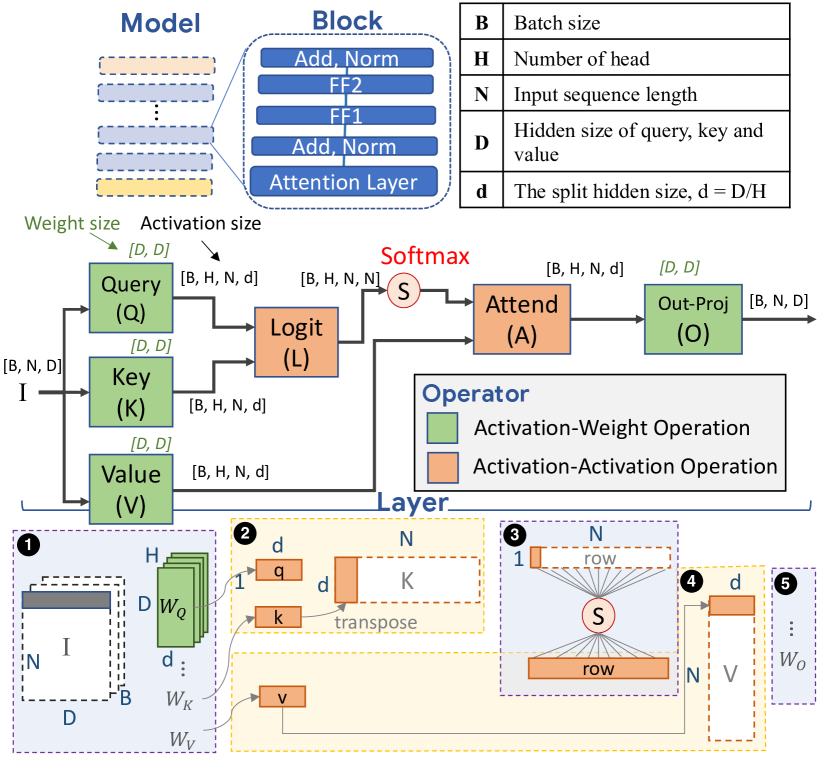
Fig. 1: The structure of attention-based models. Green matrix notation shows the size of weight tensors; black matrix notation shows the size of activation tensors; Softmax is applied on output of Logit.

We consider spatial DNN accelerators [9, 48, 25] in this work (Fig. 15 provides more details). We discuss the key factors that determine the realized performance when running a DNN model on an accelerator with specific hardware resources (PEs, on-chip memory size, and off-chip memory BW).

Operational intensity | Roofline performance. Operational intensity is a proxy metric to gauge the maximum possible performance of an individual operator given a set of hardware resources. The operational intensity of an operator is defined as the number of arithmetic operations divided by the number of memory accesses. A lower operational intensity implies an operator has fewer opportunities for data reuse and is more likely to be memory bandwidth(BW)-bounded. This directly decides the roofline (or best achievable) performance of the operator on the underlying accelerator.

$$\begin{gathered}\mathcal{I}=\frac{\#\ \mathrm{of}\ \mathrm{Operations}}{\#\ \mathrm{of}\ \mathrm{Memory}\ \mathrm{Accesses}}\end{gathered}$$ (2)

Dataflow | Realized performance. Dataflow refers to the mechanisms to stage data from the off-chip memory through the on-chip memory hierarchy to the compute PEs, over space and time [48]. It determines the actual achieved performance. Since memory access is often the bottleneck in executing DNN operators [83], the dataflow exposes data reuse opportunities across operands that can be exploited in hardware via buffering and data forwarding/broadcast [48]. Formally, the dataflow encompasses: (i) tiling (how tensors are sliced, stored and fetched across the memory hierarchy), (ii) compute order (order in which loop iterations are performed), and (iii) parallelism (how compute is mapped across PEs spatially). The dataflow along with specific tile sizes is often called a mapping [50, 48].

3 Challenges with Running Attention Layers

3.1 Challenge 1: Low Operational Intensity of L/A

Activation-Weight operators (Q/K/V/O). Following the notation in Fig. 1, the number of operations in these operators is $\mathcal{O}(BND^{2})$. The number of memory accesses for the input (activations), weight (parameters), and output (activations) tensors are $\mathcal{O}(BND)$, $\mathcal{O}(D^{2})$, $\mathcal{O}(BND)$, respectively. Therefore the operational intensity is $\mathcal{O}(\frac{BND^{2}}{BND+D^{2}+BND})$. We see that increasing the batch size (B) can increase the operational intensity—the same weight value can be reused by multiple activations, leading to lower BW pressure. This is a typical technique used in activation-weight operators (e.g., CONV and FC, the staple in most DNN models) as it makes better use of the scarce memory bandwidth in accelerators and enables higher utilization of the provisioned compute FLOPs, leading to improved throughput. The specific mechanism to exploit the operational intensity is called dataflow [9, 48].

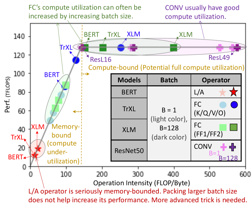
Fig. 2: Roofline analysis on TPU-v3 [39] for operators in BERT(-base) [89], TrXL(-large) [17], and XLM (xlm-mem-en) [52], and ResNet50 [31] using sequence length = 512.

Activation-Activation operators (L/A). For L and A operators, the number of operations is $\mathcal{O}(BN^{2}D)$. The number of memory access for the two input-activations and the output-activations are $\mathcal{O}(BND)$, $\mathcal{O}(BND)$, $\mathcal{O}(BN^{2})$, respectively. Therefore the operational intensity is $\mathcal{O}(\frac{BN^{2}D}{2BND+BN^{2}})$. Embedding size (D) is decided by the model, and sequence length (N) is decided by the application. Furthermore, multi-head attention is an often-used variant of the attention mechanism: it leads to higher accuracy in many tasks [89]. It splits the output of the Q/K/V operator along a hidden dimension, reshaping it from size [N, D] to [H, N, d], where d=D/H. The operational intensity of L, A becomes $\mathcal{O}(\frac{BN^{2}D}{2BND+BHN^{2}})$. For these operators, one can not simply increase the batch size to increase the operational intensity.

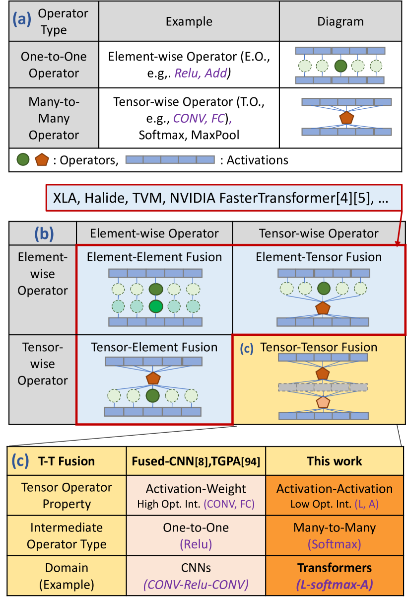
Fig. 3: (a) Type of Operator, (b) Type of Operator-Fusion, and (c) Type of Tensor-Tensor Fusion.

Roofline analysis. To quantitatively demonstrate the effect of operation intensity across different operators, we show the roofline analysis of operators of three common attention-based models [89, 17, 52] and a widely used CNN network ResNet50 [31] on TPU-v3 [39] in Fig. 2. We can see that CONV operators lie in the compute-bound region. FC operators scatter across both memory and compute bound region; however, with the increase in batch size, their operation intensity increases and can become compute-bound. This demonstrates why batching is a popular technique for FC layers. In contrast, L and A operators sit at memory-bound and low-performance region, and batch size increase is not effective in these operators (Fig. 2).

In summary, low operational intensity of the individual L/A operators makes them fundamentally memory-bound, and any dataflow/mapping exploration at the individual operator level cannot further improve performance.

3.2 Challenge 2: Complexity of Op Fusion for L/A

Given the low operational intensity for L/A operators, fusion is an attractive technique to stage the intermediate tensor data on-chip and leverage the higher on-chip memory bandwidth. Operator fusion is an optimization that schedules back-to-back operators together such that the producer’s output directly feeds the consumer, thus avoiding materialization of full intermediate tensor in memory. By avoiding off-chip data movement of the intermediate tensor, we can use the higher on-chip bandwidth to enable improved performance for the fused operator (as opposed to executing the operators individually).

When exploring operation fusion opportunities, we can either fuse among Element-wise Operators (E.O.) or Tensor-wise Operators (T.O.), as shown in Fig. 3. Element-Element fusion (E-E) is the simplest fusion optimization. With increased interest in operation fusion, more ML compilers/frameworks today support Tensor-Element (T-E) or Element-Tensor (E-T) fusion [8, 4, 47, 26, 71] where MatMul operators (i.e., CONV or FC) are often fused with element-wise operators (such as ReLu or Add), reshapes, or shuffling operators [61]

However, Tensor-Tensor Fusion (T-T) is not done automatically. The key reason is that T.O. is a many-to-many operator (Fig. 3(a)). While it is often straightforward and a simple engineering exercise to fuse a T.O. with one-to-one operator like E.O., how to fuse many-to-many with other many-to-many and whether it is beneficial to fuse them is still a research question [61]. Indeed, DNNFusion [61] which studied T-T as recently as PLDI 2021, reported it to be either too complicated or unprofitable. The key reason is that the additional complexity to maintain dependence and stage data (grey intermediate data as shown in Fig. 3(b)) could end up negatively impacting register and cache usage [61].

Some previous research papers [2, 96] have discussed Tensor-Fusion in CNNs with the fusion pattern T-(one-to-one)-T such as CONV-Relu-CONV and shown huge potential gain with a well-designed inter-operator dataflow for Tensor-Fusion. This is highlighted in Fig. 3(c). However, Tensor-Fusion for attention-based models has not been explored to date, to the best of our knowledge. The complexity of its fusion pattern, T-(many-to-many)-T, makes it much more challenging than for CNNs.

To address this challenge, we design a specialized inter-operator dataflow that not only considers the data dependency of two large tensor operators but also tackles the additional complex data dependency incurred by the many-to-many intermediate activation (§ 5.2).

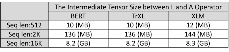
Fig. 4: Intermediate tensor size between L and A operators in BERT(-base) [89], TrXL(-large) [17], and XLM(xlm-mem-en) [52].

3.3 Challenge 3: Tensor Footprint of L/A

There is one other challenge that is unique to L/A when considering Tensor-Fusion—namely a quadratic intermediate tensor footprint. From Fig. 1 we can calculate the intermediate tensor between L and A operators has size $\mathcal{O}(BHN^{2})$ (M-Gran in Table 1). This footprint grows quadratically with sequence length, and exceeds 8GB (exceeding the viable on-chip memory in many data-center class accelerators [39, 88]) beyond sequence lengths of 16K (Fig. 4). As NLP tasks with larger sequence lengths become popular [46, 69, 14], the technique of keeping the entire intermediate tensor on-chip is not scalable. To address this, we propose a tiling technique for our fused operator that enables controlling the active memory footprint based on the on-chip memory constraint.

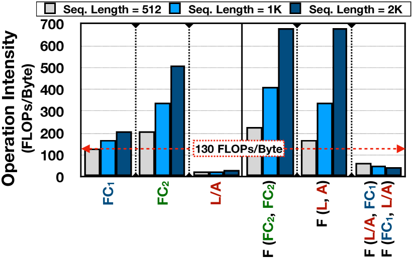
Fig. 5: Potential of Tensor-Tensor Fusion. The operation intensity ($\mathcal{I}$) of single and fused operators in attention layers in TrXL(-large) [17] using batch size=1. The notations are from Fig. 1. F(X, Y) implies fusion between X and Y operator. The red dashed bar indicates the minimum operation intensity for the operator to become compute-bound. FC₁ and FC₂ indicate operator K/Q/V/O and FF1/FF2, respectively. F(L/A, FC₁) specifies fusion between “A” and “O”, whereas F(FC₁, L/A) expresses the fusion between “Q-L”, “V-A”, and “K-L”.

4 Flat Dataflow Concept

We design a specialized dataflow strategy, Fused Logit Attention Tiling (Flat), targeting the two memory BW-bound operators in the attention layer, L and A. Flat includes both intra-operator dataflow and a specialized inter-operator dataflow, executing L and A in concert.

4.1 Identifying Tensor Fusion Opportunity

Fig. 5 plots the operation intensity ($\mathcal{I}$) of single and fused operators in attention layers of an attention-based model [17]. The dotted line marks the operation intensity threshold (ridge point) from memory to compute boundedness in TPU-v3 [39]. We observe that for FC-based operators (K/Q/V/O), the operational intensity is sufficient to be compute-bound, while for L/A it is low (as we had also observed via Fig. 2). However, after fusing L and A (f(L, A)), the effective operational intensity (of the fused operator) is higher. This motivates us to explore L and A fusion.

Why not fuse other operators? We did not fuse other operator pairs such as f(Q, L), f(A, O), or f(V, A), for three reasons. (1) The operational intensity is often sufficient and can be increased by leveraging batch size to reach compute-bound (Fig. 2). (2) Fusing two FCs (f(FC, FC)) can achieve higher operational intensity; however since the operator is already compute-bound, there is not much value in leveraging fusion (and the additional complexity). (3) We often need finer-granularity dataflow schemes to fit fused operator tensors on-chip; however fusing two activation-weight computation (f(FC, FC)) can trade-off (weight) reuse opportunity and may reduce actual achievable performance (§ 5.3).

Why not fuse multiple operators? We did not fuse multiple operators such as f(L, A, O) or f(K, L, A) for two reasons. (1) Fusing L/A with FC such as f(A, O) or f(K, L) can drop the potential performance of FCs compared to their single operator performance (Fig. 5). (2) The more operators we fuse, the more data we need to stage partially on-chip. Since the on-chip memory is often extremely limited, we need to execute the fused operators at a much finer granularity, which may lead to a degradation in achievable performance (§ 5.3). With these analyses, we decide to fuse only L and A.

4.2 Challenges with Tensor Fusion Implementation

Fusing L and A operators introduces two key challenges that we discuss here. § 5 presents implementation details.

Challenge 1: Respecting data dependencies across operators. Fusing L and A causes its unique challenge of data dependency owing to the many-to-many Softmax operation between them (§ 3.2). Softmax requires a reduction along a specific dimension of the tensor before scaling individual elements. Arbitrary inter-loop tiling as employed by prior CONV/FC fusion techniques [2, 96] violates this data dependency constraint.

Challenge 2: Effectively handling large intermediate tensors that do not fit in on-chip memory. Recall that the intermediate tensor between L and A has size $\mathcal{O}(BHN^{2})$. As discussed in § 3.3, this can easily exceed the on-chip memory capacity of DNN accelerators. Further, the specific size of the on-chip memory may be highly variable across different accelerators. Owing to the above challenges, conventionally, we often do not apply tensor fusion to attention layer and stick to operator-by-operator operation scheme, as shown in Fig. 7(a). In this work, we use Flat to enable L-A fusion operation scheme, as in Fig. 7(b).

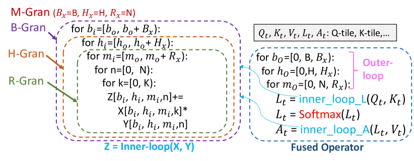
Fig. 6: For loop of fused L-Softmax-A (or shortened as L-A in the paper) and the choice of granularity.

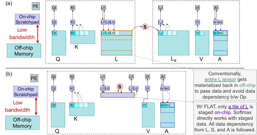
Fig. 7: (a) Baseline and (b) Flat dataflow. Flat performs inter-operator fusion of L, A while respecting data dependencies introduced by Softmax. Flat-tile enables staging slices of the logits tensor in the on-chip scratchpad increasing effective memory bandwidth. This fused, interleaved execution of L, A yields higher compute utilization and improved performance.

5 Flat Dataflow Implementation

To fuse two tensor operators $X$ and $Y$, we divide the loop nests into two groups: “outer-loop” and “inner-loop”. We use $L$ and $A$ for illustration as shown in  Fig. 6, but the principles are applicable to any set of consecutive tensor operators. The outer-loops are shared across L and A. The inner-loops are unique for each operator. After fusion, the fused operator has two inner-loops, which we run one after another (interleaved), and iterate through the shared outer-loop. Considerations for tile sizes to address the data dependence and on-chip memory constraints (§ 4.2) are discussed in this section.

5.1 Flat-tile and Execution Granularity

Flat employs two levels of tiling: intra-operator tiling and inter-operator tiling. We name each tile in inter-operator tiling, a Flat-tile. Flat computes Flat-tile activations from L and feeds it through Softmax and to A. Flat-tiles, the inner-loop in Fig. 6, essentially specifies how many slices of the partial intermediate tensor are calculated in one pass of the fused-operator in Fig. 7(b). The minimum granularity of the Flat-tile is determined by the data dependence constraint of Softmax and called row-granularity (discussed in § 5.2), for effectively collecting a group/tile of (input) data that fulfills the Many-to-Many dependency pattern of Softmax. We progressively build larger (coarser-grain) tiles, namely, tiling multiple number of rows at a time ($R_{x}$), multiple number of heads ($H_{x}$), and finally, multiple number of (micro-)batches ($B_{x}$) in the tile. We refer to these as Row (R-Gran), Head (H-Gran), and Batch (B-Gran) granularity respectively (discussed in § 5.3). Further, the most intuitive baseline of moving the entire intermediate tensor (namely the entire output of L) on-chip is referred to as Batch-Multi-Head granularity (M-Gran), as shown in Fig. 6.

5.2 Managing Constraints from Data Dependency

Basic execution unit $\rightarrow$ “Row-granularity”. The Softmax reduction is along the key dimension: this effectively captures the relative weight of each token in the query sequence against other tokens in the key sequence. The minimum Softmax execution requires an [1, N] input array, which in turn requires a query of [1, D] and a key of [D, N], as illustrated in Fig. 1 Step- and Step- . This forms our basic tiling unit (finest granularity)—row-granularity, which respects the data dependency introduced by the Softmax while keeping minimum number of elements to pass between L and A. Flat restricts the tile sizes to operate in multiples of this row-granularity.

5.3 Managing Constraints from On-Chip Memory

M-Gran, B-Gran, H-Gran: Leveraging Limited Reuse of f(L, A). Coarser granularities require staging larger tiles in the on-chip memory. As sequence lengths increase this can increase rapidly (recall the O($N^{2}$) growth). To fit into the limited on-chip memory, one may target finer granularities, e.g., moving from M-Gran to B-Gran (i.e., effectively tiling micro-batches). In general, while this helps reduce the size of the tile, when we are tiling two operators at finer granularity at the outer-loop, we may trade-off the reuse opportunity at the inner-loops. For example, for f(FC, FC) and f(CONV, CONV), when decreasing the batch size (i.e., micro-batching), we directly reduce the number of times a weight can be reused. The weights need to be re-fetched again and again for each micro-batch. This effect is exacerbated when considering finer granularities such as H-Gran for the weight-activation K/Q/V/O operators. The reduced reuse opportunity by inter-operator tiling reduces the achievable performance, even though the fused operator has large operational intensity (Fig. 5). In contrast, L and A are activation-activation operations (Fig. 2). Each new activation of L needs to compute with a new activation of A, i.e., there are no reuse opportunities at the algorithmic level. Decreasing the tiling granularity (M-Gran to B-Gran to H-Gran), does not preclude any reuse opportunity, since there are no reuse opportunities at the algorithmic level. Thus, the finer M-Gran, B-Gran, H-Gran in Flat are well-suited for f(L, A).

R-Gran: Extreme Large Sequence Range. To enable very long sequence lengths [46, 69, 14], but with limited on-chip memory resources [39, 88], we need to tile at even finer granularity, namely R-Gran. However, finer granularities come with an associated trade-off: when we reduce the number of rows ($R_{x}$), we will also reduce the reuse opportunity in the matrix multiplication itself. For example, even for L/A fusion, using fewer rows means the same key vectors need to be fetched multiple times across the interleaved cross-operator outer loops. Further, reducing number of rows at the outer-loop could also decrease the achievable performance at the inner-loop, e.g., not enough dimension size to fully utilize PE array. Thus, Flat co-explores inter-operator (optimizing the outer-loop) and intra-operator dataflow (optimizing the inner-loop) to mitigate these potential sources of inefficiencies.

On-chip buffer requirement. Table 1 lists the required on-chip buffer size using Flat. We derive the R-Gran value here (others follow similar reasoning). L operator consumes (Rd+Nd)x2 size of the on-chip buffer (2 to account for double buffering), and A consumes (Nd+Rd)x2. RN for buffering the intermediate tensor (Flat-tile) (no double buffering since it does not interact with off-chip memory), whose on-chip buffer requirement is shown in Table 1.

HW support to implement Flat. Flat requires minimal HW support: (1) controller to recognize the proposed fine-grained dataflow and (2) on-chip buffer to be software-addressable to support tiling. These features are supported by most recent industry and academic accelerators [39, 77, 3, 88].

Table 1: Buffer requirement for tiling granularity. M: batched Multi-head, B: Batch, H: Head, R: Row.

Granularity	M-Gran	B-Gran	H-Gran	R-Gran
Buffer Req.	$\mathcal{O}(8BDN+BHN^{2})$	$\mathcal{O}(8DN+HN^{2})$	$\mathcal{O}(8Nd+N^{2})$	$\mathcal{O}(4Rd+4Nd+RN)$

6 Evaluation Methodology

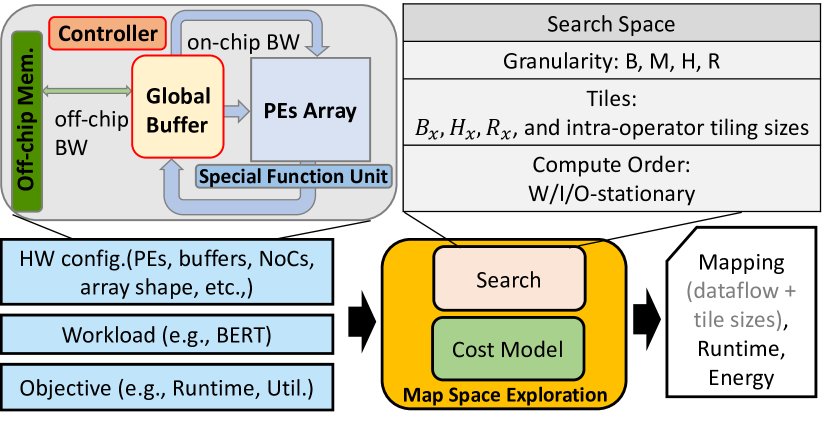
Fig. 8: Map space exploration framework. (Special Function Unit: for computing non-linear operations, e.g., softmax, activation.)

6.1 Accelerator Modeling Methodology

We developed a detailed analytical cost model to estimate the performance and energy consumption of Flat across a range of hardware accelerators configurations, following similar methodology as prior work [64, 50]. We meticulously model the major microarchitectural blocks commonly shared by most DNN accelerators as outlined in Figure 8. Based on this model, we collect the relevant architectural details, which later are used to compute the accelerator performance metrics.

Compute model. We model the compute array as a collection of processing elements with configurable bandwidth from/to the global on-chip buffers. The compute array model supports common intra-operator dataflow, including weight, input, and output stationary. In addition, we model various data distribution and reduction NoCs, including systolic, tree, or crossbar structures to study the the trade-offs between compute bandwidth and distribution-collection time [50, 51]. Following this methodology, we model TPU [40] (systolic-array) as well as other spatial array accceleraors, such as Eyeriss v2 [10] and MAERI [51]). We also carefully model the overhead of switching tiles for filling and draining data to reflect the cold start and tailing effect. Finally, we account for softmax operation runtime in all the evaluations.

Buffering model. Studying dataflow optimization techniques demand for a detailed modeling of buffers. To achieve this objective, we model PE arrays with local scratchpad for input, weight, intermediate results, and output storage. We add the on-chip global buffer to store the intra- and inter-operator tiles. The performance model also includes the data spilling overhead. That is when the live memory footprint (buffer requirement for staging data on-chip) is larger than the on-chip global buffer capacity.

Memory bandwidth. Since there are multiple microarchitectural units that access the on-chip and off-chip memories, we model them as limited bandwidth shared-hardware resources. That is, if the access rate to a shared memory resource exceeds a pre-defined bandwidth, the data accesses are throttled. This overhead manifests as longer runtime. A key feature of our simulation methodology is the detailed modeling of the accelerator memory hierarchy to systematically assess the memory-boundedness of attention operators and their pressure on off-chip memory bandwidth.

Energy model. Collecting the detailed activity counts from the analytical model, we use Accelergy [100] framework to estimate the energy consumption for the major microarchitectural blocks. That includes compute, on-chip memory, and off-chip memory communications. Note that Flat neither alters the total number of computations nor the total number of accesses to the on-chip global buffer. Instead, it optimizes the number of off-chip memory accesses, which is the major contributor to the overall accelerator energy consumption [83, 9].

Map-space exploration workflow. We also integrate a map-space exploration (MSE) workflow (Fig. 8) into our simulation framework. The main purpose of this exploration workflow is to carry out a search algorithm in a predefined map space governed by the cost model. In this work, we use exhaustive search to find the optimal design point uniformly across all the dataflow optimizations. MSE includes both intra- and inter-operator dataflow optimization space (enabling optimal dataflow comparisons with and without Flat technique later in Table 3 and § 7). The relevant architectural parameters for this optimization space are outlined in Fig. 8.

Comparison to prior accelerator modeling tools. There are several popular open-sourced DNN accelerator modeling frameworks [64, 50, 101, 18, 74, 59]. However, none of them offer support for cross-layer performance (and reuse) modeling, assuming layer-by-layer execution. In contrast, our framework evaluates the performance of DNN models in both single-layer and cross-layer manner, enabling various cross-operator fusion studies. To ensure the integrity and correctness of our framework, we compared the simulation results from our framework under single-layer modeling to MAESTRO [50]. The performance metrics are within $1\%$ difference to MAESTRO’s results.

Target accelerator configurations. We evaluate the benefits of Flat on two different accelerator regimes, namely cloud and edge accelerators. As outlined in Table 2, we set the accelerator configurations in our model following the designs proposed for cloud [39, 88] and edge [10, 76, 25] accelerators. In all the evaluations, we allot sufficient FLOPs to the Special Function Unit (Fig. 8) in order to eradicate the expected compute bottlenecks, uniformly across all the dataflow variants.

Evaluation metrics. For all the evaluations, we use performance and energy savings as efficiency metrics. For comparisons between different models, we normalize the runtime of each dataflow by the ideal runtime of the target workload as follows:

$$Util=\frac{\mathrm{Runtime}_{ideal}}{\mathrm{Runtime}_{dataflow}}$$

; where $\mathrm{Runtime}_{ideal}$ is the arithmetic optimal runtime of the current workload. That is, the total computes in a model divided by the peak FLOPs of the target accelerator. $\mathrm{Runtime}_{dataflow}$ represents the achieved runtime by a dataflow optimization. This normalized runtime metric explains how far the current dataflow is from its arithmetic optimum. This metric is an indication of the distance to the dataflow compute-boundray in the roofline model as well as compute resource utilization ($Util$).

Flat on GPUs. Some of our evaluations demonstrate the efficiency of FLAT on Nvidia-Tesla-T4 [87] GPU with 16GB memory. Since we could not modify the underlying highly-optimized CUDA APIs, we manually implemented the “einsum” operation as nested loops for baseline. We prototyped fused L-A by modifying this nested loop.

Workloads. We study a range of recent attention-based models, including BERT-Base [89] (BERT), TransformerXL [17] (TrXL), FlauBERT [53] (FlauBERT), T5 [70] (T5), and XLM-MLM-En [52] (XLM). We evaluate these models under different sequences lengths ranging from $N=512$ to $N=64K$ to imitate attention-based models with long sequence length [5, 46]. We also study a future-proofing sequence length of size $N=256K$. We use a batch size of 64 for all the models. Note that the batch size choice is immaterial to our dataflow optimization.

Table 2: The HW compute resource and BW configuration of Edge and Cloud platforms in the evaluation sections. The on-chip memory capacity is varied across explored design-points.

Platform	$\#$ of PEs	On-Chip BW	Off-Chip BW
Edge	32$\times$32	1 TB/Sec	50 GB/Sec
Cloud	256$\times$256	8 TB/Sec	400 GB/Sec

Table 3: Comparisons dataflow configurations.

Dataflow	Design Point	Description
Naïve (Intra-Operator)	Naïve	Intra-operator weight-stationary dataflow with fixed tile size, similar to [25, 20].
Flex (Intra-Operator)	Flex-Opt	We exhaustively search for optimal intra-operator dataflow, reflecting the optimal solution can be found in existing intra-operator mappers [62, 10, 41, 39].
Flat (Intra-/Inter-Operator)	Flat-Opt	We exhaustively search for optimal intra-operator as well as inter-operator dataflow.

Table 4: Run time performance improvement of Flat over Naïve and Flex, using sequence length=512 and Edge platform compute + BW configurations (Table 2) with varying on-chip buffer sizes (200K, 20M and 2GB). Flat shows its advantage when buffer sizes are limited.

Run time Improvement	L/A layer			End-to-End
	2G(B)	20M	200K	2G	20M	200K
Flat over Naïve	1.7$\times$	3.3$\times$	3.2$\times$	1.5$\times$	1.6$\times$	3.2$\times$
Flat over Flex	1.02$\times$	1.02$\times$	1.7$\times$	1.02$\times$	1.02$\times$	1.1$\times$

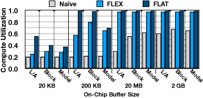
(a) Sequence Length = 512

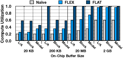
(b) Sequence Length = 4 K

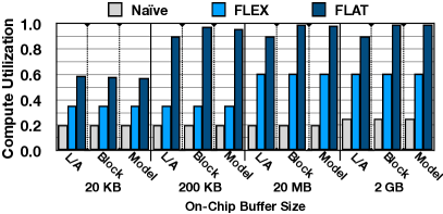
(c) Sequence Length = 64 K

Fig. 9: Comparisons of compute utilization of BERT under Edge platform w/ different input sequence lengths. We sweep the size of available on-chip buffer from 20KB to 2GB. The figures demonstrate three different performance analysis, (first bar) L-A $\rightarrow$ focusing on performance difference at the L, A operators; (second bar) Block $\rightarrow$ consider all operators in the attention block; and (third bar) Model $\rightarrow$ a model-wise (end-to-end) performance.

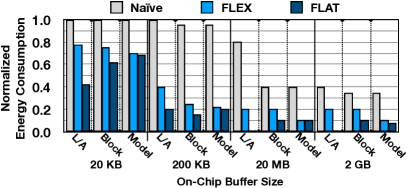
(a) Sequence Length = 512

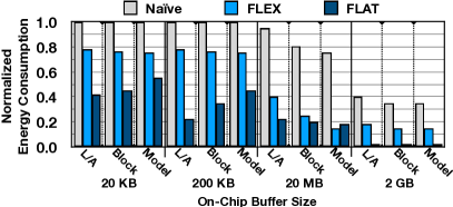
(b) Sequence Length = 4 K

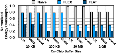
(c) Sequence Length = 64 K

Fig. 10: Comparisons of energy consumption of BERT under Edge platform with different input sequence length. We normalize the energy consumption results to the largest value in each sub-plot. Each bar represents the same analysis as described in Figure 9.

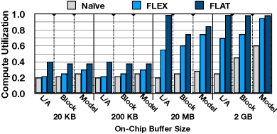
(a) Sequence Length = 512

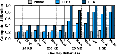
(b) Sequence Length = 4 K

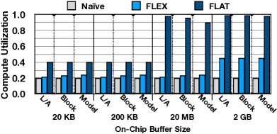
(c) Sequence Length = 64 K

Fig. 11: Comparisons of compute utilization of XLM under Cloud platform with different input sequence length. We sweep the size of available on-chip buffer from 20KB to 2GB. Each bar represents the same analysis as described in Figure 9.

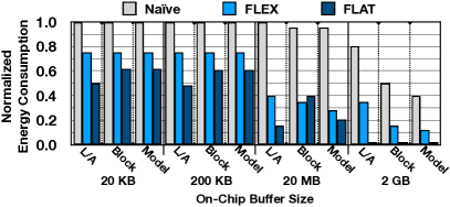
(a) Sequence Length = 512

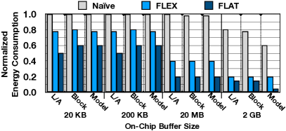
(b) Sequence Length = 4 K

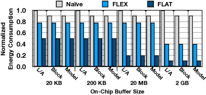
(c) Sequence Length = 64 K

Fig. 12: Comparisons of energy consumption of XLM under Cloud platform with different input sequence length. We normalize the energy consumption results to the largest value in each sub-plot. Each bar represents the same analysis as described in Figure 9.

7 Evaluation I: Flat Dataflow Efficacy

In this section, we fix the “headline” “HW resources” (i.e., FLOPs and off-chip memory bandwidth) as outlined in Table 2 and sweep-and-explore other microarchitectural parameters relevant to the dataflow efficiency, including on-chip memory size and dataflow variations (Naïve, Flex and Flat as explained in Table 3). The on-chip memory size assesses the dataflow optimizations associated to the large intermediate tensor size in the attention layers. The goal of this section is demonstrate the benefits of Flat across a range of hardware and dataflow configurations, without biasing to any specific design point.

Runtime performance. Table 4 shows the run time performance improvement of Flat (Flat-Opt) over Naïve (the baseline dataflow without any optimizations) and Flex (Flex-Opt), under commonly observed on-chip buffer sizes and sequence length (512-token). We observe 1) providing huge on-chip buffer resources (2GB), Flat with its fused operation and improved data-reuse can improves Naïve and Flex; 2) at limited buffer resources, Flat becomes handy owing to its reduced on-chip buffer footprint. For example, at 200KB, Flat-Opt improves the current state-of-the-art baseline – Flex-Opt – by 1.7$\times$ on the focusing L-A operations, which contributes to 1.1$\times$ improvement of end-to-end performance. Note that owing to the quadratic complexity of L-A operations, L-A operations will become more dominant at larger sequence length. For e.g., in this evaluation with 512-token, L-A operation contributes only 10$\%$ of the computes to the end-to-end model; however, it increases to 47$\%$ and 78$\%$ at 4K-token and 16K-token. Next, we show the efficacy of Flat under a sweep of buffer sizes, sequence length, and with perspectives of different granularity of the models (operations, layers, and end-to-end).

Sensitivity to sequence length. As described in § 6.1, we use $Util$, a normalized run time performance metric to show the performance difference of different sequence lengths, buffer size, and model granularity in the same plot. As 9a-LABEL:sub@fig:util_cpr_edge_c shows, Flat-Opt consistently outperforms Naïve and Flex-Opt. Analyzing the results indicate that though tensor-tensor fusion seems to be complicated and deemed as non-profitable, Flat can efficiently execute tensor-tensor fusion in attention layers and harvest the highest performance gains. In 9a-LABEL:sub@fig:util_cpr_edge_c, as the sequence length increases, the on-chip buffer requirement increases quickly (Table 1). Under this scenario, most of the accelerator design points in Flex design space starts to hit the memory boundedness. However, applying the Flat technique, we can effectively reduce the memory requirement and thus providing a better scalability to sequence length. At the optimal design point (Flat-Opt) reaches nearly 1.0 compute utilization with 10$\times$-100$\times$ less on-chip buffer requirement in Edge accelerator as shown in 9a-LABEL:sub@fig:util_cpr_edge_c, and 100$\times$-1000$\times$ in Cloud accelerator as shown in 11a-LABEL:sub@fig:util_cpr_cloud_c, a scarce and critical hardware resource for accelerators, compared to Flex-Opt.

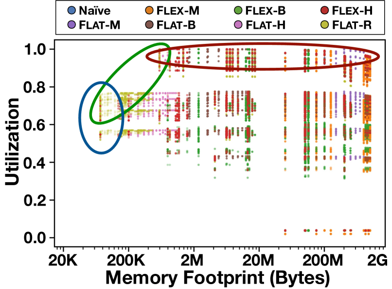
Fig. 13: The design space of Flat of BERT w/ input sequence length of 512 in Edge. Flex dataflow (Flex-X): Flex dataflow with X-granularity. Flat dataflow (Flat-X): Flex dataflow with X-granularity, where X could be M (batch-Multi-head), B (Batch), H (head), or R (row). The design-point with the highest utilization, given a buffer constraint represents Flex-Opt and Flat-Opt (Table 3). The highlighted regions represent: “Blue (bottom left)” $\rightarrow$ low memory footprint, “Green (top left)” $\rightarrow$ high utilization per memory footprint, and “Red (top)” $\rightarrow$ high utilization.

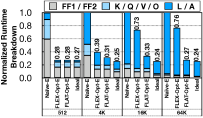
(a) BERT on Edge Accelerator

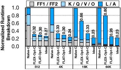
(b) XLM on Cloud Accelerator

Fig. 14: End-to-end latency breakdown. The suffix “E” and “C” indicate E(dge) and C(loud) platforms. Naïve, FLEX-Opt, and FLAT-Opt are defined in Table 3.

Table 5: The End-to-End speedup and energy-consumption ratio of Flat-Opt-E(dge) over Flex-Opt-E(dge) and Flat-Opt-C(loud) over Flex-Opt-C(loud) on different models.

Flat-Opt-Edge vs. Flex-Opt-Edge
Edge	Geomean Speadup = 1.75$\times$					Geomean Consumption Ratio = 0.56$\times$
Seq. Length	512	4K	16K	64K	256K	512	4K	16K	64K	256K
BERT	1.02	1.27	2.21	2.84	3.10	0.98	0.78	0.44	0.34	0.31
TrXL	1.02	1.23	2.06	2.75	3.07	0.98	0.81	0.48	0.35	0.31
FlauBERT	1.01	1.11	1.62	2.26	2.67	1.00	0.90	0.61	0.43	0.36
T5	1.03	1.34	2.40	2.93	3.13	0.97	0.74	0.41	0.33	0.31
XLM	1.00	1.05	1.35	1.87	2.38	1.00	0.95	0.74	0.52	0.31
Average	1.02	1.20	1.89	2.50	2.85	0.99	0.83	0.52	0.39	0.32
Flat-Opt-Cloud vs. Flex-Opt-Cloud
Cloud	Geomean Speedup = 1.65$\times$					Geomean Energy Consumption Ratio = 0.45$\times$
Seq. Length	512	4K	16K	64K	256K	512	4K	16K	64K	256K
BERT	1.16	1.38	1.46	2.23	2.72	0.71	0.68	0.11	0.34	0.27
TrXL	1.13	1.34	1.45	2.20	2.71	0.73	0.27	0.13	0.35	0.27
FlauBERT	1.07	1.21	1.42	2.21	2.93	0.87	0.80	0.72	0.49	0.37
T5	1.18	1.43	1.48	2.26	2.73	0.69	0.66	0.50	0.33	0.27
XLM	1.02	1.06	1.13	1.98	3.09	0.97	0.89	0.78	0.50	0.31
Average	1.11	1.28	1.38	2.17	2.83	0.79	0.61	0.33	0.40	0.30

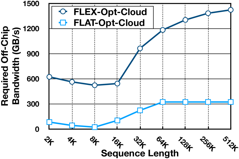
Fig. 15: The required off-chip bandwidth to reach a compute utilization rate higher than 0.95 in the most BW-intensive L-A operator when running XLM.

Sensitivity to end-to-end performance. So far, we analyze the performance for only L and A operators, while not considering other operators within the model. As shown in the first row of Fig. 9 from left to right, we observe that the effect of L/A operators are diluted as more operators are considered. In attention-based models, FC/GEMM and attention operators, namely L and A, are generally the most dominant computation. For FC/GEMM, the typical single (intra-)operator dataflow is often sufficient to reach a high compute utilization, and hence Flat-Opt and Flex-Opt performs equally well for these operators. As we can see, for the sequence length below 512, both Block-level and Model-level (i.e., End-to-End) performance is dominated by FC/GEMM operators. Therefore, the gains from Flex-Opt and Flat-Opt are immaterial. The significant gains from our approach emerge when the sequence length increases beyond 512 to 4K, 16K, and to 64K. Under these long-sequence lengths, the runtime contribution of L and A operators grows from 12$\%$ to 49$\%$, 79$\%$, and 94$\%$, respectively. This increase causes our proposed Flat-Opt to outperform Flex-Opt significantly even in Block and Model level scenarios.

Energy consumption. 10a-LABEL:sub@fig:util_cpr_edge_f and 12a-LABEL:sub@fig:util_cpr_cloud_f show the energy consumption for BERT on Edge platform and XLM on Cloud platform, respectively. It is worth to mention that high utilization does not directly translate to better energy savings; however, highly correlated. Data points with high compute utilization generally employ better memory access patterns (e.g., less off-chip memory access and better data reuse) and thus impose less cost in terms of memory access energy, the dominant contributor to the overall energy consumption of DNN accelerators. We observe that Flat-Opt reduces the energy consumption by around 1.5$\times$-2.0$\times$ comparing to Flex-Opt.

Map space exploration. Fig. 13 shows a holistic view of the entire design space of Flat dataflow. The top-left corner of the diagram indicates high utilization with the least memory footprint. For each dataflow, there are abundance of parameters that can be tuned under different optimization objectives and design constraints. For example, while in this work, we focus on maximizing the compute utilization, one may choose other objectives such as maximizing utilization normalized to memory footprint size, leading to points in the top-left corner, or the least memory footprint size, leading to points in the left-most region. From Fig. 13, we can see that different dataflow configurations in the design space indeed represent notable differences in performance and memory requirement. This highlights the impact and importance of the design choices and dataflow optimizations.

Case study on protein sequencing. Long sentence protein sequencing can model protein interaction networks without the large sequence alignments [14]. We follow the same methodology as in Performer [14] on the TrEMBL protein sequencing dataset [15] on a target accelerator with 16GB memory (§ 6.1). We show the memory requirement when the number of attention blocks varies with the sequence lengths of 8K (Table 6) and 16K (Table 7). In both cases, FLAT unlocks the opportunity to use larger transformer models (Table 6) and/or larger sequence length (Table 7), potentially increasing model performance. In summary, Flat outperforms recent DNN dataflow approaches [32, 41, 50, 64, 35, 11, 39, 62, 20] on attention models owing to its specialized fusion and tiling tailored for attentions, enabling longer sequence lengths.

8 Evaluation II: Accelerator Comparison

In this section, we contrast the performance of specific accelerator design points with and without the Flat dataflow.

8.1 Cloud and Edge Accelerators

Table 6: Flat on the TrEMBL protein sequencing dataset [15] on a target accelerator (Tesla T4 GPU [87]) with 16GB memory, using sequence length = 8K.

Memory Req.(GB)	Number of Attention Blocks (Sequence Length=8K)
	1	2	3	4	5	6
Baseline	4.6	9.1	13.7	18.2 -OOM	22.2 -OOM	27.3 -OOM
Flat	0.9	1.8	2.7	3.5	4.4	5.3

We start by selecting two specific hardware design points, namely a Cloud and an Edge accelerator, with headline HW resources that closely resemble a TPU-v3 [39] and Edge TPU [25, 76], as shown in Table 2. We fix the on-chip buffer capacity to 512KB [25] and 32MB [39] for Edge and Cloud accelerators, respectively. Analyzing these accelerators across different dataflow spaces (Table 3), namely Naïve, Flex, and Flat, forms a concrete and reasonably realistic accelerator design space. Similar to previous sections, we name the optimal accelerator design point in each design space: Naïve Edge, Flex-Opt-Edge, and Flat-Opt-Edge for edge accelerator, and Naïve-Cloud, Flex-Opt-Cloud, and Flat-Opt-Cloud for cloud accelerator, respectively.

Table 7: Flat on the TrEMBL protein sequencing dataset [15] on a target accelerator (Tesla T4 GPU [87]) with 16GB memory, using sequence length = 16K.

Memory Req.(GB)	Number of Attention Blocks (Sequence Length=16K)
	1	2	3	4	5	6
Baseline	17.5 -OOM	35 -OOM	52.5 -OOM	70.0 -OOM	87.5 -OOM	105.0 -OOM
Flat	2.8	5.6	8.5	11.3	14.1	16.9 -OOM

Accelerator performance. As show in 14a, Flex-Opt-Edge and Flat-Opt-Edge share the same normalized runtime for K/Q/V/O and FF1/FF2. This similarity in performance is because in Flat-Opt-Edge, both K/Q/V/O and FF1/FF2 are treated as non-fused operators, and hence the map space for them are the same as the one in Flex-Opt-Edge. In edge accelerator, when the sequence length is 512, Flat-Opt-Edge and Flex-Opt-Edge both reach a near optimal performance. However, when the sequence length increases to 4K, 16K, and 64K, the performance gap between Flat-Opt-Edge and Flex-Opt-Edge widen. For example, at sequence length of 64K, Flat-Opt-Edge runs 2.8$\times$ faster than Flex-Opt-Edge, showing the efficiency of our dataflow optimization. In the cloud accelerator (Fig. 14(b)), the performance difference between Flat-Opt-Cloud and Flex-Opt-Cloud exaggerates even further. For example, at sequence length of 64K, Flat-Opt-Cloud runs 3.07$\times$ faster than Flex-Opt-Cloud. That is partly because of the larger model size for the cloud accelerator that enables Flat-Opt-Cloud to better utilize the on-chip hardware resources.

Comparisons across different models. Table 5 compares the performance of different dataflow optimizations across various transformer models. Compared to Flex-Opt-Edge, Flat-Opt-Edge delivers 1.75$\times$ speedup in edge accelerator, while significantly reducing the energy consumption by 44$\%$. In cloud accelerator, Flat-Opt-Cloud achieves 1.65$\times$ speedup and 55$\%$ energy savings over Flex-Opt-Cloud. These results show the broad application of Flat in improving the performance of various attention-based models under different design constraints.

Memory bandwidth requirement. Effectively using a limited off-chip bandwidth is an critical factor in the scalability of the hardware accelerator. That is because most DNN operations are often memory-bound and the off-chip memory bandwidth is often shared across different microarchitectural components in the system. In Fig. 15, we show the peak off-chip bandwidth requirement to achieve a compute utilization over 0.95 for L and A attention operators. The left hand side of the U-shape of Fig. 15 comes from the increase in the operational intensity and thus decrease of the bandwidth-boundedness as sequence length increases (§ 3.1).

The right hand side of the U-shape of Fig. 15 is caused by the quadratic and linear increase of on-chip memory requirement as sequence length increases for Flex and Flat, respectively. On average, Flat-Opt-Cloud reduces the off-chip bandwidth requirement by 82$\%$ against Flex-Opt-Cloud. Similarly, when evaluated under the edge scenario running BERT, Flat-Opt-Edge achieves 71$\%$ reduction, on average, in the off-chip bandwidth requirement against Flex-Opt-Edge. In summary, we demonstrate that Flat with its advantage of lowering on-chip buffer footprint can improve attention performance under existing Edge [25] and Cloud [39] DNN accelerators.

8.2 Flat Compatibility with other Accelerators

Flat compatibility on GPU. We implement and evaluate Flat on Nvidia-Tesla-T4 [87] with 16GB memory (§ 6.1). We use the BERT-Edge model and perform two experiments: (1) We fix the sequence length to 256 and sweep the batch size (Table 8), and (2) we fix the batch size to one and sweep the sequence length (Table 9). Table 8 shows that FLAT can run faster than baseline and supports larger batch sizes, whereas Table 9 demonstrates that FLAT runs faster than baseline and supports up to 64K-word under the GPU-device we use.

Table 8: Runtime improvement of attention layer on Tesla-T4 [87] GPU under different batch sizes.

Runtime (ms)	Batch Size (Sequence Length=256)
	1	16	64	128	256	1K	2K
Baseline	36	630	2,520	5,230	OOM	OOM	OOM
FLAT	28	480	1,870	3,740	7,560	34,010	OOM

Table 9: Runtime improvement of attention layer on Tesla-T4 [87] GPU under different sequence length.

Runtime (ms)	Sequence Length (Batch Size=1)
	128	512	2K	4K	16K	64K	128K
Baseline	12	74	697	OOM	OOM	OOM	OOM
FLAT	11	43	175	424	4,599	64,350	OOM

Flat compatibility with sparse-attention accelerators. Recent sparse-attention accelerators such as ELSA [30] and Sanger [57] eschew model accuracy for improved performance. Whereas Flat is a software-only method with no repercussions for model accuracy, which can readily be adapted across various platforms (e.g. Edge or Cloud). ELSA implicitly supports and implements a limited form of inter-layer fusion operation at row granularity in hardware. Sanger, a sparse-attention accelerator with a systolic array core, also employs one narrow form of fusion per row of PEs. Both fusions are similar to one of many supported fusion granularity in Flat (§ 5.2). In particular, Flat selects the proper granularity level (e.g. row, head, and batch as described in § 5.1) according to on-chip memory resources. To quantitatively evaluate the impact of sparsity on Flat, we extended our methodology (§ 6.1) to measure the memory-boundedness of L-A operators when L and A are sparse. We randomly sparsify L-A matrix with pruning ratio 50$\%$ in BERT and XLM on TPU-v3 platform resources [39]. The results (Fig. 16) emphasize that even with a high degree of sparsity, these operations are still memory-bound, which warrants the benefits of Flat.

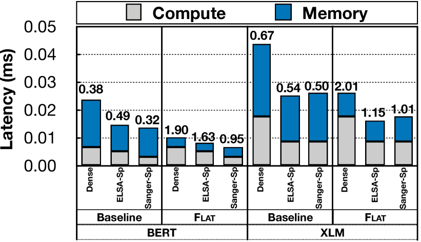
Fig. 16: The compute and memory time of L-A operations in BERT and XLM model under TPU-v3 configurations [39]. The valu on top of each bar indicates Compute-/Memory-time ratio. Compute-/Memory-time ratio (C/M) < 1 means memory-boundedness; Likewise, C/M > 1 means compute-boundedness, and the dataflow/system has more flexibility to operate to fully utilize the compute resources. We compare dense attention (Dense), ELSA-style sparse attention (ELSA-sp) [30], Sanger-style sparse attention (Sanger-sp) [57] with and without Flat optimization. It shows that both ELSA [30] and Sanger [57] can effectively improve the attention performance, and both ELSA and Sanger can leverage Flat to reduce the memory-boundedness (note that C/M increases to near or above 1.0 after applying Flat) and further improve the performance.

9 Related Works

Dataflow and mapping. Most work on DNN hardware dataflow techniques focus on individual CONV [62, 20, 9, 41, 64, 77, 58, 37, 101, 18, 24, 23, 90, 105, 91, 80, 103], GEMM [40, 97, 49] operators, or loop reordering for transformer operations [68]. Some recent works consider fusion of multiple CONV operator [2, 96]. Andrei et al. [36] merely targets operation fusion between MatMul operators and element-wise operators. Fusing multiple heads of the attention operators [63, 60] primarily involves adding an additional loop over the H independent heads, which is already captured by Flex. They, however, do not explore dependent MatMul-Softmax-MatMul fusion, which is more complicated. Flat targets such fusion and enables significantly higher performance.

Algorithmic optimization. Techniques such as quantization [78, 44, 104, 107], pruning [92, 55, 102, 28, 95, 73], and distillation [75, 38, 82, 94] are used for compressing Attention-based models. There are a large body of algorithmic changes to attention mechanism [79, 65, 67, 12, 5], learned sparsity [16, 46, 72, 85] low-rank and kernel methods [93, 42, 13, 14], and others [17, 5, 69]. These techniques impact model quality and are orthogonal to the ideas developed in this paper. Flat can be leveraged in association with these techniques when deployed on DNN accelerators to further improve run time and energy.

Matrix-Matrix fusion accelerators. The core of Graph Neural Networks (GNNs) includes two consecutive matrix computations (“aggregate” and “combine”). GCNAX [54] and GRIP [45] form a matrix-matrix loop fusion dataflow to optimize the throughput and energy efficiency. There are different challenge and focus for matrix-matrix fusion in GNNs and attentions. 1) The dataflows of GNN accelerators [54, 45] optimize matrix-matrix fusion (Fig. 3(c)-left column), whereas the dataflows of attention optimizes matrix-Softmax-matrix fusion (Fig. 3(c)-right column). 2) GNN includes one activation-weight and one activation-activation matrix computation, whereas attention has both matrix computations as activation-activation. 3) The key challenge of GNN is the sparsity in the “aggreate” matrix, whereas attention is challenged by the quadratic complexity of intermediate activation matrix between two matrix-multiplies.

Attention accelerators. $A^{3}$ [29] and ELSA [30] propose dedicated attention accelerators and leverage approximate computation to accelerate attention layers. Sanger [57] uses quantized query and key to predict attention matrix and rearranges the sparse attention matrix for better utilization. These technique trade-off performance with model quality. Flat, by contrast, does not impact model quality, and is a generic yet efficient dataflow technique that can be leveraged on most existing accelerators. SM6 [84] is an attention accelerator for RNN-based networks, which exposes different challenge and is orthogonal to this work.

Compiler optimizations. Fusion is a classic compiler technique [98, 1, 22, 19, 43, 8, 4, 47, 26]. However, ML compilers employ fusion in a limited fashion to fuse matrix operators with element-wise operators [61].

10 Conclusion

We identify that running attention-based models with long sequences is challenging because of low reuse in certain attention operators and quadratic growth of intermediate memory footprint, both of which compound memory bandwidth requirements. We propose Flat, a novel dataflow for attention layers employing inter-operator fusion (the first work to investigate this for attention layers), interleaved execution, and efficient tiling to enhance the operational intensity and provide high compute utilization, reduced off-chip bandwidth requirements and scalability to long sequence lengths.

References

- [1] Randy Allen and Ken Kennedy. Vector Register Allocation. IEEE Computer Architecture Letters, 1992.
- [2] Manoj Alwani, Han Chen, Michael Ferdman, and Peter Milder. Fused-layer CNN Accelerators. In MICRO, 2016.
- [3] Eunjin Baek, Dongup Kwon, and Jangwoo Kim. A Multi-Neural Network Acceleration Architecture. In ISCA, 2020.
- [4] Riyadh Baghdadi, Jessica Ray, Malek Ben Romdhane, Emanuele Del Sozzo, Abdurrahman Akkas, Yunming Zhang, Patricia Suriana, Shoaib Kamil, and Saman Amarasinghe. Tiramisu: A Polyhedral Compiler for Expressing Fast and Portable Code. In CGO, 2019.
- [5] Iz Beltagy, Matthew E Peters, and Arman Cohan. Longformer: The Long-document Transformer. arXiv preprint arXiv:2004.05150, 2020.
- [6] Prarthana Bhattacharyya, Chengjie Huang, and Krzysztof Czarnecki. Self-attention based context-aware 3d object detection. arXiv preprint arXiv:2101.02672, 2021.
- [7] Mark Chen, Alec Radford, Rewon Child, Jeffrey Wu, Heewoo Jun, David Luan, and Ilya Sutskever. Generative Pretraining from Pixels. In ICML, 2020.
- [8] Tianqi Chen, Lianmin Zheng, Eddie Yan, Ziheng Jiang, Thierry Moreau, Luis Ceze, Carlos Guestrin, and Arvind Krishnamurthy. Learning to Optimize Tensor Programs. In NeurIPS, 2018.
- [9] Yu-Hsin Chen et al. Eyeriss: An Energy-efficient Reconfigurable Accelerator for Deep Convolutional Neural Networks. JSSC, 2016.
- [10] Yu-Hsin Chen, Tien-Ju Yang, Joel Emer, and Vivienne Sze. Eyeriss v2: A Flexible Accelerator for Emerging Deep Neural Networks on Mobile Devices. JSSC, 2019.
- [11] Chen, Yu-Hsin and Krishna, Tushar and Emer, Joel and Sze, Vivienne. Eyeriss: An Energy-Efficient Reconfigurable Accelerator for Deep Convolutional Neural Networks. In ISSCC, 2016.
- [12] Rewon Child, Scott Gray, Alec Radford, and Ilya Sutskever. Generating Long Sequences with Sparse Transformers. arXiv preprint arXiv:1904.10509, 2019.
- [13] Krzysztof Choromanski, Valerii Likhosherstov, David Dohan, Xingyou Song, Jared Davis, Tamas Sarlos, David Belanger, Lucy Colwell, and Adrian Weller. Masked Language Modeling for Proteins via Linearly Scalable Long-context Transformers. arXiv preprint arXiv:2006.03555, 2020.
- [14] Krzysztof Choromanski, Valerii Likhosherstov, David Dohan, Xingyou Song, Andreea Gane, Tamas Sarlos, Peter Hawkins, Jared Davis, Afroz Mohiuddin, Lukasz Kaiser, David Belanger, Lucy Colwell, and Adrian Weller. Rethinking Attention with Performers. arXiv preprint arXiv:2009.14794, 2020.
- [15] UniProt Consortium. UniProt: A Worldwide Hub of Protein Knowledge. Nucleic Acids Research, 2019.
- [16] Gonçalo M Correia, Vlad Niculae, and André FT Martins. Adaptively Sparse Transformers. arXiv preprint arXiv:1909.00015, 2019.
- [17] Zihang Dai, Zhilin Yang, Yiming Yang, Jaime Carbonell, Quoc V Le, and Ruslan Salakhutdinov. Transformer-XL: Attentive Language Models Beyond a Fixed-Length Context. arXiv preprint arXiv:1901.02860, 2019.
- [18] Shail Dave, Youngbin Kim, Sasikanth Avancha, Kyoungwoo Lee, and Aviral Shrivastava. dMazeRunner: Executing Perfectly Nested Loops on Dataflow Accelerators. TECS, 2019.
- [19] Chen Ding and Ken Kennedy. Improving Effective Bandwidth Through Compiler Enhancement of Global Cache Reuse. Journal of Parallel and Distributed Computing, 2004.
- [20] Zidong Du, Robert Fasthuber, Tianshi Chen, Paolo Ienne, Ling Li, Tao Luo, Xiaobing Feng, Yunji Chen, and Olivier Temam. ShiDianNao: Shifting Vision Processing Closer to the Sensor. In ISCA, 2015.
- [21] Patrick Esser, Robin Rombach, and Björn Ommer. Taming Transformers for High-Resolution Image Synthesis. arXiv preprint arXiv:2012.09841, 2020.
- [22] Guang Gao, Russ Olsen, Vivek Sarkar, and Radhika Thekkath. Collective Loop Fusion for Array Contraction. In International Workshop on Languages and Compilers for Parallel Computing, 1992.
- [23] Mingyu Gao, Jing Pu, Xuan Yang, Mark Horowitz, and Christos Kozyrakis. TETRIS: Scalable and Efficient Neural Network Acceleration with 3D Memory. In ASPLOS, 2017.
- [24] Mingyu Gao, Xuan Yang, Jing Pu, Mark Horowitz, and Christos Kozyrakis. TANGRAM: Optimized Coarse-Grained Dataflow for Scalable NN Accelerators. In ASPLOS, pages 807–820, 2019.
- [25] Google. Coral AI. https://coral.ai/, 2020.
- [26] Google. TensorFlow XLA. https://www.tensorflow.org/xla, 2021.
- [27] Ben Graham, Alaaeldin El-Nouby, Hugo Touvron, Pierre Stock, Armand Joulin, Hervé Jégou, and Matthijs Douze. LeViT: a Vision Transformer in ConvNet’s Clothing for Faster Inference. In ICCV, 2021.
- [28] Fu-Ming Guo, Sijia Liu, Finlay S Mungall, Xue Lin, and Yanzhi Wang. Reweighted Proximal Pruning for Large-scale Language Representation. arXiv preprint arXiv:1909.12486, 2019.
- [29] Tae Jun Ham, Sung Jun Jung, Seonghak Kim, Young H Oh, Yeonhong Park, Yoonho Song, Jung-Hun Park, Sanghee Lee, Kyoung Park, Jae W Lee, et al. A^3: Accelerating Attention Mechanisms in Neural Networks with Approximation. In HPCA, 2020.
- [30] Tae Jun Ham, Yejin Lee, Seong Hoon Seo, Soosung Kim, Hyunji Choi, Sung Jun Jung, and Jae W Lee. ELSA: Hardware-Software Co-design for Efficient, Lightweight Self-Attention Mechanism in Neural Networks. In ISCA, 2021.
- [31] Kaiming He, Xiangyu Zhang, Shaoqing Ren, and Jian Sun. Deep Residual Learning for Image Recognition. In CVPR, 2016.
- [32] Kartik Hegde, Po-An Tsai, Sitao Huang, Vikas Chandra, Angshuman Parashar, and Christopher W Fletcher. Mind Mappings: Enabling Efficient Algorithm-Accelerator Mapping Space Search Extended Abstract. In ASPLOS, 2021.
- [33] Wen-Yi Hsiao, Jen-Yu Liu, Yin-Cheng Yeh, and Yi-Hsuan Yang. Compound Word Transformer: Learning to Compose Full-Song Music over Dynamic Directed Hypergraphs. arXiv preprint arXiv:2101.02402, 2021.
- [34] Cheng-Zhi Anna Huang, Ashish Vaswani, Jakob Uszkoreit, Ian Simon, Curtis Hawthorne, Noam Shazeer, Andrew M Dai, Matthew D Hoffman, Monica Dinculescu, and Douglas Eck. Music Transformer: Generating Music with Long-Term Structure. In ICLR, 2018.
- [35] Qijing Huang, Minwoo Kang, Grace Dinh, Thomas Norell, Aravind Kalaiah, James Demmel, John Wawrzynek, and Yakun Sophia Shao. CoSA: Scheduling by Constrained Optimization for Spatial Accelerators. arXiv preprint arXiv:2105.01898, 2021.
- [36] Andrei Ivanov, Nikoli Dryden, Tal Ben-Nun, Shigang Li, and Torsten Hoefler. Data Movement Is All You Need: A Case Study on Optimizing Transformers. In MLSys, 2021.
- [37] Zhihao Jia, Matei Zaharia, and Alex Aiken. Beyond Data and Model Parallelism for Deep Neural Networks. arXiv preprint arXiv:1807.05358, 2018.
- [38] Xiaoqi Jiao, Yichun Yin, Lifeng Shang, Xin Jiang, Xiao Chen, Linlin Li, Fang Wang, and Qun Liu. TinyBERT: Distilling BERT for Natural Language Understanding. arXiv preprint arXiv:1909.10351, 2019.
- [39] Norman P Jouppi, Doe Hyun Yoon, George Kurian, Sheng Li, Nishant Patil, James Laudon, Cliff Young, and David Patterson. A Domain-Specific Supercomputer for Training Deep Neural Networks. Communications of the ACM, 2020.
- [40] Norman P Jouppi, Cliff Young, Nishant Patil, David Patterson, Gaurav Agrawal, Raminder Bajwa, Sarah Bates, Suresh Bhatia, Nan Boden, Al Borchers, et al. In-Datacenter Performance Analysis of a Tensor Processing Unit. In ISCA, 2017.
- [41] Sheng-Chun Kao and Tushar Krishna. GAMMA: Automating the HW Mapping of DNN Models on Accelerators via Genetic Algorithm. In ICCAD, 2020.
- [42] Angelos Katharopoulos, Apoorv Vyas, Nikolaos Pappas, and François Fleuret. Transformers are RNNs: Fast Autoregressive Transformers with Linear Attention. In ICML, 2020.
- [43] Ken Kennedy and Kathryn S McKinley. Maximizing Loop Parallelism and Improving Data Locality via Loop Fusion and Distribution. In International Workshop on Languages and Compilers for Parallel Computing, 1993.
- [44] Sehoon Kim, Amir Gholami, Zhewei Yao, Michael W Mahoney, and Kurt Keutzer. I-BERT: Integer-only BERT Quantization. arXiv preprint arXiv:2101.01321, 2021.
- [45] Kevin Kiningham, Christopher Re, and Philip Levis. GRIP: A Graph Neural Network Accelerator Architecture. arXiv preprint arXiv:2007.13828, 2020.
- [46] Nikita Kitaev, Łukasz Kaiser, and Anselm Levskaya. Reformer: The Efficient Transformer. arXiv preprint arXiv:2001.04451, 2020.
- [47] Fredrik Kjolstad, Shoaib Kamil, Stephen Chou, David Lugato, and Saman Amarasinghe. The Tensor Algebra Compiler. In OOPSLA, 2017.
- [48] Tushar Krishna, Hyoukjun Kwon, Angshuman Parashar, Michael Pellauer, and Ananda Samajdar. Data Orchestration in Deep Learning Accelerators. Synthesis Lectures on Computer Architecture. Morgan & Claypool Publishers, 2020.
- [49] Aviral Kumar, Amir Yazdanbakhsh, Milad Hashemi, Kevin Swersky, and Sergey Levine. Data-Driven Offline Optimization for Architecting Hardware Accelerators. In ICLR, 2022.
- [50] Hyoukjun Kwon, Prasanth Chatarasi, Michael Pellauer, Angshuman Parashar, Vivek Sarkar, and Tushar Krishna. Understanding Reuse, Performance, and Hardware Cost of DNN Dataflow: A Data-Centric Approach. In MICRO, 2019.
- [51] Hyoukjun Kwon, Ananda Samajdar, and Tushar Krishna. MAERI: Enabling Flexible Dataflow Mapping over DNN Accelerators via Reconfigurable Interconnects. In ASPLOS, 2018.
- [52] Guillaume Lample and Alexis Conneau. Cross-Lingual Language Model Pretraining. arXiv preprint arXiv:1901.07291, 2019.
- [53] Hang Le, Loïc Vial, Jibril Frej, Vincent Segonne, Maximin Coavoux, Benjamin Lecouteux, Alexandre Allauzen, Benoît Crabbé, Laurent Besacier, and Didier Schwab. Flaubert: Unsupervised Language Model Pre-training for French. arXiv preprint arXiv:1912.05372, 2019.
- [54] Jiajun Li, Ahmed Louri, Avinash Karanth, and Razvan Bunescu. GCNAX: A Flexible and Energy-Efficient Accelerator for Graph Convolutional Neural Networks. In HPCA, 2021.
- [55] Zheng Li, Soroush Ghodrati, Amir Yazdanbakhsh, Hadi Esmaeilzadeh, and Mingu Kang. Accelerating Attention through Gradient-Based Learned Runtime Pruning. In ISCA, 2022.
- [56] Peter J Liu, Mohammad Saleh, Etienne Pot, Ben Goodrich, Ryan Sepassi, Lukasz Kaiser, and Noam Shazeer. Generating Wikipedia by Summarizing Long Sequences. arXiv preprint arXiv:1801.10198, 2018.
- [57] Liqiang Lu, Yicheng Jin, Hangrui Bi, Zizhang Luo, Peng Li, Tao Wang, and Yun Liang. Sanger: A Co-Design Framework for Enabling Sparse Attention using Reconfigurable Architecture. In MICRO, 2021.
- [58] Wenyan Lu et al. FlexFlow: A Flexible Dataflow Accelerator Architecture for Convolutional Neural Networks. In HPCA, 2017.
- [59] Linyan Mei, Pouya Houshmand, Vikram Jain, Sebastian Giraldo, and Marian Verhelst. ZigZag: A Memory-Centric Rapid DNN Accelerator Design Space Exploration Framework. arXiv preprint arXiv:2007.11360, 2020.
- [60] Vinh Nguyen, Sukru Burc Eryilmax, Karthik Mandakolathur, and Shar Narasimhan. Boosting NVIDIA MLPerf Training v1.1 Performance with Full Stack Optimization. https://tinyurl.com/3dku474c, 2021.
- [61] Wei Niu, Jiexiong Guan, Yanzhi Wang, Gagan Agrawal, and Bin Ren. DNNFusion: Accelerating Deep Neural Networks Execution with Advanced Operator Fusion. In PLDI, 2021.
- [62] Nvidia. NVDLA Deep Learning Accelerator. http://nvdla.org, 2017.
- [63] Nvidia. FasterTransforemr. https://github.com/NVIDIA/FasterTransformer, 2021.
- [64] Angshuman Parashar, Priyanka Raina, Yakun Sophia Shao, Yu-Hsin Chen, Victor A Ying, Anurag Mukkara, Rangharajan Venkatesan, Brucek Khailany, Stephen W Keckler, and Joel Emer. Timeloop: A Systematic Approach to DNN Accelerator Evaluation. In ISPASS, 2019.
- [65] Niki Parmar, Ashish Vaswani, Jakob Uszkoreit, Lukasz Kaiser, Noam Shazeer, Alexander Ku, and Dustin Tran. Image Transformer. In ICML, 2018.
- [66] Eric Qin, Ananda Samajdar, Hyoukjun Kwon, Vineet Nadella, Sudarshan Srinivasan, Dipankar Das, Bharat Kaul, and Tushar Krishna. SIGMA: A Sparse and Irregular GEMM Accelerator with Flexible Interconnects for DNN Training. In HPCA, 2020.
- [67] Jiezhong Qiu, Hao Ma, Omer Levy, Scott Wen-tau Yih, Sinong Wang, and Jie Tang. Blockwise Self-Attention for Long Document Understanding. arXiv preprint arXiv:1911.02972, 2019.
- [68] Markus N. Rabe and Charles Staats. Self-attention Does Not Need Memory. arXiv preprint arXiv:2112.05682, 2021.
- [69] Jack W Rae, Anna Potapenko, Siddhant M Jayakumar, and Timothy P Lillicrap. Compressive Transformers for Long-Range Sequence Modelling. arXiv preprint arXiv:1911.05507, 2019.
- [70] Colin Raffel, Noam Shazeer, Adam Roberts, Katherine Lee, Sharan Narang, Michael Matena, Yanqi Zhou, Wei Li, and Peter J Liu. Exploring the Limits of Transfer Learning with a Unified Text-to-Text Transformer. arXiv preprint arXiv:1910.10683, 2019.
- [71] Jonathan Ragan-Kelley, Connelly Barnes, Andrew Adams, Sylvain Paris, Frédo Durand, and Saman Amarasinghe. Halide: A Language and Compiler for Optimizing Parallelism, Locality, and Recomputation in Image Processing Pipelines. In PLDI, 2013.
- [72] Aurko Roy, Mohammad Saffar, Ashish Vaswani, and David Grangier. Efficient Content-Based Sparse Attention with Routing Transformers. Transactions of the Association for Computational Linguistics, 2021.
- [73] Hassan Sajjad, Fahim Dalvi, Nadir Durrani, and Preslav Nakov. Poor Man’s BERT: Smaller and Faster Transformer Models. arXiv preprint arXiv:2004.03844, 2020.
- [74] Ananda Samajdar, Yuhao Zhu, Paul Whatmough, Matthew Mattina, and Tushar Krishna. SCALE-Sim: Systolic CNN Accelerator Simulator. arXiv preprint arXiv:1811.02883, 2018.
- [75] Victor Sanh, Lysandre Debut, Julien Chaumond, and Thomas Wolf. DistilBERT, A Distilled Version of BERT: Smaller, Faster, Cheaper and Lighter. arXiv preprint arXiv:1910.01108, 2019.
- [76] Kiran Seshadri, Berkin Akin, James Laudon, Ravi Narayanaswami, and Amir Yazdanbakhsh. An Evaluation of Edge TPU Accelerators for Convolutional Neural Networks. IISWC, 2022.
- [77] Yakun Sophia Shao, Jason Clemons, Rangharajan Venkatesan, Brian Zimmer, Matthew Fojtik, Nan Jiang, Ben Keller, Alicia Klinefelter, Nathaniel Pinckney, Priyanka Raina, et al. Simba: Scaling Deep-Learning Inference with Multi-Chip-Module-Based Architecture. In MICRO, 2019.
- [78] Sheng Shen, Zhen Dong, Jiayu Ye, Linjian Ma, Zhewei Yao, Amir Gholami, Michael W Mahoney, and Kurt Keutzer. Q-BERT: Hessian Based Ultra Low Precision Quantization of BERT. In AAAI, 2020.
- [79] Tao Shen, Tianyi Zhou, Guodong Long, Jing Jiang, and Chengqi Zhang. Bi-Directional Block Self-Attention for Fast and Memory-Efficient Sequence Modeling. arXiv preprint arXiv:1804.00857, 2018.
- [80] Linghao Song, Jiachen Mao, Youwei Zhuo, Xuehai Qian, Hai Li, and Yiran Chen. HyPar: Towards Hybrid Parallelism for Deep Learning Accelerator Array. In HPCA, 2019.
- [81] Peize Sun, Yi Jiang, Rufeng Zhang, Enze Xie, Jinkun Cao, Xinting Hu, Tao Kong, Zehuan Yuan, Changhu Wang, and Ping Luo. TransTrack: Multiple Object Tracking with Transformer. arXiv preprint arXiv:2012.15460, 2020.
- [82] Zhiqing Sun, Hongkun Yu, Xiaodan Song, Renjie Liu, Yiming Yang, and Denny Zhou. MobileBERT: a Compact Task-Agnostic BERT for Resource-Limited Devices. arXiv preprint arXiv:2004.02984, 2020.
- [83] Vivienne Sze, Yu-Hsin Chen, Tien-Ju Yang, and Joel S. Emer. Efficient Processing of Deep Neural Networks. Synthesis Lectures on Computer Architecture. Morgan & Claypool Publishers, 2020.
- [84] Thierry Tambe, En-Yu Yang, Glenn G Ko, Yuji Chai, Coleman Hooper, Marco Donato, Paul N Whatmough, Alexander M Rush, David Brooks, and Gu-Yeon Wei. SM6: A 16nm System-on-Chip for Accurate and Noise-Robust Attention-Based NLP Applications. In HCS, 2021.
- [85] Yi Tay, Dara Bahri, Donald Metzler, Da-Cheng Juan, Zhe Zhao, and Che Zheng. Synthesizer: Rethinking self-attention in transformer models. arXiv preprint arXiv:2005.00743, 2020.
- [86] Yi Tay, Mostafa Dehghani, Samira Abnar, Yikang Shen, Dara Bahri, Philip Pham, Jinfeng Rao, Liu Yang, Sebastian Ruder, and Donald Metzler. Long Range Arena: A Benchmark for Efficient Transformers. In ICLR, 2021.
- [87] Tesla, Nvidia. Nvidia T4 Tensor Core GPU. https://www.nvidia.com/en-us/data-center/tesla-t4/, 2018.
- [88] Tesla, Nvidia. V100 GPU Architecture. https://www.nvidia.com/en-us/data-center/v100/, 2018.
- [89] Ashish Vaswani, Noam Shazeer, Niki Parmar, Jakob Uszkoreit, Llion Jones, Aidan N Gomez, Łukasz Kaiser, and Illia Polosukhin. Attention Is All You Need. In NeurIPS, 2017.
- [90] Swagath Venkataramani, Jungwook Choi, Vijayalakshmi Srinivasan, Wei Wang, Jintao Zhang, Marcel Schaal, Mauricio J. Serrano, Kazuaki Ishizaki, Hiroshi Inoue, Eri Ogawa, Moriyoshi Ohara, Leland Chang, and Kailash Gopalakrishnan. DeepTools: Compiler and Execution Runtime Extensions for RaPiD AI Accelerator. IEEE Micro, 2019.
- [91] Swagath Venkataramani, Ashish Ranjan, Subarno Banerjee, Dipankar Das, Sasikanth Avancha, Ashok Jagannathan, Ajaya Durg, Dheemanth Nagaraj, Bharat Kaul, Pradeep Dubey, and Anand Raghunathan. SCALEDEEP: A Scalable Compute Architecture for Learning and Evaluating Deep Networks. In MICRO, 2017.
- [92] Hanrui Wang, Zhekai Zhang, and Song Han. SpAtten: Efficient Sparse Attention Architecture with Cascade Token and Head Pruning. In HPCA, 2021.
- [93] Sinong Wang, Belinda Li, Madian Khabsa, Han Fang, and Hao Ma. Linformer: Self-Attention with Linear Complexity. arXiv preprint arXiv:2006.04768, 2020.
- [94] Wenhui Wang, Furu Wei, Li Dong, Hangbo Bao, Nan Yang, and Ming Zhou. MiniLM: Deep Self-Attention Distillation for Task-Agnostic Compression of Pre-Trained Transformers. arXiv preprint arXiv:2002.10957, 2020.
- [95] Ziheng Wang, Jeremy Wohlwend, and Tao Lei. Structured Pruning of Large Language Models. arXiv preprint arXiv:1910.04732, 2019.
- [96] Xuechao Wei, Yun Liang, Xiuhong Li, Cody Hao Yu, Peng Zhang, and Jason Cong. TGPA: Tile-Grained Pipeline Architecture for Low Latency CNN Inference. In ICCAD, 2018.
- [97] Xuechao Wei, Cody Hao Yu, Peng Zhang, Youxiang Chen, Yuxin Wang, Han Hu, Yun Liang, and Jason Cong. Automated Systolic Array Architecture Synthesis for High Throughput CNN Inference on FPGAs. In DAC, 2017.
- [98] Michael Joseph Wolfe. Optimizing Supercompilers for Supercomputers. PhD thesis, University of Illinois at Urbana-Champaign, 1982.
- [99] Haiping Wu, Bin Xiao, Noel Codella, Mengchen Liu, Xiyang Dai, Lu Yuan, and Lei Zhang. CvT: Introducing Convolutions to Vision Transformers. In ICCV, 2021.
- [100] Yannan N. Wu, Joel S. Emer, and Vivienne Sze. Accelergy: An Architecture-Level Energy Estimation Methodology for Accelerator Designs. In ICCAD, 2019.
- [101] Xuan Yang, Mingyu Gao, Qiaoyi Liu, Jeff Setter, Jing Pu, Ankita Nayak, Steven Bell, Kaidi Cao, Heonjae Ha, Priyanka Raina, Christos Kozyrakis, and Mark Horowitz. Interstellar: Using Halide’s Scheduling Language to Analyze DNN Accelerators. In ASPLOS, 2020.
- [102] Amir Yazdanbakhsh, Ashkan Moradifirouzabadi, Zheng Li, and Mingu Kang. Sparse Attention Acceleration with Synergistic In-Memory Pruning and On-Chip Recomputation. In MICRO, 2022.
- [103] Amir Yazdanbakhsh, Kambiz Samadi, Nam Sung Kim, and Hadi Esmaeilzadeh. GANAX: A Unified MIMD-SIMD Acceleration for Generative Adversarial Networks. In ISCA, 2018.
- [104] Ofir Zafrir, Guy Boudoukh, Peter Izsak, and Moshe Wasserblat. Q8BERT: Quantized 8Bit BERT. arXiv preprint arXiv:1910.06188, 2019.
- [105] Chen Zhang, Peng Li, Guangyu Sun, Yijin Guan, Bingjun Xiao, and Jason Cong. Optimizing FPGA-based Accelerator Design for Deep Convolutional Neural Networks. In FPGA, 2015.
- [106] Pengchuan Zhang, Xiyang Dai, Jianwei Yang, Bin Xiao, Lu Yuan, Lei Zhang, and Jianfeng Gao. Multi-Scale Vision Longformer: A New Vision Transformer for High-Resolution Image Encoding. arXiv preprint arXiv:2103.15358, 2021.
- [107] Wei Zhang, Lu Hou, Yichun Yin, Lifeng Shang, Xiao Chen, Xin Jiang, and Qun Liu. TernaryBERT: Distillation-aware Ultra-low Bit BERT. arXiv preprint arXiv:2009.12812, 2020.
- [108] Chen Zhu, Wei Ping, Chaowei Xiao, Mohammad Shoeybi, Tom Goldstein, Anima Anandkumar, and Bryan Catanzaro. Long-Short Transformer: Efficient Transformers for Language and Vision. NeurIPS, 2021.
- [109] Xizhou Zhu, Weijie Su, Lewei Lu, Bin Li, Xiaogang Wang, and Jifeng Dai. Deformable DETR: Deformable Transformers for End-to-End Object Detection. In ICLR, 2021.