Evidence from on-site atom number fluctuations for a quantum Berezinskii-Kosterlitz-Thouless transition in the one-dimensional Bose-Hubbard model

Abstract

We study the one-dimensional Bose-Hubbard model describing the superfluid-Mott insulator quantum phase transition of cold atoms in optical lattices. We show that derivatives of the variance of the on-site atom number occupation, computed with respect to the parameter driving the transition, have extrema that are located off the critical point even in the thermodynamic limit. We discuss whether such extrema provide solid evidence of the quantum Berezinskii-Kosterlitz-Thouless transition taking place in this system. The calculations are done for systems with the mean number of atoms per lattice site equal to either one or two. They also characterize the nearest-neighbor correlation function, which is typically discussed in the context of time-of-flight images of cold atoms.

I Introduction

Over the last two decades, we saw an explosion of activities in theoretical and experimental studies of cold atoms in external (oftentimes periodic) potentials Lewenstein et al. (2007); Bloch et al. (2008, 2012); Dutta et al. (2015); Krutitsky (2016); Gross and Bloch (2017). Decisive motivation for these efforts came from the observation that such systems may provide unique insights into outstanding problems of condensed matter physics. Such a presumption follows from well-known facts that (i) various lattice geometries can be optically imposed on cold atoms (one-, two-, and three-dimensional, square, triangular, etc.); (ii) different types of interactions can be encountered in such systems (on-site, nearest-neighbor, long-range, etc.); (iii) parameters characterizing them can be typically tuned over a vast range of values, which should allow for reaching the strongly-correlated quantum regime.

As a result, tens of different condensed matter models, which can be neither analytically solved nor efficiently numerically simulated, were conjectured to be experimentally accessible in cold atom systems. In the context of our work, those undergoing a quantum phase transition are of special interest Coleman and Schofield (2005); Sachdev and Keimer (2011); Sachdev (2011); Continentino (2017). Among them various Bose-Hubbard-like models can be most naturally approached with cold atoms, which is comprehensively discussed in reviews Lewenstein et al. (2007); Dutta et al. (2015); Krutitsky (2016).

Suppose now that a strongly-correlated state of those atoms is created. The following question then arises: What experimentally-accessible observables can be used for getting insights into its properties?

To proceed with the discussion of this question, it should be said that the most ubiquitous approach to experimental probing of the state of cold atoms is based on the time-of-flight imaging technique, where one turns off external fields keeping atoms in place. Atoms fly away from each other and then their spatial distribution is recorded, which is reviewed in Ref. Bloch et al. (2008). Similar insights can be also obtained through quantum gas microscope techniques, where one probes in-situ distribution of atoms in individual lattice sites (see Refs. Ott ; Schäfer et al. (2020) for reviews).

The former approach allows for determination of two-point correlation functions, out of which the nearest-neighbor one, i.e. the expectation value of the tunneling operator, is of special interest and will be commented upon below (see e.g. Ref. Nakamura et al. (2019) for relevant recent experimental work). The latter approach gives direct insights into local atom number fluctuations, out of which the variance of the on-site atom number occupation can be determined. Alternatively, one may employ the atom-number-projection spectroscopy for measuring the variance, which is also discussed in above-mentioned Ref. Nakamura et al. (2019). Having said all that, it is now natural to ask what imprints of a quantum phase transition can be seen in these observables?

We have addressed such a question in systems described by two- and three-dimensional Bose-Hubbard models. Namely, it was shown in Refs. Łącki et al. (2016); Prośniak et al. (2019) that derivatives of both the variance and the nearest-neighbor correlation function, computed with respect to the parameter driving the transition, have extrema, which can be used for localization of critical points of such models.

The questions we are now interested in are the following. Can we gain unique insights, via above-mentioned observables, into the very nature of the quantum phase transition of the one-dimensional (1D) Bose-Hubbard (BH) model? How the results for this model differ from the ones obtained in its higher dimensional counterparts?

The outline of this paper is the following. The model that we study is presented in Sec. II. Numerical simulations, for systems with the mean number of atoms per lattice site equal to one, are discussed in Secs. III and IV. The summary of our work is provided in Sec. V. There are also two appendices. Appendix A extends our studies from Secs. III and IV to systems with two atoms per lattice site, whereas Appendix B presents technical details of our numerical simulations.

II Model

We study ground states of the 1D BH model with open boundary conditions. Its Hamiltonian, expressed in the unit of the on-site interaction energy, is given by

$$\hat{H}=-J\sum_{i=1}^{M-1}\!\left(\hat{a}_{i+1}^{\dagger}\hat{a}_{i}+\hat{a}_{i}^{\dagger}\hat{a}_{i+1}\right)+\frac{1}{2}\sum_{i=1}^{M}\hat{n}_{i}\!\left(\hat{n}_{i}-1\right),$$ (1)

$$[\hat{a}_{i},\hat{a}_{j}^{\dagger}]=\delta_{ij},\ [\hat{a}_{i},\hat{a}_{j}]=0,\ \hat{n}_{i}=\hat{a}_{i}^{\dagger}\hat{a}_{i},$$

where $\hat{a}_{i}^{\dagger}$ ($\hat{a}_{i}$) creates (annihilates) an atom in the $i$-th lattice site, $J$ is the nearest-neighbor tunneling coupling, and $M$ is the number of lattice sites ($M\to\infty$ is assumed in this section). Physical realization of such a model, envisioned in seminal work Jaksch et al. (1998), asks for placement of cold atoms in an optical box trap superposed onto an optical lattice. This should be possible due to recent unprecedented experimental advances in studies of box-trapped gases, which are summarized in latest review Had .

Assuming that the lattice is filled with $N$ atoms, one defines the filling factor

$$n=N/M$$ (2)

being of key importance during discussion of many-body phases of the 1D BH model. Namely, at fixed integer $n$ such a model undergoes the superfluid–Mott insulator quantum phase transition Fisher et al. (1989); Krutitsky (2016). Such a transition lies in the universality class of the two-dimensional classical XY model rem (a). This means that it is the quantum Berezinskii-Kosterlitz-Thouless (BKT) transition, which in the classical context was described in seminal works Berezinskii (1971, 1972); Kosterlitz and Thouless (1973) (see Ref. Kosterlitz (2016) for a recent review).

The system is in the Mott insulator (superfluid) phase when $0\leq J<J_{c}$ ($J>J_{c}$). For the unit filling factor, being of interest in the main body of this paper, the critical point is located at $J_{c}\approx 0.3$, which is more than three times larger than the mean-field prediction van Oosten et al. (2001). A thorough summary of theoretical efforts leading to such a value is presented in Ref. Krutitsky (2016).

The question now is how the BKT character of the superfluid–Mott insulator phase transition of (1) can be probed in cold atom experiments. We suggest that this can be done by taking a closer look at either the variance of the on-site atom number occupation

$${\rm Var}(J)=\langle J|\hat{n}_{i}^{2}|J\rangle-n^{2}$$ (3)

or the nearest-neighbor correlation function

$$C(J)=\langle J|\hat{a}^{\dagger}_{i+1}\hat{a}_{i}+\hat{a}^{\dagger}_{i}\hat{a}_{i+1}|J\rangle,$$ (4)

where $|J\rangle$ denotes the ground state of (1). Equivalence of the physical content of ${\rm Var}(J)$ and $C(J)$, whose derivatives with respect to the parameter driving the transition will be extensively discussed below, comes from the mapping

$$\frac{d}{dJ}{\rm Var}(J)=2J\frac{d}{dJ}C(J),$$ (5)

which can be easily found via the Feynman-Hellmann theorem.

A more insightful result coming from such a theorem is that

$$\frac{d}{dJ}{\rm Var}(J)=-2J\frac{d^{2}}{dJ^{2}}{\cal E}(J),$$ (6)

where ${\cal E}(J)$ is the ground-state energy per lattice site. This simple identity provides a link between derivatives of the variance and physics of BKT transitions.

It is so because the singular part of the ground state energy density is expected to be well-approximated by the BKT-type expression on the Mott insulator side of the transition Fisher et al. (1989)

$${\cal E}_{\text{sing}}(J)\approx A\exp\!\left(-\frac{2B}{\sqrt{J_{c}-J}}\right)\sim\xi^{-2}(J),$$ (7)

where $\xi$ is the correlation length while $A$ and $B$ are some non-universal constants. We focus our attention on the Mott insulator phase in this work.

Finally, to place our studies in a larger setting, we have the following comments.

First, in the context of classical phase transitions, where the BKT theory is typically discussed Kosterlitz (2016), (7) describes the singular part of the free energy density (see e.g. Refs. Yu et al. (1989); Steele et al. (1993)). Having said that, we see from (6) that $d{\rm Var}/dJ$ is the exact quantum analog of the specific heat, whose behavior is of special interest in the classical context. This remark follows from the fact that the specific heat per lattice site can be written as $-Td^{2}{\cal F}/dT^{2}$, where $T$ is temperature and $\cal F$ is the free energy per lattice site Baxter (1982).

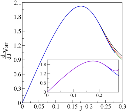
Figure 1: The first derivative of the variance of the on-site atom number occupation for the unit filling factor ($n=1$). Main plot: numerical results for system sizes $M=100$ (black), $200$ (red), $400$ (green), and $800$ (blue). Inset: the violet curve depicts the perturbative result obtained from (10) while the blue one shows $M=800$ data from the main plot. The two curves are practically indistinguishable for $J$ smaller than about $0.2$.

Second, insights into BKT physics of the 1D BH model can be also obtained from the single-particle energy gap, which is proportional to $\xi^{-1}(J)$. In addition to that, one may also study two-point correlation functions

$$\langle J|a^{\dagger}_{i+r}\hat{a}_{i}+\hat{a}^{\dagger}_{i}\hat{a}_{i+r}|J\rangle,$$ (8)

which for $r\gg 1$ are expected to exhibit the algebraic $r^{-1/4}$ decay at the BKT critical point (we overlook an essentially unobservable logarithmic correction to such a decay law, see e.g. Ref. Chaikin and Lubensky (1995)). Numerical studies of the former (latter) quantity can be found in Ref. Carrasquilla et al. (2013) (Refs. Kühner and Monien (1998); Kühner et al. (2000); Kub ; see also Ref. Rachel et al. (2012)). As far as experiments are concerned, it is unclear to us whether one can measure these quantities accurately-enough for getting conclusive insights into BKT physics. We mention in passing that more “exotic” physical quantities, providing insights complementary to the ones delivered by $d{\rm Var}/dJ$, will be commented upon in Secs. IV and V.

Third, experimental studies of BKT physics in cold atom setups were initiated by seminal work Hadzibabic et al. (2006). To the best of our knowledge, however, they were restricted to two-dimensional cold gases, where the classical BKT transition takes place (see e.g. Refs. Hadzibabic et al. (2006); Hung et al. (2011); Chomaz et al. (2015); Christodoulou et al. (2021) reporting experiments with either harmonically trapped or homogeneous Bose gases; see Ref. Hadzibabic and Dalibard (2011) for a review). Note that the quantum character of the BKT transition, 1D geometry, and the periodic lattice potential in our system strikingly contrast with the properties of the systems explored in these experimental works.

III Numerical simulations

Model (1), just as its two- and three-dimensional incarnations, is not exactly solvable. As a result, its theoretical studies are oftentimes carried out via numerical simulations. Our numerical simulations are presented in Figs. 1–3, showing the first, second, and third derivative of the variance in the Mott insulator phase (see Appendix B for technical details).

The most striking features seen on these figures are the extrema, whose location

$$\begin{array}[]{c|c|c}&\text{minimum}&\text{maximum}\\ \hline\cr d{\rm Var}/dJ&&0.176\\ \hline\cr d^{2}{\rm Var}/dJ^{2}&0.247&\\ \hline\cr d^{3}{\rm Var}/dJ^{3}&0.198&0.266\end{array}$$ (9)

is listed here for the largest system that we have numerically studied ($M=800$).

The broad maximum of $d{\rm Var}/dJ$, depicted in Fig. 1, is the quantum equivalent of the so-called non-universal specific heat peak that was predicted by the BKT theory (see e.g. Ref. Chaikin and Lubensky (1995), where such terminology is used in the classical context). Its off critical point location nicely illustrates the peculiar nature of BKT transitions. Indeed, in two- and three-dimensional BH models, where non-BKT transitions take place, $d{\rm Var}/dJ$ has maxima that are located at the critical points Łącki et al. (2016); Prośniak et al. (2019).

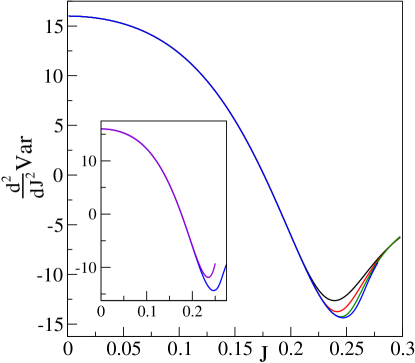
Figure 2: The same as in Fig. 1 except we deal here with the second derivative of the variance.

It is also evident from these figures that the non-universal contribution to the plotted quantities is by no means negligible at the critical point. This conclusion follows from the observation that all derivatives of (7) vanish at the critical point (${\cal E}_{\text{sing}}$ is essentially singular at $J_{c}$). Thus, derivatives of the variance at the critical point are entirely determined by the non-universal component of the ground state energy density. They are clearly far from being negligible there, which is seen after extrapolation of the data from Figs. 1–3 to $J=J_{c}\approx 0.3$ rem (b). Similar situation is found in classical BKT transitions, where the specific heat near critical points is known to be dominated by non-universal contributions Kosterlitz (2016).

We also note that finite-size effects are most evident near the maximum of the third derivative (Fig. 3). This is related to the fact that the correlation length of the infinite 1D BH model at $J=0.266$ is equal to about four hundred Rams et al. (2018), which is only a factor of two smaller than the largest system size that we have numerically studied.

Then, we compare numerical simulations to analytical results following from

$${\rm Var}(J) =8J^{2}-24J^{4}-\frac{2720}{9}J^{6}+\frac{70952}{81}J^{8}-\frac{176684}{81}J^{10}$$ (10)

$$+\frac{431428448}{6561}J^{12}+\frac{104271727762891}{330674400}J^{14}$$

$$+\frac{32507578587517774813}{3888730944000}J^{16}+O\!\left(J^{18}\right),$$

which was obtained via the Rayleigh-Schrödinger perturbative expansion in the tunneling coupling for an infinite system subjected to the unit filling factor constraint Damski and Zakrzewski (2015). We mention in passing that Ref. Damski and Zakrzewski (2015) comprehensively presents high-order perturbative studies of the Mott insulator phase of the 1D BH model (see also Refs. Freericks and Monien (1996); Elstner and Monien (1999); Mon ; Teichmann et al. (2009); Freericks et al. (2009); Ejima et al. (2012) for related albeit lower-order investigations).

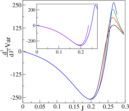
Figure 3: The same as in Fig. 1 except we deal here with the third derivative of the variance.

To begin, we take a look at positions of extrema following from (10). They are given by

$$\begin{array}[]{c|c|c}&\text{minimum}&\text{maximum}\\ \hline\cr d{\rm Var}/dJ&&0.176\\ \hline\cr d^{2}{\rm Var}/dJ^{2}&0.235&\\ \hline\cr d^{3}{\rm Var}/dJ^{3}&0.194&\end{array}\,,$$ (11)

which quite accurately reproduces all but one result reported in (9). The position of the maximum of the third derivative is missing here because such a maximum is absent in the third derivative of (10).

Next, we note that a very good agreement between numerics and perturbative results is seen for $J$ less than about $0.2$. This is sufficient for excellent (good) analytical characterization of the maximum (minimum) in Fig. 1 (Fig. 3). However, despite the high order of expansion (10), the shape of the minimum in Fig. 2 is only reasonably reproduced by the perturbative formula while the maximum in Fig. 3 is not captured by it, which we have already mentioned. This is presumably so because these two features are located at so large $J$ that a higher-order expansion is needed. For example, already near $J=0.2$, we can infer from the numerical data that the low order of the expansion, rather than finite-size effects, is responsible for discrepancies between numerics and analytics (the larger the system size is, the bigger they are).

The question now is how we can actually argue that the above-discussed numerics provides evidence of the quantum BKT transition taking place in our system. This brings us to the next section.

IV BKT fit

The idea here is to fit

$$\frac{d}{dJ}{\rm Var}(J)=-2J\frac{d^{2}}{dJ^{2}}\!\left[A\exp\!\left(-\frac{2B}{\sqrt{J_{c}-J}}\right)\right]+CJ+DJ^{2}$$ (12)

to numerics from Fig. 1, use so determined expression to compute higher derivatives of the variance, and finally to compare such obtained results for $d^{2}{\rm Var}/dJ^{2}$ and $d^{3}{\rm Var}/dJ^{3}$ to numerics presented in Figs. 2 and 3, respectively. Two remarks are in order now.

First, we set $J_{c}=0.3$ in (12), taking such a value from Ref. Krutitsky (2016). The fitting procedure yields the $A$, $B$, $C$, and $D$ coefficients. It will be applied to all data points that we have, which represent $d{\rm Var}/dJ$ in the Mott insulator phase. Such a choice of the range of $J$’s is motivated by the fact that the features that we try to capture, such as the maximum from Fig. 1, are not necessarily located near the critical point. Moreover, we reduce a bit arbitrariness of the fitting procedure by avoiding fine-tuning of the domain of (12).

Second, the exponential term in (12) comes from the universal BKT formula, see (6) and (7). The polynomial terms in (12) represent the non-universal contribution to $d{\rm Var}/dJ$ in the simplest possible way. This can be argued as follows. The constant, $J$-independent term is skipped as we expect from perturbative expansions that $d{\rm Var}/dJ$ vanishes at $J=0$. Both linear and quadratic terms in $J$ are needed for capturing the overall parabolic shape of the data from Fig. 1. Omission of the cubic, quartic, etc. terms in $J$ reduces the number of free parameters to minimum. Similar fitting schemes were explored in the classical context in Refs. Yu et al. (1989); Steele et al. (1993).

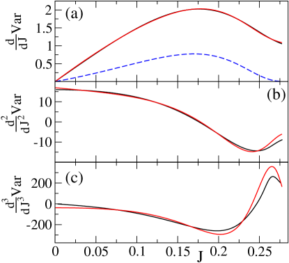
Figure 4: Comparison between numerics and the BKT fit discussed in Sec. IV. Black lines show numerics for the largest system that we consider ($M=800$). Red lines follow from (12) evaluated with the coefficients from (13). The dashed blue line in panel (a) depicts the universal part of the fitted function, i.e., the exponential contribution from (12). All results are for the unit filling factor ($n=1$).

The fitting has been done with the NonlinearModelFit function from Ref. Mat . It yielded

$$\begin{array}[]{c|c|c|c}A&B&C&D\\ \hline\cr-12.5(2)&1.465(3)&12.8(1)&-32.1(4)\end{array}\,,$$ (13)

where one standard error is listed in the brackets. All data from Fig. 1, for the $M=800$ system, has been used for the fit.

Out of these four fitting results, only the $B$ parameter can be compared to the former studies. Namely, it was extracted from numerical data for the single-particle energy gap, correlation length, ground state fidelity, and fidelity susceptibility of the 1D BH model Carrasquilla et al. (2013); Rams et al. (2018); Cincio et al. (2019). Those studies estimated it at $1.59(3)$, $1.61(4)$, $1.72(1)$, and $1.84(5)$, respectively. Our result adds one more value to the table, which does not seem to be solving the puzzle of what the value of $B$ really is. Given the fact that there is $25\%$ relative difference between the largest and the smallest reported value of $B$, further studies seem to be needed for tight estimation of this parameter.

The quality of the fit reported in (13) is depicted in Fig. 4a, where its good agreement with numerics is easily seen. We also separately plot there the universal contribution to the fitted expression. It is peaked near the maximum of $d{\rm Var}/dJ$, where it is of the same order of magnitude as the non-universal part of (12). Moreover, as Fig. 4a reveals, nowhere in the Mott insulator phase the universal contribution dominates over the non-universal one. This observation illustrates the curious nature of the studied transition, so much different from what one finds in standard, non-BKT, transitions.

Next, we combine (12) and (13) to compute higher derivatives of the variance and compare them to numerics in Figs. 4b and 4c. The agreement is good but not as good as in Fig. 4a. This is somewhat expected given the fact that we account for the non-universal part of the result with just a linear function ($C+2DJ$) in Fig. 4b and a constant term ($2D$) in Fig. 4c.

Having said all that, we can address the question posted by the end of Sec. III. Namely, we see agreement between curves plotted in Fig. 4 as solid evidence that there is a quantum BKT transition in our system. This remark should be especially convincing if one looks at Fig. 4c, where whole $J$-dependence comes solely from the universal BKT formula properly reproducing the shape of numerical data.

V Summary

We have discussed how BKT physics of the superfluid–Mott insulator quantum phase transition of the 1D BH model can be extracted from either the variance of the on-site atom number occupation or the nearest-neighbor correlation function. It may seem surprising at first glance that a clear signature of the BKT transition can be obtained from them. We say so because these two physical quantities seem to be featureless in the Mott insulator phase, where we do calculations (see e.g. Ref. Damski and Zakrzewski (2015)). Interestingly enough, this remark may explain the fact that we are unaware of any works discussing them from the BKT perspective.

A clear link to BKT physics appears when one considers the first derivative of the variance with respect to the parameter driving the transition. It turns out that such a quantity is the exact quantum analog of the specific heat (Sec. II). Thus, by studying it, we get direct insights into the quantum BKT transition from the same perspective from which classical BKT transitions are oftentimes discussed. The same can be said about the first derivative of the nearest-neighbor correlation function because it is proportional to the first derivative of the variance (Sec. II).

As far as experiments are concerned, both the variance and the nearest-neighbor correlation function can be measured (Sec. I). We expect that it should be also possible to extract their derivatives out of experimental data. In this context, we would like to mention Ref. Gerbier et al. (2005), where the derivative of experimentally-measured visibility of the time-of-flight interference pattern was used for estimation of critical points of the three-dimensional BH model. This work demonstrates feasibility of studies of derivatives of quantities measured in cold atom experiments.

It should be mentioned, however, that accurate computation of derivatives of experimental data would presumably require smoothing of such data first (e.g. by fitting some function to it). Once this would be done, calculation of derivatives should be easy. We have been able to avoid such a procedure in this work thanks to the high quality of numerical data that was differentiated (Appendix B). However, in our former studies, where Quantum Monte Carlo simulations were employed Łącki et al. (2016); Prośniak et al. (2019), we used the Padé approximant fitting approach.

After this qualitative overview, we would like to make the following comments.

First, we have studied systems with the average number of atoms per lattice site equal to either one (Secs. III and IV) or two (Appendix A). The latter case has been moved to the appendix because numerical results are similarly analyzed for both filling factors.

Second, we have discussed a scheme for extraction of BKT physics out of the above-mentioned observables (Sec. IV). By using it, we get to know how much the universal part contributes to the quantities that we study. For example, how much it contributes to the quantum analog of the so-called non-universal peak of the specific heat, which is depicted in Fig. 4a. We have shown that the universal component contributes to the peak about as much as the non-universal one. As a result of that, it seems to us that the peak in our system actually appears to be neither universal nor non-universal.

Third, it should be said that such a peak, to the best of our knowledge, was never experimentally observed in cold atom systems undergoing a quantum BKT transition.

Fourth, we are aware of just one earlier theoretical work on the 1D BH model, where some quantum analog of the specific heat peak was discussed from the BKT perspective Cincio et al. (2019). Its experimental exploration, however, asks for the measurement of either ground state fidelity or fidelity susceptibility. As far as we understand it, it is unclear how to measure the former, whereas the latter can be extracted from the measurements of the spectral function Gu and Yu (2014). It seems to us that the observables that we discuss are far more experimentally approachable.

Finally, we note that there are different versions of the 1D BH model presumably undergoing a quantum BKT transition Lewenstein et al. (2007); Dutta et al. (2015); Krutitsky (2016). We expect our ideas for studies of BKT physics to be also applicable to such models. We hope that this work will stimulate experimental exploration of cold-atom-based quantum BKT transitions.

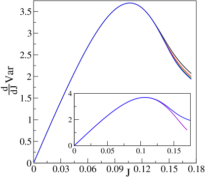
Figure 5: The first derivative of the variance of the on-site atom number occupation for the double filling factor ($n=2$). Main plot: numerical results for system sizes $M=100$ (black), $200$ (red), $400$ (green), and $800$ (blue). Inset: the violet curve depicts the perturbative result obtained from (14) while the blue one shows the $M=800$ data from the main plot. The two curves are nearly identical for $J$ smaller than about $0.1$.

Appendix A Double filling factor

The results for the filling factor $n=2$ are presented in Figs. 5–8. A quick comparison of Figs. 1–4 to Figs. 5–8 shows that qualitative features of derivatives of the variance are the same for filling factors $n=1,2$. As a result of that, we will just briefly summarize below quantitative features of the double filling factor results.

To begin, the relevant Rayleigh-Schrödinger perturbative expansion in the tunneling coupling now reads Damski and Zakrzewski (2015)

$${\rm Var}(J) =24J^{2}-192J^{4}-\frac{396832}{63}J^{6}$$ (14)

$$+\frac{6770645594}{496125}J^{8}-\frac{32931564509156}{9359398125}J^{10}$$

$$+\frac{7350064303936751836656911}{173664334164234375}J^{12}+O\!\left(J^{14}\right).$$

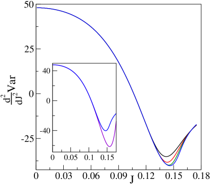
Figure 6: The same as in Fig. 5 except we deal here with the second derivative of the variance.

Extrema of numerical results, for the $M=800$ system, are characterized by

$$\begin{array}[]{c|c|c}&\text{minimum}&\text{maximum}\\ \hline\cr d{\rm Var}/dJ&&0.107\\ \hline\cr d^{2}{\rm Var}/dJ^{2}&0.146&\\ \hline\cr d^{3}{\rm Var}/dJ^{3}&0.118&0.157\end{array}$$ (15)

while the ones following from expansion (14) are

$$\begin{array}[]{c|c|c}&\text{minimum}&\text{maximum}\\ \hline\cr d{\rm Var}/dJ&&0.106\\ \hline\cr d^{2}{\rm Var}/dJ^{2}&0.157&\\ \hline\cr d^{3}{\rm Var}/dJ^{3}&0.128&\end{array}\,.$$ (16)

The position of the maximum of the third derivative is not listed in (16) because such a maximum is absent in the third derivative of (14).

Fitting of (12), to numerical data for the $M=800$ system in the range $0\leq J\leq 0.175$, has been done with $J_{c}=0.18$. Such a value of $J_{c}$ has been taken from the survey presented in Ref. Krutitsky (2016). We have obtained

$$\begin{array}[]{c|c|c|c}A&B&C&D\\ \hline\cr-13.2(2)&1.134(2)&38.7(3)&-157(2)\end{array}\,.$$ (17)

This time, however, the result for the parameter $B$ cannot be compared to the previous studies because we are unaware of any reference reporting it.

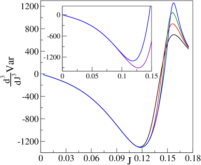
Figure 7: The same as in Fig. 5 except we deal here with the third derivative of the variance.

Appendix B Numerics

The ground state calculations have been performed using implementation of the Density Matrix Renormalization Group (DMRG) algorithm Schollwöck (2011) provided by the iTensor package Fishman et al. (2020). The numerical method minimizes the mean energy of variational many-body ground states expressed in the Matrix Product State (MPS) form. That representation is given by

$$|\psi_{\textrm{MPS}}\rangle=\sum_{i_{1},i_{2},\ldots,i_{M}}A^{[1]}_{i_{1}}A^{[2]}_{i_{2}}\cdots A^{[M]}_{i_{M}}|i_{1},i_{2},\ldots,i_{M}\rangle,$$ (18)

where $A^{[m]}_{i_{m}}$ are $1\times\chi$, $\chi\times\chi$, and $\chi\times 1$ matrices for $m=1$, $1<m<M$, and $m=M$, respectively. The index $i_{m}=0,1,\dots,7$ represents the on-site population of the $m$-th lattice site (we have checked that such a choice leads to well-converged results). The set of all states, for the given Schmidt dimension $\chi$, forms a variational manifold.

The MPS representation is exact for large-enough $\chi$. We have used $\chi=400$ for $M\leq 400$ and $\chi$ up to $1600$ for $M=800$. This concerns simulations at both the unit and double filling factors. Too small $\chi$ results in bad convergence of ground states, which translates into noise complicating calculations of derivatives. The sufficiently-large $\chi$ grows with $M$, making investigations of larger systems prohibitively expensive in terms of time and computer resources.

We have monitored the quality of our simulations by the study of discarded weights $w_{m}=\sum_{j>\chi}(\lambda_{j}^{[m]})^{2}$, where $\lambda_{j}^{[m]}$ are Schmidt coefficients Schollwöck (2011); Fishman et al. (2020). All simulated states have been converged down to $w_{m}\leq 10^{-10}$ for all $1\leq m\leq M$. The iTensor “cutoff” parameter, used for DMRG internal linear algebra truncation, has been set to $10^{-13}$ Fishman et al. (2020).

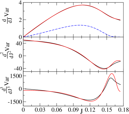
Figure 8: Comparison between numerics and the BKT fit for the double filling factor ($n=2$). Black lines show numerics for the $M=800$ system. Red lines follow from (12) evaluated with the coefficients from (17). The dashed blue line in the top panel depicts the universal part of the fitted function.

The variance has been computed from ground states, generated by the above-mentioned procedure for $J=\{J_{i}\}$, where $J_{i+1}-J_{i}=\delta\ll 1$. In order to minimize influence of open boundary conditions on our results, we have evaluated it at the central lattice site: ${\rm Var}=\langle\hat{n}^{2}_{M/2}\rangle-n^{2}$, where $n=1,2$. Its numerical derivatives have been obtained from the symmetric prescription

$$\frac{d}{dJ}{\rm Var}(J_{i+1/2})\approx\!\left[{\rm Var}(J_{i+1})-{\rm Var}(J_{i})\right]/\delta,$$ (19)

$$\frac{d^{2}}{dJ^{2}}{\rm Var}(J_{i})\approx\!\left[\frac{d}{dJ}{\rm Var}(J_{i+1/2})-\frac{d}{dJ}{\rm Var}(J_{i-1/2})\right]/\delta,$$ (20)

etc., where $J_{i+1/2}=J_{i}+\delta/2$.

From these formulae, one easily sees that the key limitation of such a procedure follows from the fact that the denominator of the $n$-th order derivative is given by $\delta^{n}$. This implies that reliable results are obtained only when accuracy of determination of ${\rm Var}(J_{i})$ is much better than $\delta^{n}$. To compute the first and second derivative of the variance, we have used $\delta=0.001$ getting smooth results. However, our results for the third derivative, obtained with such $\delta$, exhibit small fluctuations near the critical point due to worse accuracy of determination of the variance there. The problem with smoothness of the third derivative has been resolved by employment of $\delta=0.002$, which does not harm the overall accuracy of our studies as such $\delta$ is still sufficiently small.

Alternatively, one could have solved such an issue by differentiation of a smooth curve that has been fitted to ${\rm Var}(J_{i})$ data. We have not explored this option here because the above-mentioned procedure straightforwardly delivers good-quality results.

Finally, at the risk of stating the obvious, we mention that whole discussion from this appendix applies to our studies of both the unit and double filling factor systems.

References

- Lewenstein et al. (2007) M. Lewenstein, A. Sanpera, V. Ahufinger, B. Damski, A. Sen(De), and U. Sen, Adv. Phys. 56, 243 (2007).
- Bloch et al. (2008) I. Bloch, J. Dalibard, and W. Zwerger, Rev. Mod. Phys. 80, 885 (2008).
- Bloch et al. (2012) I. Bloch, J. Dalibard, and S. Nascimbène, Nat. Phys. 8, 267 (2012).
- Dutta et al. (2015) O. Dutta, M. Gajda, P. Hauke, M. Lewenstein, D.-S. Lühmann, B. A. Malomed, T. Sowiński, and J. Zakrzewski, Rep. Prog. Phys. 78, 066001 (2015).
- Krutitsky (2016) K. V. Krutitsky, Phys. Rep. 607, 1 (2016).
- Gross and Bloch (2017) C. Gross and I. Bloch, Science 357, 995 (2017).
- Coleman and Schofield (2005) P. Coleman and A. J. Schofield, Nature 433, 226 (2005).
- Sachdev and Keimer (2011) S. Sachdev and B. Keimer, Phys. Today 64, 29 (2011).
- Sachdev (2011) S. Sachdev, Quantum Phase Transitions (Cambridge University Press, Cambridge, 2011).
- Continentino (2017) M. Continentino, Quantum Scaling in Many-Body Systems: An Approach to Quantum Phase Transitions (Cambridge University Press, Cambridge, 2017), 2nd ed.
- (11) H. Ott, Rep. Prog. Phys. 79, 054401 (2016).
- Schäfer et al. (2020) F. Schäfer, T. Fukuhara, S. Sugawa, Y. Takasu, and Y. Takahashi, Nat. Rev. Phys. 2, 411 (2020).
- Nakamura et al. (2019) Y. Nakamura, Y. Takasu, J. Kobayashi, H. Asaka, Y. Fukushima, K. Inaba, M. Yamashita, and Y. Takahashi, Phys. Rev. A 99, 033609 (2019).
- Łącki et al. (2016) M. Łącki, B. Damski, and J. Zakrzewski, Sci. Rep. 6, 38340 (2016).
- Prośniak et al. (2019) O. A. Prośniak, M. Łącki, and B. Damski, Sci. Rep. 9, 8687 (2019).
- Jaksch et al. (1998) D. Jaksch, C. Bruder, J. I. Cirac, C. W. Gardiner, and P. Zoller, Phys. Rev. Lett. 81, 3108 (1998).
- (17) N. Navon R. P. Smith, Z. Hadzibabic, arXiv:2106.09716 (2021).
- Fisher et al. (1989) M. P. A. Fisher, P. B. Weichman, G. Grinstein, and D. S. Fisher, Phys. Rev. B 40, 546 (1989).
- rem (a) Phase transitions of both the -dimensional classical XY model and the -dimensional quantum BH model subjected to the integer filling factor constraint are known to belong to the same universality class (see e.g. seminal Ref. Fisher et al. (1989)).
- Berezinskii (1971) V. L. Berezinskii, Sov. Phys. JETP 32, 493 (1971).
- Berezinskii (1972) V. L. Berezinskii, Sov. Phys. JETP 34, 610 (1972).
- Kosterlitz and Thouless (1973) J. M. Kosterlitz and D. J. Thouless, J. Phys. C: Solid State Physics 6, 1181 (1973).
- Kosterlitz (2016) J. M. Kosterlitz, Rep. Prog. Phys. 79, 026001 (2016).
- van Oosten et al. (2001) D. van Oosten, P. van der Straten, and H. T. C. Stoof, Phys. Rev. A 63, 053601 (2001).
- Yu et al. (1989) Y. Y. Yu, D. Finotello, and F. M. Gasparini, Phys. Rev. B 39, 6519 (1989).
- Steele et al. (1993) L. M. Steele, C. J. Yeager, and D. Finotello, Phys. Rev. Lett. 71, 3673 (1993).
- Baxter (1982) R. J. Baxter, Exactly Solved Models in Statistical Mechanics (Academic Press, London, 1982).
- Chaikin and Lubensky (1995) P. M. Chaikin and T. C. Lubensky, Principles of Condensed Matter Physics (Cambridge University Press, 1995).
- Carrasquilla et al. (2013) J. Carrasquilla, S. R. Manmana, and M. Rigol, Phys. Rev. A 87, 043606 (2013).
- Kühner and Monien (1998) T. D. Kühner and H. Monien, Phys. Rev. B 58, R14741 (1998).
- Kühner et al. (2000) T. D. Kühner, S. R. White, and H. Monien, Phys. Rev. B 61, 12474 (2000).
- (32) J. Zakrzewski and D. Delande, Accurate determination of the superfluid-insulator transition in the one-dimensional Bose-Hubbard model, in Proceedings of Let’s Face Chaos Through Nonlinear Dynamics, 7th International Summer School and Conference, edited by M. Robnik and V. G. Romanovski, Vol. 1076 (AIP, Melville, NY, 2008), pp. 292–300; arXiv:cond-mat/0701739 (2007).
- Rachel et al. (2012) S. Rachel, N. Laflorencie, H. F. Song, and K. Le Hur, Phys. Rev. Lett. 108, 116401 (2012).
- Hadzibabic et al. (2006) Z. Hadzibabic, P. Krüger, M. Cheneau, B. Battelier, and J. Dalibard, Nature 441, 1118 (2006).
- Hung et al. (2011) C.-L. Hung, X. Zhang, N. Gemelke, and C. Chin, Nature 470, 236 (2011).
- Chomaz et al. (2015) L. Chomaz, L. Corman, T. Bienaimé, R. Desbuquois, C. Weitenberg, S. Nascimbène, J. Beugnon, and J. Dalibard, Nat. Commun. 6, 6162 (2015).
- Christodoulou et al. (2021) P. Christodoulou, M. Gałka, N. Dogra, R. Lopes, J. Schmitt, and Z. Hadzibabic, Nature 594, 191 (2021).
- Hadzibabic and Dalibard (2011) Z. Hadzibabic and J. Dalibard, Riv. Nuovo Cim. 34, 389 (2011).
- rem (b) Note that the non-zero value of derivatives of the variance at the critical point, suggested by extrapolation of the results from Figs. 1–3 to , cannot be attributed to finite-size effects, which are too small. The same can be said about the double filling factor case, which is depicted in Figs. 5–7.
- Rams et al. (2018) M. M. Rams, P. Czarnik, and L. Cincio, Phys. Rev. X 8, 041033 (2018).
- Damski and Zakrzewski (2015) B. Damski and J. Zakrzewski, New J. Phys. 17, 125010 (2015).
- Freericks and Monien (1996) J. K. Freericks and H. Monien, Phys. Rev. B 53, 2691 (1996).
- Elstner and Monien (1999) N. Elstner and H. Monien, Phys. Rev. B 59, 12184 (1999).
- (44) N. Elstner and H. Monien, arXiv:cond-mat/9905367 (1999).
- Teichmann et al. (2009) N. Teichmann, D. Hinrichs, M. Holthaus, and A. Eckardt, Phys. Rev. B 79, 224515 (2009).
- Freericks et al. (2009) J. K. Freericks, H. R. Krishnamurthy, Y. Kato, N. Kawashima, and N. Trivedi, Phys. Rev. A 79, 053631 (2009).
- Ejima et al. (2012) S. Ejima, H. Fehske, F. Gebhard, K. zu Münster, M. Knap, E. Arrigoni, and W. von der Linden, Phys. Rev. A 85, 053644 (2012).
- (48) Wolfram Research, Inc., Mathematica, Version 12.0, Champaign, IL (2019).
- Cincio et al. (2019) L. Cincio, M. M. Rams, J. Dziarmaga, and W. H. Zurek, Phys. Rev. B 100, 081108(R) (2019).
- Gerbier et al. (2005) F. Gerbier, A. Widera, S. Fölling, O. Mandel, T. Gericke, and I. Bloch, Phys. Rev. Lett. 95, 050404 (2005).
- Gu and Yu (2014) S.-J. Gu and W. C. Yu, EPL 108, 20002 (2014).
- Schollwöck (2011) U. Schollwöck, Ann. Phys. 326, 96 (2011).
- Fishman et al. (2020) M. Fishman, S. R. White, and E. M. Stoudenmire, arXiv:2007.14822 (2020).