Bilinear Control of Convection-Cooling: From Open-Loop to Closed-Loop

Abstract

This paper is concerned with a bilinear control problem for enhancing convection-cooling via an incompressible velocity field. Both optimal open-loop control and closed-loop feedback control designs are addressed. First and second order optimality conditions for characterizing the optimal solution are discussed. In particular, the method of instantaneous control is applied to establish the feedback laws. Moreover, the construction of feedback laws is also investigated by directly utilizing the optimality system with appropriate numerical discretization schemes. Computationally, it is much easier to implement the closed-loop feedback control than the optimal open-loop control, as the latter requires to solve the state equations forward in time, coupled with the adjoint equations backward in time together with a nonlinear optimality condition. Rigorous analysis and numerical experiments are presented to demonstrate our ideas and validate the efficacy of the control designs.

1 Introduction

The question of the influence of advection on diffusion is a topic of fundamental interest in engineering and natural sciences with broad applications ranging from heat transfer, chemical mixing on small and large scales, to preventing the spreading of pollutants in geophysical flows. Convection-cooling is the mechanism where heat is transferred from a hot object into the ambient air or liquid. In general, there are two types of convectional cooling: natural convection cooling and the forced air convection cooling (cf. [4, 2, 39]). The latter is used in designs where the enclosures or environment do not offer an effective natural cooling performance. In this work, we are aiming at understanding what flows are efficient in enhancing cooling or the homogenization process and whether it is possible to construct such flows by utilizing the information of the temperature only. Specifically, we are interested in the control designs for convection-cooling via incompressible fluid flows. To this end, we consider the diffusion-convection model for a cooling application in an open bounded and connected domain $\Omega\subset\mathbb{R}^{d},d=2,3$, with a Lipschitz boundary $\Gamma$. The system of equations reads

$$\frac{\partial T}{\partial t} =\kappa\Delta T-\mathbf{v}\cdot\nabla T\quad\text{in}\quad\Omega,$$ (1.1)

$$\nabla\cdot\mathbf{v} =0\quad\text{in}\quad\Omega,$$ (1.2)

where $T$ is the temperature, $\kappa>0$ is the thermal diffusivity, and $\mathbf{v}$ is a divergence free vector field. Neumann boundary condition for temperature and no-slip boundary condition for velocity are considered, i.e.,

$$\frac{\partial T}{\partial n}\Big{|}_{\Gamma}=0\quad\text{and}\quad\mathbf{v}|_{\Gamma}=0.$$ (1.3)

The initial condition is given by

$$T(x,0)=T_{0}(x).$$ (1.4)

The diffusion-convection model (1.1)–(1.4) is one of the most studied PDEs in both mathematical and physical literature. Of special note is that the flow velocity will be taken as the control input in this work. This naturally leads to a bilinear control problem. In particular, we like to understand what is the optimal flow velocity that accelerates the convergence of the temperature to its average, and construct such velocity in a feedback form. Constantin et al. in [16] provided a sharp characterization of incompressible flows that produce a significantly stronger dissipative effect than dissipation alone. However, constructing an optimal velocity field in a feedback form is non-trivial. One of the well-known approaches is to solve the related Hamilton-Jacobi-Bellam (HJB) differential equation, yet it suffers the curse of dimensionality. In this work, we are aiming at investigating a feasible nonlinear feedback control law for convection-cooling based on the instantaneous control design and establish the corresponding stabilization results. The fundamental idea of instantaneous control is built upon an optimal control problem, which essentially gives rise to a sub-optimal feedback law. Moreover, we also investigate the construction of feedback laws directly utilizing the discretized optimality conditions. As a first step to implement the feedback control design, we start with an optimal control problem seeking for a velocity field that minimizes the variance of the temperature distribution. The problem can be formulated as follows: find an incompressible velocity $\mathbf{v}$ that minimizes

$$J(\mathbf{v}) =\frac{\alpha}{2}\|T(x,t_{f})-\langle T(x,t_{f})\rangle\|^{2}_{L^{2}}+\frac{\beta}{2}\int^{t_{f}}_{0}\|T-\langle T\rangle\|^{2}_{L^{2}}\,dt+\frac{\gamma}{2}\|\mathbf{v}\|^{2}_{U_{\text{ad}}}$$ (P)

for a given $t_{f}>0$, subject to (1.1)–(1.4), where $\langle T\rangle=\frac{1}{|\Omega|}\int_{\Omega}T\,dx$ stands for the spatial average of temperature, $\alpha,\beta\geq 0$ and $\gamma>0$ are the state and control weight parameters, respectively, and $U_{\text{ad}}$ stands for the set of admissible control. The parameters $\alpha$ and $\beta$ do not vanish simultaneously.

For the convenience of our discussion, we first introduce the following spaces

$$H =\{\mathbf{v}\in L^{2}(\Omega)\colon\nabla\cdot\mathbf{v}=0,\ \mathbf{v}\cdot n|_{\Gamma}=0\},\qquad V=\{\mathbf{v}\in H^{1}_{0}(\Omega)\colon\nabla\cdot\mathbf{v}=0\}.$$

The most relevant work on optimal control of the scalar field via incompressible fluid flows can be found in (cf. [44, 1, 31, 32, 33, 34, 35, 36, 25, 37]), with applications to heat transfer, fluid mixing and optical flow control problems. Due to the advection term $\mathbf{v}\cdot\nabla T$, the control-to-state map $\mathbf{v}\mapsto T$ is bilinear, and hence problem (P) becomes non-convex and the optimal solution may not be unique in general. The choice of $U_{\text{ad}}$ plays a key role in proving the existence of an optimal solution and deriving the optimality conditions. Establishing the existence of an optimal velocity field will involve a compactness argument associated with the control-to-state map. To obtain a steady flow, Liu in [44] penalized the magnitude of the time derivative of $\mathbf{v}$ in the cost functional, however, this resulted in a nonlinear wave type of optimality conditions, which are difficult to implement numerically. Barbu and Marinoschi in [1] showed the existence of an optimal solution for $\mathbf{v}\in L^{2}(0,t_{f};H)$, yet the challenge was encountered in deriving the first order optimality conditions. For $\mathbf{v}\in L^{2}(0,t_{f};H)$, it is not smooth enough to allow the differentiability of the state equations. Consequently, the variational inequality or the Euler-Lagrange method can not be directly applied. Instead, an approximating control approach was employed in [1], which first considered the velocity in a much smoother space and then showed the convergence of the optimality conditions for the approximating control problem to the original one. Moreover, as shown in [1, Theorem 6], if further assume that $\mathbf{v}\in L^{\infty}(0,t_{f};L^{\infty}(\Omega)\cap H)$, then the uniqueness of the optimal controller can be obtained by showing the uniqueness of the optimality system under certain conditions. Similar ideas have been adopted in (cf. [35, 36]). A recent work by Glowinski et al. in [25] has conducted a numerical study on optimization algorithms for solving problem (P).

Motivated by the need of reducing the effects of rotation on the flow and the shear stress at the boundary in the cooling process, in this work we are interested in minimizing the magnitude of the strain tensor (cf. [21, 44]), which is equivalent to minimize $\|\nabla\mathbf{v}\|_{L^{2}}$. In this case, we set

$$U_{\text{ad}}=L^{2}(0,t_{f};V)$$ (1.5)

equipped with the norm $\|\mathbf{v}\|_{U_{\text{ad}}}=\|\mathbf{v}\|_{L^{2}(0,t_{f};H^{1}(\Omega))}.$ The regularity of $U_{\text{ad}}$ defined by (1.5) will allow us to carry out the G$\hat{a}$teaux differentiability of the state equations. Then the optimality conditions can be established by directly employing a variational inequality or the Euler-Lagrange method. However, to numerically implement the resulting optimality system for problem (P), one has to solve the state equations forward in time, coupled with the adjoint equations backward in time together with a nonlinear optimality condition. Straightforward use of this result can result in extremely high computational costs. Instantaneous control design is a powerful tool for dealing with the computational limitations of open-loop control, while providing a feedback law for flow control problems at a sustainable control cost (cf. [12, 30, 28, 8, 14, 53]). The idea behind it is that it successively determines approximations of the objective function while marching forward in time. The uncontrolled dynamical system is first discretized in time. Then, at selected time slices an instantaneous version of the cost functional is approximately minimized subject to a stationary system, whose structure depends on the chosen discretization method. The control obtained is used to steer the system to the next time slice, where the procedure is repeated (cf. [30]). This method is closely tied to receding horizon control (RHC) or model predictive control (MPC) with finite time horizon (cf. [22, 46, 47, 3]). Essentially, instantaneous control is a discrete-in-time and suboptimal feedback control approach and can be interpreted as the stable time discretization of a closed-loop control law (cf. [13, 40, 30, 28, 45, 27]). On the other hand, given the optimality system, it is natural to ask whether it is possible to obtain the equivalent feedback laws by first solving it restricted to each time slice and then marching forward in time. Following the convention, without any ambiguity, we will call the former “discretize-then-optimize (DTO)” approach and the latter “optimize-then-discretize (OTD)” approach in this work.

The remainder of this paper is organized as follows. In section 2, the first order optimality conditions are established for solving an optimal solution using a variational inequality (cf. [41]). Then the second order necessary conditions are derived to charactering the solution when the control weight $\gamma$ is sufficiently large. In section 3, the feedback control is constructed using both DTO and OTD approaches, which turn out to be the same feedback law under appropriate discretization schemes. The well-posedness and asymptotic behavior of the closed-loop system will be also addressed. Numerical implementation of our control designs are presented in section 4, where several numerical experiments are conducted to compare the effectiveness of the optimal control and the feedback control for convection-cooling.

In the sequel, the symbol $C$ denotes a generic positive constant, which is allowed to depend on the domain as well as on indicated parameters without ambiguous.

2 Existence and Optimality Conditions

In this section, we discuss the existence of an optimal solution to problem (P) and derive the first and second order optimality conditions for characterizing the optimal control by utilizing a variational inequality (cf. [41]).

Theorem 2.1.

For $T_{0}\in L^{\infty}(\Omega)$, there exists at least one optimal solution $\mathbf{v}\in U_{\text{ad}}$ to problem (P).

The proof of the existence for $\mathbf{v}\in U_{\text{ad}}$ follows the similar approaches as in [1, Theorem 1] for $\mathbf{v}\in L^{2}(0,t_{f};H)$. The details are omitted here. To establish the optimality conditions, however, it is critical to understand the regularity properties of the solution to the state equations for $\mathbf{v}\in U_{\text{ad}}$.

The following results will be often used in this work. The detailed proof of next lemma can be found in (cf. [51]).

Lemma 2.2.

Let $\mathbf{v}\in L^{2}(0;t_{f};H^{1}(\Omega),d=2,3$, $\phi\in L^{2}(0;t_{f};H^{1}(\Omega))$, and $\psi\in H^{1}(\Omega)$. Then we have

$$\left|\int_{\Omega}(\mathbf{v}\cdot\nabla\phi)\psi\,dx\right|\leq\|\mathbf{v}\|_{L^{4}}\|\nabla\phi\|_{L^{2}}\|\psi\|_{L^{4}}\leq C\|\nabla\mathbf{v}\|_{L^{2}}\|\nabla\phi\|_{L^{2}}\|\nabla\psi\|_{L^{2}},$$ (2.1)

and hence,

$$\mathbf{v}\cdot\nabla\phi\in L^{1}(0,t_{f};(H^{1}(\Omega))^{\prime}).$$ (2.2)

Moreover, if $\nabla\cdot\mathbf{v}=0$ and $\mathbf{v}|_{\Gamma}=0$, then

$$\int_{\Omega}(\mathbf{v}\cdot\nabla\phi)\psi\,dx=-\int_{\Omega}\phi\mathbf{v}\cdot\nabla\psi\,dx.$$ (2.3)

In addition, since the velocity field is incompressible with no-slip boundary condition, it is easy to check that given zero Neumann boundary condition, the average of the temperature satisfies

$$\langle T\rangle=\langle T_{0}\rangle,\quad\forall t\in[0,t_{f}].$$ (2.4)

In fact, taking the integral of (1.1) over $\Omega$ and applying Stokes formula (cf. [51]) together with (1.2)–(1.3) yields

$$\frac{d}{dt}\left(\int_{\Omega}T\,dx\right) =\kappa\int_{\Omega}\Delta T\,dx-\int_{\Omega}\mathbf{v}\cdot\nabla T\,dx=\kappa\int_{\Gamma}\frac{\partial T}{\partial n}\,dx-\int_{\Gamma}(\mathbf{v}\cdot n)T\,dx+\int_{\Omega}(\nabla\cdot\mathbf{v})T\,dx=0,$$

and therefore (2.4) follows.

Lemma 2.3.

Let $T_{0}\in L^{\infty}(\Omega)\cap H^{1}(\Omega)$. For $\mathbf{v}\in U_{\text{ad}}$, there exists a unique solution to the state equations (1.1)–(1.3), which satisfies

$$T\in(L^{\infty}(0,t_{f};L^{\infty}(\Omega)\cap H^{1}(\Omega))\cap L^{2}(0,t_{f};H^{2}(\Omega)).$$ (2.5)

Proof.

For $T_{0}\in L^{\infty}(\Omega)$ and $\mathbf{v}\in L^{2}(0,t_{f};H)$, the existence of a unique weak solution $T$ to (1.1)–(1.4) has been shown in [1, Theorem 1]. Moreover,

$$T\in C([0,t_{f}];L^{2}(\Omega))\cap L^{2}(0,t_{f};H^{1}(\Omega))\cap L^{\infty}(0,t_{f};L^{\infty}(\Omega)).$$ (2.6)

To see (2.6), taking the inner product of (1.1) with $T$ and integrating by parts using (1.3), we have

$$\frac{1}{2}\frac{d\|T\|^{2}_{L^{2}}}{dt}+\kappa\|\nabla T\|^{2}_{L^{2}}=-\int_{\Omega}(\mathbf{v}\cdot\nabla T)T\,dx=-\frac{1}{2}\int_{\Omega}\mathbf{v}\cdot\nabla(T^{2})\,dx=-\frac{1}{2}\left(\int_{\Gamma}(\mathbf{v}\cdot n)\,T^{2}\,dx-\int_{\Omega}(\nabla\cdot\mathbf{v})\,T^{2}\,dx\right)=0,$$ (2.7)

which gives

$$\|T\|^{2}_{L^{2}}+2\kappa\int^{t}_{0}\|\nabla T\|^{2}_{L^{2}}\,dt=\|T_{0}\|^{2}_{L^{2}},\quad t\in[0,t_{f}].$$ (2.8)

Furthermore, since $\frac{\partial T}{\partial t}\in L^{2}(0,t_{f};(H^{1}(\Omega))^{\prime})$, by Aubin-Lions Lemma we have $T\in C([0,t_{f}];L^{2}(\Omega))$.

Analogously, taking the inner product of (1.1) with $T^{N-1}$ with $N\geq 2$ and then letting $N\to\infty$ we get

$$\sup_{t\in[0,t_{f}]}\|T\|_{L^{\infty}}\leq\|T_{0}\|_{L^{\infty}}.$$ (2.9)

This estimate can be achieved by using the Stampacchia theory. The reader is referred to [1, 49] for details. To see (2.5), taking the inner product of (1.1) with $-\Delta T$ and using Green’s formula follow

$$\frac{1}{2}\frac{d\|\nabla T\|^{2}_{L^{2}}}{dt}+\kappa\|\Delta T\|^{2}_{L^{2}}=-\int_{\Omega}\nabla(\mathbf{v}\cdot\nabla T)\cdot\nabla T\,dx$$ (2.10)

$$=-\int_{\Omega}\partial_{j}v_{i}\partial_{i}T\partial_{j}T\,dx-\frac{1}{2}\int_{\Omega}v_{i}\partial_{i}(\partial_{j}T\partial_{j}T)\,dx$$ (2.11)

$$=-\int_{\Omega}\partial_{j}v_{i}\partial_{i}T\partial_{j}T\,dx-\frac{1}{2}\left(\int_{\Gamma}v_{i}n_{i}(\partial_{j}T\partial_{j}T)\,dx-\int_{\Omega}\partial_{i}v_{i}(\partial_{j}T\partial_{j}T)\,dx\right)$$

$$=-\int_{\Omega}\partial_{j}v_{i}\partial_{i}T\partial_{j}T\,dx\leq\|\nabla\mathbf{v}\|_{L^{2}}\|\nabla T\|^{2}_{L^{4}}\leq C\|\nabla\mathbf{v}\|_{L^{2}}\|\nabla T\|_{L^{2}}\|\Delta T\|_{L^{2}}$$

$$\leq C\|\nabla\mathbf{v}\|^{2}_{L^{2}}\|\nabla T\|^{2}_{L^{2}}+\frac{\kappa}{2}\|\Delta T\|^{2}_{L^{2}},$$ (2.12)

where from (2.10) to (2.11) we used Einstein’s summation convection, i.e., $\nabla(\mathbf{v}\cdot\nabla T)\cdot\nabla T=\partial_{j}(v_{i}\partial_{i}T)\partial_{j}T$. From (2.12) we get

$$\frac{d\|\nabla T\|^{2}_{L^{2}}}{dt}+\kappa\|\Delta T\|^{2}_{L^{2}}\leq C\|\nabla\mathbf{v}\|^{2}_{L^{2}}\|\nabla T\|^{2}_{L^{2}},$$ (2.13)

and hence, using Grönwall’s inequality gives

$$\sup_{t\in[0,t_{f}]}\|\nabla T\|_{L^{2}}\leq e^{C\int^{t_{f}}_{0}\|\nabla\mathbf{v}\|^{2}_{L^{2}}\,dt}\|\nabla T_{0}\|_{L^{2}}<\infty.$$ (2.14)

Moreover, from (2.13) we have

$$\kappa\int^{t_{f}}_{0}\|\Delta T\|^{2}_{L^{2}}\,dt\leq C\int^{t_{f}}_{0}\|\nabla\mathbf{v}\|^{2}_{L^{2}}\|\nabla T\|^{2}_{L^{2}}\,dt\leq C\|\mathbf{v}\|^{2}_{U_{\text{ad}}}\sup_{t\in[0,t_{f}]}\|\nabla T\|_{L^{2}}<\infty,$$

which completes the proof. ∎

2.1 Optimality Conditions

Let $A=-\mathbb{P}\Delta$ be the Stokes operator with $D(A)=V\cap H^{2}(\Omega),$ where $\mathbb{P}\colon L^{2}(\Omega)\to H$ is the Leray projector (cf. [15, p. 31]). Note that $A$ is a strictly positive and self-adjoint operator. Moreover, define $D\colon L^{2}(\Omega)\to L^{2}(\Omega)$ such that $DT=T-\langle T\rangle$. Then the cost functional is equivalent to

$$J(\mathbf{v}) =\frac{\alpha}{2}\|DT(t_{f})\|^{2}_{L^{2}}+\frac{\beta}{2}\int^{t_{f}}_{0}(D^{*}DT,T)\,dt+\frac{\gamma}{2}\int^{t_{f}}_{0}(A\mathbf{v},\mathbf{v})\,dt.$$ (2.15)

As shown in [37], it is easy to versify that $D=D^{*}$ and $D^{2}=D$, thus $\|D\|\leq 1$.

Now we derive the first order necessary optimality conditions for problem (P) by using a variational inequality (cf. [41]), that is, if $\mathbf{v}$ is an optimal solution of problem (P), then there holds

$$J^{\prime}(\mathbf{v})\cdot(\mathbf{w}-\mathbf{v})\geq 0,\quad\mathbf{w}\in U_{\text{ad}}.$$ (2.16)

To establish the G$\hat{a}$teaux differentiability of $J(\mathbf{v})$, we first check the G$\hat{a}$teaux differentiability of $T$ with respect to $\mathbf{v}$. Let $z$ be the G$\hat{a}$teaux derivative of $T$ with respect to $\mathbf{v}$ in the direction of $h\in U_{\text{ad}}$, i.e., $z=T^{\prime}(\mathbf{v})\cdot h$. Then $z$ satisfies

$$\begin{split}\frac{\partial z}{\partial t}&=\kappa\Delta z-\mathbf{v}\cdot\nabla z-h\cdot\nabla T,\quad\frac{\partial z}{\partial n}\Big{|}_{\Gamma}=0,\end{split}$$ (2.17)

with $z(x,0)=0$. To show existence of (2.17), we first establish an a prior estimate of $z$. Taking the inner product of (2.17) with $z$ and applying (2.3), we get

$$\frac{1}{2}\frac{d\|z\|^{2}_{L^{2}}}{dt}+\kappa\|\nabla z\|^{2}_{L^{2}} =\int_{\Omega}T(h\cdot\nabla z)\,dx\leq\|T\|_{L^{\infty}}\|h\|_{L^{2}}\|\nabla z\|_{L^{2}}$$

$$\quad\leq\frac{1}{2\kappa}\|T\|^{2}_{L^{\infty}}\|h\|^{2}_{L^{2}}+\frac{\kappa}{2}\|\nabla z\|^{2}_{L^{2}},$$

which follows

$$\frac{d\|z\|^{2}_{L^{2}}}{dt}+\kappa\|\nabla z\|^{2}_{L^{2}}\leq\frac{1}{\kappa}\|T\|^{2}_{L^{\infty}}\|h\|^{2}_{L^{2}}.$$

With the help of Lemma 2.2 and (2.8) we have

$$\|z\|^{2}_{L^{2}}+\kappa\int^{t}_{0}\|\nabla z\|^{2}_{L^{2}}\,ds\leq\frac{1}{\kappa}\int^{t}_{0}\|T\|^{2}_{L^{\infty}}\|h\|^{2}_{L^{2}}\,ds\leq\frac{C}{\kappa}\|T_{0}\|^{2}_{L^{\infty}}\|h\|^{2}_{U_{\text{ad}}},\quad t\in[0,t_{f}].$$ (2.18)

Based on Lemma 2.2, (2.8) and (2.18), it is clear that $\mathbf{v}\cdot\nabla z$ and $h\cdot\nabla T\in L^{1}(0,t_{f};H^{-1}(\Omega))$, thus $\frac{\partial z}{\partial t}\in L^{1}(0,t_{f};H^{-1}(\Omega))$. According to [51, Theorem 3.1], there exists a unique solution to (2.17) and $z\in L^{\infty}(0,t_{f};L^{2}(\Omega))\cap L^{2}(0,t_{f};H^{1}(\Omega))$. Therefore, $T(\mathbf{v})$ is G$\hat{a}$teaux differentiable for $\mathbf{v}\in U_{\text{ad}}$, so is $J(\mathbf{v})$.

The following theorem establishes the first order optimality conditions for the solving the optimal control.

Theorem 2.4.

If $\mathbf{v}$ is the optimal solution to problem (P) and $T$ is the corresponding solution to the state equations (1.1)–(1.4). Then there exists an adjoint state $q$ such that the optimal triplet $(\mathbf{v},T,q)$ satisfies

$$\frac{\partial T}{\partial t}=\kappa\Delta T-\mathbf{v}\cdot\nabla T,\quad\frac{\partial T}{\partial n}\Big{|}_{\Gamma}=0,\quad T(0)=T_{0},$$ (2.19)

$$-\frac{\partial q}{\partial t}=\kappa\Delta q+{\mathbf{v}}\cdot\nabla q+\beta D^{*}DT,\quad\frac{\partial q}{\partial n}\Big{|}_{\Gamma}=0,\quad q(t_{f})=\alpha D^{*}DT(t_{f}),$$ (2.20)

$$-\gamma\Delta{\mathbf{v}}+\nabla p=q\nabla T,\quad\nabla\cdot\mathbf{v}=0,\quad\mathbf{v}|_{\Gamma}=0,$$ (2.21)

where pressure $p\in L^{2}(\Omega)$ satisfies $\int_{\Omega}p\,dx=0$.

Proof.

The first order necessary optimality system for $\mathbf{v}\in L^{2}(0,t_{f};H)$ has been derived in [1, Theorem] using an approximate control approach. However, since $J$ is G$\hat{a}$teaux differentiable for $\mathbf{v}\in U_{\text{ad}}$ in our current work as shown in Theorem 2.4, we are able to directly apply the variational inequality (2.16) to establish this result.

First multiply (2.17) by $q$ and integrate over $\Omega\times(0,t_{f})$. Then applying integration by parts and Green’s formula together with (2.3), we have

$$(z(t_{f}),q(t_{f}))-\int^{t_{f}}_{0}(z,\frac{\partial q}{\partial t})\,dt =\int^{t_{f}}_{0}(z,\kappa\Delta q)\,dt+\int^{t_{f}}_{0}(z,{\mathbf{v}}\cdot\nabla q)\,dt.$$

On the other hand,

$$J^{\prime}(\mathbf{v})\cdot h= \alpha(D^{*}DT(t_{f}),z(t_{f}))+\beta\int^{t_{f}}_{0}(D^{*}DT,z)\,dt+\gamma\int^{t_{f}}_{0}(A\mathbf{v},h)\,dt.$$ (2.22)

Now let the adjoint state $q$ satisfy (2.20). The Gâteaux derivative of $J$ becomes

$$J^{\prime}(\mathbf{v})\cdot h= (q(t_{f}),z(t_{f}))-\int^{t_{f}}_{0}(\frac{\partial q}{\partial t}+\kappa\Delta q+\mathbf{v}\cdot\nabla q,z)\,dt+\gamma\int^{t_{f}}_{0}(A\mathbf{v},h)\,dt$$

$$= \int^{t_{f}}_{0}(q,\frac{\partial z}{\partial t}-\kappa\Delta z+\mathbf{v}\cdot\nabla z)\,dt+\gamma\int^{t_{f}}_{0}(A\mathbf{v},h)\,dt$$

$$= \int^{t_{f}}_{0}(q,-h\cdot\nabla T)\,dt+\gamma\int^{t_{f}}_{0}(A\mathbf{v},h)\,dt$$

$$= \int^{t_{f}}_{0}(-q\nabla T,h)\,dt+\gamma\int^{t_{f}}_{0}(A\mathbf{v},h)\,dt.$$ (2.23)

Therefore, if $\mathbf{v}^{\text{opt}}$ is the optimal solution, then $J^{\prime}(\mathbf{v}^{\text{opt}})\cdot h\geq 0$ for any $h\in U_{\text{ad}}$. This implies

$$\gamma A\mathbf{v}^{\text{opt}}-\mathbb{P}(q\nabla T)=0\quad\text{or}\quad-\gamma\Delta\mathbf{v}^{\text{opt}}+\nabla p-q\nabla T=0$$ (2.24)

for some $p\in L^{2}(\Omega)$ with $\int_{\Omega}p\,dx=0$.

Moreover, applying the similar approaches as in Lemma 2.3 and (2.9) and noting that $\|D\|\leq 1$, we have

$$\|q\|^{2}_{L^{2}}+2\kappa\int^{t}_{0}\|\nabla q\|^{2}_{L^{2}}\leq\beta\int^{t_{f}}_{0}\|T\|^{2}_{L^{2}}\,dt+\alpha\|T(t_{f})\|^{2}_{L^{2}}\leq C(T_{0},t_{f}),\quad t\in[0,t_{f}],$$ (2.25)

$$\text{and}\quad\sup_{t\in[0,t_{f}]}\|q\|_{L^{\infty}}\leq\beta\int^{t_{f}}_{0}\|T\|_{L^{\infty}}\,dt+\alpha\|T(t_{f})\|_{L^{\infty}}\leq C(T_{0},t_{f}),$$ (2.26)

for some constant $C(T_{0},t_{f})$ depending on $T_{0}$ and $t_{f}$. This completes the proof. ∎

Note that the uniqueness of the solution to the optimality system (2.19)–(2.21) can be obtained under certain conditions on $T_{0},t_{f}$ and $\gamma$. The proof follows the same as in [1, Theorem 6]. Moreover, we have the following regularity results for any optimal triplet $(\mathbf{v},T,q)$ satisfying (2.19)–(2.21). The proof is presented in Appendix Appendix.

Corollary 2.5.

If $T_{0}\in H^{2}(\Omega)$ and $(\mathbf{v},T,q)$ satisfies the first order necessary optimality system (2.19)–(2.21), then

$$\mathbf{v}\in L^{\infty}(0,t_{f};V\cap H^{2}(\Omega)),\quad T\in L^{\infty}(0,t_{f};H^{2}(\Omega))\cap L^{2}(0,t_{f};H^{3}(\Omega)).$$ (2.27)

With the help of these properties, we can further address the second order necessary optimality conditions for characterizing the optimal solutions.

Theorem 2.6.

Let $\mathbf{v}$ be an optimal solution to problem (P) and the triplet $(\mathbf{v},T,q)$ satisfy the first order necessary optimality system (2.19)–(2.21). If $\gamma>0$ is sufficiently large, then there exists some constant $c_{0}>0$ such that

$$J^{\prime\prime}(\mathbf{v})\cdot(h,h)\geq c_{0}\|h\|^{2}_{U_{\text{ad}}},$$ (2.28)

for $h\in U_{\text{ad}}$.

The proof of Theorem 2.6 is given in Appendix Appendix. However, the regularity of $U_{\text{ad}}$ is not sufficient for $J$ to have the twice G$\hat{a}$teaux differentiability in general.

3 Feedback Control Law Based on Instantaneous Control Design

With the understanding of the optimal control design in our disposal, we are in the position to construct a feedback control law based on the method of instantaneous control and compare the DTO approach with the OTD approach. The former, as mentioned earlier, is to first discretize the uncontrolled state equations in time and conduct the optimization procedure over discrete time steps, and then progress recursively in time (cf. [28, 30]). In contrast, the latter is to directly discretize the optimality system (2.19)–(2.21) on one step time sub-interval, and then carry the information for the next time sub-interval, where the state and the adjoint equations will be formulated forward and backward in time, respectively, but just for one step. Finally, we observe that under appropriate time discretization schemes, these two approaches lead to the same nonlinear continuous feedback controller. Its effectiveness will be compared with the optimal control numerically in section 4.

3.1 Discretize-then-Optimize Approach

Consider a uniform partition of $[0,t_{f}]$ and let $\tau=\frac{t_{f}}{n+1}$ for $n\in\mathbb{N}$ and $t_{i}=i\tau,i=0,1,\dots,n$. Using the semi-implict Euler’s method for discretizing the state equations (1.1) in time gives, for $i=0,1,\dots,n$,

$$\frac{T^{i+1}-T^{i}}{\tau}=\kappa\Delta T^{i+1}-\mathbf{v}^{i+1}\cdot\nabla T^{i},\quad\text{that is}\quad(I-\kappa\tau\Delta)T^{i+1}=T^{i}-\tau\mathbf{v}^{i+1}\cdot\nabla T^{i},$$ (3.1)

where $T^{0}=T_{0}$. Let $\alpha=0$, $\beta=1$, $U^{i}_{\text{ad}}=V$, and $\langle T^{i+1}\rangle=\frac{1}{\tau}\int^{t_{i+1}}_{t_{i}}\langle T\rangle\,ds$. Given $T^{i}$ at $t_{i}$, we solve for the control $\mathbf{v}^{i+1}$ at $t_{i+1}$ by minimizing the following instantaneous version of the cost functional $J$ in ($P$):

$$J^{i+1}(\mathbf{v}^{i+1}) =\frac{1}{2}\int_{\Omega}|T^{i+1}-\langle T^{i+1}\rangle|^{2}\,dx+\frac{\gamma}{2}\int_{\Omega}|A^{1/2}\mathbf{v}^{i+1}|^{2}\,dx$$

$$=\frac{1}{2}(D^{*}DT^{i+1},T^{i+1})+\frac{\gamma}{2}(A\mathbf{v}^{i+1},\mathbf{v}^{i+1})\hskip 72.26999pt P^{i+1}$$ ()

subject to (3.1). Again using a similar variational inequality as shown in proof of Theorem 2.4, we have

$$(J^{i+1})^{\prime}(\mathbf{v}^{i+1})\cdot h^{i+1} =(D^{*}DT^{i+1},z^{i+1})+\gamma(A\mathbf{v}^{i+1},h^{i+1})$$

for $h^{i+1}\in U^{i+1}_{\text{ad}}$, where $z^{i+1}=(T^{i+1})^{\prime}(\mathbf{v}^{i+1})\cdot h^{i+1}$ satisfies

$$(I-\kappa\tau\Delta)z^{i+1}=-\tau h^{i+1}\cdot\nabla T^{i},\quad i=0,1,\dots,n.$$ (3.2)

Define the adjoint state $q^{i+1}$ such that

$$(I-\kappa\tau\Delta)q^{i+1}=D^{*}DT^{i+1}.$$ (3.3)

Then with the help of (3.2)–(3.3), we get

$$(J^{i+1})^{\prime}(\mathbf{v}^{i+1})\cdot h^{i+1} =((I-\kappa\tau\Delta)q^{i+1},z^{i+1})+\gamma(A\mathbf{v}^{i+1},h^{i+1})$$

$$=-(q^{i+1},\tau h^{i+1}\cdot\nabla T^{i})+\gamma(A\mathbf{v}^{i+1},h^{i+1})$$

$$=-(\tau q^{i+1}\nabla T^{i},h^{i+1})+\gamma(A\mathbf{v}^{i+1},h^{i+1}),$$

which implies that if $\mathbf{v}^{i+1}$ is an optimal solution to problem $\eqref{eq:pi}$, then it satisfies a Stokes equation

$$\gamma A\mathbf{v}^{i+1}-\tau\mathbb{P}(q^{i+1}\nabla T^{i})=0\quad\text{or}\quad-\gamma\Delta\mathbf{v}^{i+1}+\nabla p^{i+1}-\tau q^{i+1}\nabla T^{i}=0,\quad i=0,1,\dots,n,$$ (3.4)

for some $p^{i+1}\in L^{2}(\Omega)$ with $\int_{\Omega}p^{i+1}\,dx=0$.

Let $E_{\tau}=I-\kappa\tau\Delta$ with domain $D(E_{\tau})=\{T\in H^{2}(\Omega)\colon\frac{\partial T}{\partial n}|_{\Gamma}=0\}$. Then $E_{\tau}$ is a strictly positive elliptic operator for $\kappa\tau>0$. In summary, the optimality system for problem $\eqref{eq:pi}$ is governed by, for $i=0,1,\dots n$,

$$\begin{cases}E_{\tau}T^{i+1}=T^{i}-\tau\mathbf{v}^{i+1}\cdot\nabla T^{i},\quad\frac{\partial T^{i+1}}{\partial n}|_{\Gamma}=0,\\ E_{\tau}q^{i+1}=D^{*}DT^{i+1},\quad\frac{\partial q^{i+1}}{\partial n}|_{\Gamma}=0,\\ -\gamma\Delta\mathbf{v}^{i+1}+\nabla p^{i+1}=\tau q^{i+1}\nabla T^{i},\quad\nabla\cdot\mathbf{v}^{i+1}=0,\quad\mathbf{v}^{i+1}|_{\Gamma}=0.\end{cases}$$ (3.5)

The optimality system (3.5) admits a unique solution due to the quadratic cost functional and the uniqueness of solution to the discretized state equation (3.1).

To construct a feasible feedback control law based on the nonlinear optimality system (3.5), we suggest first solving $q^{i+1}=E^{-1}_{\tau}D^{*}DT^{i+1}$ from the second equation, and then obtain an implicit approximation to $\mathbf{v}^{i+1}$ from the third equation

$$-\gamma\Delta\mathbf{v}^{i+1}+\nabla p^{i+1}=\tau(E^{-1}_{\tau}D^{*}DT^{i+1})\nabla T^{i},\quad\nabla\cdot\mathbf{v}^{i+1}=0,\quad\mathbf{v}^{i+1}|_{\Gamma}=0,$$ (3.6)

or equivalently $\mathbf{v}^{i+1}=\frac{\tau}{\gamma}A^{-1}\mathbb{P}(E^{-1}_{\tau}D^{*}DT^{i+1}\nabla T^{i})$. Upon plugging this implicit instantaneous control $\mathbf{v}^{i+1}$ into the first equation, we get an implicit time marching scheme from $T^{i}$ to $T^{i+1}$:

$$(I-\kappa\tau\Delta)T^{i+1}=E_{\tau}T^{i+1} =T^{i}-\tau\frac{\tau}{\gamma}[A^{-1}\mathbb{P}((E^{-1}_{\tau}D^{*}DT^{i+1})\nabla T^{i})]\cdot\nabla T^{i}\quad i=0,1,\dots,n.$$

The above nonlinear scheme is not suitable for computation, but it turns out to be a semi-implicit time discretization (with the time step size $\tau$) of a closed-loop dynamical system (retain $\tau$ as a parameter )

$$\frac{\partial T}{\partial t} =\kappa\Delta T-\underbrace{\frac{\tau}{\gamma}[A^{-1}\mathbb{P}((E^{-1}_{\tau}D^{*}DT)\nabla T)}_{\mathbf{v}}]\cdot\nabla T,\quad T(0)=T_{0},$$ (3.7)

where the continuous control $\mathbf{v}$ is given by the nonlinear feedback law :

$$\mathbf{v}=\frac{\tau}{\gamma}A^{-1}\mathbb{P}((E^{-1}_{\tau}D^{*}DT)\nabla T)\quad\text{or}\quad-\gamma\Delta\mathbf{v}+\nabla p=\tau((E^{-1}_{\tau}D^{*}DT)\nabla T).$$ (3.8)

Although no theoretical guarantee in optimality, we examine the performance of the feedback law in minimizing the objective functional $J$ numerically, which can be computed much more efficiently than the optimal control.

Remark 3.7.

Note that if solving velocity explicitly in (3.8) using $T^{i+1}=E^{-1}_{\tau}T^{i}$ and $\mathbf{v}^{i}_{0}=0$ for each iteration, we would have

$$\mathbf{v}=\frac{\tau}{\gamma}A^{-1}\mathbb{P}((E^{-1}_{\tau}(D^{*}DE^{-1}_{\tau}T))\nabla T)\quad\text{or}\quad-\gamma\Delta\mathbf{v}+\nabla p=\tau((E^{-1}_{\tau}D^{*}DE^{-1}_{\tau}T)\nabla T),$$ (3.9)

which involves a more regularized $T$ compared to (3.8). Also, the gradient decent method is not used for solving $\mathbf{v}^{i+1}$ as in [28, 30], yet the optimality condition (3.4) is directly called. This way will keep the control weight $\gamma$ in the closed-loop system. By properly choosing this parameter and step size $\tau$, one can establish the well-posedness and stability of the closed-loop system (see Theorem 3.9). Moreover, once the continuous closed-loop dynamical system is derived, $\tau$ only plays a role as a parameter associated with the feedback control law. It does not indicate the time step size in the numerical simulation of the nonlinear closed-loop system.

3.2 Optimize-then-Discretize Approach

Alternatively, motivated by the idea of instantaneous control, we consider a direct application of the optimality system (2.19)–(2.21) derived in Theorem 2.4 to formulate the feedback law. To this end, letting $\tau=t_{f}/(n+1)$ and $t_{i}=i\tau,i=0,1,\cdots,n+1$, we divide the global time interval $[0,t_{f}]$ into uniformly spaced sub-intervals $I_{i}=[t_{i},t_{i+1}]$, and then solve the continuous optimal control problem (P) restricted to each interval $I_{i}$ sequentially, where for $i\geq 1$ the initial condition of $T$ on $I_{i}$ is given by the solution from the previous sub-interval $I_{i-1}$. Let $T|_{I_{i}},q|_{I_{i}},\mathbf{v}|_{I_{i}}$ denotes the desired continuous state, adjoint state, and optimal control on each sub-interval $I_{i}$, respectively. According to Theorem 2.4, the localized optimality system defined on $I_{i}$ reads (only consider the case $\alpha=0,\beta=1$)

$$\frac{\partial T|_{I_{i}}}{\partial t}=\kappa\Delta T|_{I_{i}}-\mathbf{v}|_{I_{i}}\cdot\nabla T|_{I_{i}},\quad\frac{\partial T|_{I_{i}}}{\partial n}\Big{|}_{\Gamma}=0,\quad T|_{I_{i}}(\cdot,t_{i})=T|_{I_{i-1}}(\cdot,t_{i}),$$ (3.10)

$$-\frac{\partial q|_{I_{i}}}{\partial t}=\kappa\Delta q|_{I_{i}}+{\mathbf{v}|_{I_{i}}}\cdot\nabla q|_{I_{i}}+D^{*}DT|_{I_{i}},\quad\frac{\partial q|_{I_{i}}}{\partial n}\Big{|}_{\Gamma}=0,\quad q|_{I_{i}}(t_{i+1})=0,$$ (3.11)

$$-\gamma\Delta{\mathbf{v}|_{I_{i}}}+\nabla p|_{I_{i}}=q|_{I_{i}}\nabla T|_{I_{i}},\quad\nabla\cdot\mathbf{v}|_{I_{i}}=0,\quad\mathbf{v}|_{I_{i}}|_{\Gamma}=0,$$ (3.12)

where all involved variables are continuously defined in $I_{i}$ only. For simplicity, we will drop the restriction notation $|I_{i}$ in the following time discretization scheme on $I_{i}$. Let $T^{i},T^{i+1},q^{i},q^{i+1},\mathbf{v}^{i},\mathbf{v}^{i+1}$ denote the finite difference approximation to $T,q,\mathbf{v}$ at the two end points $t_{i},t_{i+1}$ of the sub-interval $I_{i}$, respectively. Applying a semi-implicit Euler time scheme with the same step size $\tau$ to the localized optimality conditions on $I_{i}$ we obtain a semi-discretized optimality system (dropped the cumbersome notation $|I_{i}$)

$$E_{\tau}T^{i+1}=T^{i}-\tau\mathbf{v}^{i+1}\cdot\nabla T^{i},\quad\quad\frac{\partial T^{i+1}}{\partial n}\Big{|}_{\Gamma}=0,\quad T^{i}=T|_{I_{i-1}}(\cdot,t_{i})$$ (3.13)

$$E_{\tau}q^{i}=q^{i+1}+\tau(\mathbf{v}^{i+1}\cdot\nabla q^{i+1}+D^{*}DT^{i+1}),\quad\frac{\partial q^{i}}{\partial n}\Big{|}_{\Gamma}=0,\quad q^{i+1}=0,$$ (3.14)

$$-\gamma\Delta\mathbf{v}^{i+1}+\nabla p^{i+1}=q^{i}\nabla T^{i},\quad\nabla\cdot\mathbf{v}^{i+1}=0,\quad\mathbf{v}^{i+1}|_{\Gamma}=0.$$ (3.15)

Here the adjoint state $q$ is defined only locally on each time sub-interval $I_{i}$, which is different from the global adjoint state on $[0,t_{f}]$. The semi-implicit scheme is also applied for the nonlinear term $q\nabla T$ on the right hand side of the optimality condition (3.12). Specifically, $q$ on the right-hand-side of (3.15) is chosen to be on $t_{i}$, which will be solved backward in $i$. In fact, from (3.14), using $q^{i+1}=0$ we obtain $q^{i}=\tau E_{\tau}^{-1}(D^{*}DT^{i+1}).$ Therefore, the optimality condition becomes

$$-\gamma\Delta\mathbf{v}^{i+1}+\nabla p^{i+1} =\tau(E^{-1}_{\tau}D^{*}DT^{i+1})\nabla T^{i},$$ (3.16)

which results in the same nonlinear feedback law as in (3.8) and so is the closed-loop system (3.7). Such an equivalence is due to the particular semi-discretization schemes we used in derivation, however, the outcome may be quite different with other semi-discretization schemes.

Remark 3.8.

We notice that the time discretization scheme of the state equations determines the resulting feedback law, how to effectively handle the discretization of the advective term is the key in the instantaneous design for this type of bilinear control problems. If a fully implicit time discretization was applied, it would generate a more complicated nonlinear feedback law that causes an additional layer of difficulty in analyzing the closed-loop system. It is in general also difficult to estimate the performance of such feedback laws.

3.3 Well-posedness and Asymptotic Behavior of the Closed-Loop System

First recall that the incompressible velocity field neither engenders energy to the system nor consumes any via pure advection as time evolves. The variance $\|DT\|_{L^{2}}$ decays exponentially due to dissipation alone (see Remark 5.11 in Appendix Appendix). However, the feedback law does help enhance cooling or homogenization of the temperature distribution shown in our numerical experiments as well as quantified by the “mix-norm” (see Remark 3.10). Without loss of generality, we assume $\langle T_{0}\rangle=0$ in the rest of our discussion, then by (2.4) we have $\langle T\rangle=0$ for any $t\in[0,t_{f}]$. Thus $D^{*}DT=T$. Also, since

$$\mathbb{P}((E^{-1}_{\tau}T)\nabla T)=\mathbb{P}(\nabla((E^{-1}_{\tau}T)T))-T\nabla(E^{-1}_{\tau}T))=-\mathbb{P}(T\nabla(E^{-1}_{\tau}T)),$$

the closed-loop system (3.7) becomes

$$\frac{\partial T}{\partial t} =\kappa\Delta T+\frac{\tau}{\gamma}A^{-1}\mathbb{P}(T\nabla(E^{-1}_{\tau}T))\cdot\nabla T,\quad T(0)=T_{0}.$$ (3.17)

Let $\eta=E^{-1}_{\tau}T$ for any $T\in L^{2}(\Omega)$. Then it is easy to see that $\eta$ satisfies

$$E_{\tau}\eta=(I-\kappa\tau\Delta)\eta=T,\quad\frac{\partial\eta}{\partial n}\Big{|}_{\Gamma}=0,$$ (3.18)

and

$$\|\nabla\eta\|^{2}_{L^{2}}\leq\frac{1}{2\kappa\tau}\|T\|^{2}_{L^{2}}.$$ (3.19)

With the help of (3.19) and (2.8)–(2.9), we have

$$\|A\mathbf{v}\|^{2}_{L^{2}} =\frac{\tau^{2}}{\gamma^{2}}\|\mathbb{P}(T\nabla(E^{-1}_{\tau}T))\|^{2}_{L^{2}}\leq C\frac{\tau^{2}}{\gamma^{2}}\|T\|^{2}_{L^{\infty}}\|\nabla(E^{-1}_{\tau}T))\|^{2}_{L^{2}}\leq\frac{C\tau}{\kappa\gamma^{2}}\|T_{0}\|^{2}_{L^{\infty}}\|T_{0}\|^{2}_{L^{2}},$$ (3.20)

which implies

$$\sup_{t\in[0,t_{f}]}\|\mathbf{v}\|^{2}_{H^{2}}\leq\frac{C\tau}{\kappa\gamma^{2}}\|T_{0}\|^{2}_{L^{\infty}}\|T_{0}\|^{2}_{L^{2}}.$$ (3.21)

Now we are ready to address the well-posedness and asymptotic behavior of the closed-loop system.

Theorem 3.9.

For $T_{0}\in H^{1}(\Omega)\cap L^{\infty}(\Omega)$, there exists a unique solution to (3.17). Moreover, if $\frac{\tau}{\gamma^{2}}$ is sufficiently small, then there exists a constant $\delta_{0}>0$ such that

$$\|\nabla T\|^{2}_{L^{2}}\leq e^{-\delta_{0}t}\|\nabla T_{0}\|^{2}_{L^{2}},$$ (3.22)

$$\int^{\infty}_{0}\|\Delta T\|^{2}_{L^{2}}\,dt\leq C(T_{0},\kappa,\gamma,\tau).$$ (3.23)

In addition, if $T_{0}\in H^{2}(\Omega)$, then there exists an constant $\delta_{1}>0$ such that

$$\|\Delta T\|^{2}_{L^{2}}\leq e^{-\delta_{1}t}\|\Delta T_{0}\|^{2}_{L^{2}},$$ (3.24)

$$\int^{\infty}_{0}\|\nabla(\Delta T)\|^{2}_{L^{2}}\,dt\leq C(T_{0},\kappa,\gamma,\tau),$$ (3.25)

and

$$\|\frac{\partial T}{\partial t}\|_{L^{2}} \leq C(\kappa,\gamma,\tau)e^{-\max\{\delta_{0},\delta_{1}\}t}\|\Delta T_{0}\|_{L^{2}}.$$ (3.26)

Proof.

With the help of Lemma 2.3, it suffices to show the uniqueness of the solution. We first assume that there are two solutions $T_{1}$ and $T_{2}$ satisfying (3.17) and let $\mathbf{v}_{i}$ be the velocity corresponding to $T_{i},i=1,2$. Set $\theta=T_{1}-T_{2}$ and $W=\mathbf{v}_{1}-\mathbf{v}_{2}$, then $\theta$ and $W$ satisfy

$$\begin{split}&\frac{\partial\theta}{\partial t}=\kappa\Delta\theta-\mathbf{v}_{1}\cdot\nabla\theta-W\cdot\nabla T_{2},\quad\frac{\partial\theta}{\partial n}\Big{|}_{\Gamma}=0,\\ &\theta(x,0)=0.\end{split}$$ (3.27)

Taking the inner product of (3.28) with $\theta$ follows

$$\frac{1}{2}\frac{d\|\theta\|^{2}_{L^{2}}}{dt}+\kappa\|\nabla\theta\|_{L^{2}}=(-W\cdot\nabla T_{2},\theta)=(T_{2},W\cdot\nabla\theta)$$

$$\qquad\leq\|T_{2}\|_{L^{\infty}}\|W\|_{L^{2}}\|\nabla\theta\|_{L^{2}}\leq\|T_{2}\|^{2}_{L^{\infty}}\|W\|^{2}_{L^{2}}+\frac{\kappa}{2}\|\nabla\theta\|_{L^{2}}.$$

Thus

$$\frac{d\|\theta\|^{2}_{L^{2}}}{dt}+\kappa\|\nabla\theta\|_{L^{2}}\leq C\|T_{0}\|^{2}_{L^{\infty}}\|W\|^{2}_{L^{2}},$$ (3.28)

where

$$\|W\|^{2}_{L^{2}} =\|\mathbf{v}_{1}-\mathbf{v}_{2}\|^{2}_{L^{2}}=\frac{\tau}{\gamma}\|A^{-1}\mathbb{P}(\theta\nabla(E^{-1}_{\tau}T_{1})+T_{2}\nabla(E^{-1}_{\tau}\theta))\|^{2}_{L^{2}}.$$ (3.29)

Applying (3.19) to the right hand side of (3.29) yields

$$\|A^{-1}\mathbb{P}(\theta\nabla(E^{-1}_{\tau}T_{1})+T_{2}\nabla(E^{-1}_{\tau}\theta))\|^{2}_{L^{2}}=\left(\sup_{\psi\in D(A)}\frac{\int_{\Omega}[\mathbb{P}(\theta\nabla(E^{-1}_{\tau}T_{1})+T_{2}\nabla(E^{-1}_{\tau}\theta))]\psi\,dx}{\|\psi\|_{H^{2}}}\right)^{2}$$

$$\leq\left(\sup_{\psi\in D(A)}\frac{C(\|\theta\|_{L^{2}}\|\nabla(E^{-1}_{\tau}T_{1})\|_{L^{2}}+\|T_{2}\|_{L^{2}}\|\nabla(E^{-1}_{\tau}\theta)\|_{L^{2}})\|\psi\|_{L^{\infty}}}{\|\psi\|_{H^{2}}}\right)^{2}$$ (3.30)

$$\leq C(\|\theta\|^{2}_{L^{2}}\frac{1}{2\kappa\tau}\|T_{0}\|^{2}_{L^{2}}+\|T_{0}\|^{2}_{L^{2}}\frac{1}{2\kappa\tau}\|\theta\|^{2}_{L^{2}})\leq C\frac{1}{\kappa\tau}\|T_{0}\|^{2}_{L^{2}}\|\theta\|^{2}_{L^{2}},$$ (3.31)

where from (3.30) to (3.31) we used Agmon’s inequality (cf. [50]) that

$$\|\psi\|_{L^{\infty}}\leq C\|\psi\|_{H^{d/2+\epsilon}},d=2,3,\quad\forall\epsilon>0.$$ (3.32)

Thus (3.28) satisfies

$$\frac{d\|\theta\|^{2}_{L^{2}}}{dt}\leq\frac{C}{\gamma\kappa}\|T_{0}\|^{2}_{L^{\infty}}\|T_{0}\|^{2}_{L^{2}}\|\theta\|^{2}_{L^{2}}.$$ (3.33)

Since $\|\theta_{0}\|_{L^{2}}=0$, by Grönwall inequality it is clear that $\|\theta\|_{L^{2}}=0$. Therefore, the uniqueness of the solution is established.

To see (3.22)–(3.25), we first recall the a priori estimates on $\|\nabla T\|_{L^{2}}$ and $\|\Delta T\|$ obtained in (2.13) and Corollary 2.5. Using (2.13) together with Poncaré inequality and (3.21) we have

$$\frac{d\|\nabla T\|^{2}_{L^{2}}}{dt}+C\kappa\|\nabla T\|^{2}_{L^{2}}\leq\frac{d\|\nabla T\|^{2}_{L^{2}}}{dt}+\kappa\|\Delta T\|^{2}_{L^{2}}$$

$$\qquad\quad\leq C\|\nabla\mathbf{v}\|^{2}_{L^{2}}\|\nabla T\|^{2}_{L^{2}}\leq\frac{C\tau}{\kappa\gamma^{2}}\|T_{0}\|^{2}_{L^{\infty}}\|T_{0}\|^{2}_{L^{2}}\|\nabla T\|^{2}_{L^{2}},$$ (3.34)

which implies that if $\frac{\tau}{\gamma^{2}}$ is chosen sufficiently small such that

$$C\kappa-\frac{C\tau}{\kappa\gamma^{2}}\|T_{0}\|^{2}_{L^{\infty}}\|T_{0}\|^{2}_{L^{2}}\ \geq\delta_{0}>0,$$

then (3.22) holds. Moreover, from (3.34) we can easily verify (3.23).

In addition, in light of (5.3) we also have

$$\frac{d\|\Delta T\|^{2}_{L^{2}}}{dt}+\kappa\|\Delta T\|^{2}_{L^{2}}\leq\frac{d\|\Delta T\|^{2}_{L^{2}}}{dt}+C\kappa\|\nabla(-\Delta T)\|^{2}_{L^{2}}$$

$$\qquad\leq C\|\mathbf{v}\|^{2}_{H^{2}}\|\Delta T\|^{2}_{L^{2}}\leq\frac{C\tau}{\kappa\gamma^{2}}\|T_{0}\|^{2}_{L^{\infty}}\|T_{0}\|^{2}_{L^{2}}\|\Delta T\|^{2}_{L^{2}}.$$

Analogously, if $\frac{\tau}{\gamma^{2}}$ is sufficiently small such that

$$C\kappa-\frac{C\tau}{\kappa\gamma^{2}}\|T_{0}\|^{2}_{L^{\infty}}\|T_{0}\|^{2}_{L^{2}}\geq\delta_{1}>0,$$

then (3.24)–(3.25) hold. Consequently,

$$\|\frac{\partial T}{\partial t}\|_{L^{2}} \leq\kappa\|\Delta T\|_{L^{2}}+\|\mathbf{v}\cdot\nabla T\|_{L^{2}}\leq\kappa e^{-\delta_{1}t}\|\Delta T_{0}\|^{2}_{L^{2}}+\frac{C\tau^{1/2}}{\kappa^{1/2}\gamma}\|T_{0}\|_{L^{\infty}}\|T_{0}\|_{L^{2}}e^{-\delta_{0}t}\|\nabla T_{0}\|^{2}_{L^{2}},$$

which yields (3.26). This completes the proof. ∎

Remark 3.10.

Note that the estimates in (3.22)–(3.26) only provide upper bounds for the decay rates of the temperature evolution, which also hold when $\tau$ is set to be zero, i.e., $\mathbf{v}=0$ or no advection. However, our numerical results indicate that the feedback law always performs better than “do nothing” with properly chosen parameters. On the other hand, if using the negative Sobolev norm, or equivalently, the dual norm $(H^{s}(\Omega))^{\prime}$, for any $s>0$, as the “mix-norm” for quantifying homogenization of a scalar field, which are sensitive for both diffusion and pure advection effects (cf. [33, 34, 35, 36, 42, 43, 23, 52]), we realize that the decay rate of $\|T\|_{(H^{1}(\Omega))^{\prime}}$ is indeed enhanced by the nonlinear feedback law. To see this, taking the inner product of (3.17) with $\eta=E^{-1}_{\tau}T$ defined in (3.18) and using (2.3), we obtain

$$\frac{1}{2}\frac{d(\|\eta\|^{2}_{L^{2}}+\kappa\tau\|\nabla\eta\|_{L^{2}})}{dt}+\kappa\|\nabla\eta\|^{2}_{L^{2}}+\kappa^{2}\tau\|\Delta\eta\|^{2}_{L^{2}}=\frac{\tau}{\gamma}(A^{-1}\mathbb{P}(T\nabla(E^{-1}_{\tau}T))\cdot\nabla T,E^{-1}_{\tau}T)$$

$$\qquad=-\frac{\tau}{\gamma}(A^{-1}\mathbb{P}(T\nabla(E^{-1}_{\tau}T)),\mathbb{P}(T\nabla(E^{-1}_{\tau}T)))=-\frac{\tau}{\gamma}\|A^{-1/2}\mathbb{P}(T\nabla(E^{-1}_{\tau}T))\|^{2}_{L^{2}},$$

and therefore,

$$\frac{1}{2}\frac{d(\|\eta\|^{2}_{L^{2}}+\kappa\tau\|\nabla\eta\|^{2}_{L^{2}})}{dt}+\kappa\|\nabla\eta\|^{2}_{L^{2}}+\kappa^{2}\tau\|\Delta\eta\|^{2}_{L^{2}}+\frac{\tau}{\gamma}\|A^{-1/2}\mathbb{P}(T\nabla(E^{-1}_{\tau}T))\|^{2}_{L^{2}}=0.$$ (3.35)

Similarly, if $\mathbf{v}=0$, let $\eta=(I-\Delta)T$ in $\Omega$ with $\frac{\partial\eta}{\partial n}|_{\Gamma}=0$. Then

$$\frac{1}{2}\frac{d(\|\eta\|^{2}_{L^{2}}+\|\nabla\eta\|^{2}_{L^{2}})}{dt}+\kappa\|\nabla\eta\|^{2}_{L^{2}}+\kappa\|\Delta\eta\|^{2}_{L^{2}}=0.$$ (3.36)

Since $\|T\|_{(H^{1}(\Omega))^{\prime}}$ is equivalent to $\|\eta\|_{H^{1}}$ for a fixed $\tau>0$, compared to (3.36) it is clear that the decay rate of $\|\eta\|_{H^{1}}$ is accelerated in (3.35) with the presence of the positive nonlinear term by setting $\tau=\frac{1}{\kappa}$. However, due to the complexity of the nonlinearity together with the Leray projector, it is rather challenging to have a thorough understanding of this nonlinear mechanism in enhancing convection-cooling or the homogenization process.

4 Numerical examples

In this section we present some numerical examples to validate the performance of our control designs. We will iteratively solve the nonlinear optimality system in Theorem 2.4 via the standard Picard iteration (with the linearization of the velocity filed $\mathbf{v}$):

$$\begin{cases}\frac{\partial T^{(k+1)}}{\partial t}=\kappa\Delta T^{(k+1)}-\mathbf{v}^{(k)}\cdot\nabla T^{(k+1)},\quad\frac{\partial T^{(k+1)}}{\partial n}|_{\Gamma}=0,\quad T^{(k+1)}(0)=T_{0}\\ -\frac{\partial q^{(k+1)}}{\partial t}=\kappa\Delta q^{(k+1)}+{\mathbf{v}^{(k)}}\cdot\nabla q^{(k+1)}+\beta D^{*}DT^{(k+1)},\quad\frac{\partial q^{(k+1)}}{\partial n}|_{\Gamma}=0,\quad q^{(k+1)}(T)=\alpha D^{*}DT^{(k+1)}(t_{f}),\\ -\gamma\Delta{\mathbf{v}^{(k+1)}}+\nabla p^{(k+1)}=q^{(k+1)}\nabla T^{(k+1)},\quad\nabla\cdot\mathbf{v}^{(k+1)}=0,\quad\mathbf{v}^{(k+1)}|_{\Gamma}=0,\end{cases}$$ (4.1)

where $\mathbf{v}^{(k)}$ denotes the velocity field at $k$-th Picard iteration with $\mathbf{v}^{(0)}$ being a given zero initial guess. In implementation of the Picard iteration, we will use a uniform mesh with center finite difference scheme in space (with a step size $\Delta x=1/N_{x}$ and $\Delta y=1/N_{y}$ in $x$ and $y$ direction respectively) and semi-implicit Euler scheme in time (with a step size $\Delta t=t_{f}/N_{t}$), where the Stokes equation is discretized by the MAC scheme. Clearly, the Picard iteration is expensive since it consists of forward marching in $T$, backward marching in $q$, and solving $N_{t}$ Stokes equations over all time points. Define a nonlinear iterative mapping $G:\mathbf{v}^{(k)}\to\mathbf{v}^{(k+1)}$. If the above Picard iteration is assumed to converge in certain norm under suitable assumptions (e.g. $\gamma$ is not too small), that is, $\lim_{k\to\infty}\mathbf{v}^{(k)}=\mathbf{v}$ exists, then the Picard iteration essentially finds a fixed point $\mathbf{v}$ of the nonlinear mapping $G$, i.e., $\mathbf{v}=G(\mathbf{v}).$ Since our problem is non-convex, such a fixed point in general may not be unique, and which fixed point the Picard iteration may (locally) converge to depends highly on the initial guess and the numerical implementation method (such as the used discretization schemes). For faster convergence, we will interpolate the coarse mesh solution as a reasonably good initial guess, where the mesh sizes is doubled in refinement starting with $(N_{x},N_{y},N_{t})=(10,10,10)$. If convergent, the convergence rate of the Picard iteration can be very slow, depending on the given model parameters. Anderson acceleration (AA) technique [54] can be employed to significantly speed up the convergence of the Picard iteration. Our numerical results show that such a Picard iteration based on AA technique converges very fast, and its implementation is much simpler than the standard Newton method that requires to solve a large-scale Jacobian system at each iteration. We mention that the local convergence radius of Newton iterations is usually much smaller than that of the Picard iterations, which however can be combined with the Picard iterations. More robust nonlinear solvers are desirable for solving the optimality system, which will be part of our future work.

The nonlinear feedback control is more straightforward to compute. We solve the closed-loop continuous nonlinear parabolic PDEs by a standard semi-implicit Euler scheme in time (with the same step size $\Delta t$), where the nonlinear convection term (desired control) involving a Stokes equation is treated explicitly for better computational efficiency and the same MAC scheme is employed for the underlying Stokes equations. The simulation of close-loop feedback control system is expected to be more efficient than the open-loop optimal control whenever the number of Picard iterations for convergence is not small.

All numerical simulations are implemented using MATLAB on a laptop PC with Intel(R) Core(TM) i7-7700HQ CPU@2.80GHz CPU and 32GB RAM, where CPU times (in seconds) are estimated by the timing functions tic/toc. The stopping tolerance for the AA-Picard iteration (with 5 memory iterations) is $10^{-5}$. We choose the spatial domain $\Omega=(0,1)^{2}$, the diffusion coefficient $\kappa=0.05$, the penalty parameter $\gamma=0.025$, and $t_{f}=1$ in all tested examples. For the feedback control system, we will test a few selected parameter $\tau\in\{0.25,0.5,0.75,1\}\subset(0,t_{f}]$ and then plot the best choice for an illustrative comparison. For a fixed $\gamma$, a very small $\tau$ gives little or insignificant control effects, while a very large $\tau$ leads to stronger control that may greatly increase objective functionals. The optimal choice of parameter $\tau$ seems to be non-trivial and it highly depends on the penalty parameter $\gamma$ and the nonlinearity.

For the purpose of direct comparison, we write the objective functional into three terms:

$$J(\mathbf{v}) =\underbrace{\frac{\alpha}{2}\|T(x,t_{f})-\langle T(x,t_{f})\rangle\|^{2}_{L^{2}}}_{=:J_{\alpha}}+\underbrace{\frac{\beta}{2}\int^{t_{f}}_{0}\|T-\langle T\rangle\|^{2}_{L^{2}}\,dt}_{=:J_{\beta}}+\underbrace{\frac{\gamma}{2}\|\mathbf{v}\|^{2}_{U_{\text{ad}}}}_{=:J_{\gamma}},$$

where $J_{\alpha}\equiv 0$ if choosing $\alpha=0$ and $J_{\gamma}\equiv 0$ if there is no control ($\mathbf{v}=0$). For a fair comparison, we will only consider the case with $\alpha=0$ in the following examples. We highlight that the nonlinear feedback control derived in the previous section is sub-optimal and its performance may be problem dependent and also sensitive to the choice of slicing parameter $\tau$, the control weight $\gamma$, as well as the initial temperature distribution. Our current numerical schemes may only find local minimizers since a global minimizer for such a non-convex optimization problem is in general difficult (or NP-hard) to find, which requires global optimization techniques that are beyond our reach.

4.1 Example 1

The first example uses the smooth initial condition with an oval-shaped bump given by

$$T_{0}(x,y) =10\left(0.5+\frac{1}{\pi}\arctan\left(10(1-32(x-0.25)^{2}-16(y-0.25)^{2})\right)\right),$$

where the initial heated region is located within an ellipse centered at $(0.25,0.25)$. We compare the control outcomes of three different scenarios: no control, optimal control and feedback control (with different choices of $\tau$). Table 1 reports the attained different objective functionals and control measurements, where ‘Iter’ denotes the number of Picard iterations used for solving the nonlinear optimality system, and the two control measurements are computed as the maximum over $[0,t_{f}]$ by

$$\VERT\nabla\cdot\mathbf{v}\VERT_{\infty}:=\max_{0\leq t\leq t_{f}}\|\nabla\cdot\mathbf{v}(t)\|_{L^{2}(\Omega)},\qquad\VERT\mathbf{v}\VERT_{\infty}:=\max_{0\leq t\leq t_{f}}\|\mathbf{v}(t)\|_{L^{2}(\Omega)}.$$

We mention that the divergence-free condition $\nabla\cdot\mathbf{v}=0$ holds only approximately due to discretization errors. As expected, the computation of feedback control costs much less CPU times than the optimal control (with over 8 million decision variables for velocity field with a $160\times 160\times 160$ mesh). Figures 1–2 show the decay of $\|DT(t)\|$ and $\|\mathbf{v}(t)\|$ and the snapshots of temperature distribution and control velocity field at different time points, respectively. The exponential decay of $\|DT(t)\|$ with no control is observed which clearly verifies our analysis (see Remark 5.11), and the decay rates via controlled advection are anticipated to be faster. For this particular example, the feedback control (with the choice $\tau=0.75$) and the optimal control provide about 26.2% and 28.5% reduction, respectively, in the objective functionals compared to the case with no control. Moreover, both controls (based on very different numerical implementations) generate very similar dynamical patterns as shown in Figures 1-2. This example also suggests that the feedback control law can be as effective as the optimal control. Nevertheless, we acknowledge that the optimal choice of parameter $\tau$ is a non-trivial task, which merits further analysis. Numerically we do observe the best choice of $\tau$ lies between 0.5 and 1.

Table 1: Control performance comparison of Example 1 with Neumann BC ($\alpha=0,\beta=1,\gamma=0.025$)

Control	$(N_{x},N_{y},N_{t})$	$J(\mathbf{v})$	$J_{\beta}$	$J_{\gamma}$	$\VERT\nabla\cdot\mathbf{v}\VERT_{\infty}$	$\VERT\mathbf{v}\VERT_{\infty}$	Iter	CPU
None ($\mathbf{v}=0$)	(160,160,160)	1.559	1.559	0.000	0.000	0.00	–	15.0
Optimal	(160,160,160)	1.114	0.852	0.263	0.006	1.89	21	766.5
Feedback ($\tau=0.25$)	(160,160,160)	1.380	1.352	0.028	0.010	0.57	–	230.2
Feedback (${\tau=0.5}$)	(160,160,160)	1.170	1.011	0.159	0.014	1.22	–	228.9
Feedback ($\tau=0.75$)	(160,160,160)	1.150	0.838	0.312	0.017	1.96	–	229.4
Feedback ($\tau=1.0$)	(160,160,160)	1.207	0.757	0.449	0.020	2.62	–	229.4

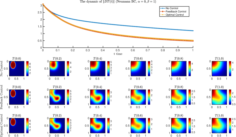
Figure 1: The snapshots of state $T(t)$ at different time points for Example 1 ($t_{f}=1,\tau=0.75$,$\alpha=0,\beta=1$).

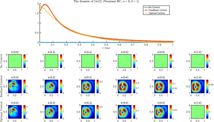
Figure 2: The snapshots of control $\mathbf{v}(t)$ at different time points for Example 1 ($t_{f}=1,\tau=0.75$,$\alpha=0,\beta=1$).

4.2 Example 2

The second example considers the smooth initial condition with two oval-shaped bumps defined by

$$T_{0}(x,y) =10\left(0.5+\frac{1}{\pi}\arctan\left(10(1-32(x-0.25)^{2}-16(y-0.25)^{2})\right)\right)$$

$$+10\left(0.5+\frac{1}{\pi}\arctan\left(10(1-32(x-0.75)^{2}-16(y-0.25)^{2})\right)\right),$$

where the two heated regions are located within two ellipses centered at $(0.25,0.25)$ and $(0.75,0.25)$. Table 2 reports the attained different objective functionals and control measurements. Figures 3–4 present the decay of $\|DT(t)\|$ and $\|\mathbf{v}(t)\|$ and the snapshots of temperature distribution and control velocity field at different time points, respectively. Similar to Example 1, the feedback control (with the choice $\tau=0.75$) and optimal control provide about 26.2% and 29.4% reduction, respectively, in the objective functionals compared to the case with no control. However, Figure 3 demonstrates that different controls may lead to very different evolution of temperature distribution.

Table 2: Control performance comparison of Example 2 with Neumann BC ($\alpha=0,\beta=1,\gamma=0.025$)

Control	$(N_{x},N_{y},N_{t})$	$J(\mathbf{v})$	$J_{\beta}$	$J_{\gamma}$	$\VERT\nabla\cdot\mathbf{v}\VERT_{\infty}$	$\VERT\mathbf{v}\VERT_{\infty}$	Iter	CPU
None ($\mathbf{v}=0$)	(160,160,160)	2.296	2.296	0.000	0.000	0.00	–	13.2
Optimal	(160,160,160)	1.622	1.163	0.460	0.013	1.95	14	528.6
Feedback ($\tau=0.25$)	(160,160,160)	2.030	1.990	0.040	0.013	0.61	–	223.3
Feedback (${\tau=0.5}$)	(160,160,160)	1.766	1.557	0.209	0.017	1.32	–	223.5
Feedback ($\tau=0.75$)	(160,160,160)	1.695	1.269	0.427	0.020	1.93	–	225.4
Feedback ($\tau=1.0$)	(160,160,160)	1.730	1.091	0.638	0.023	2.46	–	224.5

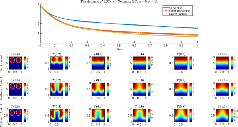
Figure 3: The snapshots of state $T(t)$ at different time points for Example 2 ($t_{f}=1,\tau=0.75$,$\alpha=0,\beta=1$).

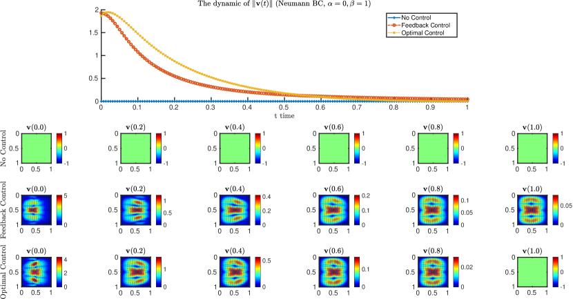
Figure 4: The snapshots of control $\mathbf{v}(t)$ at different time points for Example 2 ($t_{f}=1,\tau=0.75$,$\alpha=0,\beta=1$).

4.3 Example 3

For the sake of numerical test, the third example examines the initial condition with two squared bumps given by

$$T_{0}(x,y)=10\times\mathds{1}_{S},$$

with $S=[0,0.5)^{2}\cup(0.5,1]^{2}$ and $\mathds{1}$ denotes the indicator function. In this case, the initial condition $T_{0}$ is indeed discontinuous, but it will be quickly smoothed out due to diffusion. Table 3 reports the attained different objective functionals and control measurements. Figures 5–6 present the decay of $\|DT(t)\|$ and $\|\mathbf{v}(t)\|$ and the snapshots of temperature distribution and control velocity field at different time points, respectively. Compared with no control, the optimal control provides 22.8% reduction in $J(\mathbf{v})$, while the feedback control (with $\tau=1$) attains only 7.7% reduction in $J(\mathbf{v})$. The controlled dynamics demonstrate quite different pattern during the early stage. Again, the computation of optimal control costs about three times longer CPU time than the feedback control. This example shows that the sub-optimal feedback control may be far away from being optimal. Similar results can be obtained with the corresponding smoothed initial condition (e.g. use smooth rounded squares as heated source).

Table 3: Control performance comparison of Example 3 with Neumann BC ($\alpha=0,\beta=1,\gamma=0.025$)

Control	$(N_{x},N_{y},N_{t})$	$J(\mathbf{v})$	$J_{\beta}$	$J_{\gamma}$	$\VERT\nabla\cdot\mathbf{v}\VERT_{\infty}$	$\VERT\mathbf{v}\VERT_{\infty}$	Iter	CPU
None ($\mathbf{v}=0$)	(160,160,160)	3.950	3.950	0.000	0.000	0.00	–	12.8
Optimal	(160,160,160)	3.049	2.144	0.905	0.019	2.41	19	741.3
Feedback ($\tau=0.25$)	(160,160,160)	3.942	3.941	0.002	0.000	0.07	–	231.2
Feedback ($\tau=0.5$)	(160,160,160)	3.919	3.901	0.018	0.001	0.17	–	229.6
Feedback ($\tau=0.75$)	(160,160,160)	3.805	3.602	0.203	0.002	0.66	–	230.0
Feedback ($\tau=1.0$)	(160,160,160)	3.647	3.090	0.557	0.004	1.38	–	230.0
Feedback ($\tau=1.25$)	(160,160,160)	3.599	2.750	0.849	0.007	1.99	–	228.5
Feedback ($\tau=1.5$)	(160,160,160)	3.617	2.536	1.081	0.009	2.47	–	228.6
Feedback ($\tau=1.75$)	(160,160,160)	3.660	2.391	1.269	0.011	2.87	–	228.7

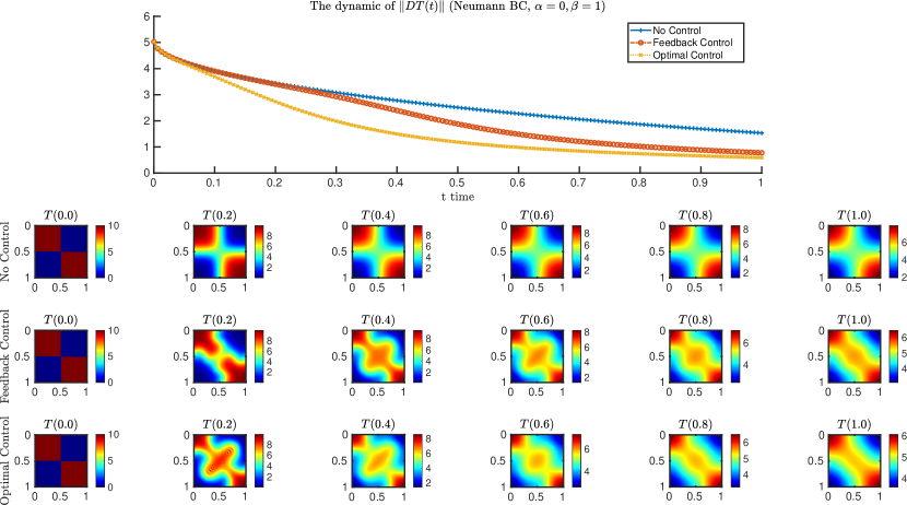
Figure 5: The snapshots of state $T(t)$ at different time points for Example 3 ($t_{f}=1,\tau=1$,$\alpha=0,\beta=1$).

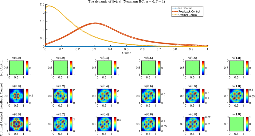
Figure 6: The snapshots of control $\mathbf{v}(t)$ at different time points for Example 3 ($t_{f}=1,\tau=1$,$\alpha=0,\beta=1$).

To illustrate how the performance of feedback control depends on the key parameter $\tau\geq 0$, we plot in Figure 7 the values of $J(\mathbf{v})$ as a function of $\tau\in[0,2]$. It shows the best choice of $\tau$ lies in the open interval $(1.2,1.4)$. This can also be seen from the last three rows in Table 3, where the feedback control with $\tau=1.25$ provides a slightly smaller $J(\mathbf{v})$ than with $\tau=1.0$. Based on the previous examples, the best value of $\tau>0$ seems to be problem dependent, which may not necessarily be less than $t_{f}=1$, although it was originated as a step size.

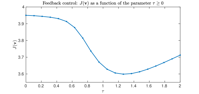
Figure 7: Feedback control: the value of $J(\mathbf{v})$ as a function of the parameter $\tau\in[0,2]$ for Example 3 ($t_{f}=1$,$\alpha=0,\beta=1$).

5 Conclusions

In the current work, we have discussed both optimal and feedback controls for convection-cooling via incompressible fluid flows. First and second necessary optimality conditions were derived for solving and characterizing the optimal control. Motivated by the method of instantaneous control, we investigated the idea of directly constructing the feedback laws by making use of the optimality conditions together with numerical discretization schemes. Our numerical experiments demonstrated the effectiveness of the different control designs. In particular, the sub-optimal feedback control demonstrates comparable performances as the optimal control in some cases. However, there is no rigorous proof for justifying the optimality of the feedback law. Understanding how exactly the mechanism of the nonlinear feedback law plays in the enhancement of convection-cooling or homogenization of a general scalar field, especially, its relation to the diffusivity $\kappa$, the parameter $\tau$ as well as the control weight $\gamma$, requires a more in-depth analysis. The aforementioned issues will be investigated in our future work.

Appendix

Proof of Corollary 2.5.

Proof.

First, with the help of Lemma 2.3, (2.26), and the optimality condition (2.24) we have

$$\int^{t_{f}}_{0}\|\mathbf{v}\|^{2}_{H^{2}}\,dt\leq C\int^{t_{f}}_{0}\|q\nabla T\|^{2}_{L^{2}}\,dt\leq C\sup_{t\in[0,t_{f}]}\|q\|^{2}_{L^{\infty}}\int^{t_{f}}_{0}\|\nabla T\|^{2}_{L^{2}}\,dt\leq C(T_{0},t_{f}).$$ (5.1)

Moreover, by (2.14) and (5.1) we have

$$\sup_{t\in[0,t_{f}]}\|\mathbf{v}\|_{H^{2}}\leq C\sup_{t\in[0,t_{f}]}\|q\nabla T\|_{L^{2}}\leq C\sup_{t\in[0,t_{f}]}\|q\|_{L^{\infty}}\sup_{t\in[0,t_{f}]}\|\nabla T\|_{L^{2}}\leq C(T_{0},t_{f}).$$ (5.2)

To obtain a higher regularity of $T$, we take the inner product of (2.19) with $(-\Delta)^{2}T$ and get

$$\frac{1}{2}\frac{d\|\Delta T\|^{2}_{L^{2}}}{dt}+\kappa\|\nabla(-\Delta T)\|^{2}_{L^{2}}=-(\mathbf{v}\cdot\nabla T,(-\Delta)^{2}T)=(\nabla(\mathbf{v}\cdot\nabla T),\nabla((-\Delta)T))$$

$$\qquad\quad\leq C\|\nabla(\mathbf{v}\cdot\nabla T)\|_{L^{2}}\|\nabla((-\Delta)T\|_{L^{2}}\leq C(\|\nabla\mathbf{v}\cdot\nabla T\|_{L^{2}}+\|\mathbf{v}\cdot\nabla(\nabla T)\|_{L^{2}})\|\nabla((-\Delta)T\|_{L^{2}}$$

$$\qquad\quad\leq C(\|\nabla\mathbf{v}\|^{2}_{H^{1}}\|\Delta T\|^{2}_{L^{2}}+\|\mathbf{v}\|^{2}_{L^{\infty}}\|\Delta T\|^{2}_{L^{2}})+\frac{\kappa}{2}\|\nabla((-\Delta)T\|^{2}_{L^{2}}.$$

This follows

$$\frac{d\|\Delta T\|^{2}_{L^{2}}}{dt}+\kappa\|\nabla((-\Delta)T\|^{2}_{L^{2}}\leq C(\|\nabla\mathbf{v}\|^{2}_{H^{1}}+\|\mathbf{v}\|^{2}_{L^{\infty}})\|\Delta T\|^{2}_{L^{2}}\leq C\|\mathbf{v}\|^{2}_{H^{2}}\|\Delta T\|^{2}_{L^{2}},$$ (5.3)

where we used Among’s inequality (3.32) in the last inequality. Therefore, applying (5.1) to (5.3) yields

$$\sup_{t\in[0,t_{f}]}\|\Delta T\|_{L^{2}}\leq e^{C\int^{t_{f}}_{0}\|\mathbf{v}\|^{2}_{H^{2}}\,dt}\|\Delta T_{0}\|_{L^{2}}<\infty$$ (5.4)

and

$$\kappa\int^{t_{f}}_{0}\|\nabla((-\Delta)T\|^{2}_{L^{2}}\,dt\leq C\int^{t_{f}}_{0}\|\mathbf{v}\|^{2}_{H^{2}}\|\Delta T\|^{2}_{L^{2}}\,dt<\infty.$$ (5.5)

This completes the proof. ∎

Proof of Theorem 2.6.

Proof.

Let $h_{i}\in U_{\text{ad}}$ and $z_{i}=T^{\prime}(\mathbf{v})\cdot h_{i},i=1,2$. Then we have

$$\begin{split}&\frac{\partial z_{i}}{\partial t}=\kappa\Delta z_{i}-\mathbf{v}\cdot\nabla z_{i}-h_{i}\cdot\nabla T,\quad\frac{\partial z_{i}}{\partial n}|_{\Gamma}=0,\\ &z(x,0)=0.\end{split}$$ (5.6)

In light of Corollary 2.5, we can also obtain a higher regularity of $z_{i},i=1,2,$ than (2.18). To see this, taking the inner produce of (5.6) with $-\Delta z_{i}$ follows

$$\frac{1}{2}\frac{d\|\nabla z_{i}\|^{2}_{L^{2}}}{dt}+\kappa\|\Delta z_{i}\|^{2}_{L^{2}}\leq\|\mathbf{v}\|_{L^{\infty}}\|\nabla z_{i}\|_{L^{2}}\|\Delta z_{i}\|_{L^{2}}+\|h_{i}\|_{L^{4}}\|\nabla T\|_{L^{4}}\|\Delta z_{i}\|_{L^{2}}$$

$$\qquad\leq C\|\mathbf{v}\|^{2}_{L^{\infty}}\|\nabla z_{i}\|^{2}_{L^{2}}+C\|\nabla h_{i}\|^{2}_{L^{2}}\|\Delta T\|^{2}_{L^{2}}+\frac{\kappa}{2}\|\Delta z_{i}\|_{L^{2}}.$$ (5.7)

Thus

$$\frac{d\|\nabla z_{i}\|^{2}_{L^{2}}}{dt}+\kappa\|\Delta z_{i}\|^{2}_{L^{2}}\leq C\|\mathbf{v}\|^{2}_{L^{\infty}}\|\nabla z_{i}\|^{2}_{L^{2}}+C\|\nabla h_{i}\|^{2}_{L^{2}}\|\Delta T\|^{2}_{L^{2}},$$

where by (5.4),

$$\int^{t_{f}}_{0}\|\nabla h_{i}\|^{2}_{L^{2}}\|\Delta T\|^{2}_{L^{2}}\,dt\leq\sup_{t\in[0,t_{f}]}\|\Delta T\|^{2}_{L^{2}}\int^{t_{f}}_{0}\|\nabla h_{i}\|^{2}_{L^{2}}\,dt\leq C(T_{0},t_{f})\|h_{i}\|^{2}_{U_{\text{ad}}}.$$

Consequently,

$$\sup_{t\in[0,t_{f}]}\|\nabla z_{i}\|^{2}_{L^{2}}\leq\int^{t_{f}}_{0}e^{C\int^{t_{f}}_{\tau}\|\mathbf{v}\|^{2}_{L^{\infty}}\,ds}\|\nabla h_{i}\|^{2}_{L^{2}}\|\Delta T\|^{2}_{L^{2}}\,d\tau\leq C(T_{0},t_{f})\|h_{i}\|^{2}_{U_{\text{ad}}}$$ (5.8)

and

$$\kappa\int^{t_{f}}_{0}\|\Delta z_{i}\|^{2}_{L^{2}}\leq C\int^{t_{f}}_{0}(\|\mathbf{v}\|^{2}_{L^{\infty}}\|\nabla z_{i}\|^{2}_{L^{2}}+\|\nabla h_{i}\|^{2}_{L^{2}}\|\Delta T\|^{2}_{L^{2}})\,dt\leq C(T_{0},t_{f})\|h\|^{2}_{U_{\text{ad}}}.$$

Next, let $Z=z^{\prime}_{1}(\mathbf{v})\cdot h_{2}$. Then $Z$ satisfies

$$\frac{\partial Z}{\partial t}=\kappa\Delta Z-h_{2}\cdot\nabla z_{1}-\mathbf{v}\cdot\nabla Z-h_{1}\cdot\nabla z_{2},\quad Z|_{\Gamma}=0,$$ (5.9)

$$Z(x,0)=0.$$

Applying an $L^{2}$-estimate for $Z$ gives

$$\frac{1}{2}\frac{d\|Z\|^{2}_{L^{2}}}{dt}+\kappa\|\nabla Z\|^{2}_{L^{2}}\leq\|\nabla h_{2}\|_{L^{2}}\|\nabla z_{1}\|_{L^{2}}\|\nabla Z\|_{L^{2}}+\|\nabla h_{1}\|_{L^{2}}\|\nabla z_{2}\|_{L^{2}}\|\nabla Z\|_{L^{2}}$$

$$\qquad\leq\|\nabla h_{2}\|^{2}_{L^{2}}\|\nabla z_{1}\|^{2}_{L^{2}}+\frac{\kappa}{4}\|\nabla Z\|^{2}_{L^{2}}+\|\nabla h_{1}\|^{2}_{L^{2}}\|\nabla z_{2}\|^{2}_{L^{2}}+\frac{\kappa}{4}\|\nabla Z\|^{2}_{L^{2}},$$

which, together with (5.8), follows

$$\frac{d\|Z\|^{2}_{L^{2}}}{dt}+\kappa\|\nabla Z\|^{2}_{L^{2}}\leq C(\|\nabla h_{2}\|^{2}_{L^{2}}\|\nabla z_{1}\|^{2}_{L^{2}}+\|\nabla h_{1}\|^{2}_{L^{2}}\|\nabla z_{2}\|^{2}_{L^{2}})$$

$$\qquad\leq C(T_{0},t_{f})(\|\nabla h_{2}\|^{2}_{L^{2}}\|h_{1}\|^{2}_{U_{\text{ad}}}+\|\nabla h_{1}\|^{2}_{L^{2}}\|h_{2}\|^{2}_{U_{\text{ad}}}).$$

Therefore,

$$\|Z\|^{2}_{L^{2}}+\kappa\int^{t}_{0}\|\nabla Z\|^{2}_{L^{2}}\,dt\leq C(T_{0},t_{f})\|h_{1}\|^{2}_{U_{\text{ad}}}\|h_{2}\|^{2}_{U_{\text{ad}}},\quad t\in[0,t_{f}].$$ (5.10)

By Lemma 2.2, (2.18) and (5.10), it can be easily verified that the terms on the right hand side of (5.9) are all in $L^{1}(0,t_{f};(H^{1}(\Omega))^{\prime})$, and hence $\frac{\partial Z}{\partial t}\in L^{1}(0,t_{f};(H^{1}(\Omega))^{\prime})$. Thus there exists a unique solution to (5.9), which implies that $T(\mathbf{v})$ is twice G$\hat{a}$teaux differentiable at $\mathbf{v}\in U_{\text{ad}}$ satisfying the optimality condition (2.21), with respect to $h_{1}$ and $h_{2}$, so is $J(\mathbf{v})$.

Now differentiating $J^{\prime}(\mathbf{v})\cdot h_{1}$ once again in the direction $h_{2}\in U_{\text{ad}}$ gives

$$J^{\prime\prime}(\mathbf{v})\cdot(h_{1},h_{2})= \alpha(D^{*}Dz_{2}(t_{f}),z_{1}(t_{f}))+\alpha(D^{*}DT(t_{f}),Z(t_{f}))+\beta\int^{t_{f}}_{0}(D^{*}Dz_{2},z_{1})\,dt$$

$$+\beta\int^{t_{f}}_{0}(D^{*}DT,Z)\,dt+\gamma\int^{t_{f}}_{0}(Ah_{2},h_{1})\,dt.$$ (5.11)

Next taking the inner product of (5.9) with $q$ and applying (2.3), we get

$$\alpha(D^{*}DT(t_{f}),Z(t_{f}))-\int^{t_{f}}_{0}(Z,\frac{\partial q}{\partial t})\,dt=\kappa\int^{t_{f}}_{0}(Z,\Delta q)\,dt+\int^{t_{f}}_{0}(z_{1},h_{2}\cdot\nabla q)\,dt$$

$$\qquad+\int^{t_{f}}_{0}(Z,\mathbf{v}\cdot\nabla q)\,dt+\int^{t_{f}}_{0}(z_{2},h_{1}\cdot\nabla q)\,dt.$$

With the help of the adjoint equations (2.20), we obtain

$$\alpha(D^{*}DT(t_{f}),Z(t_{f}))+\beta\int^{t_{f}}_{0}(Z,D^{*}DT)\,dt=\int^{t_{f}}_{0}(z_{1},h_{2}\cdot\nabla q)\,dt+\int^{t_{f}}_{0}(z_{2},h_{1}\cdot\nabla q)\,dt.$$

Therefore, (5.11) becomes

$$J^{\prime\prime}(\mathbf{v})\cdot(h_{1},h_{2})= \alpha(D^{*}Dz_{2}(t_{f}),z_{1}(t_{f}))+\beta\int^{t_{f}}_{0}(D^{*}Dz_{2},z_{1})\,dt+\int^{t_{f}}_{0}(z_{1},h_{2}\cdot\nabla q)\,dt$$

$$+\int^{t_{f}}_{0}(z_{2},h_{1}\cdot\nabla q))\,dt+\gamma\int^{t_{f}}_{0}(Ah_{2},h_{1})\,dt.$$

Setting $h_{1}=h_{2}=h$ and $z_{1}=z_{2}=z=T^{\prime}(\mathbf{v})\cdot h$ follows

$$J^{\prime\prime}(\mathbf{v})\cdot(h,h)=\alpha\|Dz(t_{f})\|^{2}_{L^{2}}+\beta\int^{t_{f}}_{0}\|Dz\|^{2}_{L^{2}}\,dt+2\int^{t_{f}}_{0}(z,h\cdot\nabla q)\,dt+\gamma\int^{t_{f}}_{0}\|A^{1/2}h\|^{2}_{L^{2}}\,dt.$$ (5.12)

Furthermore, by (2.1), (2.18), (2.25) and (5.8), we get

$$\|Dz(t_{f})\|^{2}_{L^{2}}\leq\frac{C}{\kappa}\|T_{0}\|^{2}_{L^{\infty}}\|h\|^{2}_{U_{\text{ad}}},$$

$$\int^{t_{f}}_{0}\|Dz\|^{2}_{L^{2}}\,dt\leq C\int^{t_{f}}_{0}\|\nabla z\|^{2}_{L^{2}}\,dt\leq\frac{C}{\kappa^{2}}\|T_{0}\|^{2}_{L^{\infty}}\|h\|^{2}_{U_{\text{ad}}},$$

and

$$\left|\int^{t_{f}}_{0}(z,h\cdot\nabla q)\,dt\right|\leq C\int^{t_{f}}_{0}\|\nabla z\|_{L^{2}}\|\nabla h\|_{L^{2}}\|\nabla q\|_{L^{2}}\,dt$$

$$\qquad\leq C\sup_{t\in[0,t_{f}]}\|\nabla z\|_{L^{2}}(\int^{t_{f}}_{0}\|\nabla h\|^{2}_{L^{2}})^{1/2}(\int^{t_{f}}_{0}\|\nabla q\|^{2}_{L^{2}}\,dt)^{1/2}\leq C(T_{0},t_{f})\|h\|^{2}_{U_{\text{ad}}}.$$

As a result,

$$|J^{\prime\prime}(\mathbf{v})\cdot(h,h)| \leq C(T_{0},t_{f})\left(\frac{\alpha}{\kappa}+\frac{\beta}{\kappa^{2}}\right)\|T_{0}\|^{2}_{L^{\infty}}\|h\|^{2}_{U_{\text{ad}}}+\gamma\|h\|^{2}_{U_{\text{ad}}}=(C(T_{0},t_{f},\kappa,\alpha,\beta)+\gamma)\|h\|^{2}_{U_{\text{ad}}}$$

and

$$J^{\prime\prime}(\mathbf{v})\cdot(h,h)\geq -2\int^{t_{f}}_{0}(z,h\cdot\nabla q)\,dt+\gamma\int^{t_{f}}_{0}\|A^{1/2}h\|^{2}_{L^{2}}\,dt=(\gamma-C(T_{0},t_{f},\kappa,\alpha,\beta))\|h\|^{2}_{U_{\text{ad}}}.$$

Therefore, letting $\gamma$ large enough such that

$$\gamma-C(T_{0},t_{f},\kappa,\alpha,\beta)\geq c_{0}>0,$$ (5.13)

we obtain (2.28). ∎

Remark 5.11.

For $T_{0}\in L^{2}(\Omega)$ and $\mathbf{v}\in L^{2}(0,\infty;,H)$, $\|DT\|_{L^{2}}$ obeys an exponential decay rate in time.

Proof.

Taking the inner product of (1.1) with $D^{*}DT$ and applying Greens’ formula and (2.3), we have

$$\frac{1}{2}\frac{d\|DT\|^{2}_{L^{2}}}{dt} =\kappa(\Delta T,D^{*}DT)-(\mathbf{v}\cdot\nabla T,D^{*}DT)$$

$$=\kappa\langle\frac{\partial T}{\partial n},D^{*}DT\rangle\rangle_{\Gamma}-\kappa(\nabla T,\nabla(D^{*}DT))+(\mathbf{v}T,\nabla(D^{*}DT)).$$ (5.14)

Since $\langle T\rangle$ is a function of $t$ and $D^{*}D=D$, we have $\nabla(D^{*}DT)=\nabla(DT)=\nabla(T-\langle T\rangle)=\nabla T,$ and hence using (2.3) and Stokes formula follows

$$(\mathbf{v}\cdot\nabla T,D^{*}DT)=-(T,\mathbf{v}\cdot\nabla(D^{*}DT))=-(\mathbf{v},T\nabla T)=-\frac{1}{2}(\mathbf{v},\nabla(T^{2}))=0.$$

Therefore, (5.14) becomes

$$\frac{1}{2}\frac{d\|DT\|^{2}_{L^{2}}}{dt}+\kappa\|\nabla(DT)\|^{2}_{L^{2}}=0.$$ (5.15)

Further applying Grönwall’s inequality and Poncaré inequality we derive that

$$\|DT\|^{2}_{L^{2}}\leq e^{-C\kappa t}\|DT_{0}\|^{2}_{L^{2}},$$ (5.16)

which establishes the claim. ∎

References

- [1] V. Barbu and G. Marinoschi, An optimal control approach to the optical flow problem, Systems & Control Letters, 87, pp. 1–9, 2016.
- [2] A. Bejan, Convection heat transfer, 2013. John wiley & sons.
- [3] T. R, Bewley, P. Moin and R. Temam, DNS-based predictive control of turbulence: an optimal benchmark for feedback algorithms, Journal of Fluid Mechanics, 447(2), 179–225, 2001.
- [4] T. L. Bergman, F. P. Incropera, A. S. Lavine, and D. P. DeWitt, Introduction to heat transfer, 2011. John Wiley & Sons.
- [5] J. A. Burns and E. M. Cliff, Numerical methods for optimal control of heat exchangers. in Proceedings 2014 American Control Conference, pp. 1649–1654, 2014.
- [6] J. A. Burns and B. Kramer, Full flux models for optimization and control of heat exchangers, in Proceedings of American Control Conference (ACC), pp.577–582, IEEE, 2015.
- [7] B. Calcagni, F. Marsili, and M. Paroncini, Natural convective heat transfer in square enclosures heated from below, Applied thermal engineering, 25(16), 2522–2531, 2005, Elsevier.
- [8] Y. Chang, S. S. Collis, Active control of turbulent channel flows based on large eddy simulation, Proceedings of the FEDSM99. ASME, 6929, 1–8, 1999.
- [9] G. Chen, G. Fu, J. Singler and Y. Zhang, A Class of Embedded DG Methods for Dirichlet Boundary Control of Convection Diffusion PDEs, Journal of Scientific Computing, pp. 1–26, 2019.
- [10] G. Chen, J. Singler and Y. Zhang, An HDG method for Dirichlet boundary control of convection dominated diffusion PDEs, SIAM Journal on Numerical Analysis, 57(4), pp. 1919–1946, 2019.
- [11] G. Chen, W. Hu, J. Shen, J. Singler, Y. Zhang, and X. Zheng, An HDG method for distributed control of convection diffusion PDEs, Journal of Computational and Applied Mathematics, 343, pp. 643–661, 2018.
- [12] H. Choi, R. Temam, P. Moin and J. Kim, Feedback control for unsteady flow and its application to the stochastic Burgers equation, Journal of Fluid Mechanics, 253, 509–543, 1993.
- [13] H. Choi, Suboptimal control of turbulent flow using control theory, Proceedings of the International Symposium on Mathematical Modelling of Turbulent Flows, Tokyo, Japan, 1995.
- [14] H. Choi, M. Hinze, and K. Kunisch, Instantaneous control of backward-facing step flows, Applied numerical mathematics, 31(2), 133–158, 1999.
- [15] P. Constantin and C. Foias, Navier-stokes equations, University of Chicago Press, 1988.
- [16] P. Constantin, A. Kiselev, L. Ryzhik, and A. Zlatoš, Diffusion and mixing in fluid flow, Annals of Mathematics, 643–674, 2008.
- [17] M. Corcione, Effects of the thermal boundary conditions at the sidewalls upon natural convection in rectangular enclosures heated from below and cooled from above, International Journal of Thermal Sciences, 42(2), 199–208, 2003.
- [18] A. Dalal and M. K. Das, Natural convection in a rectangular cavity heated from below and uniformly cooled from the top and both sides, Numerical Heat Transfer, Part A: Applications, 49(3), 301–322, 2006, Taylor & Francis.
- [19] L. Dede’ and A. Quarteroni, Optimal control and numerical adaptivity for advection–diffusion equations, ESAIM: Mathematical Modelling and Numerical Analysis, 39(5), pp. 1019–1040, 2005.
- [20] L. C. Evans, Partial Differential Equations, Vol. 19 of Graduate studies in mathematics, American Mathematical Soc., 2010.
- [21] C. Foias, O. Manley, R. Rosa, and R. Temam, Navier-Stokes equations and turbulence, vol. 83, 2001, Cambridge University Press.
- [22] C. E. Garcia, D. M. Prett,, and M. Morari, Model predictive control: theory and practice–a survey, Automatica, 25(3), 335–348, 1989.
- [23] G. Mathew, I. Mezić, and L. Petzold, A multiscale measure for mixing, Physica D: Nonlinear Phenomena, 211(1), 23–46, 2005.
- [24] G. Mathew, I. Mezić, S. Grivopoulos, U. Vaidya, and L. Petzold, Optimal control of mixing in Stokes fluid flows, Journal of Fluid Mechanics, 580(1), 261–281, 2007.
- [25] R. Glowinski, Y. Song, X. Yuan and H. Yue, Bilinear optimal control of an advection-reaction-diffusion system, https://arxiv.org/abs/2101.02629.
- [26] W. Gong, W. Hu, M. Mateos, J. Singler, X. Zhang, and Y. Zhang, A new HDG method for Dirichlet boundary control of convection diffusion PDEs II: Low regularity, SIAM Journal on Numerical Analysis, 56(4), pp. 2262–2287, 2018.
- [27] M. Hinze and K. Kunish, Control strategies for fluid flows-optimal versus suboptimal control, In H.G.Bock et al., editor, ENUMATH 97, 351–358, 1997.
- [28] M. Hinze, Optimal and instantaneous control of the instationary Navier-Stokes equations, 2000, Citeseer.
- [29] M. Hinze and K. Kunisch, Three control methods for time-dependent fluid flow, Flow, turbulence and combustion, 65(3), 273–298, 2000.
- [30] M. Hinze and S. Volkwein, Analysis of instantaneous control for the Burgers equation, Nonlinear Analysis, 50(1), 1–26, 2002.
- [31] W. Hu, Enhancement of heat transfer in stokes flows, Proceedings of the 56th IEEE Conference on Decision and Control, pp. 59–63, 2017.
- [32] W. Hu and O. San, Optimal Control of Heat Transfer in Unsteady Stokes Flows, 2018 IEEE Conference on Decision and Control (CDC), pp. 3752–3757, 2018.
- [33] W. Hu, Boundary control for optimal mixing by Stokes flows, Applied Mathematics & Optimization 78 (2018), no. 1, 201–217.
- [34] W. Hu and J. Wu, Boundary Control for Optimal Mixing via Navier-Stokes Flows, SIAM Journal on Control and Optimization, 56(4), pp. 2768–2801, 2018.
- [35] W. Hu, An approximating control design for optimal mixing by Stokes flows, Applied Mathematics & Optimization, 82, 471–498, 2020.
- [36] W. Hu and J. Wu, An approximating approach for boundary control of optimal mixing via Navier-Stokes flows, Journal of Differential Equations, 267(10), 5809–5850, 2019.
- [37] C. He, W. Hu, and L. Mu, Optimal control of Convection-cooling and numerical implementation, to appear in Computers & Mathematics with Applications.
- [38] K. Kunisch and X. Lu, Optimal control for multi-phase fluid Stokes problems, Nonlinear Analysis: Theory, Methods & Applications, 74(2), 585–599, 2011.
- [39] F. Kreith, R. M. Manglik, and M. S. Bohn, Principles of heat transfer, 2012. Cengage learning.
- [40] C. Lee, J. Kim and H. Choi, Suboptimal control of turbulent channel flow for drag reduction, Journal of Fluid Mechanics, 358, 245–258, 1998.
- [41] J.-L. Lions, Optimal control of systems governed by partial differential equations, Springer Verlag, 1971.
- [42] Z. Lin, J.-L. Thiffeault, C. R. Doering, Optimal stirring strategies for passive scalar mixing, Journal of Fluid Mechanics, 675, 465–476, 2011.
- [43] E. Lunasin, Z. Lin, A. Novikov, A. Mazzucato, and C.R. Doering, Optimal mixing and optimal stirring for fixed energy, fixed power, or fixed palenstrophy flows, Journal of mathematical physics, 53(11), 115611, 2012.
- [44] W. Liu, Mixing enhancement by optimal flow advection, SIAM journal on control and optimization, 47(2), 624–638, 2008.
- [45] C. Min and H. Choi, Suboptimal feedback control of vortex shedding at low Reynolds numbers, Journal of Fluid Mechanics, 401, 123–156, 1999.
- [46] V. Nevistic and J. A. Primbs, Finite receding horizon control: A general framework for stability and performance analysis, preprint, 1997.
- [47] J. B. Rawlings and K. R. Muske, The stability of constrained receding horizon control, IEEE transactions on automatic control, 38(10), 1512–1516, 1993.
- [48] I. Sezai and A. A. Mohamad, Natural convection in a rectangular cavity heated from below and cooled from top as well as the sides, Physics of Fluids, 12(2), 432–443, 2000, American Institute of Physics.
- [49] G. Stampacchia, Le problème de Dirichlet pour les équations elliptiques du second ordre à coefficients discontinus, Annales de l’institut Fourier, 15(1), 189–257, 1965.
- [50] R. Temam, Navier–Stokes equations and nonlinear functional analysis, SIAM 1995.
- [51] R. Temam, Navier-Stokes Equations, Theory and Numerical Analysis, Studies in Mathematics and Its Applications, Vol. 2, North-Holland.
- [52] J.-L. Thiffeault, Using multiscale norms to quantify mixing and transport, Nonlinearity, 25(2), R1, 2012.
- [53] A. Unger and F. Tröltzsch, Fast solution of optimal control problems in the selective cooling of steel, ZAMM-Journal of Applied Mathematics and Mechanics/Zeitschrift für Angewandte Mathematik und Mechanik: Applied Mathematics and Mechanics, 81(7), 447–456, 2001.
- [54] Walker HF, Ni P. Anderson acceleration for fixed-point iterations. SIAM Journal on Numerical Analysis. 2011;49(4):1715-35.