The yielding of amorphous solids at finite temperatures

Abstract

We analyze the effect of temperature on the yielding transition of amorphous solids using different coarse-grained model approaches. On one hand we use an elasto-plastic model, with temperature introduced in the form of an Arrhenius activation law over energy barriers. On the other hand, we implement a Hamiltonian model with a relaxational dynamics, where temperature is introduced in the form of a Langevin stochastic force. In both cases, temperature transforms the sharp transition of the athermal case in a smooth crossover. We show that this thermally smoothed transition follows a simple scaling form that can be fully explained using a one-particle system driven in a potential under the combined action of a mechanical and a thermal noise, namely the stochastically-driven Prandtl-Tomlinson model. Our work harmonizes the results of simple models for amorphous solids with the phenomenological $\sim T^{2/3}$ law proposed by Johnson and Samwer [Phys. Rev. Lett. 95, 195501 (2005)] in the framework of experimental metallic glasses yield observations, and extend it to a generic case. Finally, our results strengthen the interpretation of the yielding transition as an effective mean-field phenomenon.

I Introduction

Amorphous materials are neither perfect solids nor simple liquids. Foams and emulsions, colloidal glasses, oxide and metallic glasses, glassy polymers and some granular media preserve at rest a solid structure, but will flow if a sufficiently large load is applied to them. Accordingly, in the rheology of complex fluids [1] they are often referred to as “yield-stress materials”. The transition between the solid-like elastic response and the irreversible plastic deformation is known as the yielding transition [2]. Statistical physicists have regarded it as a dynamical out-of-equilibrium phase transition, similar to the depinning transition of elastic manifolds in random media [3], and under the light of equilibrium phase transitions theory. Notably, the bulk of recent theoretical work on the yielding transition of amorphous solids has been devoted to the case in which the effect of temperature is disregarded. Both elastoplastic models and molecular dynamic simulations have focused on describing and understanding the athermal deformation and related critical phenomena [4, 5, 2]. Alike the effect of a small external magnetic field in the ferromagnetic-paramagnetic transition of a magnet (say, Ising model), when a finite temperature is taken into account in the deformation of amorphpus solids it is expected to round up the yielding transition, as it does in depinning [6, 7].

When the elementary constituents of the material are large enough ($\gtrsim 1\mu m$) to neglect Brownian motion effects, an athermal approach is well justified and can be even quantitatively predictive (e.g., in dense granular suspensions, dry granular packings, foams, and emulsions) . Yet, thermal fluctuations may play a role in materials with small enough ($\lesssim 1\mu m$) elementary constituents, e.g., colloidal and polymeric glasses, colloidal gels, silicate and metallic glasses. For those materials, thermally activated events cannot be immediately disregarded. It happens typically though, that driven systems respond on much shorter times than quiescent aging systems; and then, some thermal materials may be treated as athermal for all practical purposes when considering mechanical deformation. Nevertheless, the most interesting physical behavior emerges when the thermal agitation and driving time scales compete, either because temperature is high enough or because the driving is slow. The yielding transition, the limit of vanishing strain rate itself, is of course within this scope.

In a famous paper [9] Johnson and Samwer (J&S) analysed the behavior of a broad range of metallic glasses, finding a universal temperature correction to the compressive yield strength scaling as $\sim T^{\frac{2}{3}}$:

$$\tau_{cT}=\tau_{c0}\left(1-[AT\ln(\omega_{0}/C\dot{\gamma})]^{\frac{2}{3}}\right)$$ (1)

where $\tau_{cT}$ is the compression stress at yielding at temperature $T$, and $\tau_{c0}$ the corresponding value at $T=0$. This law was derived by estimating the transition rate over typical energy barriers in a Frenkel-like construction for the elastic energy of shear transformation zones [9], using an attempt frequency $\omega_{0}$, and a typical height of barriers that decreases as the applied stress is increased, vanishing as a $\frac{3}{2}$ power of the stress remaining to reach instability .

The J&S $\sim T^{\frac{2}{3}}$ law was recovered by MD simulations of 2D Lennard-Jones glasses in Ref. [11]. This time, not just the stress at yield but the full flow/curve was tested for thermal effects and compared with the athermal case. In that numerical work, the following law was proposed and shown to hold for the steady-state stress $\sigma$ as a function of $T$ at a stationary value of $\dot{\gamma}$

$$\sigma(\dot{\gamma},T)=\sigma_{c}+A_{1}\sqrt{\dot{\gamma}}-A_{2}T^{\frac{2}{3}}[\ln(A_{3}T^{\frac{5}{6}}/\dot{\gamma})]^{\frac{2}{3}}.$$ (2)

Finally, a refinement of the theoretical derivation for the $\sim T^{\frac{2}{3}}$ law was proposed in [12], basically following the same principle of Arrhenius-like activation of Eshelby events, with barriers $U_{b}\sim(1-\sigma/\sigma_{c})^{3/2}$. In the present work we will interpret Johnson and Samwer’s $\sim T^{\frac{2}{3}}$ law as a particular case of our derived scaling laws for the thermal rounding of yielding, which are not restricted to a sole kind of energy barriers.

Some endeavors in understanding thermal effects in the deformation of amorphous solids proceeded along the path of analyzing the elementary plastic events and their temperature dependence [13, 14, 15]. But the vast majority of literature devoted to the statistical aspects of the yielding transition (e.g. [4, 16, 17, 18, 5, 19, 20, 21, 22, 23, 24]) has largely ignored the thermal case. Only very recently a preprint by Popovic and co-workers appeared discussing the thermal rounding of the yielding transition [25]. They show that indeed a scaling law for the thermal rounding holds in numerical simulations and prove it analytically for the Hèbraud-Lequeux model. Interestingly, the thermal rounding scaling with roots in mean-field theory of charge-density waves depinning [26, 27] works very well in spatially distributed systems for the description of yielding, essentially with no corrections. While this is somehow good news from the phenomenological point of view (since it simplifies the physical laws to be considered in more applied fields), it contrasts with the yielding theories claiming non-trivial correlations and corrections to scaling in finite dimensions [28, 29].

In this work, we will discuss along these lines, hoping to bring some light to the latter issue. First, we recall the behavior of thermal rounding in a well studied depinning case [30], to show that indeed in short-ranged interaction systems corrections to scaling are expected. After that, we present the possible scenario for thermal rounding of yielding obtained by a generalization of the arguments used in depinning. Then, we present results of numerical simulations on two different coarse-graining frameworks that have been proposed to study the yielding transition. One is the familiar case of elasto-plastic models that have been used to describe yielding for quite a long time already [2]. We introduce temperature in this models as an Arrhenius activation probability over finite energy barriers. The second framework we consider is a Hamiltonian model in which many mean-field like characteristics of yielding have been discussed in recent years [24, 23] Finally, we analyze the results we obtain in both of these extended systems to the light of a one-particle ‘mean-field’-like model, the Prandtl-Tomlinson model of friction [31] with stochastic driving [32]. The thermal rounding behavior of this model also displays  a $\sim T^{\frac{2}{3}}$ phenomenological law analogous to the one proposed by Johnson and Samwer [9].

I.1 The thermal rounding scaling

In standard critical phenomena a symmetry breaking external field transforms a sharp transition into a crossover. For the paradigmatic ferromagnetic-paramagnetic equilibrium phase transition the magnetization ($m$) as a function of temperature ($T$) and magnetic field ($h$) satisfies (sufficiently close to the critical point $T=T_{c}$, $h=0$) the following scaling relation

$$m(T,h)=h^{a}F((T-T_{c})/h^{1/b})$$ (3)

with $F$ a universal scaling function. The critical exponent $a$ quantifies the effect of magnetic field right at $T_{c}$. In the limit of $h\to 0$ this expression must become field-independent, and then, it reduces to the critical form $m\sim(T-T_{c})^{\beta}$ with $\beta=ab$. For the depinning transition of elastic manifolds, a thermal rounding scaling expression was proposed long time ago by Fisher [34, 35] (and numerically tested by Middleton [27]) based on the analogy with equilibrium phase transitions. With the velocity $v$ as the order parameter, the force $f$ as the control parameter and the temperature $T$ as a “symmetry-breaking field” destroying the pinned phase, it has the form

$$v(f,T)=T^{\psi}G((f-f_{c})/T^{1/\alpha}).$$ (4)

As for standard phase transitions, a new exponent $\psi>0$ is introduced, describing the smearing effect, $v\sim T^{\psi}$ at $f=f_{c}$. The form of the scaling function $G$ is such that for $T\to 0$ we re-obtain the expected critical behavior $v\sim(f-f_{c})^{\beta}$ with $\beta=\alpha\psi$ at $T=0$. The driving force in the depinning transition thus plays the role of the temperature in the magnetic system, and temperature the role of external magnetic field. Eq. (4) can be shown to rigorously apply in the fully-connected mean-field problem [34], or equivalently, in the problem of a single particle driven on a disordered potential [36, 37, 38]. Yet, in the more standard situation for the depinning problem, namely short-range elasticity of the manifold in finite dimensions, the precise assessment of the thermal rounding has proved to be non-mean-field and tricky [39]. For instance, the numerically determined value of the $\psi$ exponent varies widely among different models [40, 41, 42, 43, 44, 45, 38]. Furthermore, the scaling form [46] and its universality has been questioned [27]. Even if $\psi$ was a universal exponent, it is not clear whether it is an independent exponent or it is related to other depinning exponents. More recently, general arguments have suggested that Eq. (4) may be not generic, but rather a special case [30], and recent works show that elastic lines in uncorrelated [38] and correlated potentials [30] in finite dimensions display logarithmic corrections that can not be accounted for by the mean-field scaling form.

Athermal amorphous solids undergo a yielding transition well described by the so-called Herschel-Bulkley law relating the deformation rate $\dot{\gamma}$ and the applied stress $\sigma$

$$\sigma=\sigma_{c}+A\dot{\gamma}^{n}$$ (5)

with $n>0$ and $\sigma_{c}$ the critical stress; which sometimes is written as

$$\dot{\gamma}=A^{-1}(\sigma-\sigma_{c})^{\beta}$$ (6)

with $\beta=1/n$. Most yield stress materials in the lab show an exponent $n$ close to 0.5 ($\beta\simeq 2)$, within a relatively broad range of variation [1]. Some of us have recently found that two-dimensional elastoplastic models display exponents $\beta\simeq 3/2$ or $\beta\simeq 2$, according to the local yielding rate for an over-stressed site $i$ being, respectively, constant or stress-dependent (as $\sqrt{\sigma_{i}-{\sigma_{\tt Y}}_{i}}$, with ${\sigma_{\tt Y}}_{i}$ the local instability threshold) [22]. Furthermore, these rules were mapped to the cases of “cuspy” and “smooth” disordered potentials in alternative Hamiltonian models for yielding [24, 22]; that in turn allow to understand the existence of such a $\beta$ exponent dichotomy when comparing them with the problem of a particle stochastically driven in a disordered potential [47], which allows to justify those two values.

Along the lines followed for the depinning transition, the zero temperature flowcurve expression (Eq. 6) can be readily generalized to a proposal for the thermal rounding of the yielding transition

$$\dot{\gamma}(\sigma,T)=T^{\psi}G((\sigma-\sigma_{c})/T^{1/\alpha}).$$ (7)

The form of the scaling function $G$ in Eq. (7) is expected to have, for a large negative argument $x$, a leading term which is exponential in $x^{\alpha}$, reflecting in this limit the thermal activation over barriers that scale as $(\sigma_{c}-\sigma)^{\alpha}$. If we thus use $G(x)=C_{1}\exp(C_{0}(-x)^{\alpha})$ for large negative $x$ in Eq. (7), and invert to obtain $\sigma$, we get

$$\sigma(T)=\sigma_{c}-(C_{0}^{-1}T\log(C_{1}T^{\psi}/\dot{\gamma}))^{1/\alpha}$$ (8)

which can be matched with the Johnson-Samwer expression (up to non-leading terms) if $\alpha$ turns out to be 3/2. We will see in fact that this is the value of $\alpha$ that corresponds in our simulations to the case of smooth potentials, since they generate an energy barrier vanishing as $(\sigma-\sigma_{c})^{3/2}$ as the critical stress is approached.

If Eq. (7) describes correctly the full rounding of the transition, it must also work for positive arguments of the $G$ function, in particular for $T\to 0$. If this is the case, $G(x)$ for large positive $x$ must behave as $\sim x^{\alpha\psi}$ to cancel out the $T$ dependence, showing that the $\psi$ exponent is not independent but is given in terms of the barrier exponent $\alpha$ and the flow exponent $\beta$ as $\psi=\beta/\alpha$. We will show that in fact this holds for $\psi$ both in the case of “cuspy” ($\alpha=2$) and “smooth” ($\alpha=3/2$) potentials, since the kind of underlying disordered potential also determines the flowcurve exponent $\beta$.

Here we not only confirm numerically the good agreement with the scaling predicted by Eq. (7) but also clarify its origin. We also justify the validity of Eq. (7) as is, without the corrections to scaling that are expected in low-dimensional cases with short-range elasticity [30]. Therefore, as we discuss deeper in the following, the finding that for yielding Eq. 7 is indeed very well satisfied can be considered as a manifestation of the mean-field-like nature of the yielding phenomenon.

In the next section we briefly present the two main numerical approaches that we use, namely elastoplastic and Hamiltonian models, leaving a slightly more detailed presentation for Appendix A. Then in Section III we show results in both kind of models, displaying a very robust thermal rounding scaling. In Section IV we interpret those results in terms of the single particle Prandtl-Tomlinson model in the presence of thermal and mechanical noise. Finally, Section VI contains a discussion and summary.

II Models

We run simulations of two different kind of coarse-grained models of amorphous solids: On one hand, ‘Hamiltonian models’ in which disorder is encoded in quenched potentials, the evolution equation of local strains is given by forces derived from a potential and the stochastic process is Markovian. On the other hand, ‘classical EPMs’, where the instantaneous state of elastoplastic blocks constitutes a local ‘memory’ and the system evolution is not necessarily Markovian. In the following we give a minimal description of both frameworks. See Appendix A for a more complete presentation and references to the literature.

II.1 Hamiltonian Model

In the Hamiltonian model we consider the local strain $e({\bf r},t)$, that we will write $e_{i}$ when discretized on a numerical cubic mesh. The temporal evolution of $e_{i}$ is through an overdamped dynamical equation of the form

$$\frac{\partial e_{i}}{\partial t}=-\frac{dV_{i}}{de_{i}}+\sum_{j}G_{ij}e_{j}+\sigma+\sqrt{T}\xi_{i}(t)$$ (9)

Here $\sigma$ is the applied stress, and the strain rate $\dot{\gamma}$ is calculated as

$$\dot{\gamma}\equiv\frac{d\overline{e_{i}}}{dt}=-\overline{\frac{dV_{i}}{de_{i}}}+\sigma$$ (10)

with the bar indicating spatial averaging.

The long range interaction term $G_{ij}$ is of the Eshelby type (see below), and we incorporate temperature through the stochastic term $\xi(t)$ satisfying

$$\langle\xi_{i}(t)\rangle = 0$$ (11)

$$\langle\xi_{i}(t)\xi_{j}(t^{\prime})\rangle = 2\delta(t-t^{\prime})\delta_{ij}.$$ (12)

The potentials $V_{i}$ are disordered potentials, uncorrelated in space, that represent the disordered nature of our amorphous material. We consider two different forms for these potentials, that we call “cuspy” and “smooth”. They are defined in Appendix A1. Both cases describe potentials with many different local minima. The main difference between the two cases is that in the smooth case the force is continuous, whereas in the cuspy case there are discontinuities in the force when moving from one basin to the next.

II.2 Elastoplastic Model

$2$-dimensional elasto-plastic models (EPMs) can be defined by a scalar field $\sigma({\bm{r}},t)$, with ${\bm{r}}$ discretized on a square lattice and each block $\sigma_{i}$ subject to the following evolution in real space

$$\frac{\partial\sigma_{i}(t)}{\partial t}=\mu\dot{\gamma}^{\tt ext}+\sum_{j}G_{ij}n_{j}(t)\frac{\sigma_{j}(t)}{\tau};$$ (13)

where $\dot{\gamma}^{\tt ext}$ is the externally applied strain rate, and the kernel $G_{ij}$ is the Eshelby stress propagator [48]. $G_{ii}<0$ sets the local stress dissipation rate for an active site. The form of $G$ is $G({\bm{r}},{\bm{r}}^{\prime})\equiv G(r,\varphi)\sim\frac{1}{\pi r^{2}}\cos(4\varphi)$ in polar coordinates, where $\varphi\equiv\arccos(({\bm{r}}-{\bm{r}}^{\prime})\cdot{\bm{r}}_{\dot{\gamma}^{\tt(ext)}})$ and $r\equiv\left|{\bm{r}}-{\bm{r}}^{\prime}\right|$. For our simulations we obtain $G_{ij}$ from the values of the propagator in Fourier space $G_{\bf q}$, defined as

$$G_{\bf q}=-\frac{4q_{x}^{2}q_{y}^{2}}{(q_{x}^{2}+q_{y}^{2})^{2}}.$$ (14)

for $\bf q\neq 0$, and $G_{\bf q=0}=-1$.

The elastic shear modulus $\mu=1$ defines the stress unit, and the mechanical relaxation time $\tau=1$, the time unit of the problem. The last term of (13) (for $j\neq i$) constitutes a mechanical noise acting on $\sigma_{i}$ due to the instantaneous integrated plastic activity over all other blocks in the system.

The picture is completed by a dynamical law for the local state variable $n_{i}=\{0,1\}$. Typically a block yields ($n:0\to 1$) when its stress $\sigma_{i}$ reaches a threshold ${\sigma_{\tt Y}}_{i}$ and recovers its elastic state ($n:1\to 0$) after a stochastic time of order $\tau$. The important addition to classic models is that we now allow for thermal activation at finite temperature $T>0$. This is, even when the local stress is below the local threshold $\sigma_{i}<{\sigma_{\tt Y}}_{i}$, the site is activated with probability $\exp(-({\sigma_{\tt Y}}_{i}-\sigma_{i})^{\alpha}/T)$ per unit time. See Appendix A for all the details.

III Results

III.1 Thermal rounding in the Hamiltonian Model

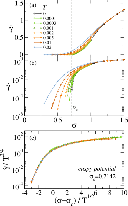
Figure 1: (a) Different temperature flowcurves for a two-dimensional Hamiltonian system of size 512 $\times$ 512, with parabolic potentials. The rightmost curve, $T=0$, fits well a form $\dot{\gamma}\sim(\sigma-\sigma_{c})^{3/2}$ close to $\sigma=\sigma_{c}=0.7142$ (indicated by a vertical dashed line). (b) Same data in log-lin scale. (c) Scaling using $\psi=3/4$, $\alpha=2$ (compatible with $\beta=\psi\alpha=3/2$).

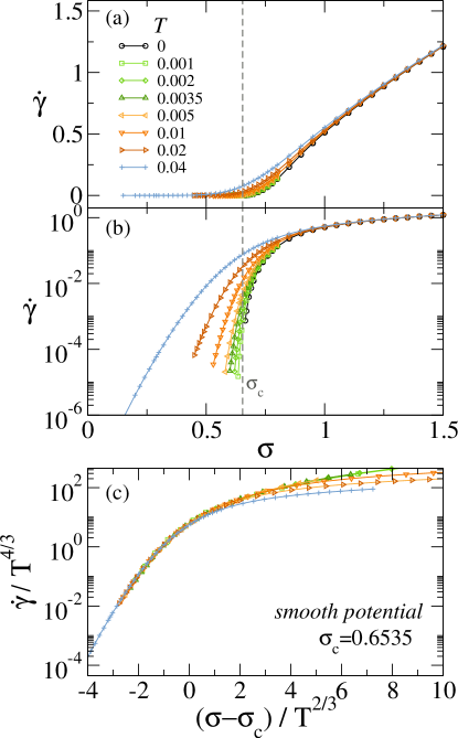
Figure 2: (a) Flowcurves at different temperatures for a two-dimensional Hamiltonian system of size 256 $\times$ 256, with smooth potentials. The rightmost curve, $T=0$, fits well a form $\dot{\gamma}\sim(\sigma-\sigma_{c})^{2}$ close to $\sigma=\sigma_{c}=0.6535$ (indicated by a vertical dashed line). (b) Same data in log-lin scale. (c) Scaling using $\psi=4/3$, $\alpha=3/2$ (compatible with $\beta=\psi\alpha=2$).

We start by presenting the results of our numerical simulations for the Hamiltonian model described in Sec. II.1. In Fig. 1(a) we see the strain rate vs. stress curve (the flow-curve) in a 2D system of size 512$\times$ 512, with disordered potentials formed by concatenation of parabolas which is an instance of the “cuspy” case. The effect of temperature is clearly visible as it generates finite values of strain rates even below the zero temperature critical stress $\sigma_{c}$, that was estimated from a power law fit of the flowcurve corresponding to zero temperature. From the zero temperature fitting we also determine the flow exponent, that to a good approximation turns out to be $\beta=3/2$, as previously reported for this kind of potential [24]. The effect of temperature is more clearly visible plotting the $y$ axis in logarithmic scale (Fig. 1(b)). In this logarithmic plot, it is also clearer the possibility to collapse curves at different temperatures in a single scaled curve. This is done in Fig. 1(c), using the scaling proposed in Eq. (7) with $\alpha=2$ and $\psi=3/4$. The scaling collapse is very good. It extends to a wide range around $\sigma_{c}$ (at least of $\simeq 30\%$ of $\sigma_{c}$), and to temperatures up to $\simeq 0.02$ (to be compared with the reference energy value $\sim 1$ that is the typical height of local barriers when $\sigma=0$).

The rational behind the values of the exponents used in the previous scaling collapse is the following. The value of $\alpha=2$ indicates that the activation barrier for $\sigma$ slightly below $\sigma_{c}$ grows as $(\sigma_{c}-\sigma)^{2}$, which is consistent with the straightforward result obtained in a one-particle system (see Sec. IV), considering the cusps between successive parabolic pieces of the potential in which a particle moves. As we know from previous works [32, 24, 22], the kind of disordered potential will also determine $\beta$. Therefore we say that $\alpha$ and $\beta$ should be ‘compatible’. In fact, if Eq. 7 is to be applicable to the limit $T\to 0$, then the $T$ dependence in this limit must vanish, providing $\psi=\beta/\alpha=3/4$ ($\beta=3/2$ and $\alpha=2$ in this case), which is precisely the value used in Fig. 1(c) to obtain a good collapse of the data.

A similar analysis and scaling can be done for the case of smooth potentials, here constructed by combining sinusoidal functions (see Appendix A). Results (for a system of size $256\times 256$) are shown in Fig. 2. We see that in this case the range of validity of the scaling is somewhat more limited in extent than in the previous case. This is simply a consequence of the fact that the extent of the critical region of the $T=0$ case is smaller . The values of the exponents that are expected to fulfill the scaling are $\beta=2$ and $\alpha=3/2$ (see Sec. IV and [32, 24]). Requiring the exponent $\psi$ to satisfy the relation $\psi=\beta/\alpha$, it results $\psi=4/3$. From the collapse of Fig. 2(c) we conclude that the scaling of Eq. 7 works perfectly well also in the present case of $\beta=2$ and $\alpha=3/2$, thus indicating that the thermal rounding scaling is robust with respect to details of the form of the disordered potential.

III.2 Thermal rounding in elasto-plastic models

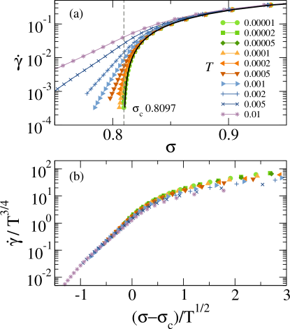
Figure 3: (a) Flowcurves at different temperatures for a two-dimensional EP model of size $2048\times 2048$, with renewable thresholds taken randomly from a distribution and instantaneous plastic events. The barrier coefficient used is $\alpha=2$. The continuous black line corresponds to $T=0$. (b) Scaling (7) using $\psi=3/4$, $\alpha=2$ (compatible with $\beta=\psi\alpha=3/2$).

We now test the thermal rounding scaling of Eq. 7 in different EPMs. First, notice that many classical EPMs (e.g. [48, 18, 5]) consider a common local threshold for all sites and a local stochastic rule to define the precise moment of the local yielding. In the construction of $T>0$ EPMs we have chosen instead to use distributed local thresholds (as in  [50]) and immediate yielding upon reaching the threshold, avoiding an extra stochastic rule for the site activation. Instead, we now include the possibility for a site to be activated by temperature, with a probability $\exp\left[-({\sigma_{\tt Y}}_{i}-\sigma_{i})^{\alpha}/T\right]$ (see Appendix A).

In Fig. 3 we show flowcurves at different temperatures for an EPM with exponentially distributed thresholds (${\sigma_{\tt Y}}_{i}=1+0.1r_{e}$, with $r_{e}$ an exponentially distributed random number) and instantaneous plastic events, i.e., the stress relaxation occurs in a single time step. Panel (a) shows the flowcurves in log-lin scale. Using a $\sigma_{c}=0.8095$ obtained by extrapolating the $T=0$ flowcurve, the expected “universal” exponent $\beta=3/2$ for this kind of EPM , and the corresponding value of $\alpha=2$ used in the activation rule, we observe a good collapse in a wide range of temperatures and strain rates for the scaling (7) with $\psi=\beta/\alpha=3/4$.

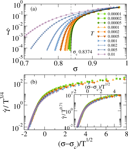
Figure 4: (a) Flowcurves at different temperatures for a two-dimensional EP model of size 2048 $\times$ 2048, with renewable thresholds taken randomly from a distribution and finite duration plastic events. The barrier coefficient used is $\alpha=2$. The continuous black line corresponds to $T=0$. (b) Main plot: scaling (7) using $\psi=3/4$, $\alpha=2$ (compatible with $\beta=\psi\alpha=3/2$) Inset: scaling (7) but with an effective value $\beta=1.42$ used instead, keeping $\alpha=2$ and $\psi=\beta/\alpha$.

If we now add a bit more of phenomenology in the elastoplastic modeling and allow for a ‘finite duration’ of plastic events , we start to loose the formal analogy with the Hamiltonian systems. In particular, the dynamics is now non-Markovian due to the local state memory (see (43)). Yet, we can still test the thermal scaling 7. In fact, flowcurves at $T=0$ for EPMs with finite event duration were seen to recover the $\beta$ exponent prescribed by the Hamiltonian systems and derived from the PT model, but only at small enough strain-rate values and with deviations out of the scaling regime ascribed precisely to the finite duration of the events [22].

Figure 4 shows flowcurves at different temperatures for an EPM with randomly distributed thresholds (${\sigma_{\tt Y}}_{i}=1+0.1r_{e}$, with $r_{e}$ an exponentially distributed random number) and a finite duration for plastic events ($\tau_{\tt off}=1$). We first observe that the finite duration of the events modifies the estimated critical stress $\sigma_{c}$, which is highly non-universal, respect to the one of Fig. 3. The scaling displayed in the main plot of panel (b), using $\psi=3/4$ and $\alpha=2$ is not bad, but also not perfect. In paticular, it is displeasing to see that the curves do not strictly collapse at $\sigma=\sigma_{c}$. Since the true critical region and the existence of universal exponents can be limited to a range of very small strain rates and stresses around the critical point, we checked the possibility of having a better collapse with an effective value of $\beta$ that takes into account the possibility of corrections to the ideal scaling. The inset of Fig. 4(b) uses $\beta\simeq 1.42$ while keeping $\alpha=2$ and $\psi=\beta/\alpha(=0.71)$. This scaling looks better in a wider range of $\dot{\gamma}-\sigma$ values and the scaling assumption (7) perfectly holds. The effective exponent $\beta\simeq 1.42$ is the one that we would fit from the flowcurve at $T=0$ in the range of stresses $[1\times 10^{-4},5\times 10^{-3}]$ above $\sigma_{c}$.

Previous works [32, 24, 22, 23] have indicated that EPMs and the Hamiltonian description are equivalent in some limiting cases. The typical EP modeling (that considers a constant activation probability once a local stress threshold is overpassed) has been seen to correspond to a Hamiltonian model that uses a “cuspy” form for the pinning potential. In order to represent the case of “smooth” potentials EPMs have to use a “progressive” activation law, as described in  [22]. This analogy reflects qualitatively the way in which a block escapes from a local solid state and moves to the next one by local fluidization and the typical time it takes to do so [22]. The matching is further reinforced by the finding that the flow exponent $\beta$ is very close to 3/2 both in Hamiltonian models with cuspy potentials and EPMs with uniform activation, whereas $\beta\simeq 2$ is found in Hamiltonian models with smooth potentials and EPMs with the appropriate progressive activation. Therefore, we believe that once the kind of barrier has been selected (equivalently, the type of local yielding rule), both $\alpha$ and $\beta$ are simultaneously defined, i.e., they are not independent exponents in any physically relevant situation.

Recently Popovic et al. [25] have presented a study of thermal rounding in elastoplastic models, finding a very good scaling of the form of Eq. (7). While they have varied $\alpha$ freely to nicely test the scaling for different kind of thermal activations, the article unfortunately does not discuss in detail the values of $\beta$ (and therefore $\psi$) used for the scaling. Furthermore, there is no discussion on the “curious” fact that the scaling obtained is extremely good, actually more than expected in other cases of thermal rounding of models with non mean-field scaling [30]. Interestingly, one could interpret that such a good mean-field-like scaling is somehow in contrast with previous expectations from the same group about the yielding exponent $\beta$ being non-universal and significantly affected by finite-dimensional effects [29]. We think that the excellent performance of the thermal rounding scaling (7) is not a fortuitous coincidence, but instead a consequence of the fact that the yielding transition is effectively mean-field, as we discuss in the next Section.

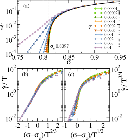
Figure 5: (a) Different temperature flowcurves (in log-lin) for a two-dimensional EP model of size 2048 $\times$ 2048, with thresholds taken randomly from a distribution, renewed after each plastic event, and instantaneous plastic events. The barrier coefficient used is $\alpha=1.5$. The continuous black line corresponds to $T=0$. (b) Scaling (7) using $\psi=1$, $\alpha=3/2$ (compatible with $\beta=\psi\alpha=3/2$). (c) Wrong scaling, using $\psi=3/4$, $\alpha=2$ (compatible with $\beta=\psi\alpha=3/2$).

As a matter of fact, one way to test the mean-field-like hypothesis is to build a system in which we define arbitrarily the kind of activation barrier under consideration. This may lead to an equally arbitrary value of $\psi$. But, as soon as we know that the characteristics that determines $\beta$ is preserved, we can expect the same thermal rounding scaling to hold, with $\psi=\beta/\alpha$.

In Fig. 5 we use an “incorrect” value of alpha in the activation barrier, $\alpha=1.5$, while the plastic events still occurs at a fix rate (as soon as they reach the local threshold). Therefore, with the $\beta=3/2$ expected for constant rates, the scaling (7) translates to $\dot{\gamma}/T$ vs. $(\sigma-\sigma_{c})/T^{2/3}$. This is what is plotted in Fig. 5(b). Despite small deviations to scaling away from $\sigma_{c}$ for the higher temperatures, which are expected, the scaling behaves quite well. Yet, notice that the scaling exponents that worked well in Figs. 3 and 4, i.e., $\dot{\gamma}/T^{3/4}$ vs. $(\sigma-\sigma_{c})/T^{1/2}$, now completely fail, as is shown in (Fig. 5(c)). So, even when we can link $\beta$ at $T=0$ with the type of local yielding rule (constant or progressive when reaching threshold), if we mix that rule with a thermal activation governed by $\alpha$, the scaling relation is still expected to be Eq. 7 with $\psi=\beta/\alpha$. This is why we believe that the scaling works so well for all $\alpha$ in Ref. [25], even when $\beta$ should be similar in all cases, and therefore $\psi$ should be changing.

In brief, we observe that the thermal rounding of Eq. (7) works well in elastoplastic models where the possibility of thermal activation has been introduced in an Arrhenius-like fashion ($\sim\exp(-({\sigma_{\tt Y}}_{i}-\sigma_{i})^{\alpha}/T)$). While the EPMs results alone could leave space for interpretation due to the effective $\beta$ exponents measured, the analogy with the Hamiltonian models strongly suggests that, in the background, the thermal rounding scaling is working with no corrections. This places the yielding phenomenon, beyond the athermal limit, on the spot of a mean-field-like or particle-based theoretical interpretation [22, 23, 53], provided that the non-trivial mechanical noise is well characterized for each dimension. In the next section we combine thermal and mechanical noises in such a one-particle problem.

IV One particle under mechanical and thermal noise

The finding that our numerical results accurately follow the scaling of Eq.(7) with fully consistent values of the exponents provides additional support to a developing idea [24, 32, 22, 23]: The yielding transition in finite dimensions can be accurately described by a mean-field-like model in which a single site feels the effect of all other sites through a “mechanical noise” characterized by a time signal with a non-trivial Hurst exponent $H$ [23]. In Ref.[32] this one-particle model was analyzed in detail at zero temperature, and it was shown that the value of the flow exponent $\beta$ is related to the value of $H$ by

$$\beta=\begin{cases}\frac{1}{H},&\text{``cuspy potential''},\\ \frac{1}{H}+\frac{1}{2},&\text{``smooth potential''}.\end{cases}$$ (15)

where the potentials are periodic and equivalent to the onsite potentials defined for the 2D systems of Sec.II.1 (Eq. (38)),

$$-\frac{dV}{dx}=\begin{cases}[x]-x,&\text{``cuspy''},\\ \sin(2\pi x),&\text{``smooth''}.\end{cases}$$ (16)

Taking into account that $\beta=3/2$ and $\beta=2$ for the cuspy and smooth potentials, respectively, we see that $H$ in the one particle effective model must be taken as [32] $H=2/3$. With this choice, we will show in the following that the addition of an additive thermal noise leads to a good agreement both with the overall form of Eq.(7), and also with the numerical values of the thermal rounding exponents found in the previous sections for the two-dimensional models. Notice that the choice of periodic potentials is done for convenience, since it allows for more straightforward analytic approximations, but the use of bounded disordered potentials keeping the same ‘cuspy’ or ‘smooth’ characteristics would yield identical results.

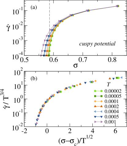
Figure 6: (a) Flow-stress curves for one particle in a cuspy periodic potential composed by concatenated parabolic wells, stochastically driven with mechanical noise of $H=2/3$ at different temperatures. (b) Master curve (Eq.7) using the exponents corresponding to the $\omega=1$ case, $\psi=3/4$ and $1/\alpha=1/2$ from Eq.(24), and $\sigma_{c}=0.5862$.

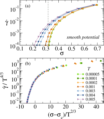
Figure 7: (a) Flow-stress curves for one particle in a sinusoidal potential, stochastically driven with mechanical noise of $H=2/3$ at different temperatures. (a) Master curve (Eq.7) using the exponents corresponding to the $\omega=2$ case, $\psi=4/3$ and $1/\alpha=2/3$ from Eq.(24). $\sigma_{c}=0.319$.

The model that we now simulate consists of a particle with a single coordinate $x$, evolving in a potential $V(x)$, driven by the position variable $w(t)$ through a spring of constant $k_{0}$, and in the presence of a stochastic term that takes into account the effect of temperature $T$ in the system,

$$\frac{dx}{dt}=-\frac{dV}{dx}+k_{0}\left(w(t)-x\right)+\sqrt{T}\eta_{0}(t)$$ (17)

where $\eta_{0}$ is taken as an uncorrelated Gaussian variable such that $\langle\eta_{0}(t)\eta_{0}(t^{\prime})\rangle=2\delta(t-t^{\prime})$. Hence, if $w$ is fixed, the system spontaneously relax to the Boltzmann equilibrium distribution in the potential $V(x)+k_{0}(w-x)^{2}/2$.

The dynamics of the variable $w(t)$ has a smooth part, that mimics the uniform external driving, and a stochastic term that represents the existence of mechanical noise in the system,

$$\frac{dw}{dt}=b\dot{\gamma}+a{\dot{\gamma}}^{H}\eta_{H}(t).$$ (18)

The mechanical noise term is characterized by the Hurst exponent $H$. To implement it, we sample a random variable with a heavy tailed probability distribution,

$$P(\eta_{H})\sim\frac{1}{|\eta_{H}|^{{\frac{1}{H}}+1}},~{}~{}~{}~{}\mbox{for large}~{}~{}|\eta_{H}|.$$ (19)

In practice, we sample it as

$$\eta_{H}=S\left(\frac{1}{R^{H}+\epsilon}-1\right),$$ (20)

where $R$ is a flat random variable between 0 and 1, $S=\pm 1$ is a binary random variable satisfying $\langle S_{t}S_{t^{\prime}}\rangle=\delta(t-t^{\prime})$ and $\langle R_{t}R_{t^{\prime}}\rangle=\delta(t-t^{\prime})/3$, and $\langle S_{t}R_{t^{\prime}}\rangle=0$. Hence, $\eta_{H}$ is also time-decorrelated. It is easy to see that this sampling generates Eq.(19) with a large $\eta_{H}$ cut-off controlled by $\epsilon$.

We have numerically solved the stochastic system of Eqs.(17) and (18) for different values of $T$ and $\dot{\gamma}>0$ in order to obtain the flow-stress ($\dot{\gamma}$ vs $\sigma$) curves near the yielding transition, with the stress $\sigma$ given by the steady-state average

$$\sigma(\dot{\gamma})\equiv k_{0}(\overline{w(t)-x(t)}).$$ (21)

Without loss of generality, in simulations we used the values $k_{0}=0.2$ or $k_{0}=0.5$. These values satisfy the condition $k_{0}<\max_{x}[-V^{\prime\prime}(x)]$ for the cuspy and smooth potentials, thus granting $\sigma(\dot{\gamma}~{}\to~{}0)=\sigma_{c}>0$. We set $\epsilon$ small enough so to assure that scaling exponents are independent of $k_{0}$ and $\epsilon$ [32].

The numerical data for the flowcurves shown in Figs. 6 and 7 show a very good qualitative agreement with the results found for the full 2D system, both for the “cuspy” and “smooth” cases of Eq.(16). In particular, Fig. 6(b) and Fig. 7(b) show a very good scaling collapse when using the expected values $\alpha=2$ and $\beta=3/2$ (and then $\psi=\beta/\alpha=3/4$) for the $\omega=1$ “cuspy” case, and $\alpha=3/2$, $\beta=2$ (and then $\psi=\beta/\alpha=4/3$) for the $\omega=2$ “smooth” case. In fact, it can be analytically shown (see Appendix B) that for low enough temperatures, and sufficiently close to the critical stress $\sigma_{c}$, the flowcurves at different temperatures for the one-particle problem can be cast in the scaled form given by Eq. (7), with the values of the scaling exponents

$$\psi = \frac{\omega-H+\omega H}{(\omega+1)H}$$ (22)

$$\alpha = 1+\frac{1}{\omega}$$ (23)

$$\beta = \psi\alpha=\frac{1}{H}-\frac{1}{\omega}+1$$ (24)

Here $\omega$ is related to the form of the potential $V(x)$ in Eq.(17) right at the transition point between successive wells: $\omega=1$ for the “cuspy”, and $\omega=2$ for the “smooth” potentials defined in Eq.(16) (see Appendix B for a realization of $V$ with a generic $\omega$ and its thermal rounding scaling). It is worth noting from Eq. (24) that the exponents predicted are universal, in the sense that they do not depend on the particular shape of $V(x)$ but only on its normal form near the local yielding thresholds.

V Interpolation between activated and athermal flowcurves. Generalizing the Johnson and Samwer’s law

If in Eq. (8) we set $\dot{\gamma}=\dot{\gamma}_{0}$, where $\dot{\gamma}_{0}$ is such that strain-rates below it are experimentally undetectable, then Eq. (8) can be considered to be a restating of the J&S result, Eq. (1). In other words, the empirical finite-temperature yield stress $\tau_{c,T}$ appearing in Eq.(1) can be identified with the stress evaluated at the threshold strain-rate, $\tau_{c,T}\approx\sigma(\dot{\gamma}_{0},T)<\sigma_{c}$  . More generally, we can propose an interpolation scheme between the exponentially activated regime at $\sigma<\sigma_{c}$ and the zero temperature limiting behavior behavior for $\sigma>\sigma_{c}$ by generalizing Eq. (8) to a form similar to equation (2), namely

$$\sigma(\dot{\gamma},T)=\sigma(\dot{\gamma},T=0)-\left[\frac{T}{C}\ln\left(\frac{C^{\prime}T^{\psi}}{\dot{\gamma}}\right)\right]^{1/\alpha}.$$ (25)

where $\sigma(\dot{\gamma},T=0)$ is expected to behave as

$$\sigma(\dot{\gamma},T=0)=\sigma_{c}+C_{0}\dot{\gamma}^{1/\beta}$$ (26)

In addition to reducing to the standard flowcurve at $T=0$ and to the exponential activation formula when $T\gg\dot{\gamma}^{1/\psi}$, Eqs. (25), (26) are fully compatible with the general thermally activated behavior (Eq. (7)).

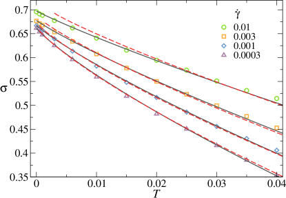
Figure 8: Simulation results for $\sigma$ as a function of $T$ at different $\dot{\gamma}$ levels for the data corresponding to Fig.2. The red-dashed lines correspond to the prediction of Eqs. (25), (26) with $\alpha=3/2$, $\psi=4/3$, $\sigma_{c}=0.6535$, $C_{0}=0.44$, $C=1.70$, $C^{\prime}=27.47$ (notice that this prediction cannot be extended at temperatures lower than $\sim(\dot{\gamma}/C^{\prime})^{1/\psi}$). The gray full lines correspond to the expression (27) with $\alpha=3/2$, $\psi=4/3$, $\sigma_{c}=0.6535$, $C=0.45$, $C^{\prime}=1.41$, $\kappa=0.375$.

It is interesting to check our numerical data against expression (25). For the sake of concreteness we only show the results for the Hamiltonian model in the case of smooth potentials. Using the same parameters that were used to construct Fig. 2, we obtain the red-dashed curves shown in Fig. 8 (notice the analogy with Fig. 2 in [9]). We see that the fitting to the numerical values provided by expression (25) (adjusting constants $C_{0}$, $C$ and $C^{\prime}$ and using the appropriate exponents for this case, namely $\alpha=3/2$ and $\beta=2$) is in fact very good if the temperature is not too small. However in this limit Eq. (25) cannot be correct as the log becomes negative. A full range approximate interpolation scheme can be easily obtained by transforming (25) to

$$\sigma(\dot{\gamma},T)=\sigma(\dot{\gamma},T=0)-\left[\frac{T}{C}\ln\left(C^{\prime}\left(\frac{T^{\psi}}{\dot{\gamma}}\right)^{\kappa}+1\right)\right]^{1/\alpha}.$$ (27)

This regularization of the log is similar to the one that is known to work very well in the Prandtl-Tomlinson model [55], and provides a much better fitting at low $T$ to the data in Fig. 8, as indicated by the gray full lines.

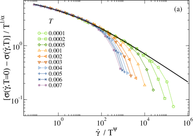
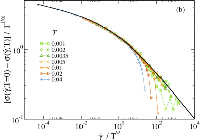
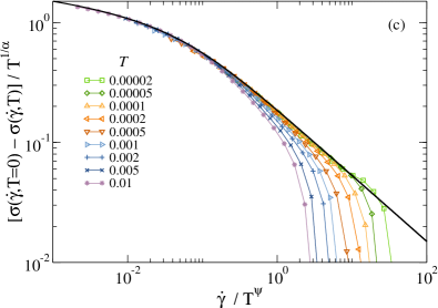
Figure 9: Plot of $[\sigma(\dot{\gamma},T=0)-\sigma(\dot{\gamma},T)]/T^{1/\alpha}$ vs $\dot{\gamma}/T^{\psi}$, for (a) the one particle model and (b) the extended Hamiltonian model (system size 256 $\times$ 256), with smooth potentials ($\psi=4/3$), and for (c) the EP model with instantaneous events (system size 2048 $\times$ 2048), for which $\psi=3/4$. Different temperatures are included and fall into the same mastercurve. In all cases the points are fitted by an expression of the form $y=\left(C^{-1}\log(C^{\prime}/x^{\kappa}+1)\right)^{1/\alpha}$. (one particle: $\alpha=3/2$, $\kappa=0.4$, $C=0.18$, $C^{\prime}=4.5$; Hamiltonian: $\alpha=3/2$, $\kappa=0.5$, $C=0.61$, $C^{\prime}=2$; EPM: $\alpha=2$, $\kappa=1.1$, $C=2.25$, $C^{\prime}=0.08$)

The interpolation scheme of Eq. (27) suggests to plot the values of $y\equiv\left[\sigma(\dot{\gamma},T=0)-\sigma(\dot{\gamma},T)\right]/T^{1/\alpha}$ vs. $x\equiv\dot{\gamma}/T^{\psi}$ for the one-particle and the full extended model to compare in detail the effect of temperature in both cases. In fact, this plot is of the form

$$y=\left[\frac{1}{C}\ln\left(\frac{C^{\prime}}{x^{\kappa}}+1\right)\right]^{1/\alpha}$$ (28)

and must lie on a single master curve if the thermal rounding scaling is satisfied. Results are presented in Fig. 9 for Prandtl-Tomlinson, Hamiltonian and elastoplastic models. We see that the data remarkably collapse on a single master curve as temperature is reduced , and also that in the three cases this curve is accurately fitted by and expression of the form (28). The log-two-thirds behavior (for $\alpha=3/2$) of this expression is the one expected based on the interpolation formula Eq. (25). The power of $x$ and the $+1$ added term inside the log give a much better crossover to the power law decay as $x\to\infty$. In any case, the remarkable result is that the same kind of analytical expression provides a very good fitting of the results for the one particle model and for the full extended model.

VI Summary and Discussion

We have addressed the problem of the thermal rounding of the yielding transition of amorphous materials in a comprehensive theoretical framework, both including different modeling approaches and analytical arguments and targeting the interpretation of important phenomenological laws based on experimental data from a new perspective. In particular, we have considered two different numerical approaches consisting in spatially extended models that describe stress and strain in the system at a coarse-grain level, where the elastic interaction at finite distance is incorporated through the use of the Eshelby quadrupolar kernel. In one case, coined “Hamiltonian”, the full dynamics has the form of an overdamped equation of motion for the local strain. In this case temperature is included in a standard way through the addition of a Langevin stochastic term to the equations of motion. The second case corresponds to the purely phenomenological approach of elasto-plastic models, where the elastoplastic blocks of the system switches between solid and fluidized states according to local rules that take into account their mechanical stability. In this case we include temperature as an Arrhenius-like activation allowing one block to fluidize even when its stress is lower than the local yielding threshold.

Our first main result has been to extend the compatibility between these modeling approaches to the case of finite temperatures. Previous works [24, 22] indicated that at $T=0$ both approaches display the same qualitative behavior at both quasistatic and finite strain rate deformations. In particular, at $T=0$, irrespective of the model particularities and close to the critical stress $\sigma_{c}$, all flowcurves group in only one of two families [24, 22]: the one corresponding to “cuspy” disordered potentials (equiv. uniform yielding rates in EPMs) with $\beta=3/2$ or the one corresponding to “smooth” disordered potentials (equiv. progressive yielding rates in EPMs) with $\beta=2$. For finite temperatures $\dot{\gamma}$ is different from zero even below $\sigma_{c}$ displaying an exponential activation of the form

$$\dot{\gamma}\sim\exp[-C(\sigma_{c}-\sigma)^{\alpha}/T]~{}~{}~{}~{}~{}~{}~{}~{}(\sigma<\sigma_{c})$$ (29)

The value of $\alpha$ encodes details of the quenched stochastic potential in the Hamiltonian case, or the activation rates as a function of stress in the EPMs. The expected $\alpha$ value corresponding to the most realistic case of a smooth quenched potential (in Hamiltonian modeling) is $\alpha=3/2$, and is the one that should be expected in molecular dynamics simulations and experiments.

The second main result of our work is the observation that the flowcurves, in a finite interval around $\sigma_{c}$, and for finite temperatures (at least when $T$ is not “too large”) are very well described by the thermal rounding scaling of Eq. (7). This scaling extends the exponentially activated regime for $\sigma<\sigma_{c}$ to a full interval around $\sigma_{c}$. In fact we conclude that the Johnson and Samwer relation, Eq. (1), can be derived from Eq. (7) and recovered with all the numerical approaches we have implemented. The connection of the thermal rounding scaling proved in this work with the phenomenological results gathered in [9] strongly suggests that our conclusions, besides a pure theoretical interest, are relevant to the study of thermal rounding of real amorphous materials where a flowcurve can be actually measured, for example, in colloidal glasses [1, 57].

The thermal rounding scaling of eq.7 is predicted from models that assume a well defined temperature $T$ entering either through a Langevin noise or through Arrhenius activation at the corresponding coarse grained level for each case. In the case of amorphous materials with mesoscopic constituents (colloidal glasses/gels, emulsions, foams), whether such $T$ should correspond to the bath temperature or a thermodynamically well defined effective temperature of the material [58, 59] (that incorporate non-equilibrium fluctuations) remains an open and interesting question. Nonetheless, the agreement of our model predictions with the Jhonson & Samwer phenomenological scaling strongly suggests that, at least for metallic glasses, the putative effective temperature $T$ must be equal or proportional to the experimentally measured temperature. In addition, any effective temperature playing the role of $T$ in Eq. 7 should have a negligible $\dot{\gamma}$ dependence, otherwise the whole scaling would fail.

We have also shown that the thermal rounding scaling is analytically satisfied in the case of a single particle driven on a disorder quenched potential, under the action of a mechanical and a thermal noise. This concomitance between the thermal rounding behavior of the one-particle model and that of the full extended model, which extends also to the detail of the analytical form of the full $\sigma(\dot{\gamma},T)$ curve, reinforces our view that the spatially distributed simulation outcomes admit a very accurate description in terms of a one-particle system. In the end, this is an additional indication that the yielding transition of amorphous materials in finite dimensions, at least up to the point in which it is captured by the present kind of models, can be described effectively as a mean field transition.

Appendix A Model description

A.1 Hamiltonian Model

The Hamiltonian description of the yielding transition and plastic behavior has been already presented in [47, 60, 24]. We provide here a short description for completeness. It considers the symmetric, linearized elastic strain tensor of the material $\varepsilon_{ij}(r)$ at different positions $r$ in the sample. It assumes a relaxational dynamics that tends to minimize the free energy of the system, in the form

$$\eta\frac{\partial\varepsilon_{ij}}{\partial t}={-}\frac{\delta F(r)}{\delta\varepsilon_{ij}}+\Lambda_{ij}\varepsilon_{ij}+\sigma_{ij}.$$ (30)

Here, $F\equiv\int d^{d}rf(\varepsilon_{ij})$ is the total free energy, obtained by spatial integration of a free energy density $f$. Note that $f$ is local in $\varepsilon_{ij}$. $\Lambda_{ij}$ are Lagrange multipliers that are necessary to fulfill internal constrains among the $\varepsilon_{ij}$, usually referred to as Saint-Venant compatibility conditions [47, 60]. The $\sigma_{ij}$ are externally applied stresses with different symmetries. In the form given by 30, this is already a model that can be applied to concrete calculations in a fully tensorial framework, once the form of $f(\varepsilon_{ij})$ is defined [61]. However, in the case in which the externally applied stress is homogeneous and of definite symmetry, a further approximate transformation can be proposed, as follows. If, for simplicity, we call $\sigma$ the applied external stress, and $e$ the corresponding component of the strain field, we can (under certain conditions [61]) integrate out the remaining components of the $\varepsilon_{ij}$ tensor, and arrive at a scalar model for $e(r)$. Switching now to a notation in which the latin indexes label spatial positions in the sample, this scalar model reads (we take $\eta=1$ from now on)

$$\frac{\partial e_{i}}{\partial t}={-}\frac{\delta F(e)}{\delta e_{i}}+\sum_{j}G_{ij}e_{j}+\sigma.$$ (31)

Note that the original compatibility conditions have transformed in the non-local interaction term mediated by the kernel $G_{ij}$. The detailed derivation shows that $G_{ij}$ is nothing but the Eshelby interaction also used in EPM’s (see next Section). All that remains to define our model is to specify the form of the free energy $F$. First of all, notice that $F$ is a sum of local term over different parts of the sample, i.e,

$$F(e)=\sum_{i}V_{i}(e_{i})$$ (32)

Since we are interested in modeling an amorphous, disordered material $V_{i}(e_{i})$ will be chosen in such a way that it describes the local thresholding behavior of a small piece of the amorphous material under deformation. The functions $V_{i}$ have minima at different values of $e$ representing local equilibrium states. The functions $V_{i}$ are stocastically defined, in an uncorrelated manner for each site $i$.

$$\frac{de_{\bf q}}{dt}=-\sum_{i}V^{\prime}_{i}(e_{i})|_{\bf q}+G_{\bf q}e_{\bf q}$$ (33)

$G_{{\bf q}=0}$ is taken as zero in a stress conserved dynamics. The uniform mode in Eq.(31) is thus directly found from

$$\dot{\gamma}\equiv\frac{d\overline{e_{i}}}{dt}=\overline{-V^{\prime}_{i}(e_{i})}+\sigma$$ (34)

that defines the global strain rate $\dot{\gamma}$. Finally, the last remaining point is related to the incorporation of temperature. In the present model, there is a simple and natural way to incorporate temperature, namely in the form of a stochastic (Langevin) force, added to the right of Eq. 31, that finally reads

$$\frac{\partial e_{i}}{\partial t}=-\frac{dV_{i}}{de_{i}}+\sum_{j}G_{ij}e_{j}+\sigma+\sqrt{T}\xi_{i}(t)$$ (35)

with the stochastic term $\xi(t)$ satisfying

$$\langle\xi_{i}(t)\rangle = 0$$ (36)

$$\langle\xi_{i}(t)\xi_{j}(t^{\prime})\rangle = 2\delta(t-t^{\prime})\delta_{ij}$$ (37)

We numerically simulate Eq. 35 for two particular on-site periodic potentials referred to as “cuspy”and “smooth” potentials. They are constructed as a concatenation of parabolic (cuspy) or sinusoidal (smooth) pieces, in consecutive intervals of the $e$ axis. Each interval is characterized by its left and right border, $e_{l}$, $e_{r}$, in such a way that the force derived from the potential in a particular interval is given in terms of $e_{0}\equiv(e_{l}+e_{r})/2$ and $\Delta\equiv(e_{r}-e_{l})$ by

$$-\frac{dV}{de}=\begin{cases}e_{0}-e,&\text{``cuspy potential''},\\ \frac{\Delta}{2\pi}\sin(2\pi(e_{0}-e)/\Delta),&\text{``smooth potential''},\end{cases}$$ (38)

The value of $\Delta$ for each interval is taken from a flat distribution within the interval $[1,2]$. It is clear from its definition, that the cuspy (smooth) potential has a discontinuous (continuous) force between consecutive intervals of definition.

We integrate the equation of motion using a first order Euler method with a temporal time step $\delta t=0.1$. All results presented correspond to square samples with periodic boundary conditions. The flowcurve is determined starting from the largest values of $\sigma$, and progressively reducing it, while the strain rate is calculated from Eq. 34. In this way we get rid of issues associated to sample preparation that would appear if the smallest $\sigma$ values were simulated first.

A.2 Elasto-plastic model

When referring to elasto-plastic models (EPMs), we consider amorphous materials at a coarse-grained-level description, laying in between the particle-based simulations and the continuum-level description. Full background, context and historical development of EPMs can be found in [2]. The amorphous solid is represented by a coarse-grained scalar stress field $\sigma({\bm{r}},t)$, at spatial position ${\bm{r}}$ and time $t$ under an externally applied shear strain. Space is discretized in blocks. At a given time, each block can be “inactive” or “active” (i.e., yielding). This state is defined by the value of an additional variable: $n({\bm{r}},t)=0$ (inactive), or $n({\bm{r}},t)=1$ (active).

We define our EPM in $2$-dimensions discretized on a square lattice, and each block $\sigma_{i}$ subject to the following evolution in real space

$$\frac{\partial\sigma_{i}(t)}{\partial t}=\mu\dot{\gamma}^{\tt ext}+\sum_{j}G_{ij}n_{j}(t)\frac{\sigma_{j}(t)}{\tau};$$ (39)

where $\dot{\gamma}^{\tt ext}$ is the externally applied strain rate, and the kernel $G_{ij}$ is the Eshelby stress propagator [48].

It is convenient to explicitly separate the $i=j$ term in the previous sum, as

$$\frac{\partial\sigma_{i}(t)}{\partial t}=\mu\dot{\gamma}^{\tt ext}-g_{0}n_{i}(t)\frac{\sigma_{i}(t)}{\tau}+\sum_{j\neq i}G_{ij}n_{j}(t)\frac{\sigma_{j}(t)}{\tau};$$ (40)

where $g_{0}\equiv-G_{ii}>0$ (no sum) sets the local stress dissipation rate for an active site. The form of $G$ is $G({\bm{r}},{\bm{r}}^{\prime})\equiv G(r,\varphi)\sim\frac{1}{\pi r^{2}}\cos(4\varphi)$ in polar coordinates, where $\varphi\equiv\arccos(({\bm{r}}-{\bm{r}}^{\prime})\cdot{\bm{r}}_{\dot{\gamma}^{\tt(ext)}})$ and $r\equiv\left|{\bm{r}}-{\bm{r}}^{\prime}\right|$. For our simulations we obtain $G_{ij}$ from the values of the propagator in Fourier space $G_{\bf q}$, defined as

$$G_{\bf q}=-\frac{4q_{x}^{2}q_{y}^{2}}{(q_{x}^{2}+q_{y}^{2})^{2}}.$$ (41)

for $\bf q\neq 0$ and

$$G_{\bf q=0}=-\kappa$$ (42)

with $\kappa$ a numerical constant set to 1.

The elastic (e.g. shear) modulus $\mu=1$ defines the stress unit, and the mechanical relaxation time $\tau=1$, the time unit of the problem. The last term of (40) constitutes a mechanical noise acting on $\sigma_{i}$ due to the instantaneous integrated plastic activity over all other blocks ($j\neq i$) in the system. The picture is completed by a dynamical law for the local state variable $n_{i}=\{0,1\}$. Here is where the thermal activation for $T>0$ steps in. In the athermal case, when the local stress overcomes a local yield stress, a plastic event occurs (the block becomes “active”) with a given probability, usually constant (see [22] for different alternatives). But when $T>0$ we also expect activation to occur with a finite probability even when $\sigma_{i}<{\sigma_{\tt Y}}_{i}$. The block ceases to be active when a prescribed criterion is met. When the plastic event has a finite duration, a local memory is coded in the system configuration, defining a dynamics that is typically non-Markovian. In this work we have used the following rules for sites activation and deactivation:

$$n_{i}:\begin{cases}0\rightarrow 1&\mbox{instantaneously~{}}\mbox{\quad if \quad}\sigma_{i}\geq{\sigma_{\tt Y}}\\ 0\rightarrow 1&\mbox{with probability per unit time~{}}\\ &\exp(-({\sigma_{\tt Y}}_{i}-\sigma_{i})^{\alpha}/T)\mbox{\quad if \quad}\sigma_{i}<{\sigma_{\tt Y}}\\ 0\leftarrow 1&\mbox{at a rate~{}}\tau_{\tt off}^{-1}\end{cases}$$ (43)

where $\alpha$ and $\tau_{\tt off}$ are parameters and the ${\sigma_{\tt Y}}_{i}$ variables are randomly sorted after each local yield event to be $1+0.1r_{\tt exp}$, with $r_{\tt exp}$ a random number taken from an exponential distribution of average unity. The case of instantaneous stress release corresponds to $\tau_{\tt off}\to\infty$, otherwise we have set $\tau_{\tt off}=1$. As discussed in [22], the case of EPMs with uniform local yield rates (i.e., constant, as in this case) can be directly related to the case of cuspy potentials in the Hamiltonian model. The $\beta$ exponent of the athermal flowcurve results identical in both approaches. We then believe that the choice of the parameter $\alpha$ in the thermal activation rule is not arbitrary but should respect the same analogy among model approaches. Therefore, here we use $\alpha=2$ which is the barrier exponent in a parabolic potential. On the other hand, the case of smooth potentials in the Hamiltionian approach is analogous to the case of progressive local yield rates [22] in EPMs. In that case the block activation is stochastic by definition. We have avoided here to combine the stochasticity of both progressive rates (e.g. $\tau_{\tt on}\sim(\sigma_{i}-\sigma_{i}^{\tt y})^{-1/2}$) and thermal activation, and choose to show only the uniform rate case for simplicity. But such a combination is possible to do and in that case we would use $\alpha=3/2$ as the barrier exponent for the thermal activation in (43).

Appendix B Scaling for a single particle in a potential

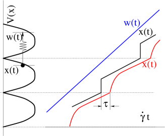
Figure 10: Schematic representation of the dynamics of the Prandtl-Tomlinson model at $T=0$ and $a=0$. On the left, a periodic potential $V(x)$ constructed by a concatenation of parabolas, with a particle moving on it, is depicted with a 90º rotation for visualization. On the right, the driving $w(t)$ and particle position $x(t)$ are shown for $\dot{\gamma}\to 0$ (black) and $\dot{\gamma}>0$ (red). The value of $\sigma$ is obtained as the average of $k_{0}(w(t)-x(t))$. This value is larger when $\dot{\gamma}>0$ than when $\dot{\gamma}\to 0$.

In this appendix we derive the scaling form of the flowcurve for a single particle stochastically driven in a potential in the presence of thermal noise. The stochastic driving is composed of a fix strain-rate, or velocity, plus a mechanical noise characterized by a Hurst exponent $H$. The derivation generalizes the one of Ref. [32] to the case of finite temperatures. The $x$ variable of the system (particle position) follows Eqs.(17) and (18), that we repeat here for convenience

$$\frac{dx}{dt} = -\frac{dV}{dx}+k_{0}\left(w(t)-x\right)+\sqrt{T}\eta_{0}(t)$$ (44)

$$\frac{dw}{dt} = b\dot{\gamma}+a{\dot{\gamma}}^{H}\eta_{H}(t)$$ (45)

The system is driven imposing a constant value of $\dot{\gamma}$. At a given time $t$, $\eta_{H}$ is a random variable sorted as described in Eq. 20. The stress $\sigma$ at any moment is defined as $\sigma\equiv k_{0}(\overline{w(t)-x(t)})$, where $k_{0}$ is a model parameter.

If $T=0$ and $k_{0}<\max_{x}(-V^{\prime\prime}(x))$ there is a finite critical stress value $\sigma_{c}$ when $\dot{\gamma}$ tends to zero. In a general case, for small values of $T$ and $\dot{\gamma}$, $\sigma$ will be close to $\sigma_{c}$ (i.e., $|\sigma-\sigma_{c}|/\sigma_{c}\ll 1$). We want to find a scaling relation between $T$, $\dot{\gamma}$, and $\sigma-\sigma_{c}$ close to the critical point in which all these three variables are vanishing. The idea of the calculation is as follows. Consider the evolution of the variable $x$ as a function of $\dot{\gamma}t$ at $T=0$, $a=0$, and for a vanishingly small $\dot{\gamma}$, as depicted in Fig. 10. As the particle advances in the potential $V(x)$, “jumps” in $x$ occur at the transition points between local basins (black line for $x(t)$ in Fig. 10). The value of the stress is proportional to the average of $w(t)-x(t)$, and in the case of $T=0$ and vanishing $\dot{\gamma}$ will be $\sigma_{c}$.

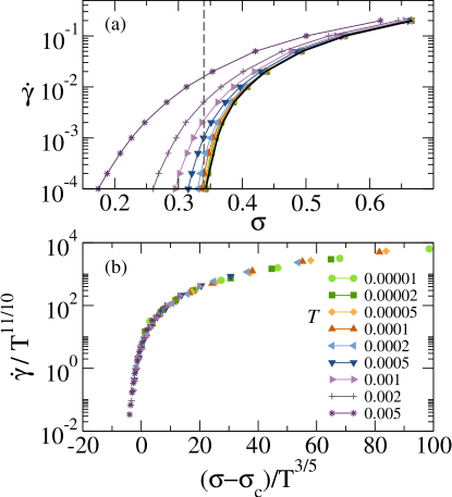
Figure 11: (a) Flow-stress curves for one particle in a periodic potential, with mechanical noise of $H=2/3$ at different temperatures. (b) Master curve (Eq.7) using the exponents corresponding to to the $\omega=3/2$ case, $\psi=11/10$ and $1/\alpha=3/5$ from Eq.(24), and $\sigma_{c}=0.34$.

For finite but small $T$ and $\dot{\gamma}$, the evolution of $x$ will be close but not exactly equal to the previous case. The average of $w(t)-x(t)$ will be different, in particular due to the finite $\dot{\gamma}$, but also due to a finite temperature. The main effect on $\sigma$ can be understood due to a shift in the transition point from one basin to the next one. Now, it is not necessarily true that $x$ will jump exactly when reaching the cusp edge (or the maximum derivative for a smooth potential). We encode this time shift in a variable $\tau$ (see Fig. 10). The change in stress $\delta\sigma\equiv\sigma-\sigma_{c}$ can be estimated as the fraction of time that $\tau$ represents of the total time needed to traverse a basin (a period of the potential). Being the latter $(b\dot{\gamma})^{-1}$, we find $\delta\sigma\sim\tau b\dot{\gamma}$. The following step to quantify the change in $\sigma$ is to obtain the scaling behavior of $\tau$ from Eqs. 44 and 45. Taking into account the importance of the transition points, we first rewrite Eq. 44 close to these points using $-dV(x)/dx\simeq Ax^{\omega}$ as

$$\frac{dx}{dt}=A|x|^{\omega}+k_{0}w(t)+\sqrt{T}\eta_{0}(t)$$ (46)

Note that $\omega=1$ describes the situation of a potential formed by consecutive parabolic pieces, while $\omega=2$ corresponds to smooth potential. The value of $\tau$ that we search for must be expressible in term of the parameters appearing in Eqs. (45), (46). These parameters are $A$, $a$, $b$, $\dot{\gamma}$ and $T$. From these four parameters, three (and non-redundantly only three) quantities with time dimensions can be constructed. They can be taken to be:

$$t_{1} \equiv a^{\frac{1-\omega}{\omega(1-H)}}b^{\frac{(\omega-1)H}{\omega(1-H)}}A^{-\frac{1}{\omega}}$$ (47)

$$t_{2} \equiv a^{\frac{2-3\omega}{\omega(1-H)}}b^{\frac{2H\omega-2H+\omega}{\omega(1-H)}}A^{-\frac{2}{\omega}}\dot{\gamma}$$ (48)

$$t_{3} \equiv T^{\frac{1}{3}}b^{\frac{2}{3}}\dot{\gamma}^{-\frac{2}{3}}$$ (49)

On dimensional grounds, the value of $\tau$ can be expressed in general in the form

$$\tau=t_{1}F(t_{2}/t_{1},t_{3}/t_{1})$$ (50)

where $F$ is an unknown function. From here we can write

$$\delta\sigma=\dot{\gamma}bt_{1}F(t_{2}/t_{1},t_{3}/t_{1})$$ (51)

One more condition can be used to specify this expression. For small values of $\dot{\gamma}$, the $\sim\dot{\gamma}^{H}$ in Eq. (45) must dominate over the $\sim\dot{\gamma}$ term. In other words, this means that in the final expression for $\delta\sigma$ the dependence on $b$ has to drop out, it has no relevance. This allows to eliminate one of the dimensionless variables in Eq. (51). After some algebra we can finally write the dependence of $\delta\sigma$ on $\dot{\gamma}$ and $T$ as

$$\large\delta\sigma=\sigma-\sigma_{c}=\dot{\gamma}^{\frac{\omega H}{\omega H+\omega-H}}f\left(\frac{\dot{\gamma}^{\frac{(\omega+1)H}{\omega H+\omega-H}}}{T}\right)$$ (52)

which can be inverted, and put in the more standard form

$$\dot{\gamma}=T^{\psi}G\left({(\sigma-\sigma_{c})}/T^{1/\alpha}\right)$$ (53)

with

$$\psi=\frac{\omega H+\omega-H}{(\omega+1)H}.$$ (54)

$$\alpha=1+\frac{1}{\omega}.$$ (55)

The latter is nothing but the expression used in Eq. (7).

For $T\to 0$, the $T$ dependence in Eq. 53 must drop out, and we get

$$\dot{\gamma}=(\sigma-\sigma_{c})^{\beta}$$ (56)

with

$$\beta=\psi\alpha=1+\frac{1}{H}-\frac{1}{\omega}.$$ (57)

In Figs. 6 and 7 we have checked these predictions for the cases $\omega=1$ and $\omega=2$. In order to test the scaling more generally, for different values of $\omega$ we can use [38]

$$\large-V^{\prime}(x)=\frac{[1-\cos(2\pi x)]^{\omega/2}}{\frac{2^{\omega/2}\Gamma\left(\omega/2+\frac{1}{2}\right)}{\sqrt{\pi\Gamma(\omega/2+1)}}}-1,$$ (58)

which behaves as $-V^{\prime}(x)\sim A|x|^{\omega}$ near the transition point $x=0$, with $\sigma_{c}=1$. In Fig.11 we show that our scaling prediction for $\omega=3/2$ (Eqs.(53), (54) and (55)), intermediate value between those corresponding to the standard $\omega=1$ and $\omega=2$ cases, is well satisfied by the data numerically generated from Eqs.(44), (45) and (58).

References

- Bonn et al. [2017] D. Bonn, M. M. Denn, L. Berthier, T. Divoux, and S. Manneville, Rev. Mod. Phys. 89, 035005 (2017).
- Nicolas et al. [2018] A. Nicolas, E. E. Ferrero, K. Martens, and J.-L. Barrat, Rev. Mod. Phys. 90, 045006 (2018).
- Wiese [2021] K. J. Wiese, Theory and experiments for disordered elastic manifolds, depinning, avalanches, and sandpiles (2021), arXiv:2102.01215 [cond-mat.dis-nn] .
- Lerner and Procaccia [2009] E. Lerner and I. Procaccia, Phys. Rev. E 79, 066109 (2009).
- Lin et al. [2014a] J. Lin, E. Lerner, A. Rosso, and M. Wyart, Proceedings of the National Academy of Sciences 111, 14382 (2014a).
- Agoritsas et al. [2012] E. Agoritsas, V. Lecomte, and T. Giamarchi, Phys. B: Cond. Matt. 407, 1725 (2012).
- Ferré et al. [2013] J. Ferré, P. J. Metaxas, A. Mougin, J.-P. Jamet, J. Gorchon, and V. Jeudy, Comptes Rendus Physique 14, 651 (2013), disordered systems / Systèmes désordonnés.
- Note [1] Notice that temperature can manifest itself in dependencies of intrinsic properties [2] of the material, like for example ‘average bubble size’ in a foam, even when there is no relevant ‘agitation’ or thermal activation. When we say ‘athermal’ here we mean no relevant thermal motion.
- Johnson and Samwer [2005] W. L. Johnson and K. Samwer, Phys. Rev. Lett. 95, 195501 (2005).
- Note [2] Note that is the applied stress at which a minimum threshold strain rate deformation is experimentally detected, and may or may not correspond to a steady-state stress producing a steady-state strain rate. In general, there is a ‘stress overshoot’ [62] in the deformation of soft glassy materials, which depends on strain rate, aging and sample preparation. Therefore, the (dynamical) yield stress, i.e., the steady-state stress in a quasistatic deformation, is different from the stress at the onset of yielding. Yet, in most (if not all) of the works on metallic glasses cited in Ref. [9], the data correspond to ‘poorly annealed’ systems. The stress at the onset of yielding in such systems, defined at the deviation from the elastic regime, is itself already very similar to the stress value expected in an extrapolated steady state, as no stress overshoot is observed in the data. Thus, we take the freedom to interpret the finding of [9] in the steady-state context of our work.
- Chattoraj et al. [2010] J. Chattoraj, C. Caroli, and A. Lemaître, Phys. Rev. Lett. 105, 266001 (2010).
- Dasgupta et al. [2013] R. Dasgupta, A. Joy, H. G. E. Hentschel, and I. Procaccia, Phys. Rev. B 87, 020101 (2013).
- Schall et al. [2007] P. Schall, D. Weitz, and F. Spaepen, Science (New York, N.Y.) 318, 1895 (2007).
- Hentschel et al. [2010] H. G. E. Hentschel, S. Karmakar, E. Lerner, and I. Procaccia, Phys. Rev. Lett. 104, 025501 (2010).
- Cao et al. [2013] P. Cao, H. S. Park, and X. Lin, Phys. Rev. E 88, 042404 (2013).
- Karmakar et al. [2010a] S. Karmakar, E. Lerner, and I. Procaccia, Phys. Rev. E 82, 055103 (2010a).
- Karmakar et al. [2010b] S. Karmakar, E. Lerner, I. Procaccia, and J. Zylberg, Phys. Rev. E 82, 031301 (2010b).
- Lin et al. [2014b] J. Lin, A. Saade, E. Lerner, A. Rosso, and M. Wyart, Europhysics Letters (EPL) 105, 26003 (2014b).
- Budrikis et al. [2017] Z. Budrikis, D. F. Castellanos, S. Sandfeld, M. Zaiser, and S. Zapperi, Nat. Comm. 8, 15928 (2017).
- Tyukodi et al. [2016] B. Tyukodi, S. Patinet, S. Roux, and D. Vandembroucq, Phys. Rev. E 93, 063005 (2016).
- Liu et al. [2016] C. Liu, E. E. Ferrero, F. Puosi, J.-L. Barrat, and K. Martens, Phys. Rev. Lett. 116, 065501 (2016).
- Ferrero and Jagla [2019] E. E. Ferrero and E. A. Jagla, Soft Matter 15, 9041 (2019).
- Ferrero and Jagla [9 11] E. E. Ferrero and E. A. Jagla, Phys. Rev. Lett. 123, 218002 (2019-11).
- Fernández Aguirre and Jagla [2018] I. Fernández Aguirre and E. A. Jagla, Phys. Rev. E 98, 013002 (2018).
- Popović et al. [2020] M. Popović, T. W. de Geus, W. Ji, and M. Wyart, Thermally activated flow in models of amorphous solids (2020), arXiv:2009.04963 [cond-mat.soft] .
- Fisher [1983] D. S. Fisher, Phys. Rev. Lett. 50, 1486 (1983).
- Middleton [1992] A. A. Middleton, Phys. Rev. B 45, 9465 (1992).
- Lin and Wyart [2016] J. Lin and M. Wyart, Phys. Rev. X 6, 011005 (2016).
- Lin and Wyart [2018] J. Lin and M. Wyart, Phys. Rev. E 97, 012603 (2018).
- Kolton and Jagla [2020] A. B. Kolton and E. A. Jagla, Phys. Rev. E 102, 052120 (2020).
- Popov and Gray [2014] V. L. Popov and J. A. T. Gray, Prandtl-tomlinson model: A simple model which made history, in The History of Theoretical, Material and Computational Mechanics - Mathematics Meets Mechanics and Engineering, edited by E. Stein (Springer Berlin Heidelberg, Berlin, Heidelberg, 2014) pp. 153–168.
- Jagla [2018] E. A. Jagla, Journal of Statistical Mechanics: Theory and Experiment 2018, 013401 (2018).
- Note [3] See [55] for the case without stochastic driving, particularly Eqs. A20 and A39, and also [63].
- Fisher [1985] D. S. Fisher, Phys. Rev. B 31, 1396 (1985).
- Fisher [1998] D. S. Fisher, Phys. Rep. 301, 113 (1998).
- Ambegaokar and Halperin [1969] V. Ambegaokar and B. I. Halperin, Phys. Rev. Lett. 22, 1364 (1969).
- Bishop and Trullinger [1978] A. R. Bishop and S. E. Trullinger, Phys. Rev. B 17, 2175 (1978).
- Purrello et al. [2017] V. H. Purrello, J. L. Iguain, A. B. Kolton, and E. A. Jagla, Phys. Rev. E 96, 022112 (2017).
- Chauve et al. [2000] P. Chauve, T. Giamarchi, and P. Le Doussal, Phys. Rev. B 62, 6241 (2000).
- Nowak and Usadel [1998] U. Nowak and K. D. Usadel, Europhysics Letters (EPL) 44, 634 (1998).
- Roters et al. [1999] L. Roters, A. Hucht, S. Lübeck, U. Nowak, and K. D. Usadel, Phys. Rev. E 60, 5202 (1999).
- Bustingorry et al. [2007] S. Bustingorry, A. B. Kolton, and T. Giamarchi, EPL (Europhysics Letters) 81, 26005 (2007).
- Bustingorry et al. [2009] S. Bustingorry, A. Kolton, A. Rosso, W. Krauth, and T. Giamarchi, Physica B: Condensed Matter 404, 444 (2009).
- Bustingorry et al. [2012] S. Bustingorry, A. B. Kolton, and T. Giamarchi, Phys. Rev. E 85, 021144 (2012).
- Xi et al. [2015] B. Xi, M.-B. Luo, V. M. Vinokur, and X. Hu, Scientific Reports 5, 14062 (2015).
- Nattermann et al. [2001] T. Nattermann, V. Pokrovsky, and V. M. Vinokur, Phys. Rev. Lett. 87, 197005 (2001).
- Jagla [2010] E. Jagla, Journal of Statistical Mechanics: Theory and Experiment 2010, P12025 (2010).
- Picard et al. [2004] G. Picard, A. Ajdari, F. Lequeux, and L. Bocquet, The European physical journal. E, Soft matter 15, 371 (2004).
- Note [4] At large enough values of the system will always crossover to a fast-flow regime where .
- Nicolas et al. [2014] A. Nicolas, K. Martens, and J.-L. Barrat, EPL (Europhysics Letters) 107, 44003 (2014).
- Note [5] EPMs with a uniform yielding rate are analogous to the case of ‘cuspy’ potentials [22].
- Note [6] Of physical relevance even for overdamped systems where it is expected to scale as the ratio between an effective microscopic viscosity and the elastic shear modulus [2].
- Ferrero and Jagla [2021] E. E. Ferrero and E. A. Jagla, Journal of Physics: Condensed Matter 33, 124001 (2021).
- Note [7] Notice that from this viewpoint, it is therefore clear that the J&S scaling corresponds to the thermally activated regime, .
- Müser [2011] M. H. Müser, Phys. Rev. B 84, 125419 (2011).
- Note [8] In order to be able to subtract curves at fix , the values are taken from the analytical fit of the sparse data obtained at arbitrary fix stress values. This explains the deviation from the mastercurve of the points of larger temperatures when approaches zero.
- Petekidis et al. [2004] G. Petekidis, D. Vlassopoulos, and P. N. Pusey, Journal of Physics: Condensed Matter 16, S3955 (2004).
- Berthier and Barrat [2002] L. Berthier and J.-L. Barrat, The Journal of Chemical Physics 116, 6228 (2002).
- Cugliandolo et al. [1997] L. F. Cugliandolo, J. Kurchan, and L. Peliti, Phys. Rev. E 55, 3898 (1997).
- Jagla [2007] E. A. Jagla, Phys. Rev. E 76, 046119 (2007).
- Jagla [2020] E. A. Jagla, Phys. Rev. E 101, 043004 (2020).
- Benzi et al. [2021] R. Benzi, T. Divoux, C. Barentin, S. Manneville, M. Sbragaglia, and F. Toschi, Stress overshoots in soft glassy materials (2021), arXiv:2103.17051 [cond-mat.soft] .
- Müser et al. [2003] M. H. Müser, M. Urbakh, and M. O. Robbins, Statistical mechanics of static and low-velocity kinetic friction, in Advances in Chemical Physics (John Wiley & Sons, Ltd, 2003) Chap. 5, pp. 187–272.