Strong bounds and exact solutions to the minimum broadcast time problem

Abstract

Given a graph and a subset of its nodes, referred to as source nodes, the minimum broadcast problem asks for the minimum number of steps in which a signal can be transmitted from the sources to all other nodes in the graph. In each step, the sources and the nodes that already have received the signal can forward it to at most one of their neighbour nodes. The problem has previously been proved to be NP-hard. In the current work, we develop a compact integer programming model for the problem. We also devise procedures for computing lower bounds on the minimum number of steps required, along with methods for constructing near-optimal solutions. Computational experiments demonstrate that in a wide range of instances, in particular instances with sufficiently dense graphs, the lower and upper bounds under study collapse. In instances where this is not the case, the integer programming model proves strong capabilities in closing the remaining gap, and proves to be considerably more efficient than previously studied models.

1 Introduction

Fast and efficient distribution of information gives rise to many optimisation problems of growing interest. Information dissemination processes studied in the mathematical and algorithmic literature (Fraigniaud and Lazard, 1994; Harutyunyan et al., 2013; Hedetniemi et al., 1988; Hromkovič et al., 1996) often fall into one of the categories gossiping or broadcasting. When each network node controls its own, unique piece of information, and all pieces are to be disseminated to all nodes, the process is called gossiping (Bermond et al., 1998, 1995). Dissemination of the information controlled by one particular source node to all network nodes is referred to as broadcasting (McGarvey et al., 2016; Ravi, 1994), and multicasting (Bar-Noy et al., 2000) if a subset of the network nodes are information targets. If the information is to be stored at the source, and assembled by pieces stored at all other nodes, then the information flows in the reverse of the broadcasting direction, and the dissemination process is accumulation. Broadcasting and accumulation can both be generalised to processes where only a subset of the nodes need to receive/disseminate information, while the remaining nodes are available as transit units that pass the information on to neighbouring nodes.

Information dissemination follows a certain communication model. In the whispering model, each node sends/receives information to/from at most one other node in its vicinity at a time. The shouting model corresponds to the case where nodes communicate with all their neighbour nodes simultaneously. Generalising whispering and shouting, the communication can also be constrained to neighbour subsets of given cardinality.

In the current work, a problem in the domain of broadcasting is studied. The minimum broadcast time (MBT) problem is identified by a graph and a subset of its nodes, referred to as source nodes. Each node in the graph corresponds to a communication unit. The task is to disseminate a signal from the source nodes to all other nodes in a shortest possible time (broadcast time), while abiding by communication rules. A node is said to be informed at a given time if it is a source, or it already has received the signal from some other node. Otherwise, the node is said to be uninformed. Consequently, the set of informed nodes is initially exactly the set of sources. Reflecting the fact that communication can be established only between pairs of nodes that are located within a sufficiently close vicinity of each other, the edge set of the graph consists of potential communication links along which the signal can be transmitted.

Consider time represented by integers $1,2,\ldots$. Agreeing with the whispering model, every informed node can forward the signal to at most one uninformed neighbour node at a time. Therefore, the number of informed nodes is at most doubled at any time. This communication protocol appears in various practical applications, such as communication among computer processors or telephone networks. In situations where the signals have to travel large distances, it is typically assumed that the signal is sent to one neighbour at a time. Inter-satellite communication networks thus constitute a prominent application area (Chu and Chen, 2017). Particularly, the MBT problem arises when one or a few satellites need to broadcast data quickly by means of time-division multiplexing.

Lima et al. (2022) mention several other industrial applications of MBT. Noteworthy among these is a recent application in peer-to-peer network communication, in which significant improvements over a slow Bluetooth mesh were achieved. According to Lima et al. (2022), the problem under study also finds applications in wireless sensor networks (Shang et al., 2010), industry 4.0 (Hocaoǧlu and Genç, 2019), surveillance (Dekker, 2002), robotics (Bucantanschi et al., 2007), and direct memory access (Lazard, 1992).

The current literature on MBT offers some theoretical results, including complexity and approximability theorems. Although inexact solution methods also have been proposed, few attempts seem to be made in order to compute the exact optimum, or to find strong lower bounds on the minimum broadcast time. The goal of the current text is to fill this gap, and we make the following contributions in that direction: First, a compact integer linear programming (ILP) model is developed. Unlike models applied in previous works (de Sousa et al., 2018a, b; Lima et al., 2022), the ILP model studied in the current text maximises the number of nodes that can be informed within a given time $t$. The optimal solution to the MBT problem is then identified as the minimum value of $t$ for which the objective function attains a value identical to the vertex cardinality of the graph. With access to strong lower and upper bounds on the minimum broadcast time, such a model has to be run for only a few different values of $t$. The current work demonstrates empirically that such an approach is, in a large proportion of available instances, considerably faster than solving the previously studied ILP models.

The benefit of the new ILP approach grows with increased strength of the bounds on the minimum broadcast time. Our second contribution is a lower bounding technique, which proves its merit particularly in instances where all shortest paths from the source set to a non-source have moderate length. Third, we devise an upper bounding algorithm, which in combination with strong lower bounds is able to close the optimality gap in a wide range of instances. In summary, the current work contributes new methods for (1) exact estimates of, (2) lower bounds on, and (3) upper bounds on the minimum broadcast time.

The remainder of the paper is organised as follows: Next, we review the current scientific literature on MBT and related problems, and in Section 2, a concise problem definition is provided. The integer linear program is formulated and discussed in Section 3. Lower and upper bounding methods are derived in Sections 4 and 5, respectively. Computational experiments are reported in Section 6, before the work is concluded by Section 7.

1.1 Literature overview

Deciding whether an instance of MBT has a solution with broadcast time at most $t$ has been shown to be NP-complete (Garey and Johnson, 1979; Slater et al., 1981). For bipartite planar graphs with maximum degree 3, NP-completeness persists even if $t=2$ or if there is only one source (Jansen and Müller, 1995). When $t=2$, the problem also remains NP-complete for cubic planar graphs (Middendorf, 1993), grid graphs with maximum degree 3, complete grid graphs, chordal graphs, and for split graphs (Jansen and Müller, 1995). The single-source variant of the decision version of MBT is NP-complete for grid graphs with maximum degree 4, and for chordal graphs (Jansen and Müller, 1995). The problem is known to be polynomial in trees (Slater et al., 1981). Whether the problem is NP-complete for split graphs with a single source was stated as an open question by Jansen and Müller (1995), and has to the best of our knowledge not been answered yet.

A number of inexact methods, for both general and special graph classes, have been proposed in the literature during the last three decades. One of the first works of this category (Scheuermann and Wu, 1984) introduces a dynamic programming algorithm that identifies all maximum matchings in an induced bipartite graph. Additional contributions of Scheuermann and Wu (1984) include heuristic approaches for near optimal broadcasting. Among more recent works, Hasson and Sipper (2004) describe a metaheuristic algorithm for MBT, and provide a comparison with other existing methods. The communication model is considered in an existing satellite navigation system by Chu and Chen (2017), where a greedy inexact method is proposed together with a mathematical programming model. Examples of additional efficient heuristics are contributed by e.g. Harutyunyan and Jimborean (2014), Harutyunyan and Shao (2006), Lima et al. (2022), de Sousa et al. (2018a), and Wanf (2010).

Approximation algorithms for MBT are studied by Kortsarz and Peleg (1995). The authors argue that methods presented by Scheuermann and Wu (1984) provide no guarantee on the performance, and show that wheel-graphs are examples of unfavourable instances. Another contribution from Kortsarz and Peleg (1995) is an $\mathcal{O}(\sqrt{n})$-additive approximation algorithm for broadcasting in general graphs with $n$ nodes. The same work also provides approximation algorithms for several graph classes with small separators with approximation ratio proportional to the separator size times $\log n$. An algorithm with $\mathcal{O}\left(\frac{\log n}{\log\log n}\right)$-approximation ratio is given by Elkin and Kortsarz (2003). (Throughout the current text, the symbol $\log$ refers to the logarithm with base 2.) Most of the works cited above consider a single source.

A related problem extensively studied in the literature is the minimum broadcast graph problem (Grigni and Peleg, 1991; McGarvey et al., 2016). A broadcast graph supports a broadcast from any node to all other nodes in optimal time $\lceil\log n\rceil$. For a given integer $n$, a variant of the problem is to find a broadcast graph of $n$ nodes such that the number of edges in the graph is minimised. In another variant, the maximum node degree rather than the edge cardinality is subject to minimisation. McGarvey et al. (2016) study ILP models for $c$-broadcast graphs, which is a generalisation where signal transmission to at most $c$ neighbours at a time is allowed.

Despite a certain resemblance with MBT, the minimum broadcast graph problem is clearly distinguished from the problem under study, and will consequently not be considered further in the current work.

2 Network model and definitions

The communication network is represented by a connected graph $G=(V,E)$ and a subset $S\subseteq V$ referred to as the set of sources. We denote the number of nodes and the number of sources by $n=|V|$ and $\sigma=|S|$, respectively. The digraph with nodes $V$ and arcs $(u,v)$ and $(v,u)$ for each $\{u,v\}\in E$ is denoted $\overrightarrow{G}=(V,\overrightarrow{E})$. Finally, for a node $u\in V$, we define $N(u)=\left\{v\in V:\left\{u,v\right\}\in E\right\}$ as the set of neighbors of node $u$.

Definition 1.

The minimum broadcast time $\tau(G,S)$ of a node set $S\subseteq V$ in $G$ is defined as the smallest integer $t\geq 0$ for which there exist a sequence $V_{0}\subseteq\dots\subseteq V_{t}$ of node sets and a function $\pi:V\setminus S\to V$, such that:

1. $V_{0}=S$ and $V_{t}=V$,

2. for all $v\in V\setminus S$, $\{\pi(v),v\}\in E$,

3. for all $k=1,\ldots,t$ and all $v\in V_{k}$, $\pi(v)\in V_{k-1}$, and

4. for all $k=1,\ldots,t$ and all $u,v\in V_{k}\setminus V_{k-1}$, $\pi(u)=\pi(v)$ only if $u=v$.

Referring to Section 1, the node set $V_{k}$ is the set of nodes that are informed at time $k$. Initially, only the sources are informed ($V_{0}=S$), whereas all nodes are informed after time $t$ ($V_{t}=V$), and the set of informed nodes is monotonously non-decreasing ($V_{k-1}\subseteq V_{k}$ for $k=1,\ldots,t$). The parent function $\pi$ maps each node to the node from which it receives the signal. Conditions 2–3 of Definition 1 thus reflect that the sender is a neighbour node in $G$, and that it is informed at an earlier time than the recipient node. Because each node can send to at most one neighbour node at a time, condition 4 states that $\pi$ maps the set of nodes becoming informed at time $k$ to distinct parent nodes. The preimage of $v$ under $\pi$, that is, the set of child nodes of $v$, is denoted $\pi^{-1}(v)$.

The optimisation problem in question is formulated as follows:

Problem 1 (Minimum Broadcast Time).

Given $G=(V,E)$ and $S\subseteq V$, find $\tau(G,S)$.

Definition 2.

For any $V_{0},\ldots,V_{t}$ and $\pi$ satisfying the conditions of Definition 1, possibly with the exception of $t$ being minimum, the corresponding broadcast forest is the digraph $D=(V,A)$, where $A=\left\{\left(\pi(v),v\right):v\in V\right\}$. If $t$ is minimum, $D$ is referred to as a minimum broadcast forest. Each connected component of $D$ is a communication tree.

It is easily verified that the communication trees are indeed arborescences, rooted at distinct sources, with arcs pointing away from the source. Let $T(s)=\left(V(s),A(s)\right)$ denote the communication tree in $D$ rooted at source $s\in S$, and let $T_{k}(s)$ be the subtree of $T(s)$ induced by $V(s)\cap V_{k}$. Analogously, let $D_{k}$ be the directed subgraph of $D$ induced by node set $V_{k}$. For the sake of notational simplicity, the dependence on $(V_{0},\ldots,V_{t},\pi)$ is suppressed when referring to the directed graphs introduced here.

The degree of node $v$ in graph $G$ is denoted $\deg_{G}(v)$. For a given subset $U\subseteq V$ of nodes, we define $G[U]$ as the subgraph of $G$ induced by $U$. We let $\deg^{+}_{\overrightarrow{G}}(v)$ and $\deg^{-}_{\overrightarrow{G}}(v)$ denote, respectively, the out-degree and the in-degree of node $v$ in $\overrightarrow{G}$, and we let $\deg_{\overrightarrow{G}}(v)=\deg_{\overrightarrow{G}}^{+}(v)+\deg_{\overrightarrow{G}}^{-}(v)$. When $p$ is a logical proposition, $\delta_{p}=1$ if $p$ is true, and $\delta_{p}=0$, otherwise.

3 Exact methods

In this section, we formulate an ILP model for Problem 1, and discuss possible solution strategies. First, we give a multi-source version of the model suggested by de Sousa et al. (2018a) and pursued by Lima et al. (2022), before we show how to formulate some of the constraints more strongly, and how the decision version of the model can be exploited for faster convergence.

3.1 Optimisation version: the broadcast time model of de Sousa et al. (2018a, b)

Given integers $\underline{t}$ and $\bar{t}$ such that $\underline{t}\leq\tau(G,S)\leq\bar{t}$, define the binary variables ($(u,v)\in\overrightarrow{E}$, $k=1,\ldots,\bar{t}$)

$$x_{uv}^{k}=\begin{cases}1,\text{ if }v\in V_{k}\setminus V_{k-1}\text{ and }\pi(v)=u,\\ 0,\text{ otherwise.}\end{cases}$$

The variable $x_{uv}^{k}$ thus represents the decision whether or not the signal is to be transmitted from node $u$ to node $v$ at time $k$. Let $z$ be an integer variable representing the broadcast time.

Possibly weak bounds $\underline{t}$ and $\bar{t}$ on the broadcast time $\tau(G,S)$ are easily available. Because $G$ is connected, the cut between any set $V_{i}$ of informed nodes and its complement is non-empty, and therefore at least one more node can be informed at any time . It follows that $\tau(G,S)\leq n-\sigma$. The bound is tight in the worst case instance where $S=\{v_{1}\}$, and $G$ is a path with $v_{1}$ as one of its end nodes. Further, $\tau(G,S)\geq\delta_{V\setminus S\neq\emptyset}$ is a trivial lower bound. Problem 1 is formulated as follows (de Sousa et al., 2018a, b):

$$\min z,$$ (1a)

$$\text{s. t.~{}~{}~{}}\sum\limits_{v\in N(u)}x_{uv}^{1}\leq\delta_{u\in S}, u\in V,$$ (1b)

$$\sum\limits_{v\in N(u)}x_{uv}^{k}\leq 1, u\in V,k=2,\dots,\bar{t},$$ (1c)

$$\sum\limits_{v\in N(u)}\sum\limits_{k=1}^{\bar{t}}x_{vu}^{k}=1, u\in V\setminus S,$$ (1d)

$$x_{uv}^{k}\leq\sum\limits_{\ell=1}^{k-1}\sum\limits_{w\in N(u)\setminus\{v\}}x_{wu}^{\ell}, u\in V\setminus S,v\in N(u),k=2,\dots,\bar{t},$$ (1e)

$$z\geq\sum\limits_{k=1}^{\bar{t}}kx_{uv}^{k}, u\in V,v\in N(u),$$ (1f)

$$x_{uv}^{k}\in\{0,1\},\underline{t}\leq z\leq\bar{t}, u\in V,v\in N(u),k=1,\ldots,\bar{t}.$$ (1g)

By (1b), every source (every non-source) node $u$ sends the signal to at most one neighbor node $v$ (does not send at all) at time $1$. Analogously, constraints (1c) state that no node can send to more than one neighbor at a time later than 1. Constraints (1d) ensure that all nodes eventually get informed. The requirement that a non-source node $u$ informs a neighbour $v$ at time $k$ only if $u$ is informed by some adjacent node $w$ at an earlier time is modeled by (1e). Lastly, constraints (1f) enforce the broadcast time variable $z$ to take a value no less than $k$ if transmissions take place at time $k$.

3.2 Decision version: maximising the number of informed nodes

The nature of MBT suggests another modelling approach based on a subset of the binary variables in model (1). For an integer $t\in[\underline{t},\bar{t}]$, let $\nu(t)$ denote the maximum number of non-source nodes that can be informed within time $t$, which means that $\tau(G,S)=\min\left\{t:\nu(t)=n-\sigma\right\}$. Hence, $\tau(G,S)$ is found by evaluating $\nu(t)$ for $t=\underline{t},\ldots,\bar{t}-1$, interrupted by the first occurrence of $\nu(t)=n-\sigma$. In the worst case, it is observed that $\nu(\bar{t}-1)<n-\sigma$, which leads to the conclusion $\tau(G,S)=\bar{t}$. The tightness of the upper and lower bound largely affects the computational efficiency of this procedure. Clearly, the lower bound $\underline{t}$ allows the omission of the iterations for $t<\underline{t}$. Also, if $\nu(t)<n-\sigma$ is observed for $t=\bar{t}-1$, it is concluded that $\tau(G,S)=\bar{t}$, and so the iteration for $t=\bar{t}$ does not have to be performed.

Let $sp_{u}$ denote the number of edges on the shortest path in $G$ from $S$ to node $u\in V$. Obviously, $u$ is informed no earlier than time $sp_{u}$, and at earliest it informs a neighbor node $v$ at time $sp_{u}+1$. Let the binary variable $x_{uv}^{k}$ be defined for all $k=sp_{u}+1,\ldots,t$, and let $x_{uv}^{k}=0$ for $k\leq sp_{u}$. Observe that every MBT instance has an optimal solution where no node $u$ is idle at some time $k\in(sp_{u},t)$, while informing some neighbor node at time $k+1$. To reduce the redundancy in the model, this observation is exploited in the decision version. Further, the number of constraints is reduced from $\Theta\left(\bar{t}|\overrightarrow{E}|\right)$ (see constraints (1e)) to $\Theta\left(t|V|\right)$ in the following formulation of the decision problem:

$$\nu(t)=\max\sum\limits_{v\in V\setminus S}\sum\limits_{u\in N(v)}\sum\limits_{k=sp_{u}+1}^{t}x_{uv}^{k},$$ (2a)

$$\text{s. t.~{}~{}~{}}\sum\limits_{v\in N(u)}\sum\limits_{k=sp_{v}+1}^{t}x_{vu}^{k}\leq 1, u\in V\setminus S,$$ (2b)

$$\sum\limits_{v\in N(u)}x_{uv}^{k}\leq\sum\limits_{v\in N(u):sp_{v}<k-1}x_{vu}^{k-1}+\sum\limits_{v\in N(u)}x_{uv}^{k-1}, u\in V\setminus S,k=sp_{u}+1,\dots,t,$$ (2c)

$$\sum\limits_{v\in N(u)}x_{uv}^{1}\leq 1, u\in S,$$ (2d)

$$\sum\limits_{v\in N(u)}x_{uv}^{k}\leq\sum\limits_{v\in N(u)}x_{uv}^{k-1}, u\in S,k=2,\ldots,t,$$ (2e)

$$x_{uv}^{k}\in\{0,1\}, (u,v)\in\overrightarrow{E},k=sp_{u}+1,\dots,t.$$ (2f)

In the transition from the optimisation model (1), constraints (1d) are replaced by (2b). The constraints are inequalities in the decision version, because some nodes may be left uninformed at time $t$. Constraints (2c) state that node $u$ informs a neighbor at time $k>sp_{u}$ only if it either did so also at time $k-1$ or received the signal at that time. It follows from $x_{uv}^{sp_{u}}=0$ and (2b) that the right hand side of (2c) is at most 1 for $k=sp_{u}+1$. A simple induction argument shows that $\sum\limits_{v\in N(u)}x_{uv}^{k}\leq 1$ for all $k=sp_{u}+1,\ldots,t$, and hence (1c) is satisfied. Likewise, summating (2c) over time yields $\sum\limits_{v\in N(u)}x_{uv}^{k}\leq\sum\limits_{v\in N(u)}\sum\limits_{\ell=sp_{v}+1}^{k-1}x_{vu}^{\ell}$, ensuring that $u$ is informed before informing others. Because the right hand side of (2c) is no larger than its counterpart in (1c), (2c) is at least as strong as (1c). The constraints (2d)–(2e) stating that each source informs at most one neighbor at a time are formulated analogously. In summary, $\tau(G,S)$ is computed by the following procedure:

Data: $G$, $S$, $\underline{t}$, $\bar{t}$

1 for $t=\underline{t},\ldots,\bar{t}-1$ do

2       Compute $\nu(t)$ by solving (2)

3       if  $\nu(t)=n-\sigma$  return $t$

4      

5 end for

6return $\bar{t}$

Algorithm 1 Exact solution to Minimum Broadcast Time

Remark 1.

If Alg. 1 is interrupted due to an imposed time limit when processing an integer $t\in[\underline{t},\bar{t})$, the broadcast time $\tau(G,S)$ is not known, but a (possibly tighter) lower bound $t$ on $\tau(G,S)$ is identified.

Remark 2.

Algorithm 1 follows the principle of sequential search. While a worst-case analysis suggests that binary search concludes in fewer iterations, sequential search is favoured by smaller ILP instances to be solved. The number of variables and constraints in (2) increases linearly with $t$, and the time needed to compute $\nu(t)$ is thus expected to grow exponentially with $t$.

4 Lower bounds

Strong lower bounds on the minimum objective function value are, in general, of vital importance to combinatorial optimisation algorithms. Algorithm 1 benefits directly from the bound $\underline{t}\leq\tau(G,S)$ by omitting calculations of $\nu(t)$ for $t<\underline{t}$. In this section, we study three types of lower bounds on the broadcast time $\tau(G,S)$.

4.1 Analytical lower bounds

Any solution $\left(V_{0},\ldots,V_{t},\pi\right)$ satisfying conditions 1–4 of Definition 1, also satisfies $\left|V_{k+1}\right|\leq 2\left|V_{k}\right|$ for all $k\geq 0$. Because the signal is passed along some path from $S$ to node $v\in V\setminus S$, and the length of the path is at least $sp_{v}$, node $v$ becomes informed at no earlier time than $sp_{v}$ (Lima et al., 2022, Theorem 1). This yields the following lower bound:

Observation 3.

$$\max\left\{\left\lceil\log\frac{n}{\sigma}\right\rceil,\max_{v\in V\setminus S}sp_{v}\right\}\leq\tau(G,S).$$ (3)

Consider the $m$-step Fibonacci numbers $\left\{f^{m}_{k}\right\}_{k=1,2,\ldots}$ (Noe and Post, 2005), a generalisation of the well-known (2-step) Fibonacci numbers, defined by $f^{m}_{k}=0$ for $k\leq 0$, $f^{m}_{1}=1$, and other terms according to the linear recurrence relation

$$f^{m}_{k} =\sum\limits_{j=1}^{m}f^{m}_{k-j}, \text{ for }k\geq 2.$$

Observation 4.

$f^{m}_{k}=2^{k-2}$ for $k=2,\ldots,m+1$.

The generalised Fibonacci numbers are instrumental in the derivation of a lower bound on $\tau(G,S)$, depending on the maximum node degree $d=\max\left\{\deg_{G}(v):v\in V\right\}$ in $G$. The idea behind the bound is that the broadcast time can be no shorter than what is achieved if the following ideal, but not necessarily feasible, criteria are met: Every source transmits the signal to a neighbour node at every time $1,\ldots,d$, and every node $u\in V\setminus S$ transmits the signal to a neighbour node in each of the first $d-1$ periods following the time when $u$ gets informed. An exception possibly occurs in the last period, as there may be fewer nodes left to be informed than there are nodes available to inform them.

Proposition 5.

$$\tau(G,S)\geq\min\left\{t:2\sigma\sum\limits_{j=1}^{t}f^{d-1}_{j}\geq n\right\}.$$

Proof.

Consider a solution $\left(V_{0},\ldots,V_{t},\pi\right)$ with associated broadcast graph $D$, such that $V_{0}\subsetneq V_{1}\subsetneq\cdots\subsetneq V_{t-1}\subsetneq V_{t}$,

• conditions 1 and 3–4 of Definition 1 are satisfied,

• for each source $u\in S$ and each $j=1,\ldots,\min\{d,t-1\}$, there exists a node $v\in V_{j}\setminus V_{j-1}$ such that $\pi(v)=u$, and

• for each $k\in\{1,\ldots,t-2\}$, each node $u\in V_{k}\setminus V_{k-1}$, and each $j=k+1,\ldots,\min\{k+d-1,t-1\}$, there exists a node $v\in V_{j}\setminus V_{j-1}$ such that $\pi(v)=u$.

That is, all sources send the signal to some uninformed node (not necessarily a neighbour node) at all times up to $\min\{d,t-1\}$. All nodes that received the signal at time $k$, forward it to some uninformed node at all times up to $\min\{d-1,t-1\}$, and all nodes are informed at time $t$. Because condition 2 of Definition 1, stating that the flow of information follows $E$, is not imposed, such a solution $\left(V_{0},\ldots,V_{t},\pi\right)$ exists for an appropriate choice of $t$. Since the solution implies that every node is actively receiving or sending for up to $d$ consecutive periods, until the signal is broadcast at time $t$, it follows that $\tau(G,S)\geq t$. It remains to prove that the chosen $t$ is the smallest value satisfying $2\sigma\sum_{k=1}^{t}f_{k}^{d-1}\geq n$, i.e., that $2\sigma\sum_{k=1}^{t-1}f_{k}^{d-1}<n\leq 2\sigma\sum_{k=1}^{t}f_{k}^{d-1}$.

For $k=1,\ldots,t$, let $L_{k}=\left\{v\in V_{k}:\deg_{D_{k}}(v)=1\right\}$ denote the set of nodes with exactly one out- or in-neighbour in $D_{k}$, and let $L_{k}=\emptyset$ for $k\leq 0$. That is, for $k>1$, $L_{k}$ is the set of nodes that receive the signal at time $k$, whereas $L_{1}$ consists of all nodes informed at time 1, including the sources $S$. Hence, $L_{1},\ldots,L_{t-1}$ are disjoint sets (but $L_{t}$ may intersect $L_{t-1}$), and $V_{k}=L_{1}\cup\cdots\cup L_{k}$ for all $k=1,\ldots,t$.

Consider a time $k\in\{2,\ldots,t-1\}$. The assumptions on $\left(V_{0},\ldots,V_{t},\pi\right)$ imply that $\pi$ is a bijection from $L_{k}$ to $L_{k-1}\cup\cdots\cup L_{k-d+1}$. Thus, $\left|L_{k}\right|=\sum_{j=1}^{d-1}\left|L_{k-j}\right|$. Since also $\left|L_{1}\right|=2\sigma=2\sigma f_{1}^{d-1}$ and $\left|L_{j}\right|=f_{j}^{d-1}=0$ for $j\leq 0$, we get $\left|L_{k}\right|=2\sigma f_{k}^{d-1}$. Further, $\left|L_{t}\right|\leq\sum_{j=1}^{d-1}\left|L_{t-j}\right|=2\sigma f_{t}^{d-1}$. It follows that $2\sigma\sum_{k=1}^{t-1}f_{k}^{d-1}=\sum_{k=1}^{t-1}\left|L_{k}\right|=\left|V_{t-1}\right|<n=\left|V_{t}\right|\leq\sum_{k=1}^{t}\left|L_{k}\right|\leq 2\sigma\sum_{k=1}^{t}f_{k}^{d-1}$, which completes the proof. ∎

4.2 Combinatorial relaxations

Lower bounds on the broadcast time $\tau(G,S)$ are obtained by replacing one or more of the conditions imposed in Definition 1 by more lenient conditions. Because condition 2 states that source $s\in S$ is the parent of $v$ only if $\{s,v\}\in E$, the condition implies that $s$ has no more than $\deg_{G}(s)$ child nodes. Analogously, for any $u\in V\setminus S$, the condition implies that $u$ has at most $\deg_{G}(u)-1$ child nodes. As the implications do not apply in the reverse direction, a relaxation is obtained if condition 2 is replaced by

1. for all $v\in V$, $\left|\pi^{-1}(v)\right|\leq\deg_{G}(v)-\delta_{v\in V\setminus S}$.

A lower bound on $\tau(G,S)$ is then given by the solution to:

Problem 2 (Node Degree Relaxation).

Find the smallest integer $t\geq 0$ for which there exist a sequence $V_{0}\subseteq\dots\subseteq V_{t}$ of node sets and a function $\pi:V\setminus S\to V$, satisfying conditions 1 and 3–5.

Observe that the bound given in Proposition 5 is obtained by exploiting the lower-bounding capabilities of the Node Degree Relaxation. By considering the degree of all nodes $v\in V$, rather than just the maximum degree, stronger bounds may be achieved in instances where $G$ is not regular ($\min_{v\in V}\deg_{G}(v)<\max_{v\in V}\deg_{G}(v)$).

Denote the source nodes $S=\left\{v_{1},\dots,v_{\sigma}\right\}$ and the non-source nodes $V\setminus S=\left\{v_{\sigma+1},\ldots,v_{n}\right\}$, where $\deg_{G}(v_{\sigma+1})\geq\deg_{G}(v_{\sigma+2})\geq\dots\geq\deg_{G}(v_{n})$, and let $d_{i}=\deg_{G}(v_{i})$ ($i=1,\ldots,n$). Thus, $\left\{d_{1},\ldots,d_{n}\right\}$ resembles the conventional definition of a non-increasing degree sequence of $G$, with the difference that only the subsequence consisting of the final $n-\sigma$ degrees is required to be non-increasing.

For a given $t\in\mathbb{Z}_{+}$, consider the problem of finding $\left(V_{0},\ldots,V_{t},\pi\right)$ such that $V_{0}=S$, conditions 3–5 are satisfied, and $\left|V_{t}\right|$ is maximised. The smallest value of $t$ for which the maximum equals $n$ is obviously the solution to Problem 2.

The algorithm for Problem 2, to follow later in the section, utilises that the maximum value of $\left|V_{t}\right|$ is achieved by transmitting the signal to nodes in non-increasing order of their degrees. Observe that, contrary to the case of Problem 1, transmissions to non-neighbours are allowed in the relaxed problem. Any instance of Problem 2 thus has an optimal solution where, for $k=1,\ldots,t-1$, $u\in V_{k}\setminus V_{k-1}$ and $v\in V_{k+1}\setminus V_{k}$ implies $\deg_{G}(u)\geq\deg_{G}(v)$.

A rigorous proof of this follows next.

Lemma 6.

The maximum value of $\left|V_{t}\right|$ over all $\left(V_{0},\ldots,V_{t},\pi\right)$ satisfying $V_{0}=S$ and conditions 3–5, is attained by some $\left(V_{0},\ldots,V_{t},\pi\right)$ where $\min\left\{i:v_{i}\in V_{k}\setminus V_{k-1}\right\}>\max\left\{i:v_{i}\in V_{k-1}\right\}$ ($k=1,\ldots,t$).

Proof.

Consider an arbitrary optimal solution $\left(V_{0},\ldots,V_{t},\pi\right)$, and assume that $v_{i}\in V_{p}\setminus V_{p-1}$, $v_{j}\in V_{q}\setminus V_{q-1}$, $i<j$, and $1\leq q<p\leq t$. We prove that the solution obtained by swapping nodes $v_{i}$ and $v_{j}$ is also optimal. Let $\bar{V}_{k}=V_{k}$ for $k=0,\ldots,q-1,p,p+1,\ldots,t$, and $\bar{V}_{k}=\left(V_{k}\setminus\{v_{j}\}\right)\cup\{v_{i}\}$ for $k=q,\ldots,p-1$. Because $\left|\bar{V}_{t}\right|=\left|V_{t}\right|$, we only need to show that $\left(\bar{V}_{0},\ldots,\bar{V}_{t},\bar{\pi}\right)$ is feasible for some $\bar{\pi}$. In the following, we demonstrate that a valid parent function $\bar{\pi}$ can be obtained by swapping $\pi(v_{i})$ and $\pi(v_{j})$, along with a simple adjustment ensuring that $\left|\bar{\pi}^{-1}(v_{j})\right|\leq\left|\pi^{-1}(v_{j})\right|$.

Define $m=\max\left\{0,\left|\pi^{-1}(v_{i})\right|-\left|\pi^{-1}(v_{j})\right|\right\}$. Consider the case where $m>0$. Because $v_{i}$ has at most one child in each $V_{k}\setminus V_{k-1}$ ($k=p+1,\ldots,t$), there exist integers $p_{1}>\cdots>p_{m}>p$, and nodes $u_{r}\in V_{p_{r}}\setminus V_{p_{r}-1}$ ($r=1,\ldots,m$) such that $\pi(u_{r})=v_{i}$, whereas $v_{j}$ has no child in $\bigcup_{r=1}^{m}\left(V_{p_{r}}\setminus V_{p_{r}-1}\right)$. Let $U=\{u_{1},\ldots,u_{m}\}$, and let $U=\emptyset$ if $m=0$.

Let $\bar{\pi}(v)=v_{i}$ for all $v\in U$, and $\bar{\pi}(v)=v_{j}$ for all $v\in\pi^{-1}(v_{i})\setminus U$. Also, let $\bar{\pi}(v)=v_{i}$ for all $v\in\pi^{-1}(v_{j})\setminus\{v_{i}\}$. If $\pi(v_{i})=v_{j}$, let $\bar{\pi}(v_{j})=v_{i}$, otherwise let $\bar{\pi}(v_{j})=\pi(v_{i})$. Let $\bar{\pi}(v_{i})=\pi(v_{j})$. For all other non-source nodes, that is, all $v\in V\setminus S$ for which $v_{i}\neq\pi(v)\neq v_{j}$, let $\bar{\pi}(v)=\pi(v)$.

If $m>0$, $\left|\bar{\pi}^{-1}(v_{i})\right|=\left|\pi^{-1}(v_{i})\right|\leq\deg_{G}(v_{i})-1$ and $\left|\bar{\pi}^{-1}(v_{j})\right|=\left|\pi^{-1}(v_{j})\right|\leq\deg_{G}(v_{j})-1$. Otherwise, $\left|\bar{\pi}^{-1}(v_{i})\right|=\left|\pi^{-1}(v_{j})\right|\leq\deg_{G}(v_{j})-1\leq\deg_{G}(v_{i})-1$, and $\left|\bar{\pi}^{-1}(v_{j})\right|=\left|\pi^{-1}(v_{i})\right|\leq\left|\pi^{-1}(v_{j})\right|\leq\deg_{G}(v_{j})-1$. For $v_{i}\neq v\neq v_{j}$, $\left|\bar{\pi}^{-1}(v)\right|=\left|\pi^{-1}(v)\right|$, and thus $\left(\bar{V}_{0},\ldots,\bar{V}_{t},\bar{\pi}\right)$ satisfies condition 5. It is straightforward to show that $\left(\bar{V}_{0},\ldots,\bar{V}_{t},\bar{\pi}\right)$ also satisfies conditions 3–4. ∎

Algorithm 2 takes as input the number $\sigma$ of sources and the number $n$ of nodes, along with the node degrees $d_{1},\ldots,d_{n}$, where $d_{\sigma+1}\geq\cdots\geq d_{n}$. It operates with counters $\nu_{t}$ of informed nodes at time $t$, initiated to $\nu_{0}=\sigma$. Thus, nodes $v_{1},\ldots,v_{\nu_{t}}$ are informed at time $t$, whereas $\leavevmode\color[rgb]{1,0,0}v_{\nu_{t}+1}\normalcolor,\ldots,v_{n}$ are not. A counter denoted $a_{i}$ ($i=1,\ldots,n$) keeps track of the number of nodes informed by node $v_{i}$. The sets $F_{\leavevmode\color[rgb]{1,0,0}t\normalcolor}$ consists of indices $i$ of informed nodes that at time $t$ have not sent the signal to $d_{i}-1$ nodes ($d_{i}$ nodes if $i\leq\sigma$). In each iteration of the outer loop of the algorithm, all nodes $v_{i}$ for which $i\in F_{\leavevmode\color[rgb]{1,0,0}t\normalcolor}$ inform some currently uninformed node, and all counters are updated accordingly. The process stops when all $n$ nodes are informed, and the number of performed iterations is returned.

Data: $\sigma,n,d_{1},\ldots,d_{n}\in\mathbb{Z}_{+}$

1 $a_{1}\leftarrow\cdots\leftarrow a_{n}\leftarrow 0$, $\nu_{\leavevmode\color[rgb]{1,0,0}0\normalcolor}\leftarrow\sigma$

2 for $t=1,2,\dots$ do

3       $F_{\leavevmode\color[rgb]{1,0,0}t\normalcolor}\leftarrow\left\{i=1,\ldots,\nu_{\leavevmode\color[rgb]{1,0,0}t-1\normalcolor}:a_{i}<d_{i}-\delta_{i>\sigma}\right\}$

4       $\nu_{\leavevmode\color[rgb]{1,0,0}t\normalcolor}\leftarrow\nu_{\leavevmode\color[rgb]{1,0,0}t-1\normalcolor}+|F_{t}|$

5       if  $\nu_{\leavevmode\color[rgb]{1,0,0}t\normalcolor}\geq n$  return $t$

6       for  $i\in\leavevmode\color[rgb]{1,0,0}F_{t}\normalcolor$  do  $a_{i}\leftarrow a_{i}+1$

7      

8 end for

Algorithm 2 Lower bound exploiting the degree distribution

Proposition 7.

Algorithm 2 returns a lower bound on $\tau(G,S)$.

Proof.

Follows from Lemma 6 and the subsequent discussion. ∎

It is next proved that the lower bound produced by Alg. 2, henceforth denoted $\eta$, is no weaker than the Fibonacci bound (Proposition 5) and the logarithmic bound.

Proposition 8.

$\eta\geq\max\left\{\min\left\{t:2\sigma\sum\limits_{j=1}^{t}f^{d-1}_{j}\geq n\right\},\left\lceil\log\frac{n}{\sigma}\right\rceil\right\}$.

Proof.

That $\eta\geq\left\lceil\log\frac{n}{\sigma}\right\rceil$ follows immediately from $\nu_{t}=\nu_{t-1}+|F_{t}|\leq 2\nu_{t-1}$. Because $\eta\geq\eta^{\prime}$, where $\eta^{\prime}$ is the output from Alg. 2 when the input data is $(\sigma,n,d,\ldots,d)$ (recall that $d=\max\left\{d_{i}:i=1,\ldots,n\right\}$), it suffices to prove that $\eta^{\prime}=\min\left\{t:2\sigma\sum\limits_{j=1}^{t}f^{d-1}_{j}\geq n\right\}$. To that end, assume $d_{1}=\cdots=d_{n}=d$. Then, $\left|F_{t}\right|=2^{t-1}\sigma$ for $t=1,\ldots,d$, and by Observation 4, $\left|F_{t}\right|=2\sigma f_{t}^{d-1}$ for $t=2,\ldots,d$. For $t>d$, $\left|F_{t}\right|=\sum_{j=1}^{d-1}\left|F_{t-j}\right|$, which shows that $\left|F_{t}\right|$ is given by the recurrence formula of the $(d-1)$-step Fibonacci sequence. Hence, $\left|F_{t}\right|=2\sigma f_{t}^{d-1}$ for all $t\geq 2$. Since also $\nu_{0}+\left|F_{1}\right|=2\sigma=2\sigma f_{1}^{d-1}$, we get $\nu_{t}=\nu_{0}+\sum_{j=1}^{t}\left|F_{j}\right|=2\sigma\sum_{j=1}^{t}f_{j}^{d-1}$. It follows that $\eta$ is the smallest value of $t$ for which $2\sigma\sum_{j=1}^{t}f_{j}^{d-1}\geq n$, which completes the proof. ∎

5 Upper bounds

Access to an upper bound $\bar{t}\geq\tau(G,S)$ affects the number of variables in the models studied in Sections 3.1–3.2. Algorithms that output feasible, or even near-optimal solutions, are instrumental in the computation of upper bounds. Further, such methods are required in sufficiently large instances, where exact approaches fail to terminate within a practical time.

5.1 Existing heuristic methods

Building on earlier works (Harutyunyan and Shao, 2006; Harutyunyan and Wang, 2010), Harutyunyan and Jimborean (2014) study a heuristic (considering $\sigma=1$) departing from a shortest-path tree of $G$. A sequence of local improvements is performed in the bottom-up direction in the tree, starting by the leafs and terminating at the root node. Rearrangements of the parent assignments are made in order to reduce the broadcast time needed in subtrees. The heuristic has running time $\mathcal{O}\left(|E|\log{n}\right)$.

Alternative heuristic methods have been studied by de Sousa et al. (2018a, b). Hasson and Sipper (2004) further suggest a metaheuristic belonging to the ant colony paradigm. More recently, Lima et al. (2022) report comprehensive numerical experiments with a random-key genetic algorithm, and provide empirical evidence of competitive computational performance of their method.

5.2 A construction method

Consider an integer $t^{\prime}\geq 0$, node sets $S=V_{0}\subseteq V_{1}\subseteq\cdots\subseteq V_{t^{\prime}}\neq V$ and a function $\pi:V\setminus S\to V$, where $\left\{\pi(v),v\right\}\in E$ for all $v\in V_{t^{\prime}}\setminus S$, and conditions 3–4 of Definition 1 are satisfied for $t=t^{\prime}$. That is, $\left(V_{0},\ldots,V_{t^{\prime}},\pi\right)$ defines a broadcast forest corresponding to the instance $\left(G\left[V_{t^{\prime}}\right],S\right)$, but the forest does not cover $V$. In particular, if $t^{\prime}=0$, the broadcast forest is a null graph on $S$, while it is a matching from $S$ to $V_{1}\setminus S$ if $t^{\prime}=1$.

This section addresses the problem of extending the partial solution $\left(V_{0},\ldots,V_{t^{\prime}},\pi\right)$ by another node set $V_{t^{\prime}+1}$, such that the conditions above also are met for $t=t^{\prime}+1$. With $t^{\prime}=0$ as departure point, a sequence of extensions results in a broadcast forest corresponding to instance $(G,S)$. Each extension identifies a matching from $V_{t^{\prime}}$ to $V\setminus V_{t^{\prime}}$, and all matched nodes in the latter set are included in $V_{t^{\prime}+1}$. A key issue is how to determine the matching.

Since the goal is to minimise the time (number of extensions) needed to cover $V$, a maximum cardinality matching between $V_{t^{\prime}}$ and $V\setminus V_{t^{\prime}}$ is a natural choice. Lack of consideration of the matched nodes’ capabilities to inform other nodes is however an unfavourable property. Each iteration of Alg. 3 rather sees $\leavevmode\color[rgb]{1,0,0}\kappa\normalcolor\geq 1$ time periods ahead, and maximises the total number of nodes in $V\setminus V_{t^{\prime}}$ that can be informed at time $t^{\prime}+1,\ldots,t^{\prime}+\leavevmode\color[rgb]{1,0,0}\kappa\normalcolor$. Commitment is made for only one period, and the matched nodes are those that are informed at time $t^{\prime}+1$ from some node in $V_{t^{\prime}}$. The maximisation problem in question is exactly the one addressed by model (2), where $V_{t^{\prime}}$ is considered as sources, $\leavevmode\color[rgb]{1,0,0}\kappa\normalcolor$ the upper bound on the broadcast time, and the graph is $G$ with all edges within $V_{t^{\prime}}$ removed. Choosing $\leavevmode\color[rgb]{1,0,0}\kappa\normalcolor=1$ corresponds to the maximum cardinality matching option.

Remark 9.

Algorithm 3 is developed into an exact method by choosing $\leavevmode\color[rgb]{1,0,0}\kappa\normalcolor$ at least as large as any available upper bound on $\tau(G,S)$. If the algorithm returns a value $\ell\leq\leavevmode\color[rgb]{1,0,0}\kappa\normalcolor$, it follows that $\tau(G,S)=\ell$.

Data: $G=(V,E),S\subseteq V,\leavevmode\color[rgb]{1,0,0}\kappa\normalcolor\in\{1,\dots,n-\sigma\}$

1 $S^{\prime}\leftarrow S$, $F\leftarrow\emptyset$

2 while $S^{\prime}\neq V$ do

3       $x\leftarrow$ an optimal solution to the instance $(G,S^{\prime},\leavevmode\color[rgb]{1,0,0}\kappa\normalcolor)$ of the ILP (2)

4       for $\{u,v\}\in E$ such that $u\in S^{\prime}$, $v\in V\setminus S^{\prime}$, and $x_{uv}^{1}=1$ do

5             $S^{\prime}\leftarrow S^{\prime}\cup\{v\}$, $F\leftarrow F\cup\left\{\leavevmode\color[rgb]{1,0,0}(\normalcolor u,v\leavevmode\color[rgb]{1,0,0})\normalcolor\right\}$

6            

7       end for

8      

9 end while

10return $\tau((V,F),S)$

Algorithm 3 Computing an upper bound on $\tau(G,S)$ through sequences of matchings

Algorithm 3 generates a broadcast forest $(V,F)$ consisting of $|S|$ trees rooted at distinct sources. The broadcast time $\tau\left((V,F),S\right)$ of the forest is thus an upper bound on $\tau(G,S)$.

In many instances, (2) has multiple optimal solutions. Which of these is assigned to $x$ in line 3 may affect the bound eventually returned by Alg. 3. Favourable tie breaking can be approached heuristically, e.g., by

• discouraging $x_{uv}^{1}=1$ if $\gamma_{u}=\text{dist}_{u}+\text{child}_{u}$ is large, where $\text{dist}_{u}$ is the distance from $S$ to $u$ in the directed forest $(S^{\prime},F)$, and $\text{child}_{u}$ is the number of child nodes of $u$ in the forest,

• and encouraging $x_{uv}^{1}=1$ if $\zeta_{v}=\left|N(v)\setminus S^{\prime}\right|$ is large.

Motivation for the former rule is found in the observation that the value $\tau\left((V,F),S\right)$ returned from Alg. 3 is no smaller than $\max_{u\in V}\left(\text{dist}_{u}+\text{child}_{u}\right)$. Moreover, including in $S^{\prime}$ a node $v$ with a large neighbourhood in $V\setminus S^{\prime}$ is preferable to including one for which $\left|N(v)\setminus S^{\prime}\right|$ is small, as such a choice implies a larger cut set between $S^{\prime}$ and $V\setminus S^{\prime}$. The larger the cut set, the more edges there are for the algorithm to choose from in subsequent iterations. Letting $c_{uv}^{k}=1-\gamma_{u}/|V|+\zeta_{v}/|E|$ if $k=1$, and $c_{uv}^{k}=1$ otherwise, and multiplying $x_{uv}^{k}$ by $c_{uv}^{k}$ in the objective function of model (2) yields the desired tie breaking. It is readily verified that by the modest weight on $\gamma_{u}$ and $\zeta_{v}$, optimality is preserved for at least one optimal solution to (2).

Remark 10.

If $\leavevmode\color[rgb]{1,0,0}\kappa\normalcolor=1$, then the running time of Alg. 3 is $\mathcal{O}\left(n^{\frac{3}{2}}|E|\right)$, because the number of iterations is no more than $n$, and the maximum cardinality matching is found in $\mathcal{O}\left(\sqrt{n}|E|\right)$ time (Hopcroft and Karp, 1973). By applying the algorithm by Proskurowski (1981) for computing the broadcast time of a tree, $\tau\left((V,F),S\right)$ is computed in linear time. For fixed $\leavevmode\color[rgb]{1,0,0}\kappa\normalcolor\geq 2$, the problem solved in each iteration is NP-hard (Jansen and Müller, 1995), and the running time of Alg. 3 is exponential.

Remark 11.

If $\leavevmode\color[rgb]{1,0,0}\kappa\normalcolor=1$, the tie breaking rule in terms of a modified objective function indicated above implies that maximum cardinality matching is replaced by maximum vertex-weight matching (MVM). The running time of Alg. 3 increases to $\mathcal{O}\left(n^{2}|E|\right)$, as MVM is solved in $\mathcal{O}\left(n|E|\right)$ time (Dobrian et al., 2019). An approximate MVM-solution within $\frac{2}{3}$ of optimality is found in $\mathcal{O}\left(|E|+n\log{n}\right)$ time (Dobrian et al., 2019).

6 Experimental Results

Results from the following numerical experiments are reported in the current section:

1. The lower bound $\max_{v\in V\setminus S}sp_{v}$ (Lima et al., 2022) (see also Observation 3) and the lower bound computed by Alg. 2 are compared. They are also compared with the upper bound found by the fast heuristic method of Harutyunyan and Jimborean (2014). The Fibonacci lower bound (Prop. 5) is not subject to experiments, since it is dominated by the bound produced by Alg. 2 (Prop. 8).

2. The best lower bound, $lb$, and the upper bound, $ub$, are submitted to both of the ILP approaches (direct solution of the model (1) of de Sousa et al. (2018a, b) and Alg. 1, respectively) discussed in Section 3. A time limit of one hour is imposed on both. In the case of Alg. 1, which runs at most $ub-lb$ iterations, a time limit of $3600s/(ub-lb)$ applies in each iteration. Hence, if the time limit is expired when $t=lb$, while $\nu(t)=n-\sigma$ is observed for $t=lb+1$, then the conclusion $lb\leq\tau(G,S)\leq lb+1$ is drawn. Ability to compute the minimum broadcast time, or a smallest possible interval containing it, is reported for both approaches.

3. Results from the heuristic upper bounding method, Alg. 3, are compared with those produced by the metaheuristic of Lima et al. (2022). The latter heuristic is parameterised by a seed, taking values between 0 and 20. One run, subject to a time limit of one minute for each seed value is made, and the best result is recorded. Correspondingly, a time limit of 21 minutes is imposed on Alg. 3. The tie-breaking rule discussed in Section 5.2 is applied.

All experiments are run on a computer with an Intel(R) Core(TM) i5-7500 3.40GHz processor of four cores, each with a single thread. The computer has 16 GByte RAM memory, and runs Linux (Ubuntu 20.04.5 LTS). Algorithms 1 and 3 are implemented in Python 3.10, and the ILP models (1) and (2) are solved by the Gurobi 9.5.2 solver (Gurobi Optimization, 2022), and implemented through the Python interface. The C++ implementation of the genetic algorithm of Lima et al. (2022) is downloaded from the authors’ git repository. Other code, that is the upper bounding algorithm of Harutyunyan and Jimborean (2014) and the lower bounding methods (Observation 3, Alg. 2) are implemented in C++. All C++ code is compiled by version 9.4.0 of the GNU C++ compiler.

6.1 Instances

The experiments are run on a set of randomly generated instances, and on all instances studied by Lima et al. (2022). Unlike the latter reference, the current work includes experiments not only on single-source instances. For each graph under study, a double-source instance is generated by drawing randomly two source nodes. The graphs belong to standard graph classes from the literature (e.g., Graham and Harary, 1993), briefly described in the following paragraphs.

Geometric graphs on the unit sphere

The python library graph-tool (Peixoto, 2014) is used to generate geometric graphs with nodes embedded on the unit sphere in the three-dimensional Euclidean space. Two nodes are connected by an edge if the Euclidean distance between them is no larger than a given bound $r$. The node coordinates are created by normalising three random numbers drawn from a Gaussian distribution. For $r$ small, the number of connected components in the graph output from graph-tool is $\leavevmode\color[rgb]{1,0,0}m\normalcolor>1$. To ensure connectivity, $\leavevmode\color[rgb]{1,0,0}m\normalcolor-1$ additional edges are added arbitrarily such that the resulting graph becomes connected. The result is a graph where:

• If $r$ is sufficiently large, a grid is formed across the unit sphere. This mimics a satellite network, where the edges represent line-of-sight.

• Otherwise, the arising graph is likely to contain local clusters resembling a satellite network.

• For sufficiently small value of $r$, the clusters degenerate to single nodes, and the graph is a tree.

Hypercubes

The hypercube graph $Q_{d}$ is the graph formed from the nodes and edges of a hypercube which is a $d$-dimensional generalisation of a circuit of length four ($d=2$) and a cube ($d=3$). Thus, $Q_{d}$ is a $d$-regular bipartite graph with $2^{d}$ nodes and $d2^{d-1}$ edges. With a single source, the minimum broadcast time of the hypercube $Q_{d}=(V,E)$ is $\tau(Q_{d},\{s\})=d$ for all $s\in V$.

Cube-connected cycles (for brevity, written ‘CC cycles’ whenever convenient)

Consider a graph $G=(V,E)$ and an integer $d\geq 3$, where $|V|=d2^{d}$ and $E$ defined as follows: Let the nodes be represented by distinct pairs $(x,y)$ of integers, where $0\leq x<2^{d}$ and $0\leq y<d$. Node $(x,y)$ has exactly three neighbours, namely $(x,(y+1)\mod d)$, $(x,(y-1)\mod d)$, and $(x\oplus 2y,y)$, where $\oplus$ denotes the exclusive or operation on the binary representation of integers. Thus, $G$ is a cubic graph, referred to as a cube-connected cycle of order $d$ (Preparata and Vuillemin, 1981). It is distinguished from the hypercube $Q_{d}$ in that each node in $Q_{d}$ is replaced by a cycle on $d$ nodes, and the edge set is modified such that 3-regularity is obtained, which in its turn implies $|E|=3d2^{d-1}$.

Harary graphs

Harary (1962) proves that for all integers $n>k\geq 1$, the minimum edge cardinality of a $k$-connected graph with $n$ nodes is $\lceil\frac{nk}{2}\rceil$. The same reference provides a procedure that for arbitrary $k$ and $n$ constructs a graph $H_{kn}$, referred to as a Harary graph, at which the minimum is attained. For instance, $H_{2,n}$ and $H_{n-1,n}$ are, respectively, a circuit and a complete graph, both with $n$ nodes. The broadcast time in Harary graphs is given particular attention by Bhabak et al. (2014) and Bhabak et al. (2017).

De Bruijn graphs

Each node of a $d$-dimensional De Bruijn graph is represented by a binary string of length $d$. Two distinct nodes $u$ and $v$ are neighbours if and only if the string corresponding to $u$ is obtained by shifting all binary digits of the string corresponding to $v$ one position either left or right, and either binary symbol is introduced in the vacant position. Hence, the graph has $2^{d}$ nodes, each of which has degree at most 4.

Shuffle exchange graphs

Like in De Bruijn graphs, the nodes of a shuffle exchange graph of order $d$ represent binary strings of length $d$. There is an edge between two distinct nodes $u$ and $v$ if and only if their corresponding strings are identical in all but their last bit, or the string corresponding to $u$ is obtained by a left or a right cyclic shift of the bits of $v$. Hence, the graph has $2^{d}$ nodes, each of which has degree at most 3.

Synthetic graphs

Lima et al. (2022) have constructed MBT instances for which the minimum broadcast times are known in the single-source cases. The graphs are designed by adding edges randomly to trees which are known to have broadcast time $\left\lceil\log|V|\right\rceil$ for an appropriate choice of source. In each such instance, $|V|$ is a power of two, ranging from $2^{5}$ to $2^{10}$.

Small world graphs

The small world graphs included in the experiments consist of 100 or 1000 nodes with average degree ranging from two to six. All of them are downloaded from the repository of Rossi and Ahmed (2016).

6.2 Lower and upper bounds computed in polynomial time

Tables A.1–A.5 in the supplementary material show the node and edge cardinalities (columns 2–3) of all graphs in question. For the corresponding single-source MBT instances, column 4 contains the lower bounds produced by Alg. 2, column 5 contains the lower bounds $\max_{v\in V}sp_{v}$, and column 6 contains the upper bound found by the method of Harutyunyan and Jimborean (2014). A lower bound is written in bold if it is a strongest lower bound, and an asterisk accompanies all upper bounds that coincide with a corresponding lower bound. Analogous results for the double-source instances are given in columns 7–9.

Table 6.1: Lower and upper bounds and their closeness to the best lower bound ($|S|\in\{1,2\}$)

	Size		no. ins-		Relative closeness				no. instances equal
Instance set	$|V|$	$|E|$	tances		Alg. 2	$\max$ sp	ub		Alg. 2	$\max$ sp	ub
Geometric	400	1220–1816	8		0.55	1.00	1.13		0 (0)	8 (8)	2
Geometric	600	1027–1861	8		0.20	1.00	1.01		0 (0)	8 (8)	7
Geometric	800	1034–1871	8		0.07	1.00	1.00		0 (0)	8 (8)	7
Geometric	1000	1447–2827	8		0.14	1.00	1.02		0 (0)	8 (8)	4
Geometric	1200	1940–4075	8		0.18	1.00	1.00		0 (0)	8 (8)	7
Harary	17–100	17–525	32		0.91	0.75	1.10		24 (19)	13 (8)	16
Hypercube	32–1024	80–5120	12		1.00	0.94	1.08		12 (3)	9 (0)	6
CC cycles	24–896	36–1344	10		0.89	1.00	1.15		2 (0)	10 (8)	0
de Bruijn	16–1024	31–2047	14		1.00	0.91	1.36		14 (10)	4 (0)	0
Shuffle exchange	16–1024	21–1533	14		0.83	0.98	1.08		2 (1)	13 (12)	5
Synthetic	32	31–156	14		1.00	0.69	1.27		14 (12)	2 (0)	2
Synthetic	64	63–558	14		1.00	0.52	1.34		14 (12)	2 (0)	2
Synthetic	128	127–2140	14		1.00	0.47	1.37		14 (12)	2 (0)	2
Synthetic	256	255–8307	14		1.00	0.41	1.38		14 (12)	2 (0)	2
Synthetic	512	511–33313	14		1.00	0.37	1.41		14 (12)	2 (0)	2
Synthetic	1024	27259–131643	12		1.00	0.24	1.44		12 (12)	0 (0)	0
Small world	100	100	6		0.33	1.00	1.00		0 (0)	6 (6)	6
Small world	100	200	36		0.94	0.97	1.34		25 (8)	28 (11)	0
Small world	100	300	18		1.00	0.71	1.27		18 (17)	1 (0)	0
Small world	1000	1000	6		0.17	1.00	1.00		0 (0)	6 (6)	6
Small world	1000	2000	36		0.92	0.93	1.30		23 (18)	18 (13)	0
Small world	1000	3000	18		1.00	0.76	1.36		18 (15)	3 (0)	0

A summary of the results is given for each set of instances in Tab. 6.1. For the instance set identified by columns 1–3, where column 2 and 3 give the range of node and edge cardinalities, respectively, column 4 gives the number of instances within the set. Columns 5–7 give the average score of each lower and upper bound. When applied to a particular instance, the score is defined as the bound value divided by the best lower bound obtained for that instance. Thus, a score of a lower bound equal to 1.0 means that it is the best lower bound found, whereas a value smaller than 1.0 implies the converse. Likewise, the score of the upper bound is 1.0 if the bound coincides with the best lower bound, and greater than 1.0 otherwise. Closeness to 1.0 of the average score within an instance set thus reflects the strength of the bound when applied to the instances in question. Columns 8–10 finally show the number of instances in which the respective bounds obtained the score 1.0. For the lower bounds (columns 8–9), the number of instances in which it is the unique bound to obtain this score is given in parentheses.

As could be expected, the tables show that in instances with an eccentric source node, such as the random geometric instances (rows 1–5 in Tab. 6.1, Tab. A.1) and the small world instances where $|V|=|E|$ (row -6 and -3 of Tab. 6.1, rows 1–3 of Tabs. A.4–A.5), the longest shortest path bound is largely dominant. The method of Harutyunyan and Jimborean (2014) is also able to compute an optimal solution in many of these instances, as the provided upper bound coincides with the best lower bound. In 16 out of 20 (11 out of 20) of the single-source (double-source) random geometric instances (Tab. A.1), for example, the broadcast time is computed and proved to be minimum uniquely by means of procedures with polynomial running time. In instances with a more centrally located source node, such as the de Bruijn instances (row 9 of Tab. 6.1, rows $-8,\ldots,-14$ of Tab. A.2) and the instances on a rather dense small-world graph (row -1 of Tab. 6.1, rows -1, -4, and -6 of Tab. A.5), the lower bound of Alg. 2 dominates both $\left\lceil\log\frac{n}{\sigma}\right\rceil$ and $\max_{v\in V\setminus S}sp_{v}$. The upper bounding method, however, fails to close the gap in these instances.

A comparison across all 324 instances shows that the bounds collapse in 42 single-source and 34 double-source instances. All such instances are classified as trivial and will not be pursued in experiments with more time-consuming methods. Although the majority of the trivial instances have a single source, we find the difference to be too insignificant to conclude whether double-source instances are generally more challenging than their single-source counterpart.

6.3 Experiments with ILP approaches and upper-bounding heuristics

For all non-trivial instances, Tabs. B.1–B.8 in the supplementary material show the lower and upper bounds (optimal solutions if convergence within the time limit) obtained by the model (1) of de Sousa et al. (2018a, b) and Alg. 1 (columns 2–3 and 4–5, respectively). The tables also contain the upper bounds obtained by the metaheuristic of Lima et al. (2022) (column 6), and the results from Alg. 3 with parameter values $\kappa=1,2,3,4$ (columns 7–10, respectively). Bold-face numbers imply that the bound is no weaker than other bounds reported for the same instance, and an asterisk signifies that an upper bound is no larger than the sharpest lower bound. A stroke (‘–’) means that the corresponding method failed to compute the bound in question, while ‘†’ is given to indicate that the solver was interrupted before the time limit because it ran out of memory.

A summary of the results is given in Tabs. 6.2–6.3. Column 2 of both tables gives the number of pursued instances within each set. For the former ILP approach, columns 3–4 of Tab. 6.2 show the computed bounds relative to the lower bound produced by Alg. 1, averaged over all instances in the set. Correspondingly, column 5 contains the average value of all upper bounds produced by Alg. 1 relative to the lower bound. Analogous results for the heuristic methods are given in the last five columns of the table. Table 6.3 has a column ordering consistent with Tab. 6.2, and shows the number of instances in which the respective bounds are identical to the lower bound produced by Alg. 1.

Table 6.2: The table shows the relative closeness within instance sets to the best known lower bound, obtained by ILP approaches and heuristics. Each set consists of instances where $|S|\in\{1,2\}$.

			ILP approaches					Heuristics
	no. ins-		de Sousa			Alg1		Lima		Alg3
Instance set	tances		lb	ub		ub		ub		Ub1	Ub2	Ub3	Ub4
Geometric	13		1.00	1.00		1.00		1.01		1.10	1.11	1.07	1.07
Harary	16		1.00	1.00		1.00		1.00		1.03	1.04	1.01	1.01
Hypercube	6		1.00	1.02		1.02		1.04		1.12	1.12	1.10	1.02
CC cycles	10		1.00	1.00		1.00		1.00		1.11	1.11	1.06	1.09
de Bruijn	14		1.00	1.01		1.01		1.04		1.13	1.12	1.09	1.05
Shuffle exchange	9		1.00	1.00		1.00		1.01		1.11	1.11	1.10	1.12
Synthetic ($|V|=32$)	12		1.00	1.00		1.00		1.00		1.13	1.07	1.02	1.00
Synthetic ($|V|=64$)	12		1.00	1.00		1.00		1.00		1.03	1.03	1.04	1.00
Synthetic ($|V|=128$)	12		1.00	1.00		1.00		1.00		1.01	1.03	1.00	1.00
Synthetic ($|V|=256$)	12		1.00	1.04		1.00		1.00		1.00	1.00	1.00	1.00
Synthetic ($|V|=512$)	12		1.00	1.48		1.02		1.04		1.00	1.00	1.00	1.00
Synthetic ($|V|=1024$)	12		0.99	1.43		1.43		1.05		1.00	1.00	1.00	1.00
Small world ($|V|=10^{2}$, $|E|=2|V|$)	36		1.00	1.00		1.00		1.00		1.11	1.12	1.09	1.05
Small world ($|V|=10^{2}$, $|E|=3|V|$)	18		1.00	1.00		1.00		1.00		1.09	1.11	1.05	1.03
Small world ($|V|=10^{3}$, $|E|=2|V|$)	36		0.99	1.03		1.03		1.12		1.16	1.16	1.15	1.13
Small world ($|V|=10^{3}$, $|E|=3|V|$)	18		0.96	1.08		1.03		1.13		1.11	1.10	1.07	1.05

Table 6.3: The table shows the number of instances within a set where the best lower bound is met by ILP approaches and heuristics. Each set consists of instances where $|S|\in\{1,2\}$.

			ILP approaches					Heuristics
	no. ins-		de Sousa			Alg1		Lima		Alg3
Instance set	tances		lb	ub		ub		ub		Ub1	Ub2	Ub3	Ub4
Geometric	13		12	12		13		10		0	0	1	2
Harary	16		16	16		16		16		14	13	15	15
Hypercube	6		6	5		5		4		1	1	2	5
CC cycles	10		10	10		10		10		2	2	4	3
de Bruijn	14		14	12		13		9		3	3	6	8
Shuffle exchange	9		9	9		9		7		0	1	2	1
Synthetic ($|V|=32$)	12		12	12		12		12		5	8	11	12
Synthetic ($|V|=64$)	12		12	12		12		12		10	10	9	12
Synthetic ($|V|=128$)	12		12	12		12		12		11	10	12	12
Synthetic ($|V|=256$)	12		11	11		12		12		12	12	12	12
Synthetic ($|V|=512$)	12		3	0		10		8		12	12	12	12
Synthetic ($|V|=1024$)	12		0	0		0		7		12	12	12	12
Small world ($|V|=10^{2}$, $|E|=2|V|$)	36		36	36		36		36		10	8	15	22
Small world ($|V|=10^{2}$, $|E|=3|V|$)	18		18	18		18		18		9	5	12	14
Small world ($|V|=10^{3}$, $|E|=2|V|$)	36		30	24		26		3		0	0	0	1
Small world ($|V|=10^{3}$, $|E|=3|V|$)	18		12	8		13		0		3	5	9	12

A comparison between the model (1) of de Sousa et al. (2018a, b) with Alg. 1 in the single-source instance of graph SW-1000-6-0d1-trial3 (see Tab. B.4) shows that the former approach gives a better upper bound. In all other instances, however, Alg. 1 produces lower and upper bounds that are level with or better than those obtained by applying model (1). Moreover, the algorithm successfully finds the minimum broadcast time and proves its validity in all but 31 instances (217 out of 248 non-trivial instances are solved), whereas the corresponding success rate of model (1) is 197 out of 248. In their recent research, Lima et al. (2022) proved optimality in only three out of 30 single-source small-world instances with $|V|=1000$. By virtue of Alg. 1, the minimum broadcast time is now known in 19 more of these instances (see Tab. B.4).

Let $\text{ub}(\alpha,\beta)$ denote the upper bound output by method $\alpha$ when applied to instance $\beta$, and let $\text{ub}^{\min}(\beta)$ and $\text{ub}^{\max}(\beta)$ denote, respectively, the corresponding minimum and maximum values taken over all methods $\alpha$. The performance profile of method $\alpha$ is defined as the function $\varphi:[0,1]\to[0,1]$, where $\varphi(x)$ equals the proportion of instances $\beta$ in which

$$\text{ub}(\alpha,\beta)-\text{ub}^{\min}(\beta)\leq\left(\text{ub}^{\max}(\beta)-\text{ub}^{\min}(\beta)\right)x.$$

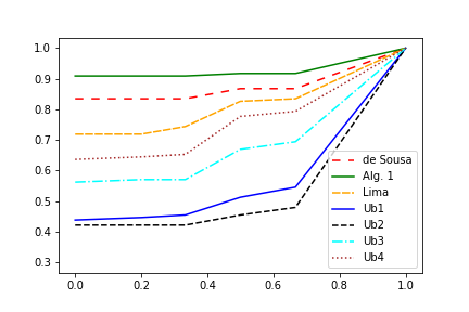
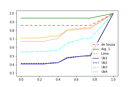
One source	Two sources

Figure 1: Performance profiles of the upper bounding methods

Figure 1 summarise all experiments reported in Tabs. 6.2–6.3 in terms of performance profiles. Two separate sets of profiles are given for the cases $\sigma=1$ and $\sigma=2$ for comparison of all upper bounding methods (Fig. 1), including the two time-constrained ILP approaches.

The dominance of Alg. 1 (profile ‘Alg. 1’) over the model of de Sousa et al. (2018a, b) (profile ‘de Sousa’) is highly visible in Fig. 1. Reflecting the fact that Alg. 1 solves most of the instances to optimality, and provides the best upper bound in most of the remaining instances, the ordinate values of the left-most points of the corresponding performance profiles are larger than 90% and 95% for the single-source and double-source experiments, respectively.

A comparison of the heuristic methods shows that in the single-source instances, the genetic algorithm of Lima et al. (2022) (profile ‘Lima’) performs better than Alg. 3 (profile ‘Ub$\kappa$’) for all $\kappa=1,\ldots,4$. For $\sigma=2$, however, this is true only when $\kappa\leq 3$, and Alg. 3 becomes competitive when $\kappa=4$. The favourable performance of the genetic algorithm is also mainly explained by better results in the smaller instances. Figure 2 depicts the performance profiles confined to the instances in which $|V|\geq 1000$, including both $\sigma=1$ and $\sigma=2$. Among the instances excluded by this criterion, Alg. 1 solves to optimality all but two single-source instances, which justifies the focus to the restricted instance set.

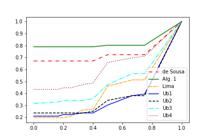
Figure 2: Performance profiles of the upper bounding methods in instances where $|V|\geq 1000$

It is observed from Fig. 2 that Alg. 3 performs better than the genetic algorithm (Lima et al., 2022), provided that $\kappa\geq 3$. For $\kappa=3$, the difference is modest, whereas it becomes significant for $\kappa=4$. Figures 1–2 also show that there is no added value of increasing the value of $\kappa$ from 1 to 2 in Alg. 3.

6.4 Solution time

Tables C.1–C.2 report solution times in seconds for all but one of the methods analysed in Section 6.3 in all instances of some computational challenge. Since in the majority of the instances, the method of Lima et al. (2022) continues the search as long as the given time limit (60s for each of 21 seed values) is not reached, it is excluded from the solution time analysis. In an order consistent with Tabs. B.1–B.8, columns 2–7 (columns 8–13) contain the running times for single-source (double-source) instances. Arguing that running time is unlikely to be an issue in instances for which optimality is provable in a one-digit number of seconds, we include only instances in which at least one method needs 10 seconds or more to conclude. A stroke (‘–’) is given for trivial instances (see Section 6.2), and, in line with Tabs. B.1–B.8, the symbol ‘†’ corresponds to runs interrupted by memory shortage. For each instance set, average running times are given in Tab. 6.4, where runs exhausting the memory are considered to take 3600 seconds.

Table 6.4: Running times (seconds) averaged over all instances ($|S|\in\{1,2\}$) in each set

	ILP approaches			Heuristics
Instance set	de Sousa	Alg1		Ub1	Ub2	Ub3	Ub4
Geometric	831.7	162.0		1.0	1.6	2.3	3.2
Harary	0.4	0.1		0.0	0.0	0.0	0.0
Hypercube	675.5	696.4		0.1	0.2	0.5	4.4
CC cycles	4.2	7.7		0.1	0.1	0.2	0.2
de Bruijn	792.3	102.0		0.1	0.1	0.2	0.3
Shuffle exchange	42.1	17.4		0.1	0.2	0.3	0.4
Synthetic ($|V|=32$)	0.2	0.1		0.0	0.0	0.0	0.0
Synthetic ($|V|=64$)	1.1	0.2		0.0	0.0	0.1	0.1
Synthetic ($|V|=128$)	49.7	1.9		0.1	0.1	0.3	0.5
Synthetic ($|V|=256$)	1187.7	36.3		0.2	0.6	1.6	3.6
Synthetic ($|V|=512$)	3607.2	573.5		0.6	3.2	11.2	29.2
Synthetic ($|V|=1024$)	3600.0	3611.2		2.4	18.0	81.2	287.5
Small world ($|V|=10^{2}$, $|E|=2|V|$)	2.6	0.4		0.0	0.0	0.1	0.1
Small world ($|V|=10^{2}$, $|E|=3|V|$)	2.7	0.5		0.0	0.0	0.1	0.2
Small world ($|V|=10^{3}$, $|E|=2|V|$)	2304.7	595.9		0.2	0.4	0.8	3.3
Small world ($|V|=10^{3}$, $|E|=3|V|$)	2596.5	761.0		0.3	0.4	0.9	13.6

Computational superiority of Alg. 1 over model (1) is confirmed by the running times. The latter approach is, however, faster in 10 instances. The most significant difference in its favour is found in the double-source instance of graph rgg-1000-2792, in which Alg. 1 needed almost seven times the running time of (1). Other instances that are exceptions to the general rule, are the graphs cubeconnectedcycles7 ($\sigma=1,2$), shuffle_exchange10 ($\sigma=1$), rgg-1200-3855 ($\sigma=2$), hypercube8 ($\sigma=2$), hypercube9 ($\sigma=2$), SW-1000-4-0d3-trial2 ($\sigma=1$), SW-1000-6-0d2-trial3 ($\sigma=1$), SW-1000-5-0d1-trial3 ($\sigma=2$), and SW-1000-6-0d2-trial3 ($\sigma=2$). But in 52 of the instances that both could solve to optimality, Alg. 1 spent less than half the time the solver needed to solve the model of de Sousa et al. (2018a, b). A graphic illustration is given in Fig. 3, which shows the running time of Alg. 1 versus the model of de Sousa et al. (2018a, b) in all said instances.

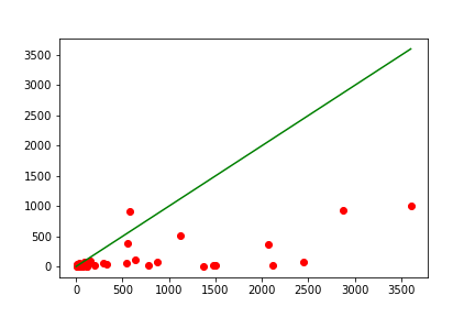
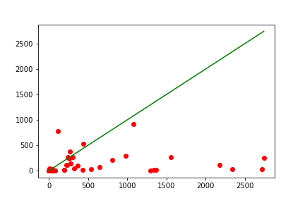
One source	Two sources

Figure 3: Running times (seconds) of Alg. 1 (vertical axis) vs running times of model (1) (horizontal axis)

As expected, the running time of heuristic Alg. 3 increases with increasing value of the parameter $\kappa$. In all small world instances but one, however, and in all other instances except five (six) of the more challenging single-source (double-source) instances of synthetic graphs, the running time is kept below two minutes, even for $\kappa=4$.

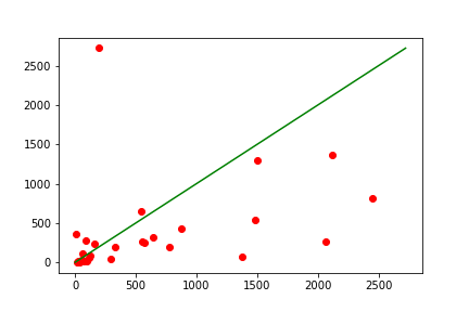
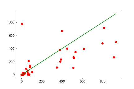
Model (1)(de Sousa et al., 2018a, b)	Alg. 1

Figure 4: Running times (seconds) of the ILP approaches applied to double-source instances (vertical axis) vs single-source instances (horizontal axis)

When comparing the single-source and the double-source instances corresponding to the same graph, the experiments give no conclusive evidence that either source cardinality is more or less challenging. For both ILP approaches under consideration, Fig. 4 plots the running times of the double-source instances against the running time of its single-source counterpart. This is done for all graphs where the ILP approach was able to solve both instances to optimality within the time limit. Visual inspection suggests a bias towards the conclusion that the single-source instances are somewhat more challenging. Algorithm 1 fails to prove optimality in 16 single-source and 15 double-source instances. Out of 40 graphs for which both instances are non-trivial, and the algorithm solves both to optimality, and needs at least 10 seconds to do so, the single-source (double-source) instance is solved faster for 12 (28) graphs.

7 Concluding Remarks

This work focuses on the minimum broadcast time problem, and presents several techniques for computing lower bounds, upper bounds, as well as optimal solutions. Particular attention is given to a procedure which in each iteration solves an integer linear programming model. When run exhaustively, this procedure solves the problem. Otherwise, it computes a lower bound on the broadcast time. The same procedure applied to the continuous relaxation of the model is also capable of computing a lower bound. Further, an upper-bounding iterative technique is studied. This method solves a sequence of subproblems, each of which is a possibly small instance of the integer program. With its parameter decisive for the size of the subproblem instances, the upper bounding method offers high flexibility in the trade-off between sharpness of the bound and computational effort.

For experimental evaluation of the computational procedures, various instance classes of variable size are addressed. While most instance sets are identical to those studied in a recently published work on the same problem, also new, randomly generated instances are studied. The random instances are intended to simulate real communication networks.

Computational experiments demonstrate that the majority of the instances that cannot be solved by fast bound-computing algorithms, are solved by the procedure generating a sequence of integer linear programs. When interrupted because the time limit is reached, the procedure produces bounds that are generally stronger than those produced within the same time limit by a previously studied ILP model. In such instances, where the exact approach fails to prove optimality, the heuristic developed in the current work outputs solutions superior to those produced by a recently studied metaheuristic, and does so with modest computational effort.

There is a potential for future research in developing stronger upper bounding algorithms and improving the existing ILP model. Although the model formulation is compact, its size represents a challenge due to a cubic number of variables. Model improvements can be achieved by not only introduction of redundant valid inequalities, but also by developing conceptually different models, where the number of variables is reduced by an order of magnitude.

SUPPLEMENTARY MATERIAL

Appendix A Lower and upper bounds

Table A.1: Lower and upper bounds - geometric graphs on the unit sphere

	Size			$|S|=1$				$|S|=2$
Instance	$|V|$	$|E|$		degree	$\max$ sp	ub		degree	$\max$ sp	ub
rgg-400-1220	400	1220		9	19	21		8	18	19
rgg-400-1264	400	1264		9	23	23∗		8	23	23∗
rgg-400-1779	400	1779		9	13	17		8	11	14
rgg-400-1816	400	1816		9	14	16		8	12	14
rgg-600-1027	600	1027		10	208	208∗		9	140	140∗
rgg-600-1087	600	1087		10	255	255∗		9	110	110∗
rgg-600-1833	600	1833		10	32	32∗		9	23	24
rgg-600-1861	600	1861		10	40	40∗		9	24	24∗
rgg-800-1034	800	1034		11	568	568∗		10	295	296
rgg-800-1067	800	1067		11	540	540∗		9	365	365∗
rgg-800-1868	800	1868		10	118	118∗		9	48	48∗
rgg-800-1871	800	1871		10	97	97∗		9	86	86∗
rgg-1000-1447	1000	1447		11	598	598∗		10	525	525∗
rgg-1000-1460	1000	1460		11	591	591∗		10	492	494
rgg-1000-2792	1000	2792		10	43	44		9	31	32
rgg-1000-2827	1000	2827		11	51	51∗		10	30	32
rgg-1200-1940	1200	1940		11	603	603∗		10	368	368∗
rgg-1200-1965	1200	1965		11	573	573∗		10	495	495∗
rgg-1200-3855	1200	3855		11	36	36∗		10	28	29
rgg-1200-4075	1200	4075		11	36	36∗		10	24	24∗

Table A.2: Lower and upper bounds - miscellaneous graphs

	Size			$|S|=1$				$|S|=2$
Instance	$|V|$	$|E|$		degree	$\max$ sp	ub		degree	$\max$ sp	ub
harary17c2	17	17		9	8	9∗		5	7	7∗
harary17c3	17	26		5	5	6		4	4	5
harary17c5	17	43		5	3	6		4	2	4∗
harary17c6	17	51		5	3	5∗		4	2	4∗
harary17c7	17	60		5	2	5∗		4	2	4∗
harary30c2	30	30		15	15	15∗		8	11	11∗
harary30c3	30	45		6	8	9		5	8	8∗
harary30c8	30	120		5	4	6		4	3	5
harary30c9	30	135		5	3	6		4	2	5
harary30c10	30	150		5	3	6		4	3	5
harary50c2	50	50		25	25	25∗		13	25	25∗
harary50c3	50	75		7	13	14		6	12	12∗
harary50c11	50	275		6	3	7		5	3	6
harary50c20	50	500		6	3	7		5	3	6
harary50c21	50	525		6	2	8		5	2	5∗
harary100c2	100	100		50	50	50∗		25	28	28∗
hypercube5	32	80		5	5	5∗		4	4	5
hypercube6	64	192		6	6	6∗		5	4	6
hypercube7	128	448		7	7	7∗		6	4	7
hypercube8	256	1024		8	8	8∗		7	6	8
hypercube9	512	2304		9	9	9∗		8	8	9
hypercube10	1024	5120		10	10	10∗		9	9	10
cubeconnectedcycles3	24	36		5	6	7		4	4	5
cubeconnectedcycles4	64	96		7	8	9		6	6	7
cubeconnectedcycles5	160	240		9	10	12		8	9	10
cubeconnectedcycles6	384	576		11	13	14		10	11	13
cubeconnectedcycles7	896	1344		13	15	17		11	14	15
debruijn04	16	31		4	4	5		3	3	5
debruijn05	32	63		6	5	7		4	4	7
debruijn06	64	127		7	6	8		6	6	7
debruijn07	128	255		8	7	10		7	6	9
debruijn08	256	511		9	8	12		8	7	10
debruijn09	512	1023		10	9	14		9	8	13
debruijn10	1024	2047		11	10	16		10	9	15
shuffle_exchange4	16	21		6	7	7∗		4	3	4∗
shuffle_exchange5	32	46		7	9	9∗		5	8	8∗
shuffle_exchange6	64	93		9	11	11∗		7	7	8
shuffle_exchange7	128	190		10	13	14		8	9	11
shuffle_exchange8	256	381		12	15	16		9	13	14
shuffle_exchange9	512	766		13	17	18		11	12	14
shuffle_exchange10	1024	1533		15	19	20		12	13	17

Table A.3: Lower and upper bounds - synthetic graphs

	Size			$|S|=1$				$|S|=2$
Instance	$|V|$	$|E|$		degree	$\max$ sp	ub		degree	$\max$ sp	ub
BT4	16	15		4	4	4∗		4	4	4∗
BT5	32	31		5	5	5∗		5	4	5∗
BT6	64	63		6	6	6∗		6	6	6∗
BT7	128	127		7	7	7∗		6	6	6∗
BT8	256	255		8	8	8∗		8	8	8∗
BT9	512	511		9	9	9∗		9	9	9∗
BT05_RG050	32	48		5	5	6		4	3	5
BT05_RG075	32	64		5	4	6		4	3	5
BT05_RG100	32	83		5	3	6		4	3	5
BT05_RG150	32	89		5	3	7		4	3	6
BT05_RG200	32	142		5	2	7		4	2	5
BT05_RG250	32	156		5	2	8		4	2	5
BT06_RG050	64	159		6	3	9		6	3	8
BT06_RG075	64	184		6	3	10		6	3	10
BT06_RG100	64	243		6	3	8		5	3	7
BT06_RG150	64	349		6	2	8		5	2	6
BT06_RG200	64	461		6	2	8		5	2	6
BT06_RG250	64	558		6	2	8		5	2	7
BT07_RG050	128	560		7	3	9		7	3	9
BT07_RG075	128	716		7	3	12		6	3	9
BT07_RG100	128	923		7	3	11		6	2	9
BT07_RG150	128	1313		7	3	10		6	2	8
BT07_RG200	128	1742		7	2	10		6	2	8
BT07_RG250	128	2140		7	2	10		6	2	8
BT08_RG050	256	1863		8	3	13		7	3	10
BT08_RG075	256	2657		8	3	12		7	3	11
BT08_RG100	256	3450		8	2	11		7	2	10
BT08_RG150	256	5168		8	2	11		7	2	9
BT08_RG200	256	6691		8	2	11		7	2	10
BT08_RG250	256	8307		8	2	12		7	2	10
BT09_RG050	512	6881		9	3	17		8	3	13
BT09_RG075	512	10304		9	3	13		8	2	11
BT09_RG100	512	13444		9	2	12		8	2	11
BT09_RG150	512	20009		9	2	13		8	2	11
BT09_RG200	512	27012		9	2	13		8	2	12
BT09_RG250	512	33313		9	2	13		8	2	12
BT10_RG050	1024	27259		10	3	16		9	3	13
BT10_RG075	1024	40222		10	3	14		9	2	13
BT10_RG100	1024	53480		10	2	14		9	2	12
BT10_RG150	1024	79574		10	2	14		9	2	13
BT10_RG200	1024	105448		10	2	15		9	2	13
BT10_RG250	1024	131643		10	2	15		9	2	12

Table A.4: Lower and upper bounds - small world ($|V|=100$) graphs

	Size			$|S|=1$				$|S|=2$
Instance	$|V|$	$|E|$		degree	$\max$ sp	ub		degree	$\max$ sp	ub
SW-100-3-0d1-trial1	100	100		11	61	61∗		9	22	22∗
SW-100-3-0d2-trial1	100	100		12	31	31∗		10	31	31∗
SW-100-3-0d2-trial3	100	100		12	31	31∗		10	31	31∗
SW-100-4-0d1-trial1	100	200		7	7	11		6	7	9
SW-100-4-0d1-trial2	100	200		7	7	10		6	5	8
SW-100-4-0d1-trial3	100	200		7	9	11		6	7	9
SW-100-4-0d2-trial1	100	200		7	7	9		6	6	8
SW-100-4-0d2-trial2	100	200		7	7	10		6	6	9
SW-100-4-0d2-trial3	100	200		7	7	10		6	6	9
SW-100-4-0d3-trial1	100	200		7	6	9		6	6	9
SW-100-4-0d3-trial2	100	200		7	6	9		6	6	9
SW-100-4-0d3-trial3	100	200		7	7	9		6	6	8
SW-100-5-0d1-trial1	100	200		7	8	11		6	7	9
SW-100-5-0d1-trial2	100	200		7	9	10		6	7	9
SW-100-5-0d1-trial3	100	200		7	11	14		6	8	9
SW-100-5-0d2-trial1	100	200		7	8	11		6	5	8
SW-100-5-0d2-trial2	100	200		7	9	10		6	6	9
SW-100-5-0d2-trial3	100	200		7	7	9		6	6	8
SW-100-5-0d3-trial1	100	200		7	6	9		6	5	8
SW-100-5-0d3-trial2	100	200		7	6	9		6	6	8
SW-100-5-0d3-trial3	100	200		7	6	10		6	6	8
SW-100-6-0d1-trial1	100	300		7	5	9		6	4	8
SW-100-6-0d1-trial2	100	300		7	6	9		6	4	8
SW-100-6-0d1-trial3	100	300		7	6	9		6	6	7
SW-100-6-0d2-trial1	100	300		7	6	9		6	4	8
SW-100-6-0d2-trial2	100	300		7	4	8		6	4	8
SW-100-6-0d2-trial3	100	300		7	4	10		6	4	8
SW-100-6-0d3-trial1	100	300		7	4	9		6	4	7
SW-100-6-0d3-trial2	100	300		7	5	9		6	4	8
SW-100-6-0d3-trial3	100	300		7	5	8		6	4	7

Table A.5: Lower and upper bounds - small world ($|V|=1000$) graphs

	Size			$|S|=1$				$|S|=2$
Instance	$|V|$	$|E|$		degree	$\max$ sp	ub		degree	$\max$ sp	ub
SW-1000-3-0d2-trial1	1000	1000		14	89	89∗		13	89	89∗
SW-1000-3-0d2-trial2	1000	1000		14	88	88∗		13	81	81∗
SW-1000-3-0d3-trial2	1000	1000		13	87	87∗		12	52	52∗
SW-1000-4-0d1-trial1	1000	2000		11	14	18		10	12	15
SW-1000-4-0d1-trial2	1000	2000		11	15	18		10	14	16
SW-1000-4-0d1-trial3	1000	2000		11	15	18		10	13	16
SW-1000-4-0d2-trial1	1000	2000		11	10	16		10	10	14
SW-1000-4-0d2-trial2	1000	2000		11	10	15		10	9	14
SW-1000-4-0d2-trial3	1000	2000		11	11	16		10	10	14
SW-1000-4-0d3-trial1	1000	2000		11	9	14		10	9	13
SW-1000-4-0d3-trial2	1000	2000		11	11	14		10	9	13
SW-1000-4-0d3-trial3	1000	2000		11	8	14		10	8	13
SW-1000-5-0d1-trial1	1000	2000		11	14	17		10	14	17
SW-1000-5-0d1-trial2	1000	2000		11	15	17		10	12	15
SW-1000-5-0d1-trial3	1000	2000		11	12	16		10	12	15
SW-1000-5-0d2-trial1	1000	2000		11	11	15		10	11	14
SW-1000-5-0d2-trial2	1000	2000		11	10	15		10	9	13
SW-1000-5-0d2-trial3	1000	2000		11	10	15		10	9	13
SW-1000-5-0d3-trial1	1000	2000		11	9	14		10	9	13
SW-1000-5-0d3-trial2	1000	2000		11	9	14		10	8	13
SW-1000-5-0d3-trial3	1000	2000		11	10	15		10	8	14
SW-1000-6-0d1-trial1	1000	3000		10	10	15		9	9	15
SW-1000-6-0d1-trial2	1000	3000		10	10	15		10	9	13
SW-1000-6-0d1-trial3	1000	3000		11	8	15		9	8	13
SW-1000-6-0d2-trial1	1000	3000		10	8	14		9	7	13
SW-1000-6-0d2-trial2	1000	3000		11	8	14		10	7	13
SW-1000-6-0d2-trial3	1000	3000		11	7	14		10	7	12
SW-1000-6-0d3-trial1	1000	3000		10	6	13		9	6	13
SW-1000-6-0d3-trial2	1000	3000		10	6	14		10	6	13
SW-1000-6-0d3-trial3	1000	3000		11	7	13		10	7	12

Appendix B ILP approaches and heuristics

Table B.1: Results from experiments with ILP approaches and heuristics - miscellaneous single-source instances

	ILP approaches						Heuristics
	de Sousa			Alg1					Alg3
Instance	lb	ub		lb	ub		Lima		Ub1	Ub2	Ub3	Ub4
rgg-400-1220	20	20∗		20	20∗		20∗		22	22	22	22
rgg-400-1779	15	15∗		15	15∗		15∗		17	17	16	16
rgg-400-1816	15	15∗		15	15∗		16		17	17	17	17
rgg-1000-2792	44	44∗		44	44∗		44∗		45	49	45	45
harary17c3	6	6∗		6	6∗		6∗		6∗	6∗	6∗	6∗
harary17c5	5	5∗		5	5∗		5∗		5∗	5∗	5∗	5∗
harary30c3	9	9∗		9	9∗		9∗		9∗	9∗	9∗	9∗
harary30c8	5	5∗		5	5∗		5∗		6	6	6	6
harary30c9	5	5∗		5	5∗		5∗		5∗	5∗	5∗	5∗
harary30c10	5	5∗		5	5∗		5∗		5∗	6	5∗	5∗
harary50c3	14	14∗		14	14∗		14∗		14∗	14∗	14∗	14∗
harary50c11	6	6∗		6	6∗		6∗		6∗	6∗	6∗	6∗
harary50c20	6	6∗		6	6∗		6∗		6∗	6∗	6∗	6∗
harary50c21	6	6∗		6	6∗		6∗		6∗	6∗	6∗	6∗
cubeconnectedcycles3	6	6∗		6	6∗		6∗		7	7	6∗	7
cubeconnectedcycles4	9	9∗		9	9∗		9∗		10	9∗	9∗	9∗
cubeconnectedcycles5	11	11∗		11	11∗		11∗		13	13	12	12
cubeconnectedcycles6	13	13∗		13	13∗		13∗		15	15	15	15
cubeconnectedcycles7	16	16∗		16	16∗		16∗		17	18	17	18
debruijn04	5	5∗		5	5∗		5∗		5∗	5∗	5∗	5∗
debruijn05	6	6∗		6	6∗		6∗		7	7	6∗	6∗
debruijn06	8	8∗		8	8∗		8∗		8∗	8∗	8∗	8∗
debruijn07	9	9∗		9	9∗		9∗		10	10	9∗	9∗
debruijn08	10	10∗		10	10∗		11		12	12	11	11
debruijn09	12	12∗		12	12∗		13		13	13	12∗	12∗
debruijn10	13	14		13	13∗		14		15	15	15	14
shuffle_exchange7	13	13∗		13	13∗		13∗		14	14	14	14
shuffle_exchange8	15	15∗		15	15∗		15∗		16	17	18	17
shuffle_exchange9	17	17∗		17	17∗		17∗		19	19	19	19
shuffle_exchange10	19	19∗		19	19∗		20		21	21	21	22

Table B.2: Results from experiments with ILP approaches and heuristics - synthetic single-source instances

	ILP approaches						Heuristics
	de Sousa			Alg1					Alg3
Instance	lb	ub		lb	ub		Lima		Ub1	Ub2	Ub3	Ub4
BT05_RG050	5	5∗		5	5∗		5∗		6	6	5∗	5∗
BT05_RG075	5	5∗		5	5∗		5∗		6	6	5∗	5∗
BT05_RG100	5	5∗		5	5∗		5∗		6	5∗	5∗	5∗
BT05_RG150	5	5∗		5	5∗		5∗		5∗	5∗	5∗	5∗
BT05_RG200	5	5∗		5	5∗		5∗		5∗	5∗	5∗	5∗
BT05_RG250	5	5∗		5	5∗		5∗		5∗	5∗	5∗	5∗
BT06_RG050	6	6∗		6	6∗		6∗		7	7	7	6∗
BT06_RG075	6	6∗		6	6∗		6∗		7	6∗	6∗	6∗
BT06_RG100	6	6∗		6	6∗		6∗		6∗	6∗	7	6∗
BT06_RG150	6	6∗		6	6∗		6∗		6∗	6∗	6∗	6∗
BT06_RG200	6	6∗		6	6∗		6∗		6∗	6∗	6∗	6∗
BT06_RG250	6	6∗		6	6∗		6∗		6∗	6∗	6∗	6∗
BT07_RG050	7	7∗		7	7∗		7∗		7∗	8	7∗	7∗
BT07_RG075	7	7∗		7	7∗		7∗		7∗	7∗	7∗	7∗
BT07_RG100	7	7∗		7	7∗		7∗		7∗	7∗	7∗	7∗
BT07_RG150	7	7∗		7	7∗		7∗		7∗	7∗	7∗	7∗
BT07_RG200	7	7∗		7	7∗		7∗		7∗	7∗	7∗	7∗
BT07_RG250	7	7∗		7	7∗		7∗		7∗	7∗	7∗	7∗
BT08_RG050	8	8∗		8	8∗		8∗		8∗	8∗	8∗	8∗
BT08_RG075	8	8∗		8	8∗		8∗		8∗	8∗	8∗	8∗
BT08_RG100	8	8∗		8	8∗		8∗		8∗	8∗	8∗	8∗
BT08_RG150	8	8∗		8	8∗		8∗		8∗	8∗	8∗	8∗
BT08_RG200	8	8∗		8	8∗		8∗		8∗	8∗	8∗	8∗
BT08_RG250	†	†		8	8∗		8∗		8∗	8∗	8∗	8∗
BT09_RG050	9	–		9	10		10		9∗	9∗	9∗	9∗
BT09_RG075	†	†		9	10		10		9∗	9∗	9∗	9∗
BT09_RG100	†	†		9	9∗		9∗		9∗	9∗	9∗	9∗
BT09_RG150	†	†		9	9∗		9∗		9∗	9∗	9∗	9∗
BT09_RG200	†	†		9	9∗		9∗		9∗	9∗	9∗	9∗
BT09_RG250	†	†		9	9∗		9∗		9∗	9∗	9∗	9∗
BT10_RG050	†	†		10	–		11		10∗	10∗	10∗	10∗
BT10_RG075	†	†		10	–		11		10∗	10∗	10∗	10∗
BT10_RG100	†	†		10	–		10∗		10∗	10∗	10∗	10∗
BT10_RG150	†	†		10	–		10∗		10∗	10∗	10∗	10∗
BT10_RG200	†	†		10	–		10∗		10∗	10∗	10∗	10∗
BT10_RG250	†	†		10	–		10∗		10∗	10∗	10∗	10∗

Table B.3: Results from experiments with ILP approaches and heuristics - small world ($|V|=100$) single-source instances

	ILP approaches						Heuristics
	de Sousa			Alg1					Alg3
Instance	lb	ub		lb	ub		Lima		Ub1	Ub2	Ub3	Ub4
SW-100-4-0d1-trial1	9	9∗		9	9∗		9∗		10	10	10	9∗
SW-100-4-0d1-trial2	8	8∗		8	8∗		8∗		9	9	9	9
SW-100-4-0d1-trial3	10	10∗		10	10∗		10∗		11	11	11	10∗
SW-100-4-0d2-trial1	8	8∗		8	8∗		8∗		9	10	9	8∗
SW-100-4-0d2-trial2	8	8∗		8	8∗		8∗		9	9	9	9
SW-100-4-0d2-trial3	9	9∗		9	9∗		9∗		9∗	10	9∗	9∗
SW-100-4-0d3-trial1	8	8∗		8	8∗		8∗		9	10	9	9
SW-100-4-0d3-trial2	8	8∗		8	8∗		8∗		8∗	8∗	8∗	8∗
SW-100-4-0d3-trial3	8	8∗		8	8∗		8∗		9	9	9	8∗
SW-100-5-0d1-trial1	9	9∗		9	9∗		9∗		10	10	10	10
SW-100-5-0d1-trial2	10	10∗		10	10∗		10∗		11	11	11	11
SW-100-5-0d1-trial3	12	12∗		12	12∗		12∗		13	13	12∗	12∗
SW-100-5-0d2-trial1	9	9∗		9	9∗		9∗		11	11	10	10
SW-100-5-0d2-trial2	9	9∗		9	9∗		9∗		11	11	10	10
SW-100-5-0d2-trial3	8	8∗		8	8∗		8∗		9	9	10	9
SW-100-5-0d3-trial1	8	8∗		8	8∗		8∗		9	9	8∗	8∗
SW-100-5-0d3-trial2	8	8∗		8	8∗		8∗		8∗	8∗	8∗	8∗
SW-100-5-0d3-trial3	8	8∗		8	8∗		8∗		8∗	9	8∗	8∗
SW-100-6-0d1-trial1	7	7∗		7	7∗		7∗		8	8	8	8
SW-100-6-0d1-trial2	8	8∗		8	8∗		8∗		8∗	9	8∗	8∗
SW-100-6-0d1-trial3	7	7∗		7	7∗		7∗		9	8	8	8
SW-100-6-0d2-trial1	7	7∗		7	7∗		7∗		8	8	8	7∗
SW-100-6-0d2-trial2	7	7∗		7	7∗		7∗		7∗	7∗	7∗	7∗
SW-100-6-0d2-trial3	7	7∗		7	7∗		7∗		8	8	7∗	7∗
SW-100-6-0d3-trial1	7	7∗		7	7∗		7∗		7∗	8	7∗	7∗
SW-100-6-0d3-trial2	7	7∗		7	7∗		7∗		7∗	8	7∗	7∗
SW-100-6-0d3-trial3	7	7∗		7	7∗		7∗		7∗	7∗	7∗	7∗

Table B.4: Results from experiments with ILP approaches and heuristics - small world ($|V|=1000$) single-source instances

	ILP approaches						Heuristics
	de Sousa			Alg1					Alg3
Instance	lb	ub		lb	ub		Lima		Ub1	Ub2	Ub3	Ub4
SW-1000-4-0d1-trial1	15	15∗		15	15∗		16		17	18	17	18
SW-1000-4-0d1-trial2	16	16∗		16	16∗		17		18	18	19	17
SW-1000-4-0d1-trial3	16	16∗		16	16∗		17		18	18	18	18
SW-1000-4-0d2-trial1	12	13		12	13		14		14	14	15	14
SW-1000-4-0d2-trial2	12	13		12	13		14		14	15	14	14
SW-1000-4-0d2-trial3	13	13∗		13	13∗		15		15	16	15	15
SW-1000-4-0d3-trial1	11	12		11	12		13		13	13	13	13
SW-1000-4-0d3-trial2	12	12∗		12	12∗		14		14	14	14	14
SW-1000-4-0d3-trial3	11	12		11	12		13		14	13	13	12
SW-1000-5-0d1-trial1	16	16∗		16	16∗		16∗		18	18	18	18
SW-1000-5-0d1-trial2	16	16∗		16	16∗		16∗		18	18	18	17
SW-1000-5-0d1-trial3	14	14∗		14	14∗		15		16	16	16	16
SW-1000-5-0d2-trial1	13	13∗		13	13∗		14		15	15	15	14
SW-1000-5-0d2-trial2	12	13		12	12∗		14		14	14	14	14
SW-1000-5-0d2-trial3	12	13		12	12∗		14		14	14	14	13
SW-1000-5-0d3-trial1	11	12∗		12	12∗		13		13	13	13	13
SW-1000-5-0d3-trial2	11	12		11	12		13		13	13	13	13
SW-1000-5-0d3-trial3	11	12∗		12	12∗		13		14	14	14	13
SW-1000-6-0d1-trial1	12	14		12	12∗		14		14	14	14	14
SW-1000-6-0d1-trial2	12	14		12	12∗		14		14	14	14	14
SW-1000-6-0d1-trial3	11	12		11	13		13		13	13	13	12
SW-1000-6-0d2-trial1	10	12		11	12		12		12	12	11∗	11∗
SW-1000-6-0d2-trial2	11	12		11	12		13		12	13	12	11∗
SW-1000-6-0d2-trial3	11	11∗		11	11∗		12		12	12	11∗	11∗
SW-1000-6-0d3-trial1	10	11∗		11	11∗		12		11∗	11∗	11∗	11∗
SW-1000-6-0d3-trial2	10	11∗		11	11∗		12		11∗	11∗	11∗	11∗
SW-1000-6-0d3-trial3	11	11∗		11	11∗		12		12	11∗	11∗	11∗

Table B.5: Results from experiments with ILP approaches and heuristics - miscellaneous double-source instances

	ILP approaches						Heuristics
	de Sousa			Alg1					Alg3
Instance	lb	ub		lb	ub		Lima		Ub1	Ub2	Ub3	Ub4
rgg-400-1220	18	18∗		18	18∗		18∗		19	21	19	19
rgg-400-1779	12	12∗		12	12∗		12∗		15	14	14	13
rgg-400-1816	13	13∗		13	13∗		14		16	16	15	16
rgg-600-1833	23	23∗		23	23∗		23∗		24	25	23∗	24
rgg-800-1034	296	296∗		296	296∗		296∗		298	299	298	296∗
rgg-1000-1460	†	†		494	494∗		494∗		496	500	495	494∗
rgg-1000-2792	31	31∗		31	31∗		31∗		36	33	33	33
rgg-1000-2827	31	31∗		31	31∗		31∗		34	34	33	32
rgg-1200-3855	28	28∗		28	28∗		29		31	32	30	31
harary17c3	5	5∗		5	5∗		5∗		5∗	5∗	5∗	5∗
harary30c8	4	4∗		4	4∗		4∗		5	5	4∗	4∗
harary30c9	4	4∗		4	4∗		4∗		4∗	4∗	4∗	4∗
harary30c10	4	4∗		4	4∗		4∗		4∗	4∗	4∗	4∗
harary50c11	5	5∗		5	5∗		5∗		5∗	5∗	5∗	5∗
harary50c20	5	5∗		5	5∗		5∗		5∗	5∗	5∗	5∗
hypercube5	4	4∗		4	4∗		4∗		4∗	4∗	4∗	4∗
hypercube6	5	5∗		5	5∗		5∗		6	6	6	5∗
hypercube7	6	6∗		6	6∗		6∗		7	7	6∗	6∗
hypercube8	7	7∗		7	7∗		7∗		8	8	8	7∗
hypercube9	8	8∗		8	8∗		9		9	9	9	8∗
hypercube10	9	–		9	–		10		10	10	10	10
cubeconnectedcycles3	5	5∗		5	5∗		5∗		5∗	5∗	5∗	5∗
cubeconnectedcycles4	6	6∗		6	6∗		6∗		7	7	7	7
cubeconnectedcycles5	10	10∗		10	10∗		10∗		10∗	11	10∗	10∗
cubeconnectedcycles6	12	12∗		12	12∗		12∗		14	14	13	13
cubeconnectedcycles7	15	15∗		15	15∗		15∗		16	16	16	16
debruijn04	4	4∗		4	4∗		4∗		4∗	4∗	4∗	4∗
debruijn05	5	5∗		5	5∗		5∗		6	6	6	5∗
debruijn06	6	6∗		6	6∗		6∗		7	7	7	7
debruijn07	7	7∗		7	7∗		7∗		8	8	8	8
debruijn08	9	9∗		9	9∗		9∗		10	10	10	9∗
debruijn09	10	10∗		10	10∗		11		12	12	12	11
debruijn10	11	12		11	12		13		14	13	13	12
shuffle_exchange6	8	8∗		8	8∗		8∗		9	8∗	8∗	8∗
shuffle_exchange7	10	10∗		10	10∗		10∗		11	12	10∗	11
shuffle_exchange8	13	13∗		13	13∗		13∗		14	14	14	15
shuffle_exchange9	13	13∗		13	13∗		13∗		14	14	15	15
shuffle_exchange10	14	14∗		14	14∗		15		17	17	16	17

Table B.6: Results from experiments with ILP approaches and heuristics - synthetic double-source instances

ILP approaches

Heuristics

de Sousa

Alg1

Alg3

Instance

lb

ub

lb

ub

Lima

Ub1

Ub2

Ub3

Ub4

BT05_RG050

4

4∗

4

4∗

4∗

5

5

5

4∗

BT05_RG075

4

4∗

4

4∗

4∗

5

5

4∗

4∗

BT05_RG100

4

4∗

4

4∗

4∗

5

4∗

4∗

4∗

BT05_RG150

4

4∗

4

4∗

4∗

5

4∗

4∗

4∗

BT05_RG200

4

4∗

4

4∗

4∗

4∗

4∗

4∗

4∗

BT05_RG250

4

4∗

4

4∗

4∗

4∗

4∗

4∗

4∗

BT06_RG050

6

6∗

6

6∗

6∗

6∗

6∗

6∗

6∗

BT06_RG075

6

6∗

6

6∗

6∗

6∗

6∗

6∗

6∗

BT06_RG100

5

5∗

5

5∗

5∗

5∗

6

6

5∗

BT06_RG150

5

5∗

5

5∗

5∗

5∗

5∗

5∗

5∗

BT06_RG200

5

5∗

5

5∗

5∗

5∗

5∗

5∗

5∗

BT06_RG250

5

5∗

5

5∗

5∗

5∗

5∗

5∗

5∗

BT07_RG050

7

7∗

7

7∗

7∗

7∗

7∗

7∗

7∗

BT07_RG075

6

6∗

6

6∗

6∗

7

7

6∗

6∗

BT07_RG100

6

6∗

6

6∗

6∗

6∗

6∗

6∗

6∗

BT07_RG150

6

6∗

6

6∗

6∗

6∗

6∗

6∗

6∗

BT07_RG200

6

6∗

6

6∗

6∗

6∗

6∗

6∗

6∗

BT07_RG250

6

6∗

6

6∗

6∗

6∗

6∗

6∗

6∗

BT08_RG050

7

7∗

7

7∗

7∗

7∗

7∗

7∗

7∗

BT08_RG075

7

7∗

7

7∗

7∗

7∗

7∗

7∗

7∗

BT08_RG100

7

7∗

7

7∗

7∗

7∗

7∗

7∗

7∗

BT08_RG150

7

7∗

7

7∗

7∗

7∗

7∗

7∗

7∗

BT08_RG200

7

7∗

7

7∗

7∗

7∗

7∗

7∗

7∗

BT08_RG250

7

7∗

7

7∗

7∗

7∗

7∗

7∗

7∗

BT09_RG050

8

–

8

8∗

9

8∗

8∗

8∗

8∗

BT09_RG075

8

–

8

8∗

9

8∗

8∗

8∗

8∗

BT09_RG100

†

†

8

8∗

8∗

8∗

8∗

8∗

8∗

BT09_RG150

†

†

8

8∗

8∗

8∗

8∗

8∗

8∗

BT09_RG200

†

†

8

8∗

8∗

8∗

8∗

8∗

8∗

BT09_RG250

†

†

8

8∗

8∗

8∗

8∗

8∗

8∗

BT10_RG050

†

†

9

–

10

9∗

9∗

9∗

9∗

BT10_RG075

†

†

9

–

10

9∗

9∗

9∗

9∗

BT10_RG100

†

†

10

12

12

10∗

10∗

10∗

10∗

BT10_RG150

†

†

9

–

9∗

9∗

9∗

9∗

9∗

BT10_RG200

†

†

9

–

9∗

9∗

9∗

9∗

9∗

BT10_RG250

†

†

9

–

9∗

9∗

9∗

9∗

9∗

Table B.7: Results from experiments with ILP approaches and heuristics - small world ($|V|=100$) double-source instances

ILP approaches

Heuristics

de Sousa

Alg1

Alg3

Instance

lb

ub

lb

ub

Lima

Ub1

Ub2

Ub3

Ub4

SW-100-4-0d1-trial1

8

8∗

8

8∗

8∗

8∗

8∗

8∗

8∗

SW-100-4-0d1-trial2

7

7∗

7

7∗

7∗

8

7∗

7∗

7∗

SW-100-4-0d1-trial3

8

8∗

8

8∗

8∗

9

10

10

9

SW-100-4-0d2-trial1

7

7∗

7

7∗

7∗

8

8

8

8

SW-100-4-0d2-trial2

8

8∗

8

8∗

8∗

9

8∗

8∗

8∗

SW-100-4-0d2-trial3

7

7∗

7

7∗

7∗

8

8

8

7∗

SW-100-4-0d3-trial1

7

7∗

7

7∗

7∗

9

9

9

8

SW-100-4-0d3-trial2

7

7∗

7

7∗

7∗

7∗

7∗

7∗

7∗

SW-100-4-0d3-trial3

7

7∗

7

7∗

7∗

8

8

8

8

SW-100-5-0d1-trial1

8

8∗

8

8∗

8∗

9

9

8∗

8∗

SW-100-5-0d1-trial2

8

8∗

8

8∗

8∗

8∗

8∗

8∗

8∗

SW-100-5-0d1-trial3

9

9∗

9

9∗

9∗

9∗

10

9∗

9∗

SW-100-5-0d2-trial1

7

7∗

7

7∗

7∗

8

8

8

7∗

SW-100-5-0d2-trial2

7

7∗

7

7∗

7∗

9

9

8

8

SW-100-5-0d2-trial3

7

7∗

7

7∗

7∗

8

8

7∗

7∗

SW-100-5-0d3-trial1

7

7∗

7

7∗

7∗

7∗

7∗

7∗

7∗

SW-100-5-0d3-trial2

6

6∗

6

6∗

6∗

8

7

7

7

SW-100-5-0d3-trial3

7

7∗

7

7∗

7∗

7∗

8

8

7∗

SW-100-6-0d1-trial1

6

6∗

6

6∗

6∗

7

7

7

7

SW-100-6-0d1-trial2

6

6∗

6

6∗

6∗

7

7

7

6∗

SW-100-6-0d1-trial3

6

6∗

6

6∗

6∗

7

7

7

7

SW-100-6-0d2-trial1

6

6∗

6

6∗

6∗

7

7

6∗

6∗

SW-100-6-0d2-trial2

6

6∗

6

6∗

6∗

6∗

6∗

6∗

6∗

SW-100-6-0d2-trial3

6

6∗

6

6∗

6∗

7

7

6∗

6∗

SW-100-6-0d3-trial1

6

6∗

6

6∗

6∗

6∗

6∗

6∗

6∗

SW-100-6-0d3-trial2

6

6∗

6

6∗

6∗

6∗

7

6∗

6∗

SW-100-6-0d3-trial3

6

6∗

6

6∗

6∗

6∗

6∗

6∗

6∗

Table B.8: Results from experiments with ILP approaches and heuristics - small world ($|V|=1000$) double-source instances

	ILP approaches						Heuristics
	de Sousa			Alg1					Alg3
Instance	lb	ub		lb	ub		Lima		Ub1	Ub2	Ub3	Ub4
SW-1000-4-0d1-trial1	13	13∗		13	13∗		15		15	16	16	15
SW-1000-4-0d1-trial2	15	15∗		15	15∗		15∗		16	16	17	16
SW-1000-4-0d1-trial3	14	14∗		14	14∗		15		16	16	16	16
SW-1000-4-0d2-trial1	11	11∗		11	11∗		13		13	13	13	13
SW-1000-4-0d2-trial2	10	11∗		11	11∗		12		12	12	12	11∗
SW-1000-4-0d2-trial3	11	12∗		12	12∗		13		13	13	13	13
SW-1000-4-0d3-trial1	10	11		10	11		12		12	12	12	12
SW-1000-4-0d3-trial2	10	11		10	11		12		13	12	12	11
SW-1000-4-0d3-trial3	10	11		10	11		12		12	12	11	11
SW-1000-5-0d1-trial1	14	14∗		14	14∗		16		16	17	16	17
SW-1000-5-0d1-trial2	13	13∗		13	13∗		15		16	15	15	15
SW-1000-5-0d1-trial3	13	13∗		13	13∗		14		15	15	15	15
SW-1000-5-0d2-trial1	11	12∗		12	12∗		13		13	14	13	13
SW-1000-5-0d2-trial2	11	11∗		11	11∗		13		13	13	13	12
SW-1000-5-0d2-trial3	11	11∗		11	11∗		12		13	12	12	12
SW-1000-5-0d3-trial1	10	11∗		11	11∗		12		12	12	12	12
SW-1000-5-0d3-trial2	10	11		10	11		12		12	12	12	12
SW-1000-5-0d3-trial3	10	11		10	11		12		13	12	12	12
SW-1000-6-0d1-trial1	9	–		11	11∗		13		13	13	13	12
SW-1000-6-0d1-trial2	10	11		10	11		12		12	12	12	12
SW-1000-6-0d1-trial3	10	12		10	11		12		12	12	11	11
SW-1000-6-0d2-trial1	9	11		10	10∗		11		11	11	11	10∗
SW-1000-6-0d2-trial2	10	10∗		10	10∗		11		11	11	11	10∗
SW-1000-6-0d2-trial3	10	10∗		10	10∗		11		11	11	10∗	10∗
SW-1000-6-0d3-trial1	9	11		10	10∗		11		11	10∗	10∗	10∗
SW-1000-6-0d3-trial2	10	10∗		10	10∗		11		10∗	10∗	10∗	10∗
SW-1000-6-0d3-trial3	10	10∗		10	10∗		11		11	11	10∗	10∗

Appendix C Running time

Table C.1: Running times (seconds) - miscellaneous graphs

	$|S|=1$							$|S|=2$
	de		Alg3					de		Alg3
Instance	Sousa	Alg1	Ub1	Ub2	Ub3	Ub4		Sousa	Alg1	Ub1	Ub2	Ub3	Ub4
rgg-400-1220	93	76	0	0	1	1		10	3	0	0	1	1
rgg-400-1779	1505	18	0	0	1	1		1294	7	0	0	1	1
rgg-400-1816	1373	10	0	0	1	1		74	7	0	0	1	1
rgg-600-1833	–	–	–	–	–	–		39	35	0	1	1	1
rgg-800-1034	–	–	–	–	–	–		1338	11	3	5	6	8
rgg-1000-1460	–	–	–	–	–	–		†	136	6	9	12	15
rgg-1000-2792	63	3	1	2	2	3		118	775	1	1	2	2
rgg-1000-2827	–	–	–	–	–	–		1080	919	1	1	2	2
rgg-1200-3855	–	–	–	–	–	–		224	106	1	1	2	3
hypercube8	–	–	–	–	–	–		11	43	0	0	0	1
hypercube9	–	–	–	–	–	–		436	533	0	0	1	5
hypercube10	–	–	–	–	–	–		3604	3600	0	1	2	20
cubeconnectedcycles7	33	63	0	0	1	1		2	4	0	0	0	1
debruijn08	194	12	0	0	0	0		2724	34	0	0	0	0
debruijn09	774	14	0	0	0	0		193	17	0	0	0	0
debruijn10	3602	369	0	0	1	1		3602	981	0	0	1	1
shuffle_exchange10	6	44	0	0	1	1		364	96	0	0	1	1
BT07_RG075	27	1	0	0	0	1		11	3	0	0	0	0
BT07_RG100	70	2	0	0	0	1		19	2	0	0	0	0
BT07_RG150	56	2	0	0	0	1		34	1	0	0	0	0
BT07_RG200	116	3	0	0	0	1		51	1	0	0	0	1
BT07_RG250	121	2	0	0	1	1		83	1	0	0	0	1
BT08_RG050	329	33	0	0	1	2		199	22	0	0	1	2
BT08_RG075	638	104	0	0	1	3		324	42	0	0	1	2
BT08_RG100	875	67	0	0	1	3		430	21	0	0	1	2
BT08_RG150	1482	29	0	1	2	4		543	25	0	1	1	4
BT08_RG200	2119	25	0	1	2	6		1370	16	0	1	2	5
BT08_RG250	†	27	0	1	4	7		2343	23	0	1	3	5
BT09_RG050	3634	684	0	1	3	12		3620	577	0	1	3	9
BT09_RG075	†	1100	0	1	5	13		3632	284	0	1	4	14
BT09_RG100	†	813	0	2	7	25		†	715	0	2	5	17
BT09_RG150	†	380	1	3	15	35		†	203	1	3	12	31
BT09_RG200	†	449	1	6	21	44		†	400	1	5	15	40
BT09_RG250	†	798	1	7	23	63		†	479	1	7	22	47
BT10_RG050	†	3605	1	4	20	84		†	3604	1	4	19	127
BT10_RG075	†	3606	1	8	42	144		†	3606	1	8	42	120
BT10_RG100	†	3608	2	13	56	188		†	3607	2	12	55	198
BT10_RG150	†	3612	3	21	91	319		†	3612	2	20	84	268
BT10_RG200	†	3619	3	28	128	750		†	3615	3	27	128	373
BT10_RG250	†	3623	4	37	169	469		†	3617	4	33	139	409

Table C.2: Running times (seconds) - small world graphs

	$|S|=1$							$|S|=2$
	de		Alg3					de		Alg3
Instance	Sousa	Alg1	Ub1	Ub2	Ub3	Ub4		Sousa	Alg1	Ub1	Ub2	Ub3	Ub4
SW-100-4-0d3-trial2	13	1	0	0	0	0		6	0	0	0	0	0
SW-100-5-0d3-trial2	33	3	0	0	0	0		2	0	0	0	0	0
SW-100-6-0d1-trial2	22	0	0	0	0	0		1	1	0	0	0	0
SW-1000-4-0d1-trial1	2448	69	0	1	1	1		810	211	0	0	1	1
SW-1000-4-0d1-trial2	291	59	0	0	1	1		41	30	0	0	1	2
SW-1000-4-0d1-trial3	546	60	0	0	1	2		643	66	0	0	1	1
SW-1000-4-0d2-trial1	3602	1004	0	0	1	2		985	290	0	0	1	3
SW-1000-4-0d2-trial2	3602	2001	0	0	1	3		3602	686	0	0	1	2
SW-1000-4-0d2-trial3	1121	511	0	0	1	2		3602	110	0	0	1	2
SW-1000-4-0d3-trial1	3602	1309	0	0	1	11		3602	1278	0	0	1	6
SW-1000-4-0d3-trial2	361	409	0	0	1	2		3602	1449	0	0	1	2
SW-1000-4-0d3-trial3	3602	1361	0	0	1	2		3602	1416	0	0	1	28
SW-1000-5-0d1-trial1	155	86	0	0	1	1		234	118	0	0	1	2
SW-1000-5-0d1-trial2	91	82	0	0	1	2		282	142	0	0	1	2
SW-1000-5-0d1-trial3	2064	374	0	0	1	2		269	375	0	0	1	2
SW-1000-5-0d2-trial1	2875	930	0	0	1	3		3602	500	0	0	1	2
SW-1000-5-0d2-trial2	3602	515	0	0	1	2		2744	256	0	0	1	1
SW-1000-5-0d2-trial3	3602	349	0	0	1	3		2176	114	0	0	1	2
SW-1000-5-0d3-trial1	3602	396	0	0	1	2		3602	667	0	0	1	3
SW-1000-5-0d3-trial2	3602	1344	0	0	1	5		3602	1297	0	0	1	3
SW-1000-5-0d3-trial3	3602	610	0	1	1	4		3602	982	0	0	1	6
SW-1000-6-0d1-trial1	3604	612	0	0	1	12		3603	396	0	0	1	7
SW-1000-6-0d1-trial2	3604	613	0	1	1	14		3603	1492	0	0	1	9
SW-1000-6-0d1-trial3	3604	1945	0	0	1	8		3603	1326	0	0	1	13
SW-1000-6-0d2-trial1	3603	1504	0	0	1	2		3603	607	0	0	1	2
SW-1000-6-0d2-trial2	3603	1469	0	1	1	138		1556	271	0	0	1	2
SW-1000-6-0d2-trial3	573	910	0	1	1	2		244	268	0	0	1	2
SW-1000-6-0d3-trial1	3603	530	0	1	1	9		3603	349	0	0	1	5
SW-1000-6-0d3-trial2	3603	513	0	0	1	5		309	268	0	0	1	7
SW-1000-6-0d3-trial3	553	388	0	0	1	5		263	235	0	0	1	3

References

- Bar-Noy et al. (2000) Bar-Noy, A., Guha, S., Naor, J., Schieber, B., 2000. Multicasting in heterogeneous networks. SIAM Journal on Computing 30, 2, 347–358.
- Bermond et al. (1998) Bermond, J., Gargano, L., Perennes, S., 1998. Optimal sequential gossiping by short messages. Discrete Applied Mathematics 86, 145–155.
- Bermond et al. (1995) Bermond, J., Gargano, L., Rescigno, A.A., Vaccaro, U., 1995. Fast gossiping by short messages. Lecture Notes in Computer Science 944, 135–146.
- Bhabak et al. (2014) Bhabak, P., Harutyunyan, H.A., Tanna, S., 2014. Broadcasting in Harary-Like Graphs. IEEE 17th International Conference on Computational Science and Engineering (CSE 2014), pp. 1269–1276.
- Bhabak et al. (2017) Bhabak, P., Harutyunyan, H.A., Kropf, P.G., 2017. Efficient Broadcasting Algorithm in Harary-like Networks. 46th International Conference on Parallel Processing Workshop (ICPP), pp. 162–170.
- Bucantanschi et al. (2007) Bucantanschi, D., Hoffmann, B., Hutson, K.R., Kretchmar, R.M., 2007. A neighborhood search technique for the freeze tag problem. In Extending the Horizons: Advances in Computing, Optimization, and Decision Technologies. Springer, Berlin, pp. 97–113.
- Chu and Chen (2017) Chu, X., Chen, Y., 2017. Time division inter-satellite link topology generation problem: Modeling and solution. International Journal of Satellite Communications and Networking 36, 194–206.
- Cplex (2020) Cplex, 20.1., V20.1.0.0: User’s Manual for CPLEX, International Business Machines Corporation, 2020.
- Dekker (2002) Dekker, A., 2002. Applying social network analysis concepts to military c4isr architectures. Connections, 24, 3, 93–103.
- Dobrian et al. (2019) Dobrian, F., Halappanavar, M., Pothen, A., Al–Herz, A., 2019. A 2/3-approximation algorithm for vertex weighted matching in bipartite graphs. SIAM Journal of Scientific Computing 41, 1, A566–A591.
- Elkin and Kortsarz (2003) Elkin, M., Kortsarz, G., 2003. Sublogarithmic approximation for telephone multicast: path out of jungle. Symposium on Discrete Algorithms, pp. 76–85.
- Fraigniaud and Lazard (1994) Fraigniaud, P., Lazard, E., 1994. Methods and problems of communication in usual networks. Discrete Applied Mathematics 53, 1–3, 79–133.
- Garey and Johnson (1979) Garey, M.R., Johnson, D.S., 1979. Computers and Intractability: A Guide to the Theory of NP-Completeness, W.H. Freeman and Co, San Francisco, California, USA, 1979.
- Graham and Harary (1993) Graham, N., Harary, F., 1993. Hypercubes, shuffle-exchange graphs and de Bruijn digraphs. Mathematical and Computer Modelling 17, 11, 69–74.
- Grigni and Peleg (1991) Grigni, M., Peleg, D., 1991. Tight bounds on minimum broadcast networks. Networks 4, 207–222.
- Gurobi Optimization (2022) Gurobi Optimization, LLC, 2022, Gurobi Optimizer Reference Manual, https://www.gurobi.com.
- Harary (1962) Harary, F., 1962. Maximum connectivity of a graph. Proceedings of the National Academy of Sciences of the United States of America 48, 7, 1142–1145.
- Harutyunyan et al. (2013) Harutyunyan, H.A., Liestman, A.L., Peters, J.G., Richards, D., 2013. Broadcasting and gossiping. In Gross, J., Yellen, J., Zhang, P. (eds): Handbook of Graph Theory, Chapman and Hall, Boca Raton, Florida, 2013, pp. 1477–1494.
- Harutyunyan and Jimborean (2014) Harutyunyan, H.A., Jimborean, C., 2014. New Heuristic for Message Broadcasting in Network. IEEE 28th International Conference on Advanced Information Networking and Application, pp. 517–524.
- Harutyunyan and Shao (2006) Harutyunyan, H.A., Shao, B., 2006. An efficient heuristic for broadcasting in networks. Journal of Parallel and Distributed Computing 66, 1, 68–76.
- Harutyunyan and Wang (2010) Harutyunyan, H.A., Wang, W, 2010. Broadcasting algorithm via shortest paths. 16th International Conference on Parallel and Distributed Systems (ICPADS), pp. 299–305.
- Hasson and Sipper (2004) Hasson, Y., Sipper, M., 2004. A Novel Ant Algorithm for Solving the Minimum Broadcast Time Problem. International Conference on Parallel Problem Solving from Nature, pp. 775–780.
- Hedetniemi et al. (1988) Hedetniemi, S.M., Hedetniemi, S.T., Liestman, A.L., 1988. A survey of gossiping and broadcasting in communication networks. Networks, 18, 4, 319–349.
- Hopcroft and Karp (1973) Hopcroft, J.E., Karp, R.M., 1973. An algorithm for maximum matchings in bipartite graphs. SIAM Journal on Computing 2, 4, 225–23.
- Hocaoǧlu and Genç (2019) Hocaoǧlu M.F., Genç, İ, 2019. Smart combat simulations in terms of industry 4.0. In Simulation for Industry 4.0, Springer, Berlin, 247–273.
- Hromkovič et al. (1996) Hromkovič, J., Klasing, R., Monien, B, Peine, R., 1996. Dissemination of Information in Interconnection Networks (Broadcasting & Gossiping). In: Du, D.Z., Hsu, D.F. (eds) Combinatorial Network Theory, Applied Optimization, Springer, Boston, Massachusetts, vol 1, pp. 125–212.
- Jansen and Müller (1995) Jansen, K., Müller, H., 1995. The minimum broadcast time problem for several processor networks. Theoretical Computer Science 147, 69–85.
- Kortsarz and Peleg (1995) Kortsarz, G., Peleg, D., 1995. Approximation algorithms for minimum-time broadcast. SIAM Journal on Discrete Mathematics 8, 3, 401–427.
- Lazard (1992) Lazard, E., 1992. Broadcasting in dma-bound bounded degree graphs. Discrete Applied Mathematics, 37-38, 387–400.
- Lima et al. (2022) Lima, A., Aquino, A.L.L, Nogueira, B., Pinheiro, R.G.S., 2022. A matheuristic approach for the minimum broadcast time problem using a biased random-key genetic algorithm. International Transactions in Operational Research, to appear, 2022.
- McGarvey et al. (2016) McGarvey, R.G., Rieksts, B.Q., Ventura, J.A., Ahn,N., 2016. Binary linear programming models for robust broadcasting in communication networks. Discrete Applied Mathematics 204, 173–84.
- Middendorf (1993) Middendorf, M., 1993. Minimum broadcast time is NP-complete for 3-regular planar graphs and deadline 2. Information Processing Letters 46, 281–287.
- Noe and Post (2005) Noe, T. D., Post, J. V., 2005. Primes in Fibonacci n-step and Lucas n-Step Sequences. J. Integer Seq. 8, Article 05.4.4.
- Peixoto (2014) Peixoto, T.P., 2014. The graph-tool python library. 10.6084/M9.FIGSHARE.1164194.V13.
- Preparata and Vuillemin (1981) Preparata, F.P., Vuillemin, J., 1981. The Cube-Connected Cycles: A Versatile Network for Parallel Computation. Computer Architecture and Systems 24, 5, 300–309.
- Proskurowski (1981) Proskurowski, A., 1981. Minimum Broadcast Trees. IEEE Transactions on Computers C-30, 5, 363–366.
- Ravi (1994) Ravi, R., 1994. Rapid rumor ramification: Approximating the minimum broadcast time. Proceedings 35th Annual Symposium on Foundations of Computer Science, Santa Fe, New Mexico, pp. 202-213.
- Rossi and Ahmed (2016) Rossi, R.A, Ahmed, N.K, 2016. An Interactive Data Repository with Visual Analytics, SIGKDD Explor. 17, 2, 37–41.
- Scheuermann and Wu (1984) Scheuermann, P., Wu, G., 1984. Heuristic Algorithms for Broadcasting in Point-to-Point Computer Networks. IEEE Transactions on Computers 33, 9, 804–811.
- Shang et al. (2010) Shang, W., Wan, P., Hu, X., 2010. Approximation algorithms for minimum broadcast schedule problem in wireless sensor networks. Frontiers of Mathematics in China 5, 1, 75–87.
- Slater et al. (1981) Slater, P. J., Cockayne, E. J., Hedetniemi, S.T., 1981. Information dissemination in Trees. SIAM Journal on Computing 10, 4, 692–701.
- de Sousa et al. (2018a) de Sousa, A., Gallo, G., Gutierrez, S., Robledo, F., Rodríguez-Bocca, P., Romero, P., 2018. Heuristics for the minimum broadcast time. Electronic Notes in Discrete Mathematics 69, 165–172.
- de Sousa et al. (2018b) de Sousa, A., Robledo, F., Rodríguez-Bocca, P., Romero, P., Gallo, G., Gutierrez, S., 2018. Heuristics for the minimum broadcast time. Unpublished report, retrieved from https://www.fing.edu.uy/~frobledo/Paper_MBT_2018.pdf
- Wanf (2010) Wang, W., 2010. Heuristics for Message Broadcasting in Arbitrary Networks. Master thesis, Concordia University, Montréal, Québec, retrieved from http://citeseerx.ist.psu.edu/viewdoc/download?doi=10.1.1.633.5827&rep=rep1&type=pdf