Extended L-ensembles: a new representation for Determinantal Point Processes

Abstract

Determinantal point processes (DPPs) are a class of repulsive point processes, popular for their relative simplicity. They are traditionally defined via their marginal distributions, but a subset of DPPs called “L-ensembles” have tractable likelihoods and are thus particularly easy to work with. Indeed, in many applications, DPPs are more naturally defined based on the L-ensemble formulation rather than through the marginal kernel.

The fact that not all DPPs are L-ensembles is unfortunate, but there is a unifying description. We introduce here extended L-ensembles, and show that all DPPs are extended L-ensembles (and vice-versa). Extended L-ensembles have very simple likelihood functions, contain L-ensembles and projection DPPs as special cases. From a theoretical standpoint, they fix some pathologies in the usual formalism of DPPs, for instance the fact that projection DPPs are not L-ensembles. From a practical standpoint, they extend the set of kernel functions that may be used to define DPPs: we show that conditional positive definite kernels are good candidates for defining DPPs, including DPPs that need no spatial scale parameter.

Finally, extended L-ensembles are based on so-called “saddle-point matrices”, and we prove an extension of the Cauchy-Binet theorem for such matrices that may be of independent interest.

, , and

Introduction

Determinantal point processes are by now perhaps the most famous example of repulsive point processes. They appear as a model for the position of fermionic particles in an energy potential [23], but also occur in random matrix theory and graph theory, for instance as the distribution of edges in uniform spanning trees [11]. DPPs can also be used as tools designed for particular computational tasks: for instance, they have been advocated in machine learning as a way of providing samples with guaranteed diversity [22], as a way of performing Monte Carlo integration [4, 13], or accelerating classical linear algebra tasks such as regression or low rank approximation of matrices [8, 14, 26].

We will use discrete sampling problems as a motivating example throughout. In that framework, one has a set of $n$ items, and one desires to produce a subset $\mathcal{X}$ of size $m\ll n$ such that no two items in $\mathcal{X}$ are excessively similar. A key aspect of DPPs is that “diversity” is defined relative to a notion of similarity represented by a positive-definite kernel. For instance, if the items are vectors in $\mathbb{R}^{d}$, similarity may be defined via the squared-exponential (Gaussian) kernel:

$$\kappa(\bm{x},\bm{y})=\exp\left(-\left\|\bm{x}-\bm{y}\right\|^{2}\right)$$ (1)

Here $\bm{x}$ and $\bm{y}$ are two items, and similarity is a decreasing function of distance.

The class of DPPs can be separated into two subclasses: L-ensembles and the rest. By definition, an L-ensemble based on the $n\times n$ kernel matrix $\bm{L}=[\kappa(\bm{x}_{i},\bm{x}_{j})]_{i,j}$ is a distribution over random subsets $\mathcal{X}$ such that:

$$\mathbf{P}(\mathcal{X}=X)\propto\det\bm{L}_{X}$$

where $\bm{L}_{X}$ is the principal submatrix of $\bm{L}$ indexed by $X$. If two or more points in $X$ are very similar (in the sense of the kernel function), then the matrix $\bm{L}_{X}$ has rows that are nearly collinear and the determinant is small. This in turns makes it unlikely that such a set $\mathcal{X}$ will be selected by the L-ensemble.

L-ensembles are thus highly intuitive, and it is easy to design a DPP appropriate for a particular situation, since one only needs to pick an appropriate kernel. Unfortunately, not all DPPs are L-ensembles. This includes some naturally-occuring DPPs, like the uniform spanning tree, or the roots of uniform spanning forests [3]. In this work we introduce extended L-ensembles, which are easy to work with, and include L-ensembles as a special case. We show that all DPPs are extended L-ensembles, and vice versa.

Extended L-ensembles are based on an $n\times n$ kernel matrix, noted $\bm{L}$, augmented by a set of $p$ vectors, noted $\bm{V}\in\mathbb{R}^{n\times p}$. $\bm{V}$ represents a set of “obligatory” features, as we explain below, and the likelihood function is just:

$$\mathbf{P}(\mathcal{X}=X)\propto\det\begin{pmatrix}{\bm{L}}_{X}&\bm{V}_{X,:}\\ (\bm{V}_{X,:})^{\top}&\bm{0}\end{pmatrix}$$

where $\bm{V}_{X,:}$ is the matrix $\bm{V}$ restricted to its lines indexed by $X$.

As a practical benefit, extended L-ensembles broaden the class of kernels that may be used to define DPPs, to include conditional positive-definite kernels. This allows for a class of “default” DPPs that do not require a length-scale parameter.

Structure of the paper

We begin with some definitions and background in section 1. Section 2 defines extended L-ensembles while section 3 gives some of their major properties. As a theoretical application, section 4 shows how extended L-ensembles arise in perturbative limits of DPPs. As a practical application, section 5 shows that some interesting extended L-ensembles can be constructed via conditionally (semi)-definite positive functions.

We chose to focus on discrete DPPs, for simplicity. The continuous case is a straightforward generalisation of our results, which we sketch in our concluding remarks (section 6).

1 Definitions and background

We briefly recall some definitions on DPPs along with fixed-size DPPs, a useful variant (as well as L-ensembles and fixed-size L-ensembles). For details we refer the reader to [5] and [20]. All of the results below are classical.

1.1 Some determinant lemmas

We start with notations and a few useful determinant lemmas.

Let $\bm{A}$ be a $n\times n$ matrix, and $Y$, $Z$ be two subsets of indices. Then $\bm{A}_{Y,Z}$ is the submatrix of $\bm{A}$ formed by retaining the rows in $Y$ and the columns in $Z$. Furthermore, $\bm{A}_{:,Y}$ (resp. $\bm{A}_{Y,:}$) is the matrix made of the full columns (resp. rows) indexed by $Y$. Finally, we let $\bm{A}_{Y}=\bm{A}_{Y,Y}$. Also, for a matrix $\bm{V}$, by $\operatorname{span}(\bm{V})$ we denote its column span, and by $\operatorname{orth}(\bm{V})$ the orthogonal complement of $\operatorname{span}(\bm{V})$.

We shall need a number of basic results on determinants. The Cauchy-Binet lemma is central to the theory of DPPs and generalises the well-known relationship $\det(\bm{A}\bm{B})=\det(\bm{A})\det(\bm{B})$ (for square $\bm{A}$ and $\bm{B}$) to rectangular matrices.

Lemma 1.1 (Cauchy-Binet).

Let $\bm{M}=\bm{A}\bm{B}$, with $\bm{A}$ a $m\times n$ matrix and $\bm{B}$ a $n\times m$ matrix ($n\geq m$). Then:

$$\det\bm{M}=\sum_{Y,|Y|=m}\det\bm{A}_{:,Y}\det\bm{B}_{Y,:}$$ (2)

where the sum is over all subsets $Y\subseteq\{1,\ldots,n\}$ of size $m$.

We will also frequently use the following simple corollary of the Cauchy-Binet lemma.

Corollary 1.2.

Let $\bm{M}=\bm{U}\bm{\Lambda}\bm{U}^{\top}$, where $\bm{U}$ is $m\times n$ , $n\geq m$ and $\bm{\Lambda}$ is a diagonal matrix. Then:

$$\det\bm{M}=\sum_{Y,|Y|=m}(\det(\bm{U}_{:,Y}))^{2}\det(\bm{\Lambda}_{Y}).$$

The next result is a well-known determinantal counterpart of the Sherman-Woodbury-Morrisson lemma:

Lemma 1.3.

Let $\bm{A}$ be an invertible matrix of size $n\times n$, $\bm{U}$ of size $n\times m$, and $\bm{W}$ an invertible matrix of size $m\times m$. Then it holds that:

$$\det(\bm{A}+\bm{UWU}^{\top})=\det(\bm{A})\det(\bm{W})\det(\bm{W}^{-1}+\bm{U}^{\top}\bm{A}^{-1}\bm{U}).$$ (3)

Finally, a related lemma is useful for block matrices:

Lemma 1.4.

Let $\bm{M}=\begin{pmatrix}\bm{A}&\bm{U}\\ \bm{U}^{\top}&\bm{W}\end{pmatrix}$, with $\bm{A}$ invertible. Then

$$\det(\bm{M})=\det(\bm{A})\det(\bm{W}-\bm{U}^{\top}\bm{A}^{-1}\bm{U}).$$ (4)

The next two lemmas concern so-called “saddle-point matrices”, and are proved in [6, Appendix A].

Lemma 1.5 ([6, Lemma 3.10]).

Let $\bm{L}\in\mathbb{R}^{n\times n},\bm{V}\in\mathbb{R}^{n\times p}$, with $\bm{V}$ of full column rank and $p\leq n$. Let $\bm{Q}\in\mathbb{R}^{n\times(n-p)}$ be an orthonormal basis for $\operatorname{orth}({\bm{V}})$ (i.e., $\bm{Q}^{\top}\bm{V}=\bm{0}$, $\operatorname{rank}(\bm{Q})=n-p$). Then:

$$\det\begin{pmatrix}\bm{L}&\bm{V}\\ \bm{V}^{\top}&\bm{0}\end{pmatrix}=(-1)^{p}\det(\bm{V}^{\top}\bm{V})\det(\bm{Q}^{\top}\bm{L}\bm{Q}).$$ (5)

In the next lemma, we use $[t^{r}]g(t)$ to denote the coefficient corresponding to $t^{r}$ in the power series $g$. For instance, if $g(t)=1-t^{2}+2t^{3}$, then $[t^{0}]g(t)=1$ and $[t^{3}]g(t)=2$.

Lemma 1.6 ([6, Lemma 3.11]).

Let $\bm{L}\in\mathbb{R}^{n\times n}$ and $\bm{V}\in\mathbb{R}^{n\times p}$. Then:

$$[t^{p}]\det(\bm{L}+t\bm{V}\bm{V}^{\top})=(-1)^{p}\det\begin{pmatrix}\bm{L}&\bm{V}\\ \bm{V}^{{\sf T}}&0\end{pmatrix}.$$

Remark 1.7.

The polynomial $g(t)=\det(\bm{L}+t\bm{V}\bm{V}^{\top})$ is of degree at most $p$, i.e., lemma 1.6 gives the coefficient for the highest possible power of $t$. While this remark is missing in the original statement of lemma 1.6 (see [6, Lemma 3.11]), it can be easily verified by inspecting the proof of the lemma in [6, Appendix A].

1.2 Determinantal processes

1.2.1 DPPs

Let $\Omega=\{\bm{x}_{1},\ldots,\bm{x}_{n}\}\subset\mathbb{R}^{d}$ be a collection of vectors called the ground set. A finite point process $\mathcal{X}$ is a random subset $\mathcal{X}\subseteq\Omega$. Abusing notation, we sometimes use $\mathcal{X}$ to designate the indices of the items, rather than the items themselves. Which one we mean should be clear from context.

Definition 1.8 (Determinantal Point Process).

Let $\bm{K}\in\mathbb{R}^{n\times n}$ be a positive semi-definite matrix verifying $\bm{0}\preceq\bm{K}\preceq\bm{I}$. $\mathcal{X}$ is a DPP with marginal kernel $\bm{K}$ if

$$\forall A\subseteq\Omega\qquad\mathbf{P}(A\subseteq\mathcal{X})=\det\bm{K}_{A},$$ (6)

where by convention, $\det\bm{K}_{\varnothing}=1$.

This definition is the historical one [23] and determines what we will refer to as the class of DPPs. However, manipulating inclusion probabilities rather than the joint probability distribution itself is often cumbersome. This usually leads authors to consider a slightly less general class of DPPs: the L-ensembles [10].

Definition 1.9 (L-ensemble).

Let $\bm{L}\in\mathbb{R}^{n\times n}$ designate a positive semi-definite matrix. An L-ensemble based on $\bm{L}$ is a point process $\mathcal{X}$ defined as

$$\mathbf{P}(\mathcal{X}=X)=\frac{\det\bm{L}_{X}}{Z},$$ (7)

where by convention, $\det\bm{L}_{\varnothing}=1$. Thus: $\mathbf{P}(\mathcal{X}=\varnothing)=1/Z>0$.

In Eq. (7), $Z=\sum_{X\subseteq\Omega}\det\bm{L}_{X}$ is a normalisation constant and can be shown [22] to equal $\det(\bm{I}+\bm{L})$.

L-ensembles are indeed a subclass of DPPs:

Lemma 1.10.

An L-ensemble based on the positive semi-definite matrix $\bm{L}$ is a DPP. It is noted $\mathcal{X}\sim DPP(\bm{L})$ and its marginal kernel verifies

$$\bm{K}=\bm{L}(\bm{I}+\bm{L})^{-1}.$$ (8)

Proof.

See, e.g., Thm 2.2 of [22]; or the discussion in Appendix A. ∎

L-ensembles are in fact a strict subset of all DPPs:

Lemma 1.11.

A DPP with marginal kernel $\bm{K}$ is an L-ensemble if and only if $\bm{K}$ verifies $\bm{0}\preceq\bm{K}\prec\bm{I}$ (note the $\prec$ sign, implying that no eigenvalue of $\bm{K}$ is allowed to be equal to one). If $\mathcal{X}$ is a DPP with such a marginal kernel, then $\mathcal{X}\sim DPP(\bm{L})$, with $\bm{L}$ verifying:

$$\bm{L}=\bm{K}(\bm{I}-\bm{K})^{-1}.$$

Proof.

($\Leftarrow$) If $\bm{K}$ does not contain any eigenvalue equal to 1, then Eq. (8) inverts as $\bm{L}=\bm{K}(\bm{I}-\bm{K})^{-1}.$ ($\Rightarrow$) We show the contraposition. If $\mathcal{X}$ is a DPP with a marginal kernel $\bm{K}$ containing at least one eigenvalue equal to one, then its size $|\mathcal{X}|$ is necessarily larger than one (see lemma 1.13). Thus, it cannot be an L-ensemble (L-ensembles have a non-null probability of sampling $\varnothing$). ∎

Remark 1.12.

As a consequence, the class of DPPs can be separated in two: the L-ensembles (all DPPs with marginal kernel verifying $\bm{0}\preceq\bm{K}\prec\bm{I}$), and the rest (all DPPs with marginal kernel whose spectrum contains at least one eigenvalue equal to one).

In DPPs, the size (cardinal) of $\mathcal{X}$, denoted by $|\mathcal{X}|$, is a random variable. Its distribution is as follows [18]:

Lemma 1.13.

Let $\bm{0}\preceq\bm{K}\preceq\bm{I}$ be a marginal kernel with eigenvalues $\mu_{1},\ldots,\mu_{n}$. Let $\mathcal{X}$ be a DPP with this marginal kernel. Then, $|\mathcal{X}|$ has the same distribution as $\sum_{i=1}^{n}B_{i}$, where $B_{i}$ is a Bernoulli random variable with expectation $\mathbf{E}(B_{i})=\mu_{i}$, and the $B_{i}$’s are distributed independently. In particular, the expected size of the DPP, $\mathbf{E}(|\mathcal{X}|)$, can be directly deduced from the above to be

$$\mathbf{E}(|\mathcal{X}|)=\sum\mu_{i}=\operatorname{Tr}(\bm{K})$$ (9)

1.2.2 Fixed-size DPPs

The cardinal of a DPP is thus in general random. Such varying-sized samples are not practical in many applications (one desires a subset of size 50, not a subset of size 50 on average but which may be of size 35 or 56); which led the authors of [21] to define fixed-size DPPs

Definition 1.14 (Fixed-size Determinantal Point Process).

A fixed size DPP of size $m$ is a DPP $\mathcal{X}$ conditioned on $|\mathcal{X}|=m$.

A subclass of fixed-size DPPs is the class of fixed-size L-ensembles:

Definition 1.15 (Fixed-size L-ensemble).

Let $\bm{0}\preceq\bm{L}$ be a positive semi-definite matrix. A fixed-size L-ensemble is a point process $\mathcal{X}$ defined as:

$$\mathbf{P}(\mathcal{X}=X)=\begin{cases}\displaystyle\frac{\det\bm{L}_{X}}{Z_{m}}&\mathrm{if}~{}|X|=m,\\ 0&\mathrm{otherwise.}\end{cases}$$ (10)

where $Z_{m}$ is the normalisation constant.

Using the indicator function $\bm{\mathds{I}}(\cdot)$, we may rewrite Eq. (6) more compactly as:

$$\mathbf{P}(\mathcal{X}=X)=\frac{\det\bm{L}_{X}}{Z_{m}}\bm{\mathds{I}}(|X|=m).$$

Lemma 1.16.

A fixed-size L-ensemble is a fixed-size DPP, and we write it $\mathcal{X}\sim|DPP|_{m}(\bm{L})$.

We use the notation $\mathcal{X}\sim|DPP|_{m}(\bm{L})$ to distinguish from (standard) random-size L-ensembles.

It is important to understand that, in general, fixed-size DPPs are not DPPs, with the exception of projection DPPs (see Sec. 1.2.3). In particular, whereas all DPPs have a marginal kernel, fixed-size DPPs (again with the exception of projection DPPs) do not have marginal kernels: there does not exist a matrix whose principal minors are the marginal probabilities. The question of inclusion probabilities in fixed-size DPPs is treated at length in [5].

The constant $Z_{m}=\sum_{\mathcal{X},|\mathcal{X}|=m}\det\bm{L}_{\mathcal{X}}$ in Eq. 6 is a normalisation constant and one can show that it equals the $m$-th “elementary symmetric polynomial” of $\bm{L}$, a quantity that depends only on the spectrum of $\bm{L}$, and plays an important role in the theory of DPPs.

Lemma 1.17 ([17, Theorem 1.2.12]).

Let $\bm{L}\in\mathbb{R}^{n\times n}$ be a matrix with eigenvalues $\lambda_{1},\ldots,\lambda_{n}$. The $m$-th elementary symmetric polynomial of $\bm{L}$ is defined as:

$$e_{m}(\bm{L}):=\sum_{|X|=m}\prod_{i\in X}\lambda_{i},$$ (11)

i.e., $e_{0}(\bm{L})=1$, $e_{1}(\bm{L})=\sum_{i}\lambda_{i}=\operatorname{Tr}(\bm{L})$, $e_{2}(\bm{L})=\sum_{i<j}\lambda_{i}\lambda_{j},\;\ldots,e_{n}(\bm{L})=\det(\bm{L})$. One has:

$$Z_{m}=\sum_{X,|X|=m}\det\bm{L}_{X}=e_{m}(\bm{L}).$$ (12)

Since $e_{m}(\bm{L})$ is the sum of all the principal minors of fixed size $m$, we immediately obtain the following corollary on the distribution of the size of an L-ensemble:

Corollary 1.18.

The probability that $\mathcal{X}\sim DPP(\bm{L})$ has size $m$ is given by:

$$p(|\mathcal{X}|=m)=\frac{e_{m}(\bm{L})}{e_{0}(\bm{L})+e_{1}(\bm{L})+\ldots+e_{n}(\bm{L})}.$$ (13)

Remark 1.19.

Since a fixed-size L-ensemble is just an L-ensemble conditioned on size, an L-ensemble may also be viewed as a mixture of fixed-size L-ensembles. The size $m$ can be drawn according to its marginal distribution (Eq. (13)), and conditional on $|\mathcal{X}|=m$, the fixed-size L-ensemble can be sampled.

1.2.3 Two useful special cases

There are two special cases of (fixed-size) DPPs that are useful to study on their own, both from a practical and theoretical viewpoint. These are the DPPs with diagonal kernels and those with projection kernels.

As it will be shown in section 1.2.4, these two examples are the key components for sampling any DPP using the mixture representation.

Diagonal kernels

Diagonal L-ensembles are in a way the most basic kind of DPPs (although the fixed-size case is surprisingly intricate).

Lemma 1.20.

An L-ensemble based on a diagonal positive semi-definite matrix $\bm{L}$, $\mathcal{Y}\sim DPP(\bm{\Lambda})$ with $\bm{\Lambda}=\operatorname{diag}(\lambda_{1}\ldots,\lambda_{n})$, is a Bernoulli process: each event $i\in\mathcal{Y}$ is independent and occurs with probability $\pi_{i}=\frac{\lambda_{i}}{1+\lambda_{i}}$.

Proof.

$$\mathbf{P}(\mathcal{Y}=Y) =\frac{\prod_{i\in Y}\lambda_{i}}{\det(\bm{I}+\bm{\Lambda})}=\frac{\prod_{i\in Y}\lambda_{i}}{\prod_{j=1}^{n}(1+\lambda_{j})}=\left(\prod_{i\in Y}\frac{\lambda_{i}}{1+\lambda_{i}}\right)\left(\prod_{j\in Y^{c}}\frac{1}{1+\lambda_{i}}\right)$$

$$=\prod_{i=1}^{n}(\pi_{i})^{B_{i}}(1-\pi_{i})^{B_{i}}$$

where $B_{i}$ is the Bernoulli variable indicating $i\in\mathcal{Y}$. ∎

Remark 1.21.

For fixed-size L-ensembles this is no longer true: $\mathcal{Y}\sim|DPP|_{m}(\bm{\Lambda})$ is not a Bernoulli process, as the events are no longer independent but indeed negatively associated. To see why, note that since the total size is fixed, conditional on $i\in\mathcal{Y}$ other points are less likely to be included.

Remark 1.22.

$\mathcal{Y}\sim|DPP|_{m}(\bm{I})$ is a uniform sample of size $m$ without replacement.

Fixed-size diagonal L-ensembles have been studied at some length in the past, notably in the sampling survey literature. Many important features of these processes were reported in [12].

Projection DPPs

Projection DPPs designate DPPs formed from projection matrices. Projection DPPs have many unique features, for instance that of being both DPPs and fixed-size DPPs. Section 2 will introduce a generalisation called “partial projection DPPs”. The definition of a projection DPP is as follows:

Definition 1.23 (Projection DPP).

Let $\bm{U}$ be an $n\times m$ matrix with $\bm{U}^{\top}\bm{U}=\bm{I}_{m}$. A projection DPP is a DPP with marginal kernel $\bm{K}=\bm{U}\bm{U}^{\top}$.

The name “projection DPP” comes from the fact that $\bm{U}\bm{U}^{\top}$ is a projection matrix (its eigenvalues are 1, with multiplicity $m$, and 0 with multiplicity $n-m$). As $\bm{K}$’s spectrum contains at least an eigenvalue equal to 1, a projection DPP is not an L-ensemble (see lemma 1.11). However, a projection DPP can be equivalently defined as a fixed-size L-ensemble:

Lemma 1.24 (See e.g., [5, Lemma 1.3]).

Let $\bm{U}$ be an $n\times m$ matrix with $\bm{U}^{\top}\bm{U}=\bm{I}_{m}$. A projection DPP with marginal kernel $\bm{U}\bm{U}^{\top}$ is a fixed-size L-ensemble $\mathcal{X}\sim|DPP|_{m}(\bm{U}\bm{U}^{\top})$.

In fact, the only class of fixed-size DPPs that admit a marginal kernel are the projection DPPs. The next result states that a projection DPP is what one obtains when sampling a fixed-size L-ensemble of size $m$ from a positive semi-definite matrix $\bm{L}$ of rank $m\leq n$.

Lemma 1.25.

Let $\mathcal{X}\sim|DPP|_{m}(\bm{L})$, with $\operatorname{rank}(\bm{L})=m$, and let $\bm{U}\in\mathbb{R}^{n\times m}$ denote an orthonormal basis for $\operatorname{span}\bm{L}$. Then, equivalently, $\mathcal{X}\sim|DPP|_{m}(\bm{U}\bm{U}^{\top})$

Proof.

Given the assumptions, we may write $\bm{L}=\bm{U}\bm{M}\bm{M}^{\top}\bm{U}^{\top}$ with $\bm{U}\in\mathbb{R}^{n\times m}$, and $\bm{M}\in\mathbb{R}^{m\times m}$. Now, bearing in mind that $|\mathcal{X}|=m$, we have:

$$\mathbf{P}(\mathcal{X}=X) \propto\det(\bm{L}_{X})=\det(\bm{U}_{X,:}\bm{M})^{2}\propto\det(\bm{U}\bm{U}^{\top})_{X}$$

where we used the fact that $\bm{U}_{X,:}$ is square and that $\det(\bm{M})$ is independent of $X$. Note that any orthonormal basis works, for instance the eigenvectors of $\bm{L}$ associated with a non-null eigenvalue, but not only: the Q factor in the QR factorisation of $\bm{L}$ would work as well. ∎

Remark 1.26.

Note that lemma 1.25 is valid only for fixed-size L-ensembles with rank of $\bm{L}$ exactly equal to $m$. In the case $\operatorname{rank}\bm{L}>m$, the fixed-size L-ensemble $\mathcal{X}\sim|DPP|_{m}(\bm{L})$ is no longer a projection DPP.

Remark 1.27.

The normalisation constant is particularly simple in the case of projection DPPs. Let $\bm{U}\bm{U}^{\top}$ denote a projection kernel. Then (trivially), $m$ of its eigenvalues equal $1$ and the rest are null. By lemma 1.17,

$$\sum_{X}\det(\bm{U}\bm{U}^{\top})_{X}=e_{m}(\bm{U}\bm{U}^{\top})=1$$

If as above $\bm{L}=\bm{U}\bm{M}\bm{M}^{\top}\bm{U}^{\top}$ with $\bm{U}\in\mathbb{R}^{n\times m}$, then by the same reasoning as in the proof of lemma 1.25:

$$\sum_{X}\det(\bm{L}_{X})=\det(\bm{M}^{\top}\bm{M})\sum_{X}\det(\bm{U}\bm{U}^{\top})_{X}=\det(\bm{M}^{\top}\bm{M})$$

1.2.4 Mixture representation

Determinantal point processes have a well-known representation as a mixture of projection-DPPs (also sometimes called “elementary DPPs” in the literature). See [5] for details. The following mixture representation (due to [18]) is fundamental, both for theoretical and computational purposes, since it serves as the basis for exact sampling of DPPs. There are two variants, one for DPPs and one for fixed-size DPPs.

Lemma 1.28 (Mixture representation of fixed-size L-ensembles [20]).

Let $\mathcal{X}\sim|DPP|_{m}(\bm{L})$ be an L-ensemble based on $\bm{L}$, and $\bm{L}=\bm{U}\bm{\Lambda}\bm{U}^{\top}$ be the spectral decomposition of $\bm{L}$. Then, $\mathcal{X}$ may be obtained from the following mixture process:

1. Sample $m$ indices $\mathcal{Y}\sim|DPP|_{m}(\bm{\Lambda})$

2. Form the projection matrix $\bm{M}=\bm{U}_{:,\mathcal{Y}}(\bm{U}_{:,\mathcal{Y}})^{\top}$

3. Sample $\mathcal{X}|\mathcal{Y}\sim|DPP|_{m}(\bm{M})$

Equivalently, the probability mass function of $\mathcal{X}$ can be written as:

$$\mathbf{P}(\mathcal{X}=X)=\frac{\bm{\mathds{I}}(|X|=m)}{e_{m}(\bm{\Lambda})}\sum_{Y,|Y|=m}\det\begin{pmatrix}\bm{U}_{X,Y}\end{pmatrix}^{2}\prod_{i\in Y}\lambda_{i}$$ (14)

The mixture representation can be understood as (a) first sample which eigenvectors to use and (b) sample a projection DPP with the selected eigenvectors.

The counterpart for varying-size L-ensembles looks highly similar.

Lemma 1.29 (Mixture representation of L-ensembles, see e.g. [22]).

Let $\mathcal{X}\sim DPP(\bm{L})$ and $\bm{L}=\bm{U}\bm{\Lambda}\bm{U}^{\top}$. Then, $\mathcal{X}$ may be obtained from the following mixture process:

1. Sample indices $\mathcal{Y}\sim DPP(\bm{\Lambda})$

2. Form the projection matrix $\bm{M}=\bm{U}_{:,\mathcal{Y}}(\bm{U}_{:,\mathcal{Y}})^{\top}$

3. Sample $\mathcal{X}|\mathcal{Y}\sim|DPP|_{|\mathcal{Y}|}(\bm{M})$

Equivalently, the probability mass function of $\mathcal{X}$ can be written as:

$$\mathbf{P}(\mathcal{X}=X)=\frac{1}{\det(\bm{L}+\bm{I})}\sum_{Y}\det\begin{pmatrix}\bm{U}_{X,Y}\end{pmatrix}^{2}\prod_{i\in Y}\lambda_{i}.$$ (15)

The only step that varies is the first one, where we sample from $DPP(\bm{\Lambda})$ instead of $|DPP|_{m}(\bm{\Lambda})$.

2 Extended L-ensembles: a new representation for DPPs

This introductory section enables us to precisely shed light on what is lacking in the current state-of-the-art regarding explicit joint probability distributions of DPPs.

Concerning varying-size DPPs, we observe that i/ DPPs whose marginal kernel do not contain any eigenvalue equal to $1$ are L-ensembles and thus have an explicit joint probability distribution (using Lemma 1.10 and Eq.(7)), ii/ projection DPPs, that is, DPPs whose marginal kernel have eigenvalues equal to exactly $0$ or $1$, are fixed-size L-ensembles, and thus also have an explicit joint probability distribution (using Lemma 1.24 and Eq. (10)). The current state-of-the-art however does not provide easy-to-use explicit joint distributions for DPPs whose marginal kernels lie in-between those two cases: DPPs whose marginal kernel have some eigenvalues equal to $1$ and others lying strictly between $0$ and $1$. According to Lemma 1.13, those are the cases where the size of the DPP is the sum of a deterministic part (the number of eigenvalues equal to 1) and a random part. We will call these particular DPPs partial projection DPPs for reasons that will become clear when we study their mixture representation.

Concerning fixed-size DPPs, we observe that all fixed-size L-ensembles are fixed-size DPPs but the contrary is false. In other words, the current state-of-the-art does not provide explicit joint distributions for those fixed-size DPPs that are not fixed-size L-ensembles.

The main contribution of this paper is to provide a unifying framework to write handy, explicit joint distributions for all varying and fixed-size DPPs and thus to fill in the holes of the current theory. To this end, we introduce extended L-ensembles, a novel way of representing the class of DPPs. Before we give their formal definition (Definition 2.7) we need a few preliminary results.

2.1 Conditionally positive (semi-)definite matrices

L-ensembles are naturally formed from positive semi-definite matrices, because $\bm{L}$ being positive semi-definite is a sufficient condition for $\det\bm{L}_{\mathcal{X}}$ being non-negative. Extended L-ensembles can accomodate a broader set of matrices called conditionally positive semi-definite (CPD) matrices.

Definition 2.1.

A matrix $\bm{L}\in\mathbb{R}^{n\times n}$ is called conditionally positive (semi-)definite with respect to a rank $p\geq 0$ matrix $\bm{V}\in\mathbb{R}^{n\times p}$ if $\bm{x}^{\top}\bm{L}\bm{x}>0$ (resp., $\bm{x}^{\top}\bm{L}\bm{x}\geq 0$) for all $\bm{x}$ verifying $\bm{V}^{\top}\bm{x}=0$.

Remark 2.2.

Note that we authorize $p=0$ in the definition: in this case, the definition simply boils down to that of positive semi-definite matrices.

The set of vectors such that $\bm{V}^{\top}\bm{x}=0$ is the space orthogonal to the span of $\bm{V}$, which we note $\operatorname{orth}\bm{V}$. The conditionally positive definite requirement may be read as a requirement for $\bm{L}$ to be positive definite within $\operatorname{orth}\bm{V}$. Positive-definite matrices are therefore also conditionally positive-definite, but matrices with negative eigenvalues may also be conditionally positive-definite.

Proposition 2.3.

Let $\bm{L}$ be conditionally positive (semi-)definite with respect to $\bm{V}\in\mathbb{R}^{n\times p}$, that we suppose full column rank. Let $\bm{Q}\in\mathbb{R}^{n\times p}$ designate an orthonormal basis for $\operatorname{span}\bm{V}$, so that $\bm{I}-\bm{Q}\bm{Q}^{\top}$ is the orthogonal projection on $\operatorname{orth}\bm{V}$. Let $\widetilde{\bm{L}}=(\bm{I}-\bm{Q}\bm{Q}^{\top})\bm{L}(\bm{I}-\bm{Q}\bm{Q}^{\top})$. $\widetilde{\bm{L}}$ is symmetric and thus diagonalisable in $\mathbb{R}$, and all its eigenvalues are non-negative.

Proof.

Follows directly from the definition: $\forall\bm{x}$, $\bm{x}^{\top}(\bm{I}-\bm{Q}\bm{Q}^{\top})\bm{L}(\bm{I}-\bm{Q}\bm{Q}^{\top})\bm{x}\geq 0$. ∎

The above remark will become important when we define extended L-ensembles. The following example of a conditionally positive definite is classical (but surprising), and is a special case of a class of conditionally positive definite kernels studied in [24].

Example ([24]).

Let

$$\bm{D}^{(1)}=[\left\|\bm{x}_{i}-\bm{x}_{j}\right\|]_{i,j}$$

the distance matrix between $n$ points in $\mathbb{R}^{d}$. Then $-\bm{D}^{(1)}$ is conditionally positive definite with respect to the all-ones vector $\bm{1}_{n}$.

Some extensions of this example can be found in section 5.

2.2 Nonnegative Pairs

The central object when defining extended L-ensembles is what we call a Nonnegative Pair (NNP for short).

Definition 2.4.

A Nonnegative Pair, noted $\begin{pmatrix}\bm{L};\bm{V}\end{pmatrix}$ is a pair $\bm{L}\in\mathbb{R}^{n\times n}$, $\bm{V}\in\mathbb{R}^{n\times p}$, $0\leq p\leq n$, such that $\bm{L}$ is symmetric and conditionally positive semi-definite with respect to $\bm{V}$, and $\bm{V}$ has full column rank. Wherever a NNP $\begin{pmatrix}\bm{L};\bm{V}\end{pmatrix}$ appears below, we consistently use the following notation:

• $\bm{Q}\in\mathbb{R}^{n\times p}$ is an orthonormal basis of $\operatorname{span}\bm{V}$, such that $\bm{I}-\bm{Q}\bm{Q}^{\top}$ is a projector on $\operatorname{orth}\bm{V}$

• $\widetilde{\bm{L}}=(\bm{I}-\bm{Q}\bm{Q}^{\top})\bm{L}(\bm{I}-\bm{Q}\bm{Q}^{\top})\in\mathbb{R}^{n\times n}$. From Proposition  2.3, we know that all its eigenvalues are non-negative. We will denote by $q$ the rank of $\widetilde{\bm{L}}$. Note that $q\leq n-p$ as the $p$ columns of $\bm{Q}$ are trivially eigenvectors of $\widetilde{\bm{L}}$ associated to $0$. We write

  $$\widetilde{\bm{L}}=\widetilde{\bm{U}}\widetilde{\bm{\Lambda}}\widetilde{\bm{U}}^{\top}$$

  its truncated spectral decomposition; where $\widetilde{\bm{\Lambda}}=\text{diag}(\widetilde{\lambda}_{1},\ldots,\widetilde{\lambda}_{q})\in\mathbb{R}^{q\times q}$ and $\widetilde{\bm{U}}\in\mathbb{R}^{n\times q}$ are the diagonal matrix of nonzero eigenvalues and the matrix of the corresponding eigenvectors of $\widetilde{\bm{L}}$, respectively.

Remark 2.5.

Again, note that we authorize $p=0$ in the definition: in this case, $\widetilde{\bm{L}}$ boils down to $\bm{L}$.

Let us now formulate the following lemma, useful for the next section.

Lemma 2.6.

Let $\begin{pmatrix}\bm{L};\bm{V}\end{pmatrix}$ be a NNP. Then, for any subset $X\subseteq\{1,\ldots,n\}$:

$$(-1)^{p}\det\begin{pmatrix}{\bm{L}}_{X}&\bm{V}_{X,:}\\ (\bm{V}_{X,:})^{\top}&\bm{0}\end{pmatrix}=(-1)^{p}\det\begin{pmatrix}{\widetilde{\bm{L}}}_{X}&\bm{V}_{X,:}\\ (\bm{V}_{X,:})^{\top}&\bm{0}\end{pmatrix}\geq 0.$$

Proof.

Let us write $m=|X|$ the size of $X$. The case $\operatorname{rank}\bm{V}_{X,:}<p$ is trivial as both sides of the equality are zero. Next, assume that $\bm{V}_{X,:}\in\mathbb{R}^{m\times p}$ is full column rank. If $m=p$, then $\bm{V}_{X,:}$ is square and both sides are equal to $(\det\bm{V}_{X,:})^{2}$ by lemma 1.4. Now consider the case $m>p$. Let $\bm{Q}$ be as in Definition 2.4, so that $\bm{V}=\bm{Q}\bm{R}$ (with $\bm{R}$ nonsingular). Let $\bm{B}(X)\in\mathbb{R}^{m\times(m-p)}$ be a basis of $\operatorname{orth}(\bm{V}_{X,:})=\operatorname{orth}(\bm{Q}_{X,:})$. Then, using lemma 1.5, we have that

$$(-1)^{p}\det\begin{pmatrix}\bm{L}_{X}&\bm{V}_{X,:}\\ (\bm{V}_{X,:})^{\top}&\bm{0}\end{pmatrix} =\det((\bm{V}_{X,:})^{\top}\bm{V}_{X,:})\det((\bm{B}^{\top}(X){\bm{L}}_{X}\bm{B}(X))$$

$$=\det((\bm{V}_{X,:})^{\top}\bm{V}_{X,:})\det((\bm{B}^{\top}(X)\widetilde{\bm{L}}_{X}\bm{B}(X))$$

$$=(-1)^{p}\det\begin{pmatrix}\widetilde{\bm{L}}_{X}&\bm{V}_{X,:}\\ (\bm{V}_{X,:})^{\top}&\bm{0}\end{pmatrix},$$

where the last but one equality is from $\widetilde{\bm{L}}=(\bm{I}-\bm{Q}\bm{Q}^{\top})\bm{L}(\bm{I}-\bm{Q}\bm{Q}^{\top})$ and the fact that $\bm{B}^{{\sf T}}(X)\bm{Q}_{X,:}=0$ and hence $(\bm{I}-\bm{Q}\bm{Q}^{\top})_{X}\bm{B}(X)=\bm{B}(X)$. Finally, $\det(\bm{B}^{\top}(X)\widetilde{\bm{L}}_{X}\bm{B}(X))\geq 0$ due to positive semidefiniteness of $\widetilde{\bm{L}}$, which completes the proof. ∎

2.3 DPPs via extended L-ensembles

Definition 2.7 (Extended L-ensemble).

Let $\begin{pmatrix}\bm{L};\bm{V}\end{pmatrix}$ be any NNP. An extended L-ensemble $\mathcal{X}$ based on $\begin{pmatrix}\bm{L};\bm{V}\end{pmatrix}$ is a point process verifying:

$$\forall X\subseteq\Omega,\qquad\mathbf{P}(\mathcal{X}=X)\propto(-1)^{p}\det\begin{pmatrix}\bm{L}_{X}&\bm{V}_{X,:}\\ (\bm{V}_{X,:})^{\top}&\bm{0}\end{pmatrix}.$$ (16)

Remark 2.8.

We stress that an extended L-ensemble reduces to an L-ensemble only in the case $p=0$. If $p\geq 1$, an extended L-ensemble is not an L-ensemble, since the probability mass function of $\mathcal{X}$ is not expressed as a principal minor of a larger matrix. Also, the right-hand side in eq. (16) is non-negative by Lemma 2.6, and thus defines a valid probability distribution. The normalisation constant is tractable and given later (see section 3.3.1). On a more minor note, the factor $(-1)^{p}$ arises because of the peculiar properties of saddle-point matrices, see Lemma 1.5.

Importantly, the class of extended L-ensembles is identical to the class of DPPs, as the two following theorems demonstrate.

Theorem 2.9.

Let $\begin{pmatrix}\bm{L};\bm{V}\end{pmatrix}$ be any NNP, and $\mathcal{X}$ be an extended L-ensemble based on $\begin{pmatrix}\bm{L};\bm{V}\end{pmatrix}$. Then, $\mathcal{X}$ is a DPP with marginal kernel

$$\bm{K}=\bm{Q}\bm{Q}^{\top}+\widetilde{\bm{L}}(\bm{I}+\widetilde{\bm{L}})^{-1}.$$ (17)

Proof.

See Appendix B.

∎

The converse is also true: any DPP (not only L-ensembles) is an extended L-ensemble:

Theorem 2.10.

Let $\bm{0}\preceq\bm{K}\preceq\bm{I}$ be any marginal kernel and $\mathcal{X}$ its associated DPP. Denote by $\bm{V}\in\mathbb{R}^{n\times p}$ the matrix concatenating the $p\geq 0$ orthonormal eigenvectors of $\bm{K}$ associated to eigenvalue $1$ and $\bm{L}=\bm{K}\left(\bm{I}-\bm{K}\right)^{\dagger}$ with $\dagger$ representing the Moore-Penrose pseudo-inverse. Then, $\mathcal{X}$ is an extended L-ensemble based on the NNP $\begin{pmatrix}\bm{L};\bm{V}\end{pmatrix}$.

Proof.

See Appendix B. ∎

Recall that, as per definition 1.14, a fixed-size DPP is simply a DPP conditioned on size. As a consequence of the equivalence between extended L-ensembles and DPPs, one obtains the following explicit expression of the probability mass function of any fixed-size DPP:

Corollary 2.11.

Let $\bm{0}\preceq\bm{K}\preceq\bm{I}$ be any marginal kernel and $\mathcal{X}$ its associated fixed-size DPP of size $m$. Let $\begin{pmatrix}\bm{L};\bm{V}\end{pmatrix}$ be the NNP as defined in theorem 2.10. Then

$$\forall X\subseteq\Omega,\qquad\mathbf{P}(\mathcal{X}=X)\propto(-1)^{p}\det\begin{pmatrix}\bm{L}_{X}&\bm{V}_{X,:}\\ (\bm{V}_{X,:})^{\top}&\bm{0}\end{pmatrix}\bm{\mathds{I}}(|X|=m).$$ (18)

Remark 2.12.

Fixed-size DPPs of size $m$ with marginal kernel $\bm{K}$ cannot be defined for $m$ smaller than the multiplicity of $1$ in the spectrum of $\bm{K}$ (by lemma 1.13). Consequently, from the extended L-ensemble viewpoint, $m$ should always be larger than or equal to $p$.

2.3.1 Partial projection DPPs

We differentiate DPPs (both varying-size and fixed-size) defined by NNPs $\begin{pmatrix}\bm{L};\bm{V}\end{pmatrix}$ for which

• $p=0$: Eq. 16 (resp. Eq. 18) boils down to Eq. 7 (resp. Eq. 6): we recover the L-ensembles $\mathcal{X}\sim DPP(\bm{L})$ (resp. fixed-size L-ensembles $\mathcal{X}\sim|DPP|_{m}(\bm{L})$).

• $p\geq 1$: in this case, the associated DPPs are not L-ensembles; and we will call them partial-projection DPPs (pp-DPPs) for reasons that will become clear in section 3.2. We will denote them $\mathcal{X}\sim DPP\begin{pmatrix}\bm{L};\bm{V}\end{pmatrix}$ and $\mathcal{X}\sim|DPP|_{m}\begin{pmatrix}\bm{L};\bm{V}\end{pmatrix}$ for the varying-size and the fixed-size cases respectively.

This ends the first part of our work: the formalism of extended L-ensembles enables to fill in the holes of the current theory of DPPs by providing explicit joint probability distributions for all varying and fixed-size DPPs. We now move on to studying this novel object.

3 Extended L-ensembles: mixture representation, main properties, sampling

In this section, we start by showing an extension of the Cauchy-Binet formula to saddle-point matrices (section 3.1) that will prove useful to give the mixture representation of extended L-ensembles (section 3.2). In section 3.3, we list a few basic properties of extended L-ensembles (such as normalisation and complements). Section 3.4 gives a few examples for illustration purposes and section 3.5 discusses sampling strategies of $\mathcal{X}\sim DPP\begin{pmatrix}\bm{L};\bm{V}\end{pmatrix}$.

3.1 A generalisation of the Cauchy-Binet Formula

The cornerstone of the mixture representation of L-ensembles, discussed in Section 1.2.4, is in fact the Cauchy-Binet formula, recalled in Lemma 1.1 (see for instance [18, 22]). In order to provide a similar spectral understanding of extended L-ensembles, we need the following generalisation of Cauchy-Binet.

Theorem 3.1 (Generalisation of Cauchy-Binet).

Let $\begin{pmatrix}\bm{L};\bm{V}\end{pmatrix}$ be a NNP, and $\bm{Q}$, $\widetilde{\bm{U}}$, $\widetilde{\bm{\Lambda}}=\operatorname{diag}(\widetilde{\lambda}_{1}\ldots\widetilde{\lambda}_{q})$ and $q$ be as in Definition 2.4. Then for any subset $X\subseteq\{1,\ldots,n\}$ of size $|X|=m$, $p\leq m\leq p+q$, it holds that

$$(-1)^{p}\det\begin{pmatrix}\bm{L}_{X}&\bm{V}_{X,:}\\ (\bm{V}_{X,:})^{\top}&\bm{0}\end{pmatrix}=\det(\bm{V}^{\top}\bm{V})\sum_{Y,|Y|=m-p}\det\left(\begin{bmatrix}\bm{Q}_{X,:}&\widetilde{\bm{U}}_{X,Y}\end{bmatrix}\right)^{2}\prod_{i\in Y}\widetilde{\lambda}_{i}$$ (19)

Proof.

First of all, writing the $(\bm{Q},\bm{R})$ decomposition of $\bm{V}$ as $\bm{V}=\bm{Q}\bm{R}$ one has:

$$\det\begin{pmatrix}\bm{L}_{X}&\bm{V}_{X,:}\\ (\bm{V}_{X,:})^{\top}&\bm{0}\end{pmatrix}=(\det(\bm{R}))^{2}\det\begin{pmatrix}\bm{L}_{X}&\bm{Q}_{X,:}\\ (\bm{Q}_{X,:})^{\top}&\bm{0}\end{pmatrix}.$$

Noting that $\det(\bm{V}^{\top}\bm{V})=(\det(\bm{R}))^{2}$, to prove Eq. (19) it is sufficient to show that:

$$(-1)^{p}\det\begin{pmatrix}\bm{L}_{X}&\bm{Q}_{X,:}\\ (\bm{Q}_{X,:})^{\top}&\bm{0}\end{pmatrix}=\sum_{Y,|Y|=m-p}\det\left(\begin{bmatrix}\bm{Q}_{X,:}&\widetilde{\bm{U}}_{X,Y}\end{bmatrix}\right)^{2}\prod_{i\in Y}\widetilde{\lambda}_{i}.$$ (20)

Now, the case $\operatorname{rank}\bm{Q}_{X,:}<p$ is trivial as both sides in (20) are zero. Next, we assume that $\bm{Q}_{X,:}$ is full rank. Using first lemma 2.6 and then lemma 1.6, one has:

$$(-1)^{p}\det\begin{pmatrix}{\bm{L}}_{X}&{\bm{Q}}_{X,:}\\ ({\bm{Q}}_{X,:})^{\top}&{0}\end{pmatrix}=(-1)^{p}\det\begin{pmatrix}\widetilde{\bm{L}}_{X}&{\bm{Q}}_{X,:}\\ ({\bm{Q}}_{X,:})^{\top}&{0}\end{pmatrix}=[t^{p}]\det(\widetilde{\bm{L}}_{X}+t{\bm{Q}}_{X,:}({\bm{Q}}_{X,:})^{\top}).$$

Using the fact that $\widetilde{\bm{L}}={\widetilde{\bm{U}}}\widetilde{\bm{\Lambda}}{\widetilde{\bm{U}}}^{\top}$, the right hand side may be re-written:

$$[t^{p}]\det(\widetilde{\bm{L}}_{X}+t{\bm{Q}}_{X,:}({\bm{Q}}_{X,:})^{\top}) =[t^{p}]\det\left([{\bm{Q}}_{X,:}{\tilde{\bm{U}}}_{X,:}]\begin{pmatrix}t\bm{I}_{p}&\bm{0}\\ \bm{0}&\widetilde{\bm{\Lambda}}\end{pmatrix}[{\bm{Q}}_{X,:}{\tilde{\bm{U}}}_{X,:}]^{\top}\right)$$

$$=\sum\limits_{|Y|=m-p}(\det([{\bm{Q}}_{X,:}{\tilde{\bm{U}}}_{X,Y}]))^{2}\det(\widetilde{\bm{\Lambda}}_{Y}),$$

where the last equality follows from the Cauchy-Binet lemma. ∎

3.2 Mixture representation

In the mixture representation of L-ensembles (see Sec. 1.2.4), one first samples a set of orthonormal vectors, forms a projective kernel from these eigenvectors, and then samples a projection DPP from that kernel. In that sense, a projection DPP is the trivial mixture in which the same set of eigenvectors is always sampled. In this section, we will see that in partial projection DPPs, a subset of orthogonal vectors is included deterministically (coming from $\bm{V}$), and the rest are subject to sampling, from the part of $\bm{L}$ orthogonal to $\bm{V}$, hence the name partial projection.

In fact, examining Eq. (19), the kinship with the mixture representation of fixed-size L-ensembles should be clear upon comparison with equation (14). The left-hand side of Eq. (19) is the probability mass function, and on the right-hand side we recognise a sum (over $Y$) of probability mass functions for projection DPPs ($\det\left(\begin{bmatrix}\bm{Q}_{X,:}&\widetilde{\bm{U}}_{X,Y}\end{bmatrix}\right)^{2}$) indexed by $Y$, weighted by a product of eigenvalues ($\prod_{i\in Y}\widetilde{\lambda}_{i}$). This lets us represent the partial-projection DPP as a probabilistic mixture. Contrary to fixed-size L-ensembles, some eigenvectors appear with probability 1: the ones that originate from $\bm{V}$ (represented by $\bm{Q}_{\mathcal{X},:}$ in Eq. (19)). The rest are picked randomly according to the law given by the product $\mathbf{P}(\mathcal{Y}=Y)\propto\prod_{i\in Y}\tilde{\lambda}_{i}$.

Seen as a statement about probabilistic mixtures, theorem 3.1 provides a recipe for sampling from $\mathcal{X}\sim|DPP|_{m}\begin{pmatrix}\bm{L};\bm{V}\end{pmatrix}$. We summarize this recipe in the following statement:

Corollary 3.2.

Let $\begin{pmatrix}\bm{L};\bm{V}\end{pmatrix}$ be a NNP, and $\bm{Q}$, $\widetilde{\bm{U}}$, $\widetilde{\bm{\Lambda}}$ and $q$ be as in Definition 2.4. Let $\mathcal{X}\sim|DPP|_{m}\begin{pmatrix}\bm{L};\bm{V}\end{pmatrix}$ with $p\leq m\leq p+q$. Then, $\mathcal{X}$ may be obtained from the following mixture process:

1. Sample $m-p$ indices $\mathcal{Y}\sim|DPP|_{m-p}(\widetilde{\bm{\Lambda}})$

2. Form the projection matrix $\bm{M}=\bm{Q}\bm{Q}^{\top}+\widetilde{\bm{U}}_{:,\mathcal{Y}}(\widetilde{\bm{U}}_{:,\mathcal{Y}})^{\top}$ (recall that $\bm{Q}$ and $\widetilde{\bm{U}}$ are orthogonal)

3. Sample $\mathcal{X}|\mathcal{Y}\sim|DPP|_{m}(\bm{M})$

Note that at step 1 we only sample from the optional part, since the eigenvectors from $\bm{V}$ need to be included anyway. The total number of eigenvectors to include is $m$, so $m-p$ need to be sampled randomly.

Using theorem 3.1, as in the fixed-size case, we arrive easily at the following mixture characterisation for the varying-size case:

Corollary 3.3.

Let $\begin{pmatrix}\bm{L};\bm{V}\end{pmatrix}$ be a NNP, and $\bm{Q}$, $\widetilde{\bm{U}}$ and $\widetilde{\bm{\Lambda}}$ be as in Definition 2.4. Let $\mathcal{X}\sim DPP\begin{pmatrix}\bm{L};\bm{V}\end{pmatrix}$. Then, $\mathcal{X}$ may be obtained from the following mixture process:

1. Sample indices $\mathcal{Y}\sim DPP(\widetilde{\bm{\Lambda}})$

2. Form the projection matrix $\bm{M}=\bm{Q}\bm{Q}^{\top}+\widetilde{\bm{U}}_{:,\mathcal{Y}}(\widetilde{\bm{U}}_{:,\mathcal{Y}})^{\top}$

3. Sample $\mathcal{X}|\mathcal{Y}\sim|DPP|_{p+|\mathcal{Y}|}(\bm{M})$

The only difference from the fixed-size case is in step 1. Again, we include all eigenvectors from $\bm{V}$ (they make up the $\bm{Q}\bm{Q}^{\top}$ part of the projection matrix $\bm{M}$), then the remaining ones are sampled from $\mathcal{Y}\sim DPP(\widetilde{\bm{\Lambda}})$, which is equivalent to including the eigenvector $\tilde{\bm{u}}_{i}$ with probability $\frac{\tilde{\lambda}_{i}}{1+\tilde{\lambda}_{i}}$.

3.3 Properties

3.3.1 Normalisation

Using theorem 3.1, the normalisation constant is tractable both in the fixed-size and varying-size cases, as shown by the following corollary (see also [6, Lemma 3.11] for an alternative formulation).

Corollary 3.4.

Let $\begin{pmatrix}\bm{L};\bm{V}\end{pmatrix}$ be a NNP, and $\widetilde{\bm{L}}$ and $q$ as in Definition 2.4. For $m$ such that $p\leq m\leq n$, one has:

$$(-1)^{p}\sum_{|X|=m}\det\begin{pmatrix}\bm{L}_{X}&\bm{V}_{X,:}\\ (\bm{V}_{X,:})^{\top}&\bm{0}\end{pmatrix}=e_{m-p}(\widetilde{\bm{L}})\det(\bm{V}^{\top}\bm{V})$$ (21)

and

$$(-1)^{p}\sum_{X}\det\begin{pmatrix}\bm{L}_{X}&\bm{V}_{X,:}\\ (\bm{V}_{X,:})^{\top}&\bm{0}\end{pmatrix}=\det(\bm{I}+\widetilde{\bm{L}})\det(\bm{V}^{\top}\bm{V})$$ (22)

Proof.

If $m>p+q$, then the right-hand side is zero, as well as the left-hand side (by lemma 1.5). In the case $m\leq p+q$, from theorem 3.1 we have:

$$(-1)^{p}\sum_{|X|=m}\det\begin{pmatrix}\bm{L}_{X}&\bm{V}_{X,:}\\ (\bm{V}_{X,:})^{\top}&\bm{0}\end{pmatrix} =\det(\bm{V}^{\top}\bm{V})\sum_{|X|=m}\sum_{Y,|Y|=m-p}\det\left(\begin{bmatrix}\bm{Q}_{X,:}&\widetilde{\bm{U}}_{X,Y}\end{bmatrix}\right)^{2}\prod_{i\in Y}\tilde{\lambda}_{i}$$

$$=\det(\bm{V}^{\top}\bm{V})\sum_{Y,|Y|=m-p}\quad\prod_{i\in Y}\tilde{\lambda}_{i}$$

$$=e_{m-p}(\tilde{\bm{L}})\det(\bm{V}^{\top}\bm{V}),$$

where the sum over $X$ is just the normalisation constant of a projection DPP (see remark 1.27). The proof for varying size is similar, using: $\sum_{Y}\prod_{i\in Y}\tilde{\lambda}_{i}=\prod_{i=1}^{q}(1+\tilde{\lambda}_{i}).$ ∎

Using these results, we easily obtain the distribution of the size of $|\mathcal{X}|$ for $\mathcal{X}\sim DPP\begin{pmatrix}\bm{L};\bm{V}\end{pmatrix}$. One may check that equivalent results are obtained either using the mixture representation (see corollary 3.3) or the associated marginal kernel (via Eq. 17 and lemma 1.13).

Corollary 3.5.

Let $\mathcal{X}\sim DPP\begin{pmatrix}\bm{L};\bm{V}\end{pmatrix}$. Then

$$\mathbf{P}(|\mathcal{X}|=m)=\begin{cases}0,&\mbox{\ if\ }m<p,\\ \frac{e_{m-p}(\tilde{\bm{L}})}{\det(\widetilde{\bm{L}}+\bm{I})},&\mbox{\ otherwise}.\end{cases}$$ (23)

3.3.2 Complements of DPPs

A known (see e.g., [22], section 2.3) result about DPPs is that the complement of a DPP in $\Omega$ is also a DPP, i.e., if $\mathcal{X}$ is a DPP, $\mathcal{X}^{c}=\Omega\setminus\mathcal{X}$ is also a DPP. We shall give a short proof and some extensions.

Theorem 3.6.

Let $\mathcal{X}$ be a DPP with marginal kernel $\bm{K}$. Then the complement of $\mathcal{X}$, noted $\mathcal{X}^{c}$, is also a DPP, and its marginal kernel is $\bm{I}-\bm{K}$.

Proof.

We first prove this for projection DPPs. Let $\mathcal{A}\sim|DPP|_{m}(\bm{U}\bm{U}^{\top})$ for orthogonal $\bm{U}$ of rank $m$. Then

$$\mathbf{P}(\mathcal{A}^{c}=A)=\mathbf{P}(\mathcal{A}=A^{c})\propto\det(\bm{U}_{A^{c},:})^{2}.$$

Note that for the probability to be non null we need $A$ to be of size $n-m$.

Let $\bm{V}\in\mathbb{R}^{n\times(n-m)}$ so that $\bm{I}=\bm{U}\bm{U}^{\top}+\bm{V}\bm{V}^{\top}$. $\bm{M}=\begin{pmatrix}\bm{U}&\bm{V}\end{pmatrix}$ is an orthogonal basis for $\mathbb{R}^{n}$ which we may partition as $\begin{pmatrix}\bm{U}_{A^{c},:}&\bm{V}_{A^{c},:}\\ \bm{U}_{A,:}&\bm{V}_{A,:}\end{pmatrix}$. By lemma 1.4

$$\det\bm{M}=\det\bm{U}_{A^{c},:}\det\left(\bm{V}_{A,:}-\bm{U}_{A,:}(\bm{U}_{A^{c},:})^{-1}\bm{V}_{A^{c},:}\right).$$

This gives

$$\mathbf{P}(\mathcal{A}^{c}=A)\propto\det\left((\bm{V}_{A,:}-\bm{U}_{A,:}(\bm{U}_{A^{c},:})^{-1}\bm{V}_{A^{c},:})\right)^{-2}.$$

By the inversion formula for block matrices this is equal to the lower-right block in $\bm{M}^{-1}=\bm{M}^{\top}$, and so:

$$\mathbf{P}(\mathcal{A}^{c}=A)\propto\det\left(\bm{V}_{A,:}\right)^{2}$$

where we recognise a projection DPP ($\mathcal{A}^{c}\sim|DPP|_{n-m}(\bm{V}\bm{V}^{\top})$, as claimed). We now use the mixture property to show the general case. In the general case,

$$\mathbf{P}(\mathcal{X}=X)=\sum_{\mathcal{Y}}\mathbf{P}(\mathcal{Y})\det(\bm{U}_{X,\mathcal{Y}})^{2}$$

so that:

$$\mathbf{P}(\mathcal{X}^{c}=A)=\sum_{\mathcal{Y}}\mathbf{P}(\mathcal{Y})\det(\bm{U}_{A^{c},\mathcal{Y}})^{2}=\sum_{\mathcal{Y}^{c}}\mathbf{P}(\mathcal{Y}^{c})\det(\bm{V}_{A,\mathcal{Y}^{c}})^{2}$$

Since each eigenvector is picked independently in $\mathbf{P}(\mathcal{Y})$ with probability $\pi_{i}$, picking each eigenvector independently with probability $1-\pi_{i}$ produces a draw from $\mathbf{P}(\mathcal{Y}^{c})$. $\mathbf{P}(\mathcal{X}^{c}=A)$ is therefore a DPP, and its kernel is $\bm{I}-\bm{K}$. ∎

Applying the theorem to L-ensembles we obtain:

Corollary 3.7.

Let $\mathcal{X}\sim DPP(\bm{L})$, with $\bm{L}$ a rank $r$ matrix and $r\leq n$. Then $\mathcal{X}^{c}\sim DPP(\bm{L}^{\dagger},\bm{V})$ with $\bm{V}$ a basis for $\operatorname{orth}\bm{L}$. In particular, if $r=n$ ($\bm{L}$ is full rank), we have $\mathcal{X}^{c}\sim DPP(\bm{L}^{-1})$.

For extended L-ensembles this generalises to:

Corollary 3.8.

Let $\mathcal{X}\sim DPP\begin{pmatrix}\bm{L};\bm{V}\end{pmatrix}$, and let $\bm{Z}$ be a basis for $\operatorname{orth}\widetilde{\bm{L}}\setminus\operatorname{span}\bm{V}$. Then $\mathcal{X}^{c}\sim DPP(\widetilde{\bm{L}}^{\dagger},\bm{Z})$.

The following fixed-size variant is new: it states that the complement of a fixed-size DPP is also a fixed-size DPP

Proposition 3.9.

Let $\mathcal{X}\sim|DPP|_{m}\begin{pmatrix}\bm{L};\bm{V}\end{pmatrix}$, and let $\bm{Z}$ be a basis for $\operatorname{orth}\widetilde{\bm{L}}\setminus\operatorname{span}\bm{V}$. Then $\mathcal{X}^{c}\sim|DPP|_{n-m}(\widetilde{\bm{L}}^{\dagger},\bm{Z})$.

Proof.

Proof sketch: repeat the proof of th. 3.6 up to the mixture representation, where we note that since $p(\mathcal{Y}=Y)\propto\prod_{i\in Y}\lambda_{i}$, $p(\mathcal{Y}^{c})\propto\prod_{j\in Y^{C}}\frac{1}{\lambda_{j}}$ which is again a diagonal fixed-size DPP. ∎

3.3.3 Partial Invariance

We parametrise partial-projection DPPs using a pair of matrices (the NNP $\begin{pmatrix}\bm{L};\bm{V}\end{pmatrix}$), but this is an over-parameterisation since all that matters is the linear space spanned by $\bm{V}$, as the following makes clear:

Remark 3.10.

Consider a NNP $\begin{pmatrix}\bm{L};\bm{V}\end{pmatrix}$. Let $\bm{V}^{\prime}=\bm{V}\bm{R}$ with $\bm{R}\in\mathbb{R}^{p\times p}$ invertible. We have $\operatorname{span}\bm{V}^{\prime}=\operatorname{span}\bm{V}$. Then $\mathcal{X}\sim DPP\begin{pmatrix}\bm{L};\bm{V}\end{pmatrix}$ and $\mathcal{X}\sim DPP\begin{pmatrix}\bm{L};\bm{V}^{\prime}\end{pmatrix}$ define the same point process. This also holds for $\mathcal{X}\sim|DPP|_{m}\begin{pmatrix}\bm{L};\bm{V}\end{pmatrix}$ for any $m\geq p$.

Proof.

This is clear from theorem 3.1 or the mixture representation of the partial-projection DPP. Nothing on the right-hand side of equation (19) is affected by replacing $\bm{V}$ with a matrix with identical span. In particular, the distribution is invariant to rescaling of $\bm{V}$ by any non-zero scalar. ∎

Notice that this generalises a property of projection DPPs given in the introduction (section 1.2.3), which is that $\mathcal{X}\sim|DPP|_{m}(\bm{L})$ and $\mathcal{X}\sim|DPP|_{m}(\bm{L}^{\prime})$ are the same if $\bm{L}$ and $\bm{L}^{\prime}$ have the same column span and rank $m$.

Another source of invariance in partial projection DPPs lies in $\bm{L}$: we can modify $\bm{L}$ along the subspace spanned by $\bm{V}$ without changing the distribution.

Remark 3.11.

Consider a NNP $\begin{pmatrix}\bm{L};\bm{V}\end{pmatrix}$. Let $\bm{L}^{\prime}=\bm{L}+\bm{V}\bm{X}^{\top}+\bm{X}\bm{V}^{\top}$ for any matrix $\bm{X}\in\mathbb{R}^{n\times p}$. Then $\mathcal{X}\sim DPP\begin{pmatrix}\bm{L};\bm{V}\end{pmatrix}$ and $\mathcal{X}^{\prime}\sim DPP\begin{pmatrix}\bm{L}^{\prime};\bm{V}\end{pmatrix}$ have the same distribution.

Proof.

Indeed, by Definition 2.7, we have $\widetilde{\bm{L}^{\prime}}=\widetilde{\bm{L}}$. Therefore, by lemma 2.6, the DPPs defined by ${\bm{L}^{\prime}}$ and $\bm{L}$ coincide. ∎

3.4 Examples

We give here a few examples of partial projection DPPs and their NNPs.

3.4.1 Partial projection DPPs as conditional distributions

A simple example of a partial projection DPP arises when the columns of the matrix $\bm{V}$ come from a canonical basis (i.e., each column of $\bm{V}$ is a standard unit vector). In this case, partial projection DPPs can be interpreted as a particular conditioning of a DPP. For simplicity, assume that $\bm{V}=\begin{bmatrix}\bm{I}_{p}&0\end{bmatrix}^{\top}$, so that the projected $\bm{L}$ matrix becomes

$$\widetilde{\bm{L}}=\begin{bmatrix}0&0\\ 0&\bm{L}_{\{\bm{x}_{p+1},\ldots,\bm{x}_{n}\}}\end{bmatrix}.$$

In this case, the mixture representation for partial projection DPPs (resp. fixed-sized partial projection DPPs) implies that:

• all the points $\bm{x}_{1},\ldots,\bm{x}_{p}$ are always sampled;

• the remaining points are sampled according to the L-ensemble (resp. fixed-size L-ensemble) based on $\bm{L}_{\{\bm{x}_{p+1},\ldots,\bm{x}_{n}\}}$.

For example, in the varying-size case $\mathcal{X}\sim DPP\begin{pmatrix}\bm{L};\bm{V}\end{pmatrix}$, the probability of sampling the remaining points is

$$\mathbf{P}(\mathcal{X}\cap\{\bm{x}_{p+1},\ldots,\bm{x}_{n}\}=X^{\prime})\propto\det\bm{L}_{X^{\prime}},$$ (24)

which is linked to a certain conditional distribution of the ordinary L-ensemble based on $\bm{L}$ (see [22, §2.4.3] for more details).

3.4.2 Roots of trees in uniform spanning random forests are partial projection DPPs

\begin{picture}(5850.0,3872.0)(2937.0,-4753.0)\end{picture}

Figure 1: Roots of uniform random forests over a graph are distributed according to a partial projection DPP. Vertices or nodes are depicted in gray; edges as thin lines. A random forest is depicted : its trees are surrounded by light gray zones; edges of the trees are thicks black lines; roots are the black nodes. The forest is spanning the graph as each nodes of the graph appears once in a tree of the forest.

It is known (e.g. [2]) that the roots of the trees in a uniform random spanning forest over a graph with $n$ nodes and Laplacian $\bm{{\mathcal{L}}}$ are distributed according to a DPP with marginal kernel $\bm{K}=q(q\bm{I}+\bm{{\mathcal{L}}})^{-1}$ for some real parameter $q>0$. Figure 1 illustrates what a spanning forest over a graph is. Let us denote as $\lambda_{1}\geq\ldots\geq\lambda_{n}=0$ the eigenvalues of the Laplacian, and $\{\bm{u}_{i}\}_{i}$ the associated set of orthonormal eigenvectors. It is well known that $\lambda_{n}=0$ for any graph: $\bm{K}$ has thus at least one eigenvalue equal to $1$ and, as such, the associated DPP is not an L-ensemble. It can however be described by an extended L-ensemble:

Proposition 3.12.

The set of roots in a uniform random spanning forest over a connected graph with Laplacian $\bm{{\mathcal{L}}}$ is distributed according to a partial projection DPP with NNP $(q\bm{{\mathcal{L}}}^{\dagger};\bm{1})$, where $\dagger$ stands for the Moore-Penrose inverse.

Proof.

Applying theorem 2.10, a DPP with marginal kernel $\bm{K}$ can be described by an extended L-ensemble based on the NNP $(\bm{L},\bm{V})$ with $\bm{V}$ and $\bm{L}$ verifying:

• the matrix $\bm{V}$ concatenates all eigenvectors of $\bm{K}$ associated to eigenvalue 1: in a connected graph, there is only one such eigenvalue and it is associated to eigenvector $\bm{u}_{n}=n^{-1/2}\bm{1}$

• the matrix $\bm{L}$ is equal to $\bm{K}(\bm{I}-\bm{K})^{\dagger}$, which is equal to $q\bm{{\mathcal{L}}}^{\dagger}$

∎

Remark 3.13.

This example also provides a nice illustration for the properties of complements of DPPs (section 3.3.2). Since $\bm{{\mathcal{L}}}$ is a positive-definite matrix, we may define $\mathcal{C}\sim DPP(\frac{1}{q}\bm{{\mathcal{L}}})$. The complement of $\mathcal{C}$ is a DPP $\mathcal{C}^{c}\sim DPP\begin{pmatrix}q\bm{{\mathcal{L}}}^{\dagger};\mathbf{1}\end{pmatrix}$, which from the result above corresponds to the roots process. $\mathcal{C}$ therefore samples every node except the roots of a random forest on the graph.

3.5 Sampling

The mixture representation provides the main steps of the sampling algorithm for extended L-ensembles. First of all, note that step 3 of both representations (the varying-size and the fixed-size cases) is a projection DPP, for which a generic algorithm is given in Algorithm 1 (see for instance [25]).

Algorithm 1 Sampling $\mathcal{X}\sim|DPP|_{m}(\bm{U}\bm{U}^{\top})$ with $\bm{U}\in\mathbb{R}^{n\times m}$ verifying $\bm{U}^{\top}\bm{U}=\bm{I}_{m}$.

$\bm{U}\in\mathbb{R}^{n\times m}$ verifying $\bm{U}^{\top}\bm{U}=\bm{I}_{m}$

Write $\forall i,~{}~{}\bm{y}_{i}=\bm{U}^{\top}\bm{\delta_{i}}\in\mathbb{R}^{m}$.

$\mathcal{X}\leftarrow\emptyset$

Define $\bm{p}\in\mathbb{R}^{n}$ : $\forall i,\quad p(i)=\bm{y}_{i}^{\top}\bm{y}_{i}$

for $j=1,\ldots,m$ do:

     $\bm{\cdot}$ Draw $s_{j}$ with probability $\mathbb{P}(s)=p(s)/\sum_{i}p(i)$

     $\bm{\cdot}$ $\mathcal{X}\leftarrow\mathcal{X}\cup\{s_{j}\}$

     $\bm{\cdot}$ Compute $\bm{f}_{j}=\bm{y}_{s_{j}}-\sum_{l=1}^{j-1}\bm{f}_{l}(\bm{f}_{l}^{\top}\bm{y}_{s_{j}})\in\mathbb{R}^{m}$

     $\bm{\cdot}$ Normalize $\bm{f}_{j}\leftarrow\bm{f}_{j}/\sqrt{\bm{f}_{j}^{\top}\bm{y}_{s_{j}}}$

     $\bm{\cdot}$ Update $\bm{p}$ : $\forall i\quad p(i)\leftarrow p(i)-(\bm{f}_{j}^{\top}\bm{y}_{i})^{2}$

end for

$\mathcal{X}$ of size $m$.

3.5.1 Sampling an extended L-ensemble based on a generic NNP

The following steps sample an extended L-ensemble based on a generic NNP $(\bm{L},\bm{V})$:

1. Do a QR decomposition of $\bm{V}$ to compute $\bm{Q}$

2. Compute and diagonalize $\widetilde{\bm{L}}=(\bm{I}-\bm{Q}\bm{Q}^{\top})\bm{L}(\bm{I}-\bm{Q}\bm{Q}^{\top})$ to obtain its truncated spectral decomposition $\widetilde{\bm{U}}\widetilde{\bm{\Lambda}}\widetilde{\bm{U}}^{\top}$.

3. Sample indices $\mathcal{Y}\sim DPP(\widetilde{\bm{\Lambda}})$

4. Run Algorithm 1 with input $\bm{U}=\left[\bm{Q},\widetilde{\bm{U}}_{:,\mathcal{Y}}\right]\in\mathbb{R}^{n\times(p+|\mathcal{Y}|)}$

Sampling a fixed-size extended L-ensemble is mainly the same: the sole difference is that step 3 becomes:

1. Sample indices $\mathcal{Y}\sim|DPP|_{m-p}(\widetilde{\bm{\Lambda}})$

In terms of computation cost, step 1 requires $\mathcal{O}(np^{2})$ number of operations, step 2 $\mathcal{O}(n^{3})$, step 3 $\mathcal{O}(n)$, step 4 $\mathcal{O}(nm^{2})$ in the fixed-size case and $\mathcal{O}(n(p+\mu)^{2})$ in average in the varying-size case, where $\mu$ is the average number of samples of the diagonal DPP of step 3. The total sampling cost is thus dominated by the eigendecomposition step and boils down to $\mathcal{O}(n^{3})$.

3.5.2 Sampling an extended L-ensemble based on a low rank NNP

A first obvious acceleration of the previous scenario is when the columns of $\bm{V}$ are already orthonormal. $\bm{Q}$ is then set to $\bm{V}$ and one starts the sampling algorithm directly at step 2. A more interesting scenario that arises in many practical applications is when $\bm{L}$ is given in a low rank form $\bm{L}=\bm{\Psi}\bm{\Psi}^{\top}$ with $\bm{\Psi}\in\mathbb{R}^{n\times r}$ and $r$ typically much smaller than $n$. In this case, one may circumvent the costly eigendecomposition in dimension $n$ of step 2 by a much more efficient singular value decomposition. In fact, step 2 becomes:

1. Compute and perform the SVD of $\bm{\Psi}^{\top}(\bm{I}-\bm{Q}\bm{Q}^{\top})\in\mathbb{R}^{r\times n}$ to obtain its truncated SVD $\bm{\Psi}^{\top}(\bm{I}-\bm{Q}\bm{Q}^{\top})=\widetilde{\bm{W}}\widetilde{\bm{\Sigma}}\widetilde{\bm{U}}^{\top}$. Let $\widetilde{\bm{\Lambda}}=\widetilde{\bm{\Sigma}}^{2}$.

Computing $\bm{\Psi}^{\top}(\bm{I}-\bm{Q}\bm{Q}^{\top})$ requires $\mathcal{O}(nrp)$ number of operations and computing its SVD $\mathcal{O}(nr^{2})$. The total sampling time thus reduces to $\mathcal{O}(n(r^{2}+(p+\mu)^{2}))$ for varying-size extended L-ensembles and to $\mathcal{O}(n(r^{2}+m^{2}))$ for the fixed-size case.

3.5.3 Approximate sampling using a Gibbs sampler

An alternative to exact sampling is to use a Gibbs sampler. The advantage is that no eigendecomposition is required, which is advantageous for extended L-ensembles where $\bm{L}$ is full rank and $n$ is large. Noting $\mu=\mathbf{E}(|X|)$, the cost of each iteration in the sampler is $\mathcal{O}(\mu^{3})$ in a naive implementation, and $\mathcal{O}(n)$ steps are required for mixing of the chain (see [1] for recent results). The total cost is then $\mathcal{O}(n\mu^{3})$, but a careful implementation can bring this down to $\mathcal{O}(n\mu^{2})$, making it competitive with the exact sampler in the low-rank case.

The basic Gibbs sampler for (variable-size) DPPs can be derived by treating the point process as a binary string $\bm{s}$ where $\bm{s}_{i}=1$ if $i\in\mathcal{X}$ and $\bm{s}_{i}=0$ otherwise. At each step, a random coordinate $i\in\{1\ldots n\}$ is picked, and $s_{i}$ is flipped with probability $p_{acc}=\frac{p(\bm{s}^{\prime})}{p(\bm{s}^{\prime})+p(\bm{s})}$, where $\bm{s}^{\prime}$ is $\bm{s}$ with $s_{i}$ flipped. If $s_{i}=0$, the flip consists in adding an item to $\mathcal{X}$, otherwise it consists in removing one, sometimes called “up-down” moves in the literature. In the fixed-size case up-down moves are replaced with swaps, where an item is taken out of $\mathcal{X}$ and another one is added. Note that $p_{acc}$ only depends on the ratio $\frac{p(\bm{s}^{\prime})}{p(\bm{s})}$, and so can be computed without knowledge of the normalisation constant of the extended L-ensemble. The key to efficient implementation lies in taking advantage of rank-one or block updates induced by the sampler. For instance, if item $i$ is added to the set $\mathcal{X}$, we need to compute the ratio of

$$\det\begin{pmatrix}\bm{L}_{\mathcal{X}}&\bm{V}_{\mathcal{X},:}\\ (\bm{V}_{\mathcal{X},:})^{\top}&\bm{0}\end{pmatrix}$$

to

$$\det\begin{pmatrix}\bm{L}_{\mathcal{X}^{\prime}}&\bm{V}_{\mathcal{X}^{\prime},:}\\ (\bm{V}_{\mathcal{X}^{\prime},:})^{\top}&\bm{0}\end{pmatrix}$$

where $\mathcal{X}^{\prime}=\mathcal{X}\cup i$. The latter matrix can be permuted to the bordered-matrix form:

$$\bm{A}=\begin{pmatrix}\bm{L}_{\mathcal{X}}&\bm{V}_{\mathcal{X},:}&\bm{L}_{i,\mathcal{X}}\\ (\bm{V}_{\mathcal{X},:})^{\top}&\bm{0}&\bm{V}_{i,;}\\ \bm{L}_{i,\mathcal{X}}&\bm{V}_{i,:}^{\top}&L_{i,i}\end{pmatrix}$$

and we may obtain the required ratio of determinants from Cramer’s rule via $(\bm{A}^{-1})_{i,i}$. Deleting an item works similarly, so that an efficient implementation of the Gibbs sampler requires only using block matrix inverses and some book-keeping.

4 Application: perturbative limits of L-ensembles

As stated in the introduction, partial-projection DPPs arise as limits of certain L-ensembles, and we exhibit here one such limit: the L-ensemble based on the linear perturbation of a (low-rank) positive semi-definite matrix; i.e., we consider L-ensembles based on matrices of the form:

$$\bm{L}_{\varepsilon}\triangleq\varepsilon\bm{A}+\bm{V}\bm{V}^{\top}$$ (25)

where $\bm{A}$ has full rank $n$, $\bm{V}$ has full column rank $p<n$, and $\varepsilon$ is the parameter that will tend to $0$.

Thus $\bm{L}_{\varepsilon}$ defined in (25) is a regular matrix pencil. One should think about this scenario as constructing a kernel as a sum of (a) a few important features contained in $\bm{V}\bm{V}^{\top}$ and (b) a generic kernel in $\bm{A}$.

4.1 Limit of fixed-size L-ensembles based on $\varepsilon\bm{A}+\bm{V}\bm{V}^{\top}$

We begin with the more straightforward fixed-size case. We seek the limiting process $\mathcal{X}_{\star}$ of $\mathcal{X}_{\varepsilon}\sim|DPP|_{m}(\bm{L}_{\varepsilon})$ as $\varepsilon\rightarrow 0$. The following theorem establishes the limiting distribution using asymptotic expansions of the determinants.

Theorem 4.1.

Let $\mathcal{X}_{\varepsilon}\sim|DPP|_{m}(\bm{L}_{\varepsilon})$, with $\bm{L}_{\varepsilon}$ as in Eq. (25). The limiting process is:

$$\mathcal{X}_{\varepsilon}\rightarrow\mathcal{X}_{\star}\sim\begin{cases}|DPP|_{m}(\bm{V}\bm{V}^{\top}),&\text{if}~{}~{}m\leq p\\ |DPP|_{m}\begin{pmatrix}\bm{A};\bm{V}\end{pmatrix},&\text{if}~{}~{}m>p.\\ \end{cases}$$

Proof.

First, we consider the case $m\leq p$. Note that the unnormalized probability mass function for the $L$-ensemble based on $\bm{L}_{\varepsilon}$ is

$$f_{\varepsilon}(X)=\det((\varepsilon\bm{A}+\bm{V}\bm{V}^{\top})_{X})=\det(\varepsilon\bm{A}_{X}+\bm{V}_{X,:}(\bm{V}_{X,:})^{\top})=\det(\bm{V}_{X,:}(\bm{V}_{X,:})^{\top})+\mathcal{O}(\varepsilon).$$

Since $\operatorname{rank}\bm{V}=p\geq m$, there exists a subset of rows $X_{0}$ such that

$$\det(\bm{V}_{X_{0},:}(\bm{V}_{X_{0},:})^{\top})\neq 0.$$ (26)

so that the first term in the expansion is non-zero for at least some $X$. Therefore, we get that $\mathcal{X}_{\varepsilon}\rightarrow|DPP|_{m}(\bm{V}\bm{V}^{\top})$.

The case $m>p$ is more delicate, as eq. (26) no longer holds true, and we need to determine the order of $\varepsilon$ in the expansion of $f_{\varepsilon}(X)$. For this, we can invoke lemma 1.6 and remark 1.7 to get

$$f_{\varepsilon}(X) =\det(\varepsilon\bm{A}_{X}+\bm{V}_{X,:}(\bm{V}_{X,:})^{\top})=\varepsilon^{m}\det(\bm{A}_{X}+\varepsilon^{-1}\bm{V}_{X,:}(\bm{V}_{X,:})^{\top})$$

$$=\varepsilon^{m}\left(\varepsilon^{-p}(-1)^{p}\det\begin{pmatrix}\bm{A}_{X}&\bm{V}_{X,:}\\ (\bm{V}_{X,:})^{\top}&\bm{0}\end{pmatrix}+\varepsilon^{-(p-1)}\ldots\right)$$

$$=\varepsilon^{m-p}\left((-1)^{p}\det\begin{pmatrix}\bm{A}_{X}&\bm{V}_{X,:}\\ (\bm{V}_{X,:})^{\top}&\bm{0}\end{pmatrix}+\mathcal{O}(\varepsilon)\right).$$

In the limit, we get

$$\mathbf{P}(\mathcal{X}_{\star}=X)\propto(-1)^{p}\det\begin{pmatrix}\bm{A}_{X}&\bm{V}_{X,:}\\ (\bm{V}_{X,:})^{\top}&\bm{0}\end{pmatrix},$$ (27)

and hence $\mathcal{X}_{\varepsilon}\rightarrow|DPP|_{m}\begin{pmatrix}\bm{A};\bm{V}\end{pmatrix}$. ∎

4.2 Limits of variable-size L-ensembles

The variable-size version of the results requires a bit more care. In fixed-size L-ensembles, the law of $\mathcal{X}$ is invariant to a rescaling of the positive semi-definite matrix it is based on: $\mathcal{X}\sim|DPP|_{m}(\bm{L})$ is equivalent to $|DPP|_{m}(\alpha\bm{L})$ for any $\alpha>0$. For regular (variable-size) DPPs this is not true. That feature both enriches and complicates a little the asymptotic analysis.

4.2.1 A trivial limit

Let us start with a straightforward limit, namely $\mathcal{X}_{\varepsilon}\sim DPP(\bm{L}_{\varepsilon})$ based on the matrix pencil defined in (25).

Proposition 4.2.

Let $\mathcal{X}_{\varepsilon}\sim DPP(\varepsilon\bm{A}+\bm{V}\bm{V}^{\top})$. Then the limiting process $\mathcal{X}_{\star}$ is $\mathcal{X}_{\star}\sim DPP(\bm{V}\bm{V}^{\top})$.

Proof.

Follows from pointwise convergence of the probability mass function, noting that $\det(\bm{I}+\varepsilon\bm{A}+\bm{V}\bm{V}^{\top})=\det(\bm{I}+\bm{V}\bm{V}^{\top})(1+\mathcal{O}(\varepsilon))$.

∎

The result is not very surprising. It has a noteworthy consequence, which is that as $\varepsilon\rightarrow 0$, the expected sample size will be bounded by $p$ from above. If we wish to sample a larger number of points on average, then it appears that we are out of luck.

4.2.2 A more interesting limit

We may instead look at a very similar limit: instead of taking $\bm{L}_{\varepsilon}$, we will now take

$$\bm{L}^{\prime}_{\varepsilon}=\varepsilon^{-1}\bm{L}_{\varepsilon}=\bm{A}+\varepsilon^{-1}\bm{V}\bm{V}^{\top},$$

which carries the same intuition of giving more importance to $\bm{V}\bm{V}^{\top}$ than $\bm{A}$.

Proposition 4.3.

Let $\mathcal{X}_{\varepsilon}\sim DPP(\bm{A}+\varepsilon^{-1}\bm{V}\bm{V}^{\top})$. Then the limiting process is $\mathcal{X}_{\star}\sim DPP\begin{pmatrix}\bm{A};\bm{V}\end{pmatrix}$.

Proof.

In appendix C. ∎

Importantly, the expected sample size of this rescaled L-ensemble allows for sample sizes larger than $p$.

Example.

We return to the distribution of roots in a random forest, and show that it arises naturally as a limit. The “resistance distance” in a graph (see for instance [19]) between two nodes $i$ and $j$ is defined as:

$$D_{ij}=\mathcal{L}^{\dagger}_{ii}+\mathcal{L}^{\dagger}_{ii}-2\mathcal{L}^{\dagger}_{ij}$$

where $\bm{{\mathcal{L}}}^{\dagger}$ is the pseudo-inverse of the Laplacian. The formula is analoguous to $\left\|\bm{x}_{i}-\bm{x}_{j}\right\|^{2}=\bm{x}^{\top}\bm{x}+\bm{y}^{\top}\bm{y}-2\bm{x}^{\top}\bm{y}$, and in that sense the resistance distance is actually a squared distance. A graph kernel can be constructed from the resistance distance as $L_{ij}=\exp(-D_{ij})$, analoguously to the Gaussian kernel. If we parametrise the kernel as $L_{ij}=\frac{\exp(-\varepsilon D_{ij})}{\varepsilon}$, then by taking a Taylor series in $\varepsilon$ we have

$$\bm{L}_{\varepsilon}=\varepsilon^{-1}\bm{\mathbf{1}}\bm{\mathbf{1}}^{\top}-\bm{D}+\mathcal{O}(\varepsilon)$$

Let $\mathcal{X}_{\varepsilon}\sim DPP(\bm{L}_{\varepsilon})$, a DPP on the nodes on the graph. Then using prop. 4.3 we find that the limit of $\mathcal{X}_{\varepsilon}$ is the roots process $\mathcal{X}_{\star}\sim DPP\begin{pmatrix}\bm{{\mathcal{L}}}^{\dagger};\bm{\mathbf{1}}\end{pmatrix}$, as discussed in Section 3.4.2.

The interested reader on the topic of such flat limits of DPPs is referred to [7], in which we study flat limits of general DPPs (and not only flat limits of a matrix pencil), making extensive use of the extended L-ensemble formalism.

5 Application: constructing DPPs from Conditional Positive Definite kernels

The Gaussian kernel is the default choice in machine learning wherever a kernel is needed, and it is tempting to use it to formulate a “default” DPP for selecting points in $\mathbb{R}^{d}$. We pick a spatial scale $l$, and build an L-ensemble with $L_{ij}=\gamma\exp(-\frac{1}{2l^{2}}\left\|\bm{x_{i}}-\bm{x_{j}}\right\|^{2})$, where the expected size of $\mathcal{X}$ can be set using $\gamma$. This gives a repulsive point process with good empirical properties, provided that the spatial scale $l$ is set to a reasonable value [26].

If one does not wish to have to find such a scale, there is still a way to formulate a reasonable “default DPP”, based on extended L-ensembles and CPD kernels. We show how in this section, and give numerical results.

5.1 Partial projection DPPs and conditional positive definite functions

An important generalisation of positive definite kernels is the notion of conditional positive definite kernels (see for example [24],[27]). Conditional positive definite kernels generate conditionally positive definite matrices when evaluated at a finite set of locations, just like positive definite kernels generate positive definite matrices. We will show here that extended L-ensembles let us construct DPPs based on conditional positive definite functions.

Conditional positive definite functions are the continuous counterpart of NNPs. In the literature, they are often defined with respect to polynomial basis functions. A monomial in $\mathbb{R}^{d}$ is a function $\bm{x}^{\bm{\beta}}=\prod_{i=1}^{d}x_{i}^{\beta_{i}}$. The degree of a monomial equals the sum of the degrees, i.e. $\sum_{i}\beta_{i}=|\bm{\beta}|$. For instance, $\bm{x}^{(2,1)}=x_{1}^{2}x_{2}$ is a monomial of degree $3$. A polynomial is a weighted sum of monomials, with degree equal to the maximum degree of its components. The monomials of degree $\leq l$ are a basis for the polynomials of degree $\leq l$.

We may now state the most common definition of conditionally positive definite functions:

Definition 5.1.

A function $f:\mathbb{R}^{d}\longrightarrow\mathbb{R}$ is conditionally positive definite of order $\ell$ if and only if, for any $n\in\mathbb{N}$, any $X=(\bm{x}_{1},\ldots,\bm{x}_{n})\in(\mathbb{R}^{d})^{n}$, any $\bm{\alpha}\in\mathbb{R}^{n}$ satisfying $\sum_{i}\alpha_{i}\bm{x}_{i}^{\bm{\beta}}=0$ for all multi-indices $\bm{\beta}$ s.t. $|\bm{\beta}|<\ell$, the quadratic form

$$\sum_{i,j}\alpha_{i}\alpha_{j}f(\bm{x}_{i}-\bm{x}_{j})$$

is non-negative.

Suppose now that we introduce kernel matrices $\bm{L}_{X}=[f(\bm{x}-\bm{y})]_{\bm{x}\in X,\bm{y}\in X}$, and the multivariate Vandermonde matrix $\bm{V}_{<\ell}(X)$. A multivariate Vandermonde matrix consists in the monomials evaluated at the locations in $X$, with the locations along the rows and the monomials along the columns:

$$\bm{V}_{<\ell}(X)=[\bm{x}^{\beta}]_{\bm{x}\in X,|\beta|\leq\ell-1}$$

For instance, in dimension $d=2$, the monomials of degree $\ell\leq 2$ have exponents in:

$$\{\bm{\beta}\ |\ |\bm{\beta}|\leq 2\}=\left\{(0,0),(0,1),(1,0),(1,1),(2,0),(0,2)\right\}$$

and the Vandermonde matrix $\bm{V}_{<\ell}(X)$ will consists of the concatenation of $[\bm{x}^{(0,0)}]_{\bm{x}\in X}$, $[\bm{x}^{(0,1)}]_{\bm{x}\in X}$, etc.

Then, an equivalent definition is

Definition 5.2.

A function $f:\mathbb{R}^{d}\longrightarrow\mathbb{R}$ is conditionally positive definite of order $\ell$ if and only if, for any $n\in\mathbb{N}$, any $X=(\bm{x}_{1},\ldots,\bm{x}_{n})\in(\mathbb{R}^{d})^{n}$, the matrix $\bm{L}_{X}$ is conditionally positive definite with respect to $\bm{V}_{<\ell}(X)$.

This extends the possible functions used to measure diversity in DPP sampling. For instance, the function $-\left\|\bm{x}-\bm{y}\right\|$ is conditionally positive definite of order $\ell=1$, meaning that the extended L-ensemble formed from

$$\bm{L}=\left[-\gamma\left\|\bm{x}-\bm{y}\right\|\right]_{\bm{x}\in\Omega,\bm{y}\in\Omega}$$

and $\bm{V}=\bm{\mathbf{1}}$ is a valid choice for any $\gamma>0$. We can still think of $\bm{L}$ as a similarity matrix, since the closer are $\bm{x}$ and $\bm{y}$ to each other, the larger (due to the minus sign) the associated entry in $\bm{L}$. As we will see in the numerical results below, the corresponding DPP is indeed repulsive, and it has no spatial-length scale parameter. The only thing that needs to be set is $\gamma$, to control the expected size of $\mathcal{X}$.

Numerical results show that the degree of repulsiveness can be increased by using as a kernel a (non-even) positive power of the distance function. Letting $r=\left\|\bm{x}-\bm{y}\right\|$, we have that $\phi(r)=(-1)^{\lceil\beta/2\rceil}r^{\beta};\beta>0,\beta\not\in 2\mathbb{N}$ is a conditional positive function of order $\lceil\beta/2\rceil$. This tells us that

$$\bm{L}=\left[\gamma(-1)^{\lceil\beta/2\rceil}\left\|\bm{x}-\bm{y}\right\|^{\beta}\right]_{\bm{x}\in\Omega,\bm{y}\in\Omega}$$ (28)

and $\bm{V}=\bm{V}_{<\lceil\beta/2\rceil}(\Omega)$ is a valid extended L-ensemble for $\Omega\subset\mathbb{R}^{d}$. We recover the basic case outlined above with $\beta=1$, and we stress that $\beta$ cannot be an even integer. In practice, repulsiveness increases with $\beta$, but again no spatial length-scale parameter is required, just a choice of $\gamma$ for the expected size.

5.2 Sampling

A DPP based on the conditionally positive definite kernel of equation (28) can be sampled exactly using algorithm 1 after an eigendecomposition with cost $\mathcal{O}(n^{3})$. To bring down that cost, some approximation is required. One way is to use a Gibbs sampler, as outlined in section 3.5.3, to bring the cost down to $\mathcal{O}(nk^{2})$ where $k=E(|\mathcal{X}|)$. Another is to replace the exact eigendecomposition with an approximation that retains only the dominant eigenvectors, for instance via the Lanczos method or random projections. Note that even in this case a QR decomposition of $\bm{V}$ needs to be performed, and the number of columns of $\bm{V}$ increases with $\beta$, so that there is a trade-off between repulsiveness and sampling cost. Another aspect of increasing $\beta$ is that it increases the minimum size of $|\mathcal{X}|$, which is bounded below by the number of columns in $\bm{V}$.

5.3 Empirical results

For the numerical experiments we sampled a ground set $\Omega$ from a standard Gaussian in $\mathbb{R}^{2}$, with size $n=800$. We formed extended L-ensembles as in eq. (28) with different values of $\beta$, setting $\gamma$ such that $E(|\mathcal{X}|)=28$. All computations are done exactly using a Julia toolkit developed by the authors.

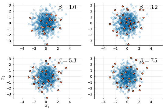
Figure 2: Samples from a DPP with ELE defined by eq. (28) and different values of $\beta$.

In figure 2, we show sampled points for different values of $\beta$, with a visible increase in repulsiveness. This apparent increase can be checked by examining the properties of the corresponding marginal kernel $\bm{K}$. One may use a repulsion index equivalent to the pair correlation function in spatial statistics. We define:

$$\rho(i,j)=1-\frac{p(i,j\subseteq\mathcal{X})}{p(i\in\mathcal{X})p(j\in\mathcal{X})}$$ (29)

which is 1 when the repulsion between $i$ and $j$ is very strong (they cannot be sampled together) and 0 when the repulsion is null (they are included “independently”). Using the definition of DPPs we obtain:

$$\rho(i,j)=\frac{K_{ij}^{2}}{K_{ii}K_{jj}}$$

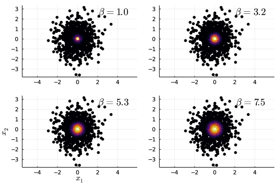
Figure 3: Repulsion index $\rho(i,j)$ for a fixed point $i$ near the center, and different values of $\beta$. The amount of repulsion is shown using a colour scale, with white for the maximum value (1) and black for the minimum. The setup is the same as in fig. 2

Figure 3 shows $\rho$ plotted using a colour scale, with $i$ fixed and set to a central point in $\Omega$. The increase in repulsiveness with $\beta$ is visible. Figure 4 shows $\rho(i,j)$ plotted as a function of the distance $\left\|\bm{x}_{i}-\bm{x}_{j}\right\|$. Since increasing $\beta$ increases the minimum size of $|\mathcal{X}|$, we cannot increase $\beta$ indefinitely while keeping $\mathbf{E}|\mathcal{X}|$ constant. This implies that there is a maximum amount of repulsiveness that can be achieved, in line with known results on continuous DPPs [9].

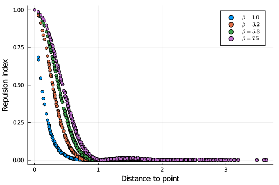
Figure 4: Repulsion index $\rho(i,j)$ for a fixed point $i$ near the center, plotted as a function of $\left\|\bm{x}_{i}-\bm{x}_{j}\right\|$. The data are the same as in fig. 3

5.4 A link with interpolation

There exists a link to interpolation (detailed recently in [15]) that we here illustrate. Suppose we want to interpolate points $((\bm{x}_{1},y_{1}),\ldots,(\bm{x}_{n},y_{n})\in(\mathbb{R}^{d}\times\mathbb{R})^{n}$ using the function

$$s(\bm{x})=\sum_{i}\alpha_{i}f(\bm{x}-\bm{x}_{i})+\sum_{k=1}^{\mathscr{P}_{\ell-1,d}}\beta_{k}p_{k}(\bm{x})$$

where $f$ is a conditionally positive function of order $\ell$, and $p_{k}$, $k=1,\ldots,\mathscr{P}_{\ell-1,d}$ is a basis for the set of polynomials of degree less or equal than $\ell-1$. For $s(x)$ to be an interpolant for the measurements $y_{1},y_{2},\ldots,y_{n}$, we need to set $\bm{\alpha}$ and $\bm{\eta}$ such that $s(\bm{x}_{i})=y_{i}$ for all $i$. The solution of this interpolation problem is then equivalent to the solution of the linear system

$$\begin{pmatrix}\bm{L}_{X}&\bm{V}_{<\ell}\\ (\bm{V}_{<\ell})^{\top}&\bm{0}\end{pmatrix}\begin{pmatrix}\bm{\alpha}\\ \bm{\beta}\end{pmatrix}=\begin{pmatrix}\bm{y}\\ \bm{0}\end{pmatrix}$$

where we recover the matrix defining the $L$-ensemble in partial projection DPPs. A DPP based on the conditional positive definite kernel $f$ will sample a good design for interpolation, since the interpolation points are selected such that the interpolation matrix is well-conditioned. See [15] for more on the topic.

6 To conclude

We have shown that DPPs can be represented as extended L-ensembles and that this representation is both useful practically and theoretically. We have deliberately kept to the discrete setting, in order to avoid the measure theory that continuous point processes require. Extending our results to the continuous setting is quite easy, and we would like to end this paper by sketching how. Defining continuous extended L-ensembles is actually easier than the traditional construction of DPPs from marginal kernels, since all that is needed is a conditionally positive definite function, to define a valid likelihood (Janossi density). There is no need to verify that the object exists, contrary to the standard approach. The next step is to use the spectral theorem along with theorem 3.1 (where the sum becomes infinite), to obtain that extended L-ensembles are mixtures of projection DPPs, from which the properties of the marginal kernel follow. We may then use the same “default” DPPs (eq. (28)) introduced here in the continuous setting. While the construction is quite straightforward, studying the properties of these DPPs is much harder and an interesting direction for future work.

Appendix A Inclusion probabilities in mixtures of projection DPPs

Here, we give formulas for inclusion probabilities valid for mixtures of projection DPPs. These formulas yield the marginal kernels of L-ensembles and partial-projection DPPs as a special case. We give a variant of a calculation in [5], appendix A.2.

Let $\bm{U}$ be a fixed orthonormal basis of $\mathbb{R}^{n}$. We assume that $\mathcal{X}$ is generated according to the following mixture process:

1. Sample indices $\mathcal{Y}\sim\mathbf{P}(\mathcal{Y})$

2. Form the projection matrix $\bm{M}=\bm{U}_{:,\mathcal{Y}}(\bm{U}_{:,\mathcal{Y}})^{\top}$

3. Sample $\mathcal{X}|\mathcal{Y}\sim|DPP|_{m}(\bm{M})$

We do not specify $\mathbf{P}(\mathcal{Y})$ for now (it may be an L-ensemble, a fixed-size L-ensemble, etc.).

Since $\mathcal{X}$ is a mixture of projection-DPPs we can write

$$\mathbf{P}(\mathcal{W}\subseteq\mathcal{X})=\mathbf{E}_{\mathcal{Y}}[\mathbf{P}(\mathcal{W}\subseteq\mathcal{X}|\mathcal{Y})]$$ (30)

where the outer expectation is over $\mathcal{Y}$, the indices of the columns of $\bm{U}$ sampled in the mixture process. Since the innermost quantity is an inclusion probability for a projection DPP, we have from lemma 1.24:

$$\mathbf{P}(\mathcal{W}\subseteq\mathcal{X}|\mathcal{Y}) =\det\left(\bm{M}_{\mathcal{W}}\right)$$

$$=\det\left(\bm{U}_{\mathcal{W},\mathcal{Y}}(\bm{U}_{\mathcal{W},\mathcal{Y}})^{\top}\right)$$

$$=\sum_{\mathcal{A}\subseteq\mathcal{Y},|\mathcal{A}|=|\mathcal{W}|}\det\left(\bm{U}_{\mathcal{W},\mathcal{A}}\right)^{2}$$

where the last line follows from the Cauchy-Binet lemma (lemma 1.1). Injecting into 30, we find:

$$\mathbf{P}(\mathcal{W}\subseteq\mathcal{X}) =\mathbf{E}_{\mathcal{Y}}\left[\sum_{\mathcal{A}\subseteq\mathcal{Y},|\mathcal{A}|=|\mathcal{W}|}\det\left(\bm{U}_{\mathcal{W},\mathcal{A}}\right)^{2}\right]$$

$$=\sum_{\mathcal{Y}}\mathbf{P}(\mathcal{Y})\sum_{\mathcal{A}\subseteq\mathcal{Y},|\mathcal{A}|=|\mathcal{W}|}\det\left(\bm{U}_{\mathcal{W},\mathcal{A}}\right)^{2}$$

$$=\sum_{\mathcal{Y},\mathcal{A}/|\mathcal{A}|=|\mathcal{W}|}\det\left(\bm{U}_{\mathcal{W},\mathcal{A}}\right)^{2}\mathbf{P}(\mathcal{Y})\bm{\mathds{I}}\{\mathcal{A}\subseteq\mathcal{Y}\}$$

$$=\sum_{\mathcal{A}/|\mathcal{A}|=|\mathcal{W}|}\det\left(\bm{U}_{\mathcal{W},\mathcal{A}}\right)^{2}\mathbf{P}(\mathcal{A}\subseteq\mathcal{Y}).$$

In the case of L-ensembles and partial projection DPPs, we can go a bit further, since the distribution of $\mathcal{Y}$ is a Bernoulli process (meaning that each element $i$ is included independently with probability $\pi_{i}$). In that case $\mathbf{P}(\mathcal{A}\subseteq\mathcal{Y})=\prod_{i\in\mathcal{A}}\pi_{i}$, and using the Binet-Cauchy lemma once again we find:

$$\mathbf{P}(\mathcal{W}\subseteq\mathcal{X}) =\sum_{\mathcal{A}/|\mathcal{A}|=|\mathcal{W}|}\det\left(\bm{U}_{\mathcal{W},\mathcal{A}}\right)^{2}\prod_{i\in\mathcal{A}}\pi_{i}$$

$$=\det\bm{U}_{\mathcal{W},:}\operatorname{diag}(\pi_{1},\ldots,\pi_{n})(\bm{U}_{\mathcal{W},:})^{\top}$$

$$=\det\bm{K}_{\mathcal{W}}$$ (31)

with $\bm{K}=\bm{U}\operatorname{diag}(\pi_{1},\ldots,\pi_{n})\bm{U}^{\top}$.

Appendix B Equivalence of extended L-ensembles and DPPs

We prove Th. 2.9 and 2.10.

Proof of Th. 2.9 .

Let $\begin{pmatrix}\bm{L};\bm{V}\end{pmatrix}$ be any NNP, and $\widetilde{\bm{L}}$, $\bm{Q}$, $\widetilde{\bm{U}}$, $\widetilde{\bm{\Lambda}}$ and $q$ be as in Definition 2.4. Let $\mathcal{X}\in\Omega$ be drawn according to the distribution:

$$\forall X\subseteq\Omega,\qquad\mathbf{P}(\mathcal{X}=X)\propto(-1)^{p}\det\begin{pmatrix}\bm{L}_{X}&\bm{V}_{X,:}\\ (\bm{V}_{X,:})^{\top}&\bm{0}\end{pmatrix}.$$ (32)

Using the generalized Cauchy-Binet formula (theorem 3.1), this can be re-written as

$$\forall X\subseteq\Omega,\qquad\mathbf{P}(\mathcal{X}=X)\propto\det(\bm{V}^{\top}\bm{V})\sum_{Y,|Y|=m-p}\det\left(\begin{bmatrix}\bm{Q}_{X,:}&\widetilde{\bm{U}}_{X,Y}\end{bmatrix}\right)^{2}\prod_{i\in Y}\widetilde{\lambda}_{i}.$$ (33)

As made precise by corollary 3.3, this equation can be interpreted from a mixture point of view. As such, the generic inclusion probability formulas of Appendix A are applicable and one obtains the result. ∎

Proof of Th. 2.10.

Given a marginal kernel $\bm{K}$, we can always rewrite its spectral factorisation in the form of Eq. (17), by grouping all the eigenvectors corresponding to the eigenvalue $1$ in $\bm{Q}$; all the remaining eigenvalues can be always represented as $\widetilde{\lambda}_{i}/(1+\widetilde{\lambda}_{i})$. ∎

Appendix C Limit of perturbed L-ensembles

There are several ways to prove this result. The more elegant ones use standard results from matrix perturbation theory. However, to avoid the introduction of additional background, we prove the result by direct calculation, i.e. we compute the limit of the marginal kernel.

We seek to evaluate

$$\bm{K}_{\varepsilon}=\bm{L}_{\varepsilon}(\bm{L}_{\varepsilon}+\bm{I})^{-1}=\bm{I}-(\bm{L}_{\varepsilon}+\bm{I})^{-1}$$

with $\bm{L}_{\varepsilon}=\bm{A}+\varepsilon^{-1}\bm{V}\bm{V}^{\top}$, which gives

$$\bm{K}_{\varepsilon}=\bm{I}-\varepsilon(\varepsilon\bm{A}+\varepsilon\bm{I}+\bm{V}\bm{V}^{\top})^{-1}.$$ (34)

We introduce a change of basis by the orthogonal matrix $\bm{R}=\begin{bmatrix}\bm{Q}&\bm{Q}_{\bot}\end{bmatrix}$ where as usual $\bm{Q}$ spans the same column space as $\bm{V}$. We apply the change of basis to $(\varepsilon\bm{A}+\varepsilon\bm{I}+\bm{V}\bm{V}^{\top})$, to find:

$$\varepsilon\bm{A}+\varepsilon\bm{I}+\bm{V}\bm{V}^{\top}=\bm{R}\begin{pmatrix}\varepsilon(\bm{P}_{1}+\bm{I})+\bm{T}&\varepsilon\bm{P}_{3}\\ \varepsilon\bm{P}_{2}&\varepsilon(\bm{P}_{4}+\bm{I})\end{pmatrix}\bm{R}^{\top}$$

where $\bm{T}=\bm{Q}^{\top}\bm{V}\bm{V}^{\top}\bm{Q}$, $\bm{P}_{1}=\bm{Q}^{\top}\bm{A}\bm{Q}$, $\bm{P}_{2}=\bm{Q}_{\bot}^{\top}\bm{A}\bm{Q}$, $\bm{P}_{3}=\bm{P}_{2}^{\top}$, $\bm{P}_{4}=\bm{Q}_{\bot}\bm{A}\bm{Q}_{\bot}^{\top}$. To find the inverse, we use the well-known formula for the inverse of block matrices. The two Schur complements are as follows:

$$\bm{S}_{a}=\varepsilon(\bm{P}_{1}+\bm{I})+\bm{T}+\varepsilon\bm{P}_{3}(\bm{P}_{4}+\bm{I})^{-1}\bm{P}_{2}=\bm{T}+\mathcal{O}(\varepsilon)$$

and

$$\bm{S}_{b}=\varepsilon(\bm{P}_{4}+\bm{I})+\varepsilon^{2}\bm{P}_{2}(\bm{T}+\mathcal{O}(\varepsilon))^{-1}\bm{P}_{3}=\varepsilon(\bm{P}_{4}+\bm{I}+\mathcal{O}(\varepsilon))$$

Injecting into eq. (34) and applying the block-matrix formula, we find:

$$\bm{R}\bm{K}_{\varepsilon}\bm{R}^{\top}=\bm{I}-\begin{pmatrix}\bm{0}&\bm{0}\\ \bm{0}&(\bm{P}_{4}+\bm{I})^{-1}\end{pmatrix}+\mathcal{O}(\varepsilon)$$

which implies:

$$\bm{K}_{\varepsilon}=\bm{Q}\bm{Q}^{\top}+\bm{Q}_{\bot}(\bm{Q}_{\bot}^{\top}\bm{A}\bm{Q}_{\bot}+\bm{I})^{-1}\bm{Q}_{\bot}^{\top}=\bm{Q}\bm{Q}^{\top}+\tilde{\bm{A}}(\tilde{\bm{A}}+\bm{I})^{-1}$$

We may now apply th. 2.9 and we are done.

References

- [1] {binproceedings}[author] \bauthor\bsnmAnari, \bfnmNima\binitsN., \bauthor\bsnmLiu, \bfnmKuikui\binitsK., \bauthor\bsnmGharan, \bfnmShayan Oveis\binitsS. O., \bauthor\bsnmVinzant, \bfnmCynthia\binitsC. and \bauthor\bsnmVuong, \bfnmThuy-Duong\binitsT.-D. (\byear2021). \btitleLog-Concave Polynomials IV: Approximate Exchange, Tight Mixing Times, and near-Optimal Sampling of Forests. In \bbooktitleProceedings of the 53rd Annual ACM SIGACT Symposium on Theory of Computing. \bseriesSTOC 2021 \bpages408–420. \bpublisherAssociation for Computing Machinery, \baddressNew York, NY, USA. \bdoi10.1145/3406325.3451091 \endbibitem
- [2] {barticle}[author] \bauthor\bsnmAvena, \bfnmL\binitsL. and \bauthor\bsnmGaudilliere, \bfnmA\binitsA. (\byear2013). \btitleOn some random forests with determinantal roots. \bjournalarXiv preprint arXiv:1310.1723. \endbibitem
- [3] {barticle}[author] \bauthor\bsnmAvena, \bfnmL.\binitsL. and \bauthor\bsnmGaudillière, \bfnmA.\binitsA. (\byear2017). \btitleTwo Applications of Random Spanning Forests. \bjournalJournal of Theoretical Probability. \bdoi10.1007/s10959-017-0771-3 \endbibitem
- [4] {barticle}[author] \bauthor\bsnmBardenet, \bfnmRémi\binitsR. and \bauthor\bsnmHardy, \bfnmAdrien\binitsA. (\byear2020). \btitleMonte Carlo with determinantal point processes. \bjournalThe Annals of Applied Probability (arXiv:1605.00361) \bvolume30 \bpages368–417. \endbibitem
- [5] {barticle}[author] \bauthor\bsnmBarthelmé, \bfnmSimon\binitsS., \bauthor\bsnmAmblard, \bfnmPierre-Olivier\binitsP.-O. and \bauthor\bsnmTremblay, \bfnmNicolas\binitsN. (\byear2019). \btitleAsymptotic Equivalence of Fixed-size and Varying-size Determinantal Point Processes. \bjournalBernoulli \bvolume25 \bpages3555–3589. \endbibitem
- [6] {barticle}[author] \bauthor\bsnmBarthelmé, \bfnmSimon\binitsS. and \bauthor\bsnmUsevich, \bfnmKonstantin\binitsK. (\byear2021). \btitleSpectral properties of kernel matrices in the flat limit. \bjournalSIAM Journal on Matrix Analysis and Applications (arXiv:1910.14067) \bvolume42 \bpages17–57. \endbibitem
- [7] {barticle}[author] \bauthor\bsnmBarthelmé, \bfnmSimon\binitsS., \bauthor\bsnmTremblay, \bfnmNicolas\binitsN., \bauthor\bsnmUsevich, \bfnmKonstantin\binitsK. and \bauthor\bsnmAmblard, \bfnmPierre-Olivier\binitsP.-O. (\byear2022). \btitleDeterminantal Point Processes in the Flat Limit. \bjournalAccepted to Bernoulli (arXiv:2107.07213). \endbibitem
- [8] {barticle}[author] \bauthor\bsnmBelhadji, \bfnmAyoub\binitsA., \bauthor\bsnmBardenet, \bfnmRémi\binitsR. and \bauthor\bsnmChainais, \bfnmPierre\binitsP. (\byear2020). \btitleA determinantal point process for column subset selection. \bjournalJournal of Machine Learning Research \bvolume21 \bpages1–62. \endbibitem
- [9] {barticle}[author] \bauthor\bsnmBiscio, \bfnmChristophe Ange Napoléon\binitsC. A. N., \bauthor\bsnmLavancier, \bfnmFrédéric\binitsF. \betalet al. (\byear2016). \btitleQuantifying repulsiveness of determinantal point processes. \bjournalBernoulli \bvolume22 \bpages2001–2028. \endbibitem
- [10] {barticle}[author] \bauthor\bsnmBorodin, \bfnmAlexei\binitsA. and \bauthor\bsnmRains, \bfnmEric M\binitsE. M. (\byear2005). \btitleEynard–Mehta theorem, Schur process, and their Pfaffian analogs. \bjournalJournal of statistical physics \bvolume121 \bpages291–317. \endbibitem
- [11] {barticle}[author] \bauthor\bsnmBurton, \bfnmRobert\binitsR. and \bauthor\bsnmPemantle, \bfnmRobin\binitsR. (\byear1993). \btitleLocal characteristics, entropy and limit theorems for spanning trees and domino tilings via transfer-impedances. \bjournalThe Annals of Probability \bpages1329–1371. \endbibitem
- [12] {barticle}[author] \bauthor\bsnmChen, \bfnmX. H\binitsX. H., \bauthor\bsnmDempster, \bfnmA. P.\binitsA. P. and \bauthor\bsnmLiu, \bfnmJ. S.\binitsJ. S. (\byear1994). \btitleWeighted finite population sampling to maximize entropy. \bjournalBiometrika \bvolume81 \bpages457–469. \endbibitem
- [13] {barticle}[author] \bauthor\bsnmCoeurjolly, \bfnmJean-François\binitsJ.-F., \bauthor\bsnmMazoyer, \bfnmAdrien\binitsA. and \bauthor\bsnmAmblard, \bfnmPierre-Olivier\binitsP.-O. (\byear2021). \btitleMonte Carlo integration of non-differentiable functions on , , using a single determinantal point pattern defined on . \bjournalElectronic Journal of Statistics \bvolume15 \bpages6228 – 6280. \bdoi10.1214/21-EJS1929 \endbibitem
- [14] {barticle}[author] \bauthor\bsnmDerezinski, \bfnmMicha\l\binitsM. and \bauthor\bsnmMahoney, \bfnmMichael W\binitsM. W. (\byear2021). \btitleDeterminantal point processes in randomized numerical linear algebra. \bjournalNotices of the American Mathematical Society \bvolume68. \endbibitem
- [15] {barticle}[author] \bauthor\bsnmFanuel, \bfnmMichaël\binitsM., \bauthor\bsnmSchreurs, \bfnmJoachim\binitsJ. and \bauthor\bsnmSuykens, \bfnmJohan AK\binitsJ. A. (\byear2020). \btitleDeterminantal Point Processes Implicitly Regularize Semi-parametric Regression Problems. \bjournalarXiv preprint arXiv:2011.06964. \endbibitem
- [16] {bphdthesis}[author] \bauthor\bsnmGautier, \bfnmGuillaume\binitsG. (\byear2020). \btitleOn sampling determinantal point processes, \btypePh.D. thesis, \bpublisherEcole Centrale de Lille. \endbibitem
- [17] {bbook}[author] \bauthor\bsnmHorn, \bfnmRoger A.\binitsR. A. and \bauthor\bsnmJohnson, \bfnmCharles R.\binitsC. R. (\byear1990). \btitleMatrix Analysis. \bpublisherCambridge University Press. \endbibitem
- [18] {barticle}[author] \bauthor\bsnmHough, \bfnmJ. Ben\binitsJ. B., \bauthor\bsnmKrishnapur, \bfnmManjunath\binitsM., \bauthor\bsnmPeres, \bfnmYuval\binitsY. and \bauthor\bsnmVirág, \bfnmBálint\binitsB. (\byear2006). \btitleDeterminantal Processes and Independence. \bjournalProbability Surveys \bvolume3 \bpages206–229. \bdoi10.1214/154957806000000078 \endbibitem
- [19] {barticle}[author] \bauthor\bsnmKlein, \bfnmDouglas J\binitsD. J. and \bauthor\bsnmRandić, \bfnmMilan\binitsM. (\byear1993). \btitleResistance distance. \bjournalJournal of mathematical chemistry \bvolume12 \bpages81–95. \endbibitem
- [20] {binproceedings}[author] \bauthor\bsnmKulesza, \bfnmAlex\binitsA. and \bauthor\bsnmTaskar, \bfnmBen\binitsB. (\byear2011). \btitlek-DPPs: Fixed-size determinantal point processes. In \bbooktitleProceedings of the 28th International Conference on Machine Learning (ICML-11) \bpages1193–1200. \endbibitem
- [21] {binproceedings}[author] \bauthor\bsnmKulesza, \bfnmAlex\binitsA. and \bauthor\bsnmTaskar, \bfnmBen\binitsB. (\byear2011). \btitlek-DPPs: fixed-size determinantal point processes. In \bbooktitleProceedings of the 28th International Conference on International Conference on Machine Learning \bpages1193–1200. \endbibitem
- [22] {barticle}[author] \bauthor\bsnmKulesza, \bfnmAlex\binitsA., \bauthor\bsnmTaskar, \bfnmBen\binitsB. \betalet al. (\byear2012). \btitleDeterminantal point processes for machine learning. \bjournalFoundations and Trends® in Machine Learning \bvolume5 \bpages123–286. \endbibitem
- [23] {barticle}[author] \bauthor\bsnmMacchi, \bfnmOdile\binitsO. (\byear1975). \btitleThe coincidence approach to stochastic point processes. \bjournalAdvances in Applied Probability \bvolume7 \bpages83-122. \bdoi10.2307/1425855 \endbibitem
- [24] {barticle}[author] \bauthor\bsnmMicchelli, \bfnmCharles A\binitsC. A. (\byear1986). \btitleInterpolation of scattered data: Distance matrices and conditionally positive definite functions. \bjournalConstructive Approximation \bvolume2 \bpages11–22. \endbibitem
- [25] {barticle}[author] \bauthor\bsnmTremblay, \bfnmNicolas\binitsN., \bauthor\bsnmBarthelme, \bfnmSimon\binitsS. and \bauthor\bsnmAmblard, \bfnmPierre-Olivier\binitsP.-O. (\byear2018). \btitleOptimized Algorithms to Sample Determinantal Point Processes. \bjournalarXiv:1802.08471 [cs, stat]. \bnotearXiv: 1802.08471. \endbibitem
- [26] {barticle}[author] \bauthor\bsnmTremblay, \bfnmNicolas\binitsN., \bauthor\bsnmBarthelmé, \bfnmSimon\binitsS. and \bauthor\bsnmAmblard, \bfnmPierre-Olivier\binitsP.-O. (\byear2019). \btitleDeterminantal Point Processes for Coresets. \bjournalJournal of Machine Learning Research \bvolume20 \bpages1–70. \endbibitem
- [27] {bbook}[author] \bauthor\bsnmWendland, \bfnmHolger\binitsH. (\byear2004). \btitleScattered data approximation \bvolume17. \bpublisherCambridge university press. \endbibitem