Hybrid A Posteriori Error Estimators for Conforming Finite Element Approximations to Stationary Convection-Diffusion-Reaction equations
Abstract
We consider the a posteriori error estimation for convection-diffusion-reaction equations in both diffusion-dominated and convection/reaction-dominated regimes. We present an explicit hybrid estimator, which, in each regime, is proved to be reliable and efficient with constants independent of the parameters in the underlying problem. For convection-dominated problems, the norm introduced by Verfürth [33] is used to measure the approximation error. Various numerical experiments are performed to demonstrate the robustness of the hybrid estimator; show that the hybrid estimator is more accurate than the explicit residual estimator and is less sensitive to the size of reaction, even though both of them are robust.
1 Introduction
The a posteriori error estimation has been an indispensable tool in handling computationally challenging problems. For elliptic partial differential equations (PDEs) consisting of terms characterizing diffusion, reaction and convection, the solution may display a strong interface singularity, interior or boundary layers, etc., due to discontinuous coefficients or terms in significantly different scales, etc. Consequently, it is a challenging task to design a general a posteriori error estimator that is accurate and robust enough to resolve local behaviors of the exact solution without spending much computational resource.
Explicit residual estimators are directly related to the error and have been well-studied since 1970s (cf. [7, 6, 30, 9, 23, 32, 31, 33, 29]). They are easy to compute, applicable to a large class of problems, valid for higher order elements, etc. More importantly, robust residual estimators have been proposed for various problems. For diffusion problems with discontinuous coefficient, [9, 23] established robustness with respect to coefficient jump under the monotonicity or quasi-monotonicity assumption of the diffusion coefficient. For singularly perturbed reaction-diffusion problems, Verfürth [32] pioneered a residual estimator that is robust with respect to the size of reaction. For convection-dominated problems, it is still under debate on how to choose a suitable norm to measure the approximation error (cf. [28, 31, 24, 25, 33, 26]). Sangalli [25, 26] proposed a norm incorporating the standard energy norm and a seminorm of order and developed the a posteriori error analysis in the one-dimensional setting. Verfürth [33] introduced a norm incorporating the standard energy norm and a dual norm of the convective derivative. With respect to this norm, the explicit residual estimator in [33] was proved to be robust. Moreover, it was shown in [29] that the framework of residual estimators is applicable for various stabilization schemes. Those developments make residual estimators competitive when dealing with challenging problems. One drawback, however, is that residual estimators tend to overestimate the true error by a large margin (cf. [14, 10]). This calls for the need of an estimator as general as the residual estimator but with improved accuracy.
Recovery-based estimators, e.g., the Zienkiewicz–Zhu (ZZ) estimator and its variations (cf. [34, 35, 27, 13, 21, 8, 18], etc.), are quite popular in the engineering community. However, unlike residual estimators, the robustness of those estimators with respect to issues like coefficient jump, dominated convection or reaction, etc., has not been emphasized or studied in detail yet (cf. [22]). On coarse meshes, it is known that ZZ-type estimators are in general unreliable, and counterexamples can be easily constructed where the estimator vanishes but the true error is large (cf. [3, 10]). For linear elements, [18, 17] adds two additional terms (one of them is the element residual) to the ZZ estimator to ensure reliability on coarse meshes. For higher order elements, however, a straightforward extension of the original ZZ estimator [34, 35] usually fails and developing a viable estimator is nontrivial. For example, Bank, Xu, and Zheng in [8] recently introduced a recovery-based estimator for Lagrange triangular elements of degree , and their estimator requires recovery of all partial derivatives of order instead of the gradient.
Recently, the so-called hybrid estimator was introduced in [10, 12] for diffusion problems with discontinuous coefficients. The explicit hybrid estimator shares all advantages of the robust residual estimator [9, 23] and numerical results indicate that the hybrid estimator is more accurate than the residual estimator (cf. [10]). This opens a door of finding an alternative of the residual estimator with improved accuracy. Thus one may ask if it is possible to construct hybrid estimators for more general problems and if the hybrid estimator is still more accurate than the residual estimator.
In this manuscript, we introduce the hybrid estimator as well as flux recoveries for convection-diffusion-reaction equations. In diffusion-dominated regime, the flux recovery as well as the hybrid estimator is a natural extension of the one in [10]. In convection/reaction-dominated regime, the flux recovery in each element depends on the size of diffusion. Roughly speaking, in elements with resolved diffusion (see Section 4.2.1), the recovered flux is same to the diffusion-dominated case; in elements where diffusion is not resolved, inspired in part by the method of Ainsworth and Vejchodský [4, Section 3.4], the recovered flux is defined piecewisely in each element (see Section 4.2.2). The hybrid estimator in the convection/reaction-dominated regime is analogously defined as in [10] with proper weights from [33]. In each regime, we prove that the hybrid estimator is equivalent to the robust residual estimator (for example, [33] for the convection/reaction-dominated regime) and then the robustness follows immediately from that of the residual estimator. The hybrid estimator is explicit and valid for higher order elements. Various numerical results show that, compared to the explicit residual estimator, the hybrid estimator is more accurate and the corresponding effectivity index is less sensitive to the size of reaction.
The rest of the manuscript is organized as follows. The model problems and finite element discretizations are introduced in Section 2. Section 3 collects results on robust residual estimators. After the flux recovery presented in Section 4, the hybrid estimator is defined in Section 5 along with robust a posteriori error estimates. Section 6 gives the proof of the local equivalence between the residual estimator and the hybrid estimator. Numerical results are shown in Section 7.
2 Problems and Discretizations
Let be a polygonal domain in () with Lipschitz boundary consisting of two disjoint components and . By convention, assume that . Consider the stationary convection-diffusion-reaction equation:
| (1) |
with , for almost all and for some constant . Assume that:
-
(A1)
and ;
-
(A2)
there are two constants and , independent of , such that
-
(A3)
and contains the inflow boundary
Depending on the magnitude of the (with respect to and ), two regimes are studied in this paper:
-
1.
diffusion-dominated regime: there exists a constant such that
-
2.
convection/reaction-dominated regime: for a constant . This is the so-called singularly perturbed problem.
Let
Define the bilinear form on by
where denotes the inner product on set and the subscript is omitted when . The norm on is denoted by .
The weak formulation of (1) is to find such that
| (2) |
It follows from integration by parts and the assumptions in (A2) and (A3) that, for any ,
| (3) |
where denotes the unit outward vector normal to . The energy norm induced by is defined by
where denotes the energy norm over and the subscript is omitted when .
Let be a regular triangulation of (see, e.g., [15]). Define the following sets associated with the triangulation :
For a simplex , denote by and its measure and diameter, respectively. Denote by the inradius of . The shape regularity of the triangulation requires the existence of a generic constant such that
| (4) |
holds true for each mesh in the adaptive mesh refinement procedure.
We associate each with a unit normal , which is chosen as the unit outward normal if . Denote by and the two elements sharing such that the unit outward normal of on coincides with . For , let denote the element next to sharing in common. Let be the union of elements adjacent to and be the union of elements that share at least one face with . Unless otherwise stated, always denotes the unit outward normal vector on .
For , let denote the set of polynomials of degree at most on and denote the -projection onto . Define the conforming finite element space of order () by
For each , the Raviart-Thomas space of index () is
The projected data and are defined by
respectively.
The standard finite element approximation for problem (1) is to find such that
| (5) |
In the case that the convection is dominant, one often adds a stabilization term along the convective direction. For example, the so-called SUPG method in [19] is to find such that
| (6) |
where the stabilized bilinear and linear forms are given by
for all and
for all , respectively. Here, the stabilization parameters are nonnegative and satisfy
To measure the convective derivative, the following dual norm was used in [33]:
where is in the dual space of and denotes the duality pairing. Following [33], the dual norm will be combined with the energy norm to measure the approximation error in the convection-dominated regime.
To keep the exposition simple, we ignore data oscillation in coefficients by further assuming that for each , , , and are constants. The algorithm and analysis remain valid without this assumption if we replace those quantities with their proper projections and add the corresponding oscillation error in the estimates.
Define
For diffusion-dominated case, we are interested in the case where may be discontinuous and the hybrid estimator is robust with respect to the discontinuity. For convection/reaction-dominated case (), we design a hybrid estimator that is robust with respect to and in appropriate norms.
3 Residual Estimator
Let be the numerical flux, then the element residual and the flux jump across are given by
| (7) |
and
| (8) |
respectively. For , define the weight as below
| (9) |
The residual estimator is defined by
| (10) |
Note that for diffusion-dominated problems, the is a simple extension of the one in [9] or [23] for pure diffusion problems; for convection/reaction-dominated problems, the is introduced by Verfürth in [33]. In fact, is same to the weight defined in [33, Eq.(3.4)]. Here, is additional weight needed for convection/reaction-dominated problems.
Remark 3.1.
In the remainder of this section, we will discuss reliability and efficiency bounds of the estimator .
3.1 Convection/reaction-dominated regime
The global reliability and efficiency bounds of the were established by Verfürth in [33, Theorem 4.1]. The reliability and efficiency constants are uniform with respect to and . For reader’s convenience, they are cited below.
Define the data oscillation on by
Theorem 3.1.
Here and thereafter, we will use with or without subscripts to denote a generic nonnegative constant, possibly different at different occurrences, that is independent of any mesh-size and the problem parameters: either and for dominant convection/reaction, or for the dominant diffusion, but may depend on the shape parameter of mesh and on the polynomial degree .
The reaction-dominated diffusion problem, i.e., with , , and , corresponds to the singularly perturbed reaction-diffusion equation:
| (11) |
The assumptions in Section 2 are fulfilled with . For the finite element approximation in (5) to the problem in (11), the residual estimator in (10) is proved by Verfürth in [32] to be globally reliable (see Theorem 3.1); moreover, it is not only globally but also locally efficient.
3.2 Diffusion-dominated regime
For the diffusion-dominated case, following the pure diffusion case in [9] or [23], this section establishes global reliability and local efficiency of the estimator . These estimates are proved to be robust in terms of the discontinuity of the diffusion coefficient .
To this end, let be the exact solution in (2) and be the finite element solution in (5). An alternative and often used expression of the element residual in (7) is given in terms of the true error and the data oscillation:
| (12) |
Theorem 3.3.
Under the monotonicity assumption [9, Hypothesis 2.7] of , the residual estimator satisfies the following reliability estimate: there exists a positive constant such that
Proof.
Let . To prove the reliability bound, according to [9], it suffices to derive an estimate of the error in the form below:
| (13) | ||||
Theorem 3.4.
There exists a constant such that
4 Flux Recovery
We show in this section how to recover a suitable flux in , denoted by , such that the resulting hybrid estimator is robust. Same to [10], the recovered normal component on is defined as a weighted average of normal components:
| (14) |
where is the element sharing and the average weight is given by
For the diffusion-dominated case, is defined in (15). For convection/reaction-dominated case, the form of in an element depends on the size of the element . Its construction remains the same as in (15) if is relatively small. Otherwise, it is essentially the numerical flux with transitional regions to be in .
4.1 Diffusion-dominated regime
4.2 Flux recovery in convection/reaction-dominated regime
In the case that is a constant, the weight is . This may be simplified as for all if the size of each element is close to sizes of its neighboring elements. With given normal components of the recovered flux on each face, the construction on each element depends on the size of .
4.2.1 Flux recovery in with
On element with , the recovered flux is simply defined as in (15).
Remark 4.1.
The case of absent reaction corresponds to , or equivalently, . Consequently, holds true for all . Therefore, the recovered flux in each element is given by (15).
4.2.2 Flux recovery in with
For simplicity, here we restrict our attention to . For the three dimensional case, the partition of the tetrahedron follows [1] and the piecewise definition of the recovered flux shares similar idea as the two dimensional case.
For element with , we will define the recovered flux piecewisely. To this end, as in [4], is first partitioned into a triangle and three trapezoids illustrated in Figure 2. The edges of the triangle are parallel to corresponding edges of and the distance between each pair of parallel edges from to is equal to . Each trapezoid is further partitioned into a rectangle and two triangles. Figure 2 illustrates the partition of the trapezoid on into a rectangle, denoted by , and two triangles, denoted by and , respectively.


With the above partition of , to guarantee , its normal component on element interfaces of is defined to be that of the numerical flux. On the triangle , the recovered flux is chosen to be the numerical flux:
| (18) |
On each rectangle, equals to plus a correction from an edge of to its parallel edge of such that the normal components of is equal to the preassigned normal components on these two edges. Specifically, let and be a unit vector normal to (see Figure 2), the recovered flux is given by:
| (19) |
where and are local coordinates of point .
On each triangle or , is defined similar to that in (15) (see [10]):
| (20) |
where denotes the unit outward normal for ,
| (21) |
and the space is defined as in (17).
Inside , it is easy to verify that the normal component of is continuous over and , whose value is actually equal to that of . Hence . On , the normal component of is always given by . Therefore, we see that .
5 Hybrid Estimator
The hybrid estimator is defined as
| (22) |
where is defined in (9) and the modified element residual is given by
| (23) |
To establish the reliability and the efficiency of the hybrid estimator , we use the following local equivalence between and , which is proved in Section 6.
Lemma 5.1.
Thanks to the equivalence result in Lemma 5.1, the reliability and efficiency of the hybrid estimator follow immediately from the corresponding results of the residual estimator .
Theorem 5.1.
In the diffusion-dominated regime, let be the exact solution of (2) and be the finite element solution in (5). For the hybrid estimator defined in (22), there exists a constant such that
Furthermore, under the monotonicity assumption [9, Hypothesis 2.7] of , there exists a positive constant such that
Proof.
Theorem 5.2.
For the singularly perturbed reaction-diffusion equation (11), in addition to the global efficiency bound in Theorem 5.2, satisfies a local efficiency bound as a counterpart of Theorem 3.2.
Theorem 5.3.
Remark 5.1.
For the singularly perturbed reaction-diffusion equation (11), in addition to the robust residual estimator in [32], other types of estimators have been proposed over the years. A general recovery-based estimator was proposed in [12] based on projecting the numerical flux onto an -conforming space. The global -projection, however, may be regarded computationally expensive by some researchers. A series of estimators based on flux equilibration were explored in [2, 4, 5], where the estimators yield guaranteed upper bounds of the true error. The flux equilibration techniques in [4, 5] require solving local least square problems associated with each vertex patch and only piecewise linear finite element approximations were discussed. For diffusion equations, flux equilibration was discussed for higher order elements in [11]. For convection-diffusion-reaction equations, a flux equilibration procedure for linear elements was proposed in [1], where the resulting estimator yields a guaranteed upper bound of the true error. The results in [1] were derived under the assumption and the robustness was restricted to the special case of vanishing reaction i.e., .
6 Proof of Lemma 5.1
In diffusion-dominated regime, the proof of (24) is the same as that of [10, Theorem 4.2]. In convection/reaction-dominated regime, the proof of (24) is more complicated. We first prove the upper bound of (24) in Section 6.1. The lower bound of (24) will be justified in Section 6.2.
6.1 Upper bound
The proof of the upper bound is analogous to that in [10, Theorem 4.2], which is essentially based on the proof of local efficiency of residual estimator using properly chosen bubble functions.
Let be the standard element bubble function on and be modified face bubble function associated with defined in [33]. Unlike standard bubble functions that only depend on the geometry of the mesh, the modified face bubble function also involves and in order to fulfill the estimates in (25). It is known from [33, Lemma 3.6] that
| (25) |
6.2 Lower bound
In this section, we prove the lower bound in (24) in the convection/reaction-dominated regime. That is, for any , there exists a positive constant independent of , , and such that
| (27) |
This is proceeded in two cases: (i) and (ii) .
Proof in Case (i).
In this case, the inequality and (4) give
which implies the weight is independent of , , and . Hence, to show the validity of (27), it suffices to prove that
| (28) |
To this end, note first that and that the recovered flux defined in (15) satisfies
| (29) |
which, together with [10, Lemma 4.1] and the triangle inequality, implies
| (30) | ||||
To bound the modified element residual in (23), by (29) we have
which yields
| (31) |
Now, (28) is a direct consequence of (30), (31), and the following bound
which follows from the divergence theorem and the triangle and the Cauchy-Schwarz inequalities that
Proof in Case (ii).
When , the fact that implies
| (32) |
To prove (27), it suffices to show that
| (33) |
To this end, we first estimate . Note that
for all , where are local coordinates in , and
| (34) |
Define at this moment . A straightforward calculation gives
| (35) |
The estimate of for and is analogous to Case (i). It follows from (34), the fact that , and the Cauchy-Schwarz inequality that
| (36) |
which, together with [10, Lemma 4.1], implies
for all . Combining with (35) gives
| (37) |
It remains to estimate . By (23) and the triangle inequality, we have
| (38) |
It follows from the definition of that
for all . A straightforward calculation yields
which, together with (36), implies
| (39) |
∎
7 Numerical Experiments
In numerical experiments, we consider the singularly perturbed reaction-diffusion problem in (11). Here the domain is chosen as . The initial mesh in the adaptive mesh refinement consists of congruent squares, each of which is partitioned into two triangles connecting bottom-left and top-right corners. As in [16, 20, 10], we use Dörfler’s marking strategy [16] with (cf. [10, Eq.(5.1)]). The newest-vertex bisection [27] is used in the refinement. For the finite element discretization, conforming element is used in all examples. The exact error is denoted by . “DOFs” denotes the degrees of freedom and “eff-ind” denotes the effectivity index, namely, either or .
Remark 7.1.
The performance of the hybrid estimator for diffusion-dominated problems can be seen from the numerical results in [10].
7.1 Test Problem 1
We first consider an example as in [4, Example 1], where the solution is smooth but, as pointed out in [4], non-robust estimators do not perform well . The exact solution is chosen as
and the data is . The aim of this example is to numerically show that the hybrid estimator is more accurate than the residual estimator and to demonstrate that is less sensitive with respect to the variation of .
7.1.1 Effectivity with respect to
On a fixed uniform mesh composed of isosceles right triangles, we vary and investigate the change of effectivity index for each estimator. Numerical results are collected in Table 1 for different choices of . It is easily seen from Table 1 that the hybrid estimator is more accurate and than the residual estimator . When changes gradually from to , the effectivity indices for remain close to , while the effectivity indices for increase significantly from to , by a factor of . This implies that, compared to the explicit residual estimator , the hybrid estimator is less sensitive to the size of reaction.
| 1E-5 | 1E-4 | 5E-4 | 1E-3 | 5E-3 | 1E-2 | 5E-2 | 1E-1 | 1 | 10 | 100 | |
|---|---|---|---|---|---|---|---|---|---|---|---|
| 0.66 | 0.66 | 0.93 | 1.21 | 2.22 | 2.81 | 4.83 | 5.58 | 5.57 | 5.56 | 5.56 | |
| 0.80 | 0.84 | 1.09 | 1.35 | 1.20 | 1.28 | 1.38 | 1.38 | 1.36 | 1.36 | 1.36 |
7.1.2 Effectivity during adaptive mesh refinement
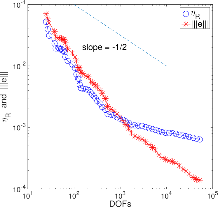
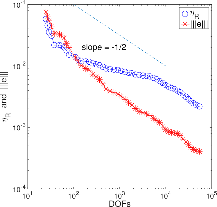
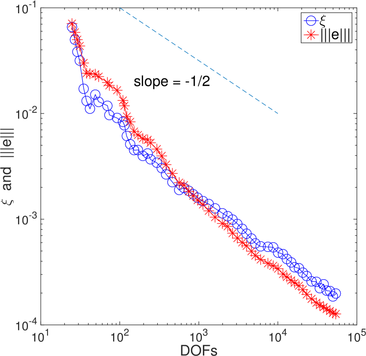
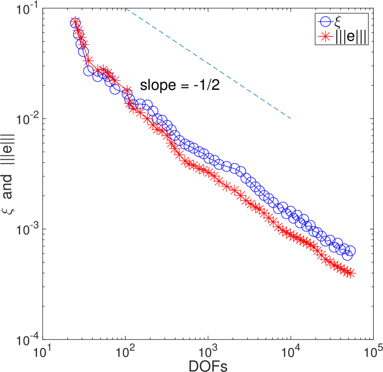
In this section, for each fixed , we investigate the effectivity of each estimator during adaptive mesh refinement.
The numerical results for the residual estimator are shown in Figure 3 – 4 for different . (The result for or is quite similar to and is thus not shown here.) It is obviously seen that the effectivity of strongly depends on the relation between and mesh-size. Hence even though theoretically the constants in the a posteriori error estimates for are independent of , the practical performance does display a significant difference for different choices of . This is because the theoretical results can only provide lower and upper bounds of , i.e., an interval that lies in, and the exact value may vary in such a (possibly large) interval. In this case, the size of this interval could be quite large even though it is independent of .
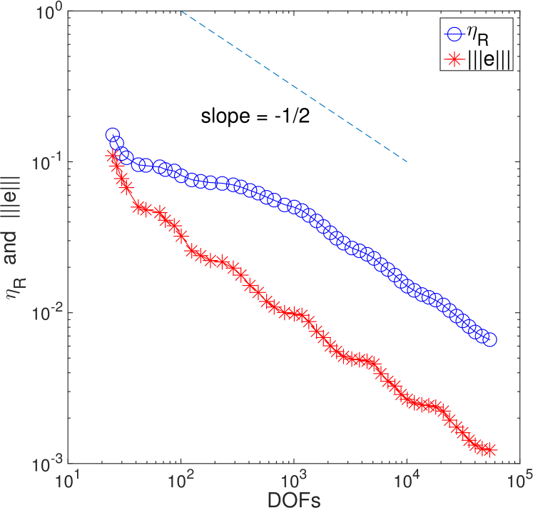
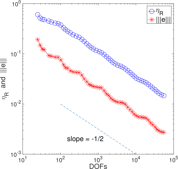
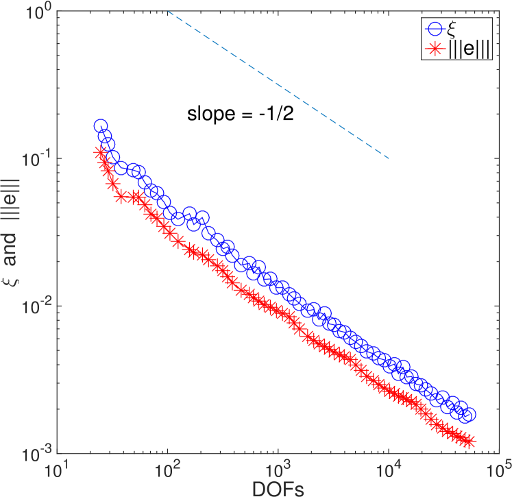
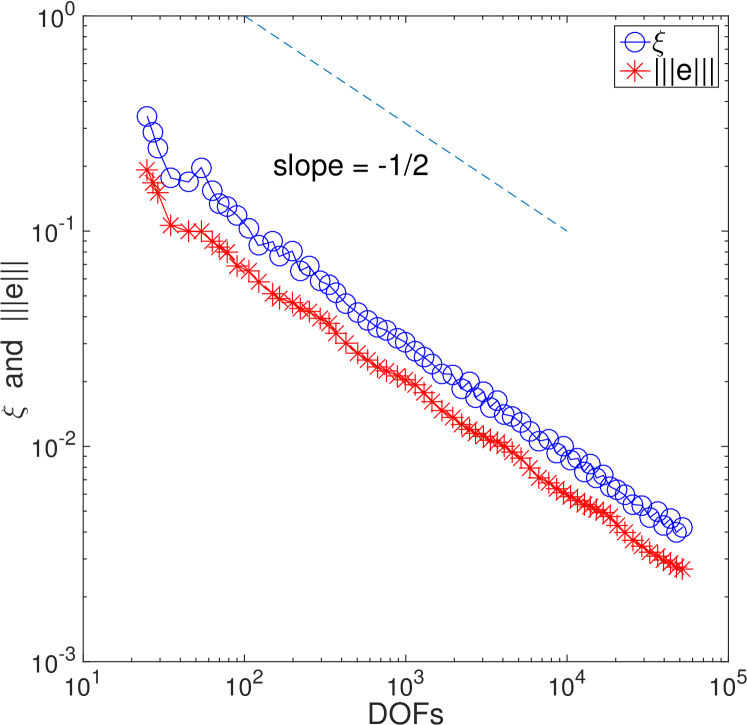
The numerical results for the hybrid estimator are shown in Figure 5 – 6 for different . Unlike , numerical results indicate that does not have much influence on the effectivity of during the adaptive mesh refinement. Therefore, we see that the hybrid estimator is indeed less sensitive than the residual estimator with respect to .
7.2 Test Problem 2
Test problem 2 has and the exact solution
which displays boundary layers along and .
We perform adaptive mesh refinement with stopping criterion and compare the results obtained using and .
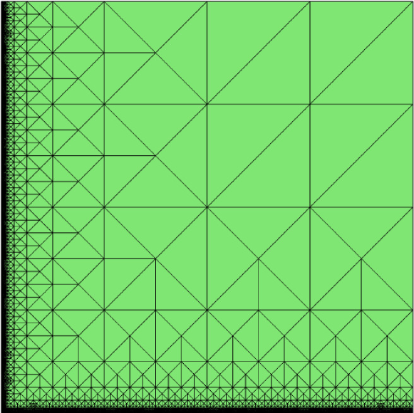
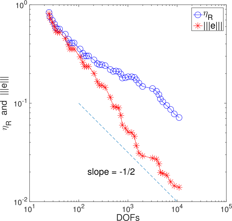
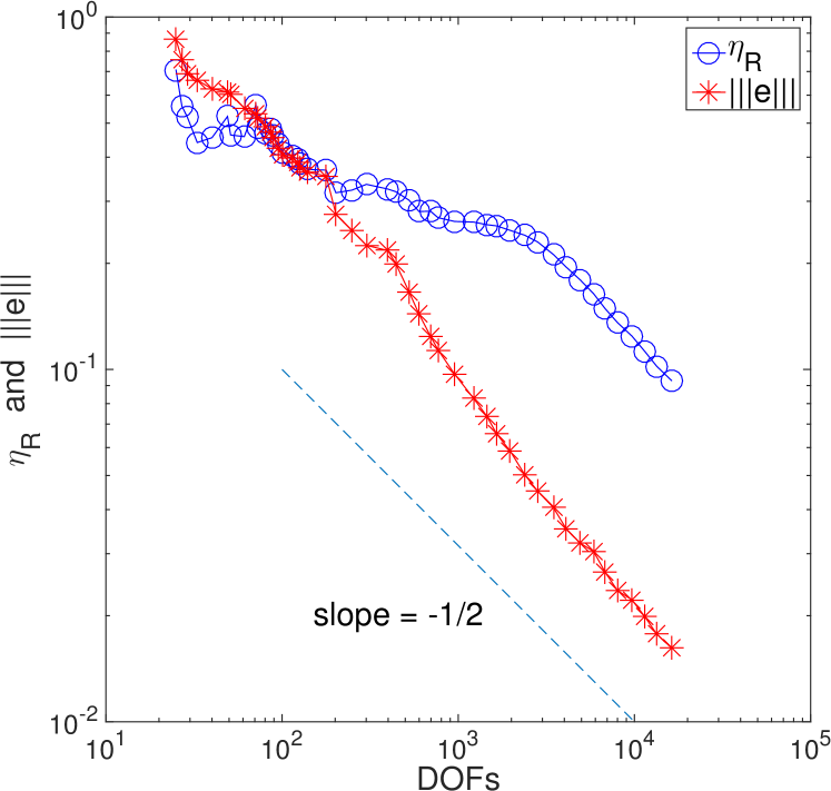
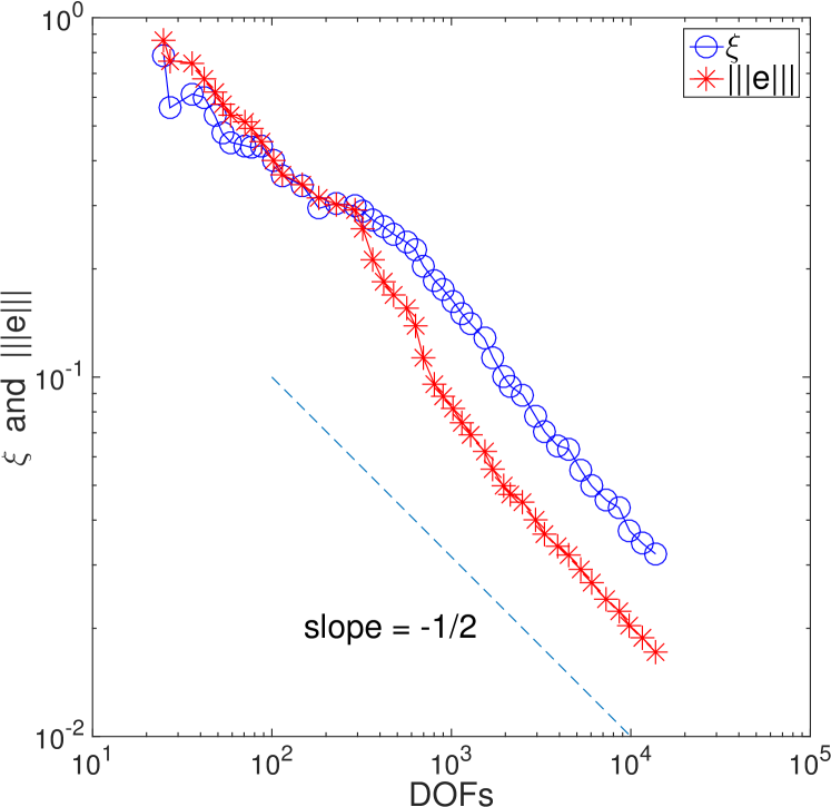
The mesh generated by is shown in Figure 7 (left), where major refinements are along the boundary layers. From Table 2, it is easy to see that the residual estimator is less accurate than the hybrid estimator. Figure 8 again shows that the effectivity index of varies more widely than that of during the mesh refinement procedure. The robustness of as well as can be seen from Figure 8 as the optimal error decay rate is observed on very coarse meshes (DOFs100).
| estimator | DOFs | eff-ind | |
|---|---|---|---|
| 10987 | 9.8E-2 | 5.11 | |
| 9383 | 9.9E-2 | 1.80 |
7.3 Test Problem 3
The exact solution is chosen as
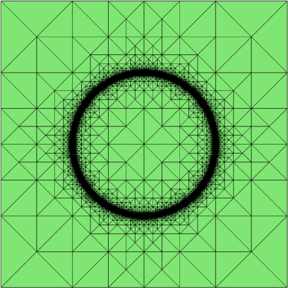
which displays an interior layer on a circle with radius .
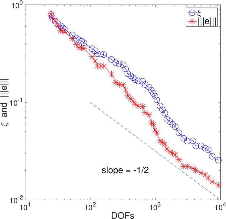
The stopping criterion for the adaptive mesh refinement is chosen as . The mesh generated by is shown in Figure 7 (right), where major refinements are along the interior layer. In terms of accuracy or effectivity, from Table 3 and Figure 9, the same conclusion can be drawn as in Example 2: the residual estimator is less accurate than the hybrid estimator and its effectivity index varies more widely during the adaptive mesh refinement. Figure 9 shows that the error starts to decay in optimal rate on very coarse meshes (DOFs100), which demonstrates the robustness of the estimators and .
| estimator | DOFs | eff-ind | |
|---|---|---|---|
| 16217 | 9.2E-3 | 5.74 | |
| 13664 | 9.8E-3 | 1.88 |
References
- [1] M. Ainsworth, A. Allendes, G. R. Barrenechea, and R. Rankin. Fully computable a posteriori error bounds for stabilised FEM approximations of convection–reaction–diffusion problems in three dimensions. International Journal for Numerical Methods in Fluids, 73(9):765–790, 2013.
- [2] M. Ainsworth and I. Babuška. Reliable and robust a posteriori error estimation for singularly perturbed reaction-diffusion problems. SIAM Journal on Numerical Analysis, 36(2):331–353, 1999.
- [3] M. Ainsworth and J.T. Oden. A Posteriori Error Estimation in Finite Element Analysis, volume 37. John Wiley & Sons, 2000.
- [4] M. Ainsworth and T. Vejchodský. Fully computable robust a posteriori error bounds for singularly perturbed reaction–diffusion problems. Numerische Mathematik, 119(2):219–243, 2011.
- [5] M. Ainsworth and T. Vejchodský. Robust error bounds for finite element approximation of reaction–diffusion problems with non-constant reaction coefficient in arbitrary space dimension. Computer Methods in Applied Mechanics and Engineering, 281:184–199, 2014.
- [6] I. Babuška and A. Miller. A feedback element method with a posteriori error estimation: Part i. the finite element method and some basic properties of the a posteriori error estimator. Computer Methods in Applied Mechanics and Engineering, 61(1):1–40, 1987.
- [7] I. Babuška and W. C. Rheinboldt. Error estimates for adaptive finite element computations. SIAM Journal on Numerical Analysis, 15(4):736–754, 1978.
- [8] R. Bank, J. Xu, and B. Zheng. Superconvergent derivative recovery for Lagrange triangular elements of degree p on unstructured grids. SIAM Journal on Numerical Analysis, 45(5):2032–2046, 2007.
- [9] C. Bernardi and R. Verfürth. Adaptive finite element methods for elliptic equations with non-smooth coefficients. Numerische Mathematik, 85(4):579–608, 2000.
- [10] D. Cai and Z. Cai. A hybrid a posteriori error estimator for conforming finite element approximations. Computer Methods in Applied Mechanics and Engineering, 339:320 – 340, 2018.
- [11] D. Cai, Z. Cai, and S. Zhang. Robust equilibrated a posteriori error estimator for higher order finite element approximations to diffusion problems. Numerische Mathematik, 144(1):1–21, 2020.
- [12] Z. Cai and S. Zhang. Flux recovery and a posteriori error estimators: conforming elements for scalar elliptic equations. SIAM Journal on Numerical Analysis, 48(2):578–602, 2010.
- [13] C. Carstensen. All first-order averaging techniques for a posteriori finite element error control on unstructured grids are efficient and reliable. Mathematics of Computation, 73(247):1153–1165, 2004.
- [14] C. Carstensen and C. Merdon. Estimator competition for poisson problems. Journal of Computational Mathematics, pages 309–330, 2010.
- [15] P. Ciarlet. The Finite Element Method for Elliptic Problems. Society for Industrial and Applied Mathematics, 2002.
- [16] W. Dörfler. A convergent adaptive algorithm for poisson’s equation. SIAM Journal on Numerical Analysis, 33(3):1106–1124, 1996.
- [17] F. Fierro and A. Veeser. A posteriori error estimators, gradient recovery by averaging, and superconvergence. Numerische Mathematik, 103(2):267–298, 2006.
- [18] F. Fierro and A. Veeser. A safeguarded Zienkiewicz-Zhu estimator. In Numerical Mathematics and Advanced Applications, pages 269–276. Springer, 2006.
- [19] L.P. Franca, S.L. Frey, and T.J.R. Hughes. Stabilized finite element methods: I. application to the advective-diffusive model. Computer Methods in Applied Mechanics and Engineering, 95(2):253–276, 1992.
- [20] P. Morin, R.H. Nochetto, and K.G. Siebert. Convergence of adaptive finite element methods. SIAM Review, 44(4):631–658, 2002.
- [21] A. Naga and Z. Zhang. The polynomial-preserving recovery for higher order finite element methods in 2D and 3D. Discrete and Continuous Dynamical Systems Series B, 5(3):769, 2005.
- [22] J.S. Ovall. Two dangers to avoid when using gradient recovery methods for finite element error estimation and adaptivity. Technical report, Technical report 6, Max-Planck-Institute fur Mathematick in den Naturwissenschaften, Bonn, Germany, 2006.
- [23] M. Petzoldt. A posteriori error estimators for elliptic equations with discontinuous coefficients. Advances in Computational Mathematics, 16(1):47–75, 2002.
- [24] G. Sangalli. A robust a posteriori estimator for the residual-free bubbles method applied to advection-diffusion problems. Numerische Mathematik, 89(2):379–399, 2001.
- [25] G. Sangalli. A uniform analysis of nonsymmetric and coercive linear operators. SIAM Journal on Mathematical Analysis, 36(6):2033–2048, 2005.
- [26] G. Sangalli. Robust a-posteriori estimator for advection-diffusion-reaction problems. Mathematics of Computation, 77(261):41–70, 2008.
- [27] E. G. Sewell. Automatic generation of triangulations for piecewise polynomial approximation. PhD thesis, Purdue University, West Lafayette, IN, 1972.
- [28] M. Stynes. Steady-state convection-diffusion problems. Acta Numerica, 14:445–508, 2005.
- [29] L. Tobiska and R. Verfürth. Robust a posteriori error estimates for stabilized finite element methods. IMA Journal of Numerical Analysis, 35(4):1652–1671, 2015.
- [30] R. Verfürth. A posteriori error estimation and adaptive mesh-refinement techniques. Journal of Computational and Applied Mathematics, 50(1):67 – 83, 1994.
- [31] R. Verfürth. A posteriori error estimators for convection-diffusion equations. Numerische Mathematik, 80(4):641–663, 1998.
- [32] R. Verfürth. Robust a posteriori error estimators for a singularly perturbed reaction-diffusion equation. Numerische Mathematik, 78(3):479–493, 1998.
- [33] R. Verfürth. Robust a posteriori error estimates for stationary convection-diffusion equations. SIAM Journal on Numerical Analysis, 43(4):1766–1782, 2005.
- [34] O.C. Zienkiewicz and J.Z. Zhu. A simple error estimator and adaptive procedure for practical engineerng analysis. International Journal for Numerical Methods in Engineering, 24(2):337–357, 1987.
- [35] O.C. Zienkiewicz and J.Z. Zhu. The superconvergent patch recovery and a posteriori error estimates. part 1: The recovery technique. International Journal for Numerical Methods in Engineering, 33(7):1331–1364, 1992.