eq
| (0.1) |
Spectral recovery of binary censored block models††thanks: A full version of the paper can be accessed at arXiv:2107.06338
Abstract
Community detection is the problem of identifying community structure in graphs. Often the graph is modeled as a sample from the Stochastic Block Model, in which each vertex belongs to a community. The probability that two vertices are connected by an edge depends on the communities of those vertices. In this paper, we consider a model of censored community detection with two communities, where most of the data is missing as the status of only a small fraction of the potential edges is revealed. In this model, vertices in the same community are connected with probability while vertices in opposite communities are connected with probability . The connectivity status of a given pair of vertices is revealed with probability , independently across all pairs, where . We establish the information-theoretic threshold , such that no algorithm succeeds in recovering the communities exactly when . We show that when , a simple spectral algorithm based on a weighted, signed adjacency matrix succeeds in recovering the communities exactly.
While spectral algorithms are shown to have near-optimal performance in the symmetric case, we show that they may fail in the asymmetric case where the connection probabilities inside the two communities are allowed to be different. In particular, we show the existence of a parameter regime where a simple two-phase algorithm succeeds but any algorithm based on the top two eigenvectors of the weighted, signed adjacency matrix fails.
††Emails: sdhara@mit.edu, julia.gaudio@northwestern.edu, elmos@mit.edu, csandon@mit.edu††Acknowledgement: S.D., E.M and C.S. are partially supported by Vannevar Bush Faculty Fellowship ONR-N00014-20-1-2826. E.M. and C.S. are partially supported by NSF award DMS-1737944. E.M. is partially supported by Simons Investigator award (622132) and by ARO MURI W911NF1910217. Part of this work was completed while J.G. was at the Department of Mathematics, Massachusetts Institute of Technology.1 Introduction
The problem of detecting community structure is an important question in the study of networks. The canonical formulation of this problem is made via the stochastic block model (SBM), where each vertex is a member of one of communities, and vertices create an edge independently based on their latent community assignments. The objective is to recover the latent community assignments based on the observed network. One may be interested in exact, partial, or weak recovery. When the average degree scales as , such that the graph is connected with high probability, one is often interested in recovering the community assignments exactly. Previous literature gives us precise characterization on when the exact recovery problem is efficiently solvable and when it is information theoretically impossible [ABH16, MNS16, AS15, Krzakala2013]. See the survey [A18] for an overview.
Popular approaches for community detection in the stochastic block model include spectral algorithms and semidefinite programming. Given the adjacency matrix representation of the graph, spectral algorithms use properties of the eigenvalues and eigenvectors of the matrix in order to infer the communities [Newman2013, Chin2015, Yun2014, Abbe2020]. Other approaches are based on the “non-backtracking” matrix of the graph [Krzakala2013, Bordenave2015]. Semidefinite programming approaches [Montanari2016, Hajek2016, Hajek2016b] are typically a relaxation of the maximum likelihood estimator, which is NP-hard to compute directly.
In this paper, we study the community detection problem when we only have partial knowledge about the graph. The information about the status of an edge between each pair of vertices is censored independently, i.e., an edge between a pair of vertices can be present, absent or censored. A precise description is given below in Definition 2.1. This model is referred to as the Censored Stochastic Block Model (CSBM). Abbe, Bandeira, Bracher, and Singer [ABBS14] were the first to address the exact recovery problem on CSBM when the within community edge probability and the between community edge probability satisfy . They show that the Maximum Likelihood Estimator (MLE) achieves exact recovery up to the information theoretic threshold. However, the MLE turns out to be equivalent to the Max-Cut problem and is thus NP-hard to compute. For this reason, [ABBS14] considered the Semidefinite Programming (SDP) relaxation which was shown to work in a certain regime. Later, Hajek, Wu, and Xu [Hajek2015, Hajek2016] proved that, under this set up, the SDP relaxation actually works up to the information theoretic threshold.
The impressive line of work above leaves an important question open: what families of algorithms achieve exact recovery for the CSBM up to the information theoretic threshold? Given that semidefinite programming is less efficient than spectral approaches, the main question of this paper is:
Question:
Are spectral algorithms information theoretically optimal for exact recovery of CSBMs?
It is important to note here the difference between purely spectral algorithms and algorithms that combine spectral algorithms with additional clean-up procedures. The results on exact recovery for the standard block model in [ABH16, MNS16] used spectral algorithms as the first step in a two stage procedure. In the usual uncensored stochastic block model, Abbe, Fan, Wang, and Zhong [Abbe2020] recently showed that the spectral algorithm is optimal, without need for a clean-up stage. It was not immediately clear whether the same would be true for the censored version that we consider, since observations are ternary (present, absent, censored) rather than binary (present, absent).
We are also interested in answering the spectral question in a more general setup than what was previously considered. First, previous results focused on the case that which ensures that a present edge carries the same relative information as an absent edge. We see that this condition can be avoided. Second, we are also interested in cases where the edge probabilities within different communities are different. In our main results we show that:
-
spectral algorithms are optimal for the CSBM for all values of above the information theoretic threshold, and
-
if the interconnection probabilities inside two communities are different, then spectral algorithms are sub-optimal in a regime of parameters.
The latter result is not a sign of a computational-statistical gap as we find a simple two stage algorithm that exactly recovers the communities in this case.
2 Model and main results
2.1 Model description.
We start by defining the Censored Stochastic Block Model.
Definition 2.1 (Censored Stochastic Block Model (CSBM))
We have vertices with labels given by . The vertices with (resp. ) are said to be in Community 1 (resp. Community 2). The labels are generated independently, with
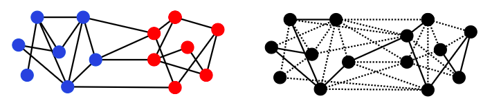
Two vertices are connected by an edge with probability if , if , and if . Self-loops do not occur. Each edge status is revealed independently with probability for a constant . The output is a graph with edge statuses given by . We denote this censored model by . In the symmetric case where , we denote the model by . For a visualization of the model, see Figure 1.
Objective. We observe a graph from with vertex labels removed (i.e., is unknown), and edges labeled by . An estimator is said to achieve exact recovery if
{eq}
lim_n→∞(∃s∈{±1}: ^σ= sσ_0) = 1.
We say that exact recovery is possible if there exists some estimator such that (2.1) holds.
Next, we provide formal statements of the main results, along with the key conceptual contributions.
2.2 Optimality of the spectral algorithm in the symmetric case.
Consider the symmetric case and . Throughout, we assume that and are fixed. We will establish that the information-theoretic threshold for exact recovery is given by: {eq} t_c(p,q):= 2(p- q)2+ (1-q- 1-p)2. Our first result shows that if , then any estimator fails to achieve exact recovery with high probability.
Theorem 2.1
If , then any estimator satisfies .
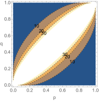
Figure 2 illustrates the region . Next, we describe the success of a simple spectral algorithm for . To this end, we need a weighted version of the signed adjacency matrix. Let {eq} y = y(p,q) = log(1-q1-p)log(pq), and define the signed adjacency matrix as
Note that whenever . Our next result shows that the spectral algorithm achieves exact recovery for .
Theorem 2.2
Let be the top eigenvector of and define . If and , then there exists and such that, with probability ,
Consequently, achieves exact recovery for . If , all conclusions hold if we replace by .
The estimator does not require additional clean-up steps. For the non-censored SBM, Abbe et. al. [Abbe2020] established an analogous result using entrywise eigenvector perturbation analysis, which we will also use (see Proposition 5.1). The key distinction of our algorithm to that of Abbe. et. al. [Abbe2020] lies in the fact that the observed graph admits a ternary encoding as opposed to a binary encoding. It is worthwhile to remark that the choice of is important for the spectral algorithm to succeed up to the information theoretic threshold, and in fact, (2.2) is the only choice of that works. Intuitively, is the ratio of evidence provided by a present edge on a vertex’s community as compared to an absent edge. More precisely, if we compute the log-likelihood ratio for a vertex to be in one community or the other, then it turns out to be a linear function of the number of present and absent edges to each community. In the symmetric case, the ratio of the coefficients corresponding to present and absent edges to Community turns out to be for both . When , i.e., in the special case considered in [ABBS14, Hajek2016], we have that , and the relative information provided by present and absent edges are equal. Therefore, Theorem 2.2 shows that the spectral algorithm with would succeed in exact recovery in the model of [ABBS14, Hajek2016].
We conclude this section by showing that the error rate of the spectral algorithm is close to that of the best possible estimator. For an estimator , we define the error rate as {eq} Err(^σ) = [min_s∈{-1,+1} 1n ∑_i=1^n 1_{^σ(i) ≠s σ_0(i)} ]. To define the best estimator, we use a genie-aided approach. Suppose that we want to find the label of . Now, in addition to the observed edge-labeled graph , suppose a genie gives us . The genie-based estimator minimizes the probability of making an error given these observations. More precisely, the genie-based estimator is given by {eq} ^σ_Best(u)&:=argmax_r∈{±1} (σ_0(u) = r ∣G, (σ_0(v))_v∈[n]∖{u}). The next result shows that the error rate of is within a factor of the error rate of :
Theorem 2.3
For any fixed , the spectral and genie-aided estimators satisfy
Therefore, the expected number of misclassified vertex-labels by the spectral algorithm is at most times that of the genie estimator. In particular, if , then this expected number is which is why exact recovery is achievable by the spectral algorithm.
Remark 2.1
If are unknown, then it is not difficult to estimate them. Indeed, if respectively denote the number of edges and triangles in the graph then and with probability tending to 1. We can use these to find consistent estimator of and use the spectral algorithm with . The conclusions of Theorem 2.2 and Theorem 2.3 still remain valid.
2.3 Beating the spectral algorithm
Theorems 2.2 and 2.3 strongly support the success of the spectral algorithm. We next provide results to show that there is room for improvement. First, Theorem 2.3 proves a relative discrepancy between the error rates of the spectral and the genie estimators, and therefore, the expected difference between misclassified vertices under these two algorithms may grow with . We prove that with an additional clean-up step, one can in fact get a relative discrepancy between the error rates. Second, we consider the case where the connection probabilities within Community 1 () and Community 2 () differ. In this case, we show that the spectral algorithm does not always work up to the information-theoretic threshold. Intuitively, if , then the relative information provided by present and absent edges are different for vertices in different communities. For this reason, it is not possible to find a common choice of encoding which works well for vertices in both communities. We establish the failure of the spectral algorithm rigorously for and . On the other hand, an algorithm based on degrees and an additional clean-up step turns out to be near-optimal for any .
We start by introducing the two-step estimator for which we need some notation. For a given vertex and , let be the degree profile where (resp. ) are the number of present and absent edges to vertices in Community 1 (resp. Community 2). Note that depends only on and . Define by {eq} Γ(u,σ, p_1,p_2,q) &= D_1(σ,u) logp1q + D_2(σ,u) log1-p11-q + D_3(σ,u) logqp2 + D_4(σ,u) log1-q1-p2
Definition 2.2 (Two-step estimator)
Given an initial estimator , a two-step estimator is computed as follows: {eq} ^X(^σ,u) = {+1 if Γ(u,^σ, p1,p2,q) ≥0,-1 otherwise.
The function is designed to mimic the workings of the genie estimator. In fact, we will later show that if and only if (see Proposition 6.1). Thus the two-step estimator treats the initial estimator as a proxy of the true community assignment and then does the same procedure as the genie estimator. The following result states that the two-step version of the spectral estimator has a sharper error rate in the symmetric case.
Theorem 2.4
If and , then for any ,
Next, we show that, for , the two-step estimator based on degrees in the observed graph has similar strong recovery guarantees. Let be the number of present edges incident to vertex . Define the degree-based estimator to be
Let , and and define {eq} t_c(p_1,p_2,q) = [1 - 12 min_x ∈[0,1] ∑_i(c_1)_i^x(c_2)_i^1-x ]^-1. When , then it is elementary to check that the minimum in (2.3) is attained for and therefore {eq} t_c(p,p,q) = t_c(p,q), where is given by (2.2). We next provide success guarantees for .
Theorem 2.5
If are distinct, then for any ,
Furthermore, if , then achieves exact recovery.
Remark 2.2
If , , and are unknown, then one can estimate them as follows. First, classify each vertex according to whether its degree is above average. This procedure will result in an estimator with at most errors on average, i.e., for some . Then we can estimate the parameters by counting revealed edges and non-edges between and within the estimated communities.
If , then cannot achieve spectral recovery. In this sense, Theorem 2.4 and Theorem 2.5 are complementary. We next describe the failure of the spectral algorithm for and . Let us start by defining a version of the spectral algorithm which makes decisions based on arbitrary linear combinations of the top two eigenvectors of some encoding matrix.
Definition 2.3
Given an encoding parameter , threshold and constants , let be the signed adjacency matrix with entries . Let and be the two top eigenvectors of . Then the spectral algorithm outputs the estimator {eq} ^σ(i) = sign(γ_1(u_1)_i + γ_2 (u_2)_i -r).
In other words, the spectral algorithm decides community assignments using a thresholding on a linear combination of the top two eigenvectors of some encoding matrix. Only the top two eigenvectors are included since the eigenvectors of behave like noisy versions of the eigenvectors of the rank- matrix . The following result states that even this more general algorithm fails in the antisymmetric CSBM for sufficiently close to the recovery threshold.
Theorem 2.6
Let and . There exists such that if , then, for any choice of , the algorithm fails to achieve exact recovery with probability .

Theorems 2.5 and 2.6 together show that there is a range of values of where the spectral algorithm fails in exact recovery, but succeeds (see Figure 3). In other words, there is a strong separation between the spectral algorithm and the two-step procedure based on degrees. One can now see the failure of the spectral algorithm from a technical perspective. In this regime, the top two eigenvectors of the encoding matrix are close to and respectively where is the -th largest eigenvector of the expectation matrix. If we imagine replacing and in (2.3) by their approximations, then the decision rule for the label of a vertex is given by the sign of for some coefficients and threshold , where denotes the degree profile of . Moreover, due to the choice of the encoding, the coefficients satisfy . The estimator that minimizes the error probability can also be shown to decide communities based on the sign of , but in order to satisfy the additional condition , one requires , or . For this reason, the spectral algorithm is strictly less powerful than the best possible estimator and thus one cannot expect the spectral algorithm to work all the way up to the information theoretic threshold if . Theorem 2.6 makes this intuition precise for .
Organization. The remainder of the paper is structured as follows. We start by setting up some preliminary notation in Section 3. In Section 4, we prove impossibility for the exact recovery problem in Theorem 2.1. Section 5 is devoted to entrywise perturbation analysis of the largest eigenvector of and completing the proof of Theorem 2.2. The error analysis for the spectral algorithm and the genie estimator will be provided in Section 6 and hence the proof of Theorem 2.3 will be completed. In Section LABEL:sec:two-step, we analyze the two-step estimator for a general class of initial estimators. This allows us to complete proofs of Theorems 2.4 and 2.5. Finally, we conclude with a proof of Theorem 2.6 regarding failure of the spectral algorithm in Section LABEL:sec:failure. We provide proof ideas at the beginnings of Sections 4-LABEL:sec:failure.
3 Notation and preliminaries
Let . We often use the Bachmann–Landau notation etc. For two sequences and , we write as a shorthand for . We write if and are asymptotically equivalent, namely for some . Additionally, we write if these sequences differ by a polylogarithmic factor asymptotically, namely there exists some constant such that and . For random variables , we write as a shorthand for in probability.
For a vector , we define and . For a matrix , we use to refer to its -th row, represented as a row vector. Given a matrix , is the spectral norm, and is the matrix norm. We use the convention that denotes natural logarithm, and write to mean . Finally, refers to the Kullback–Leibler divergence of two Bernoulli random variables with parameters and :
Let and . Note that since are marginally distributed as , we have that for all ,
| (3.1) |
with probability at least . We will often use (3.1) with . Additionally, let be the number of vertices whose connections to are revealed: . By [JLR00, Corollary 2.4] for
| (3.2) |
for all sufficiently large . We will use (3.2) with or .
The following Poisson approximation will be used throughout.
Lemma 3.1
Let be i.i.d. from a distribution taking three values and , , and . Let for . If , and , then
where is the probability that a random variable takes value .
The proof follows using Stirling’s approximation; we provide the details in Appendix LABEL:sec:appendix-2.
4 Impossibility of exact recovery
In this section, we give the proof of Theorem 2.1. We first identify a sufficient condition under which any algorithm fails to achieve exact recovery (Proposition 4.1). The condition captures the idea that there are some graph instances that cannot be labeled correctly with confidence since there are multiple suitable labelings for these instances. If these graph instances are likely to occur, then the overall failure probability can be lower-bounded. Theorem 2.1 is then proven by finding a set of graphs that are difficult to label correctly.
4.1 Sufficient condition for impossibility.
Recall that is the space of possible values of . We write as a generic notation to denote the observed value of the edge-labeled graph consisting of present, absent and censored edges. Also, let be the space of all possible values of . We write to denote the probability distribution of when the community assignments are given by .
Since
the estimator that maximizes the posterior probability for all also minimizes the error probability . This estimator is the Maximum A Posteriori (MAP) estimator. Thus, an optimal algorithm is devised by choosing uniformly at random among all MAP estimates, and we denote the corresponding estimator by . Next, using the fact that is uniformly distributed on , we must have . Then,
| (4.1) |
i.e., the MAP estimator coincides with the Maximum Likelihood estimator.
In light of this equivalence, the following result identifies a condition where the MAP estimator fails with a given probability.
Proposition 4.1
Fix . Suppose that there is with such that the following holds for any : There are pairs of vertices with opposite community label such that if is obtained by swapping any one of the labels of and , then . Then, conditionally on , the MAP estimator fails in exact recovery with probability at least .
-
Proof.
By our underlying condition, whenever , the true assignment is such that swapping one of the community assignment of one of the pairs among results in an equiprobable assignment. In that case, the algorithm is incorrect with probability at least , due to (4.1). Therefore, {eq} (^σ_MAP≠σ_0 | σ_0) ≥(^σ_MAP≠σ_0 | G ∈G’, σ_0) (G ∈G’ | σ_0) ≥δ(1- 1k), and the proof follows.
Remark 4.1
Additionally, Proposition 4.1 holds when is an assignment with equal community sizes, i.e., . In this case, observe that we can treat the assignment as though it were chosen uniformly at random from all satisfying . To see this, consider applying a uniformly chosen random permutation to the vertices. The inference problem does not change; however, the MAP estimator again coincides with the Maximum Likelihood estimator, and one can use an identical argument as above.
4.2 Proof of impossibility of exact recovery
-
Proof.
(Proof of Theorem 2.1). Throughout the proof, we condition on such that , which occurs with probability at least by (3.1). For convenience, we write instead of . We will show that with high probability, there exist pairs of vertices with opposite communities such that swapping their labels results in an equiprobable graph instance. By Proposition 4.1, this would show that exact recovery fails with probability for any algorithm.
For , let be sets of randomly selected vertices from Community 1 and Community 2, respectively. Let . Next, let be the set of all vertices in whose connections to all other vertices in are censored. We claim that with probability . To see this, observe that the expected number of revealed connections between vertices in is at most , so with high probability there are fewer than such connections. Therefore with high probability there are fewer than vertices with at least one neighbor in , from which the claim follows.
Now, let , , and . Let be the probability that a vertex in Community 1 has exactly present edges and absent edges to vertices in each community, conditioned on . By Lemma 3.1, we have
This implies that because since . Repeating the calculation for the case that is in Community 2, we conclude that the probability that a given vertex has exactly present edges and absent edges to vertices in each community is .
For , let be the indicator that has exactly present edges and absent edges to each community. Note that the random variables in the set are mutually independent conditionally on . Finally, observe that if and satisfy , then switching the community labels of and results in an equiprobable outcome.
Let
It suffices to show that there is a function such that with probability . We prove the claim for , and the proof for follows similary. Observe that conditioning on ,
Fix . By Chebyshev’s inequality,
Recall that with probability . Therefore, using , we have with probability . We conclude that
Recalling that , we have shown that there is a function such that . Similarly, using , it holds that . Applying Proposition 4.1 with and completes the proof.
Remark 4.2
We could generalize this to an argument that recovery is impossible whenever by arguing that there will be vertices with degree profiles of
in both communities, where takes on the value used in the computation of . The argument that this holds is largely analogous to that in the proof above, although one needs to use the fact that the criterion used to choose implies that vertices in each community are approximately equally likely to have this community profile and then bound both probabilities by bounding the weighted geometric means of their obvious formulations with weights and .
5 Analysis of the spectral algorithm
Recall the signed adjacency matrix from Section 2.2. The key to establishing Theorem 2.2 is the method of entrywise eigenvector analysis of [Abbe2020]. Let us denote , and let denote the -th eigenvector-eigenvalue pair of , where are arranged in non-decreasing order. Abbe et. al. [Abbe2020] show that, under a set of general conditions, in the -norm. Results of this kind were also derived recently by Lei [Lei2019]. Thus, if we can show that the signs of recover the communities with high probability (up to a global flip), and the magnitude of its entries are bounded away from zero, then the signs of also recover the communities with high probability. More precisely, using the methods of [Abbe2020, Theorem 2.1], we will establish the following result:
Proposition 5.1
With probability we have
for , where is a constant depending only on , , and .
In Section 5.1, we will provide a main result of [Abbe2020], specialized to our setting. In Section 5.2, we prove Proposition 5.1. With this result in hand, we provide the proof of Theorem 2.2 in Section 5.3.
5.1 Prior work on entrywise eigenvector analysis.
We start by reproducing [Abbe2020, Theorem 2.1], specialized to the case where is a rank-2 matrix and we wish to approximate a single eigenvector.
Theorem 5.1
([Abbe2020, Theorem 2.1]). Let be a symmetric random matrix and . Suppose that the following conditions hold with some and :
-
(i)
(Incoherence) , where and .
-
(ii)
(Row- and column-wise independence) For any , the entries in the -th row and column of are independent with others.
-
(iii)
(Row concentration) Suppose is continuous and non-decreasing in with , is non-increasing in , and . For any and ,
-
(iv)
(Spectral norm concentration) Let . Suppose and for some ,
Then with probability at least ,
for , where hides an absolute constant.
Next, we state the following two lemmas to verify the final two conditions in Theorem 5.1. The first is similar to [Hajek2016, Theorem 9].
Lemma 5.1
There exists such that
The following lemma is similar to [Abbe2020, Lemma 7].
Lemma 5.2
Let be a fixed vector, be independent random variables where , , and . Let . Then
The proofs of the above lemmas will be provided in Appendix LABEL:sec:appendix-supporting.
5.2 Proof of eigenvector approximation result.
We start by determining the eigenvalues and eigenvectors of .
Lemma 5.3
If , then has rank 2. If , then with probability at least , the eigenvalues of are given by
and the corresponding eigenvectors and are respectively given by if , if , and the other eigenvector has for all .
-
Proof.
Recall the edges are revealed independently with probability . Thus, for such that ,
(5.1) and similarly, for ,
(5.2) If , it follows that
By (3.1) with e.g. , we have that with probability at least . We now consider what happens to the eigenvalues of when are perturbed.
More generally, let denote an block matrix with blocks of size and , where the diagonal blocks take value and the off-diagonal blocks take value . Let be an eigenvalue of and let be the corresponding eigenvalue of . Let . By Weyl’s inequality,
In particular, if , , and , then . We conclude that when , the eigenvalues of are the same as the even communities case up to a factor.
Regarding the eigenvector , its entries are given by depending on community membership, in the case of . When , then determining the entries of the eigenvector requires solving a system of the form
Since and , the coefficients of the system are perturbed by a factor relative to the equal-sized communities case. Therefore, the eigenvector entries are also perturbed within a factor.
-
Proof.
(Proof of Proposition 5.1). We will apply Theorem 5.1 by verifying its conditions. In this proof, we avoid writing the terms for in Lemma 5.3 since that does not affect the asymptotic computations. We give the proof first for the case . By Lemma 5.3, it follows that
Let
where is the value from Lemma 5.1. Let
To check Condition i, recall that . Thus, by (5.1) and (5.2),
On the other hand, . Condition i therefore holds for large enough. Condition ii holds since the entries are independent conditioned on the communities. The first requirement of Condition iv is satisfied for sufficiently large since as , and . The second requirement is satisfied by Lemma 5.1, with . Finally, to verify Condition iii, fix , and apply Lemma 5.2 with , and setting . Note that equals or depending on whether or not, and let which equals to either or . Thus, . Then
Observing
Condition iii holds with . Applying Theorem 5.1, with probability at least ,
where depends only on , , and .
In the case , we replace by . Replacing all instances of by , the proof follows verbatim.
5.3 Success of the spectral algorithm.
We will use the following concentration result which can be proved analogously to the Chernoff bound. The proof of this lemma is provided in Appendix LABEL:sec:appendix-supporting.
Lemma 5.4
Let be constants such that and . Suppose . Let be i.i.d. where , , and and is given by (2.2). Let be i.i.d. where , , and , independent of the ’s. For any , we have the following:
-
Proof.
(Proof of Theorem 2.2). Consider the case . Let
Note that , and indeed is much smaller. Therefore, it is sufficient to analyze events conditioned on .
For any labeling , define . Let be such that is minimized. Then, by Proposition 5.1, with probability , {eq} n min_i ∈[n] s σ_0(i) (u_1)_i ≥n min_i ∈[n] σ_0(i) (A u1⋆)iλ1⋆ - C (loglogn )^-1, where we have used . We now show that is bounded away from zero. By Lemma 5.3, takes values or depending on , conditioned on . Thus, for each ,
Observe that for , {eq} &P(n σ_0(i)(A u1⋆)iλ1⋆ ≤2 εlog(pq)t (DKL(p∥q) + DKL(q∥p) ) | C_n )
= P(∑_j ∈J_i(σ_0) A_ij - ∑_j ∉J_i(σ_0) A_ij ≤εlog(n) | C_n ). By Lemma 5.4, if we have with given by (2.2), then there exists so thatBy a union bound and using (5.3), we conclude that there exists such that with probability , {eq} n min_i ∈[n] s σ_0(i) (u_1)_i ≥η.
In the case , we replace by , and the proof follows verbatim.
Remark 5.1
6 Asymptotic error of the genie estimator
In this section, we complete the proof of Theorem 2.3. In order to analyze the genie estimator, we first use the fact that the prior on is uniform, so that
In other words, the genie estimator may be interpreted as a Maximum Likelihood Estimator. Recall from (2.3) and the notation for the degree profile from Section 2.3. We first derive an expression for the genie estimator for general CSBM with possibly arbitrary choices of . This result will also be useful in the next section.
Proposition 6.1
For any , we have for all {eq} ^σ_Best(u) = {+1 if Γ(u,σ0, p1,p2,q) ≥0-1 otherwise.
The proof is provided in Appendix LABEL:appendix-3. In other words, the genie estimator decides community assignments based on the sign of a linear combination of the degree profiles. For , it is not difficult to see that if is given by (2.2), then we get the following cleaner expression in terms of the signed adjacency matrix: {eq} Γ(u,σ, p,p,q) &= (∑_v∈J_u(σ) A_ij - ∑_v∉J_u(σ)A_ij)logpq, where . Thus, we see that in the symmetric case, the genie estimator decides the communities based on the sign of . From the proof of Theorem 2.2, we see that the spectral algorithm recovers successfully if when and when where (see (5.3)). Thus it intuitively makes sense that the error rates of and should be close.
We proceed with an error analysis of the genie-based estimator in Section 6.1, which will be used to complete the proof of Theorem 2.3 in Section LABEL:sec:genie-result-theorem
6.1 Error analysis of the genie-based estimator.
Next we analyze the error rate of the genie-based estimator . Recall the error rate from (2.2) and from (2.3).
Lemma 6.1
.
-
Proof.
Let . Then . Note that, since almost surely, we have
Therefore,
It suffices to show that and .
Computing . Fix and let us compute . Estimating is a binary Bayesian hypothesis testing problem, where the prior is given by . We are given the observed edge-labeled graph and , which satisfies (3.1) with with probability at least . The genie-based estimator performs a Maximum A Posteriori (MAP) decoding rule based on the observed degree profiles . Let . By (3.2),
Using Lemma 3.1,
We can now use [AS15, Theorem 3] with , and to conclude that {eq} (^σ_Best(u) ≠σ_0(u)) & = n^-Δ_t(c_1’,c_2’) (1+o(1)) + n^-ω(1), where {eq} Δ_t(c_1’,c_2’) : = max_x∈[0,1] ∑_i (x(c’_1)_i +(1-x)(c’_2)_i -(c’