A Diffuse Interface Model for Cell Blebbing Including Membrane-Cortex Coupling with Linker Dynamics

Abstract

The aim of this paper is to develop suitable models for the phenomenon of cell blebbing, which allow for computational predictions of mechanical effects including the crucial interaction of the cell membrane and the actin cortex. For this sake we resort to a two phase-field model that uses diffuse descriptions of both the membrane and the cortex, which in particular allows for a suitable description of the interaction via linker protein densities.

Besides the detailed modelling we discuss some energetic aspects of the models and present a numerical scheme, which allows to carry out several computational studies. In those we demonstrate that several effects found in experiments can be reproduced, in particular bleb formation by cortex rupture, which was not possible by previous models without the linker dynamics.

68Q25, 68R10, 68U05

1 Introduction

The formation of special membrane protrusions in eukaryotic cells has drawn the attention of biologists for a couple of decades now (cf. [9, 11]), and is also referred to as “cell blebbing”.

Figure 1: A simple cell scheme.

Cell blebbing has been observed during apoptosis [21], cytokinesis, and mitosis [6, 27], but also as a means for locomotion [37] in primordial germ cells or cancer cells. In order for a cell to move in a certain direction via blebbing, the site of bleb nucleation towards that direction has to be specified. It has not yet been fully understood what triggers the formation of a bleb at a specific cell site. However, theories about relevant influences exist and a mathematical model for studying the mechanisms that lead to bleb site selection has been recently proposed in [12]. In this work, we do not deal with this phase in the process of cell blebbing: our model targets the process after bleb site selection and is aimed at investigating the mechanics of bleb formation. Previous works on this topic are, e.g., [23, 36, 35, 5, 4, 34, 40]. Lim et al. [23] present a one-dimensional model focusing on bending and surface energy of the membrane and include another important energy for the influence of so-called linker proteins (see below) that also play a role in the development of membrane protrusions. The authors of [36, 35] deal with the interaction between membrane components and the surrounding fluid. In [5, 4] one-dimensional models which concentrate on the dynamics of the linker protein density are investigated. Stinner et al. [34] propose a finite element method (FEM) for simulation of bleb heights on two-dimensional surfaces incorporating bending energy and linker effects as well.

The aim of this paper is to propose a fully integrated three-dimensional model that takes forces of the surrounding fluid, linker protein effects as well as bending and surface energies into account. In the following, we will treat bleb formation as a fluid-structure interaction problem with two diffuse interfaces, the membrane and the cortex (see below), which are immersed in a fluid. On the cortex, we model the linker proteins with a density function and include their forces on the membrane thus introducing a coupling between cortex and membrane. We will show how this coupling can be incorporated in a potential energy functional that also comprises surface and bending energy of the membrane and cortex. By leveraging Onsager’s variational pinciple, we will arrive at a system of partial differential equations (PDEs) with evolution laws for the diffuse interfaces as well as a Navier-Stokes system for the fluid flow. Additionally, we will have a reaction-diffusion-type PDE for the linker proteins concentrated on the cortex.

1.1 Notation

We denote the $n$-dimensional Lebesgue measure by $\mathfrak{L}^{n}$ and the Hausdorff measure of Hausdorff dimension $m$ by $\mathfrak{H}^{m}$. The normal of a surface $\mathcal{S}$ is ${\nu}_{\mathcal{S}}$. The surface material derivative is $\partial^{\circ}\rho$ and the surface gradient on a surface $\mathcal{S}$ is denoted by $\nabla_{\mathcal{S}}\rho$. The gradient for a Gateaux derivative of $f$ in space $X$ is denoted $\nabla^{X}f$. $\mathbb{P}_{k}$ denotes a simplicial element with polynomials of degree at most $k~{}$. Sobolev spaces of $k$-times weakly differentiable, $L^{2}$ functions is $H^{k}\left(\Omega\right)$. The space of solenoidal functions is denoted $H^{1}_{\sigma,0}\left(\Omega\right)$.

2 Modeling

In the following we discuss the modelling of cell blebbing using diffuse interfaces. We start with a brief overview of the process before proceeding to a more mathematical level:

2.1 Biological Background

Let us briefly clarify some basic parts of a cell and the principle processes taking place when blebbing occurs.

Fig. 1 shows a simple cell scheme that hints to the following components of a cell:

• The cell membrane (solid black circle) is a bilayer of lipid molecules and encloses the whole cell.

• The cell cortex (dotted black circle) is a network of actin fibres, which are elastic and can be contracted by myosin motors (green ellipses).

• The cytosol is a fluidic material that fills up the whole cell and contains various different objects, which we do not model here explicitly, but within the fluid viscosity.

• Linker proteins (orange small circles) connect the cell membrane and cell cortex. They are also elastic to a certain extent until they are overstretched and in turn ripped apart. We model them as Hookean springs.

The cell is surrounded by a region called the extracellular matrix, which is also filled with a fluid. In our model, we assume for simplicity a mixture of the cytosol and the fluid in the extracellular matrix.

The phenomenon of cell blebbing may be outlined as follows (cf. description in [11]): Initially, the cell cortex may be contracted by the myosin motors as a result of chemical reactions, or the cortex may be destroyed by external influence. In turn, cytosol flows towards the cell membrane (being either pushed by the cortex or pressed through a hole in case of a destroyed cortex), which is then elongated forming a protrusion that is called a bleb. This development is hindered by influences like surface tension and flexural rigidity of the cell membrane, as well as the linker proteins, which pin the cell membrane to the cell cortex. However, if the pressure resulting from the cell cortex contraction surpasses a critical value, the linker proteins break and the speed of bleb development changes qualitatively (cf. [23, p. 3], [40, p. 44]); this is called bleb nucleation. Subsequently, the phase of bleb retraction starts by reformation of the cortex. Furthermore, broken linker proteins are rebuilt and reconnect to the membrane. In the end, the proteins pull the membrane towards the cortex and the bleb vanishes. This process is called ‘bleb retraction’ or ‘bleb healing’.

2.2 Phase Field Model

The cell with all its components is contained in a compact set $\Omega\subseteq\mathbb{R}^{3}$. Our model comprises two diffuse layers, the cell membrane and cortex, both with width of order $\varepsilon>0$. They are represented by the phase field functions ${\phi},{\psi}\colon\Omega\rightarrow\mathbb{R}$ that are supposed to approach the value $-1$ on the regions enclosed by the cell membrane and cell cortex, respectively, and $1$ on the corresponding outer regions. In between these regions, the functions ${\phi}$, ${\psi}$ interpolate smoothly and cross zero where the diffuse layers are to be expected. Phase field methods have been successfully applied in materials science [33] and for two-phase fluid flow [1], where they have been motivated by thermodynamic theories of phase separation.

The membranes surrounding eukaryotic cells are typically bilayers of lipid molecules. Assuming the fluid to be lipophobic, say we are dealing with water, we expect the cell membrane to show phase separation behaviour like, e.g., oil in water. For simplicity, we assume the same behaviour for the cell cortex, although the interaction of actin with water is more complex.

The Canham–Helfrich Energy

Canham [7] and Helfrich [19] both suggested a model for the energy associated to biomembranes. They basically came up with the following expression for a membrane $\mathcal{M}$ as two-dimensional surface:

$$\int_{\mathcal{M}}\frac{\beta}{2}\left({H}\left(x\right)-{H}_{0}\right)^{2}+\gamma\;\mathrm{d}\mathfrak{H}^{2}(x)+\kappa_{G}\int_{\mathcal{M}}{K}\left(x\right)\;\mathrm{d}\mathfrak{H}^{2}(x),$$

where $\beta$ is the flexural rigidity, ${H}_{0}$ is the spontaneous mean curvature (the mean curvature the membrane tends to in unconstrained situations), $\gamma$ is the surface tension, and $\kappa_{G}$ is the Gaussian flexural rigidity of the membrane. The spontaneous curvature may be employed to reflect asymmetries in the membrane, e.g., due to chemical influence (cf. [32, Sec. 2.5.2]). The Gaussian curvature is constant across a set of surfaces with the same topologial genus. Hence, since we do not consider topological changes, we may as well neglect the Gaussian bending term when varying the energy functional.

In order to employ the Canham–Helfrich energy in our phase field model, we need diffuse counterparts of the surface $\int_{\mathcal{M}}\gamma\;\mathrm{d}\mathfrak{H}^{2}$ and bending $\frac{\beta}{2}\int_{\mathcal{M}}\left({H}\left(x\right)-{H}_{0}\right)^{2}\;\mathrm{d}\mathfrak{H}^{2}(x)$ energies. It is well-known that the Ginzburg-Landau energy

$${\mathcal{G}}\left[\phi\right]{}=\gamma\int_{\Omega}\frac{\varepsilon}{2}\left\lvert\nabla\phi\right\rvert^{2}+\frac{1}{\varepsilon}{W}\left(\phi\right)\;\mathrm{d}\mathfrak{L}^{3}=\gamma\int_{\Omega}{g}_{\varepsilon}\left[\phi\right]\;\mathrm{d}\mathfrak{L}^{3}$$

$\Gamma$-converges to the former as $\varepsilon\downarrow 0$ (up to a constant factor, cf. [25, 24]). Moreover, it has been proven in [29] (and independently in [26] for two dimensions) that the functional

$${\mathcal{W}_{0}}\left[\phi\right]=\frac{1}{2\varepsilon}\int_{\Omega}\left(-\varepsilon\Delta\phi+\frac{1}{\varepsilon}W^{\prime}\left(\phi\right)\right)^{2}\;\mathrm{d}\mathfrak{L}^{3}$$

$\Gamma$-converges to the Willmore functional. In [13], this functional has been extended to the more general case of spontaneous mean curvature such as

$${\mathcal{W}_{C_{0}}}\left[\phi\right]=\frac{1}{2\varepsilon}\int_{\Omega}\left(-\varepsilon\Delta\phi+\left(\frac{1}{\varepsilon}\phi+C_{0}\right)\left(\phi^{2}-1\right)\right)^{2}\;\mathrm{d}\mathfrak{L}^{3}.$$

So the “diffuse” Canham–Helfrich energy we employ in the following is given by

$${\mathcal{CH}}\left[\phi\right]={\mathcal{W}_{C_{0}}}\left[\phi\right]+{\mathcal{G}}\left[\phi\right]{}$$

for the membrane phase field and analogously for the cortex phase field.

2.3 Mechanics of the Bulk

The bulk region $\Omega$ is assumed to be filled completely by a fluid. The movement of the fluid body in the course of time shall be described by a sufficiently smooth invertible map ${X}$. At the boundary $\partial\Omega$ of $\Omega$, we prescribe that the wall is impenetrable by the fluid

$$\partial_{t}{X}\left(\cdot,x\right)\cdot{\nu}=0,\quad\forall x\in\partial\Omega,$$

as well as no slip conditions

$$\partial_{t}{X}\left(\cdot,x\right)\cdot\tau=0,\quad\forall x\in\partial\Omega,$$

where $\tau$ is any tangential vector of $\partial\Omega$. A fluid particle can be specified by its initial position (at $t=0$) $\bar{x}\in\Omega$, also called its label or Lagrangian coordinate, and its current position, or Eulerian coordinate, $x={X}\left(t,\bar{x}\right)$. The Lagrangian velocity is given by $\mathcal{V}(t,\bar{x})=\partial_{t}{X}\left(t,\bar{x}\right)$, and thus its Eulerian counterpart is ${v}\left(t,x\right)=\mathcal{V}(t,X^{-1}\left(t,x\right))$. In this regard, we introduced two interpretation frames in which the velocity of a deformation may be studied: In the Lagrangian frame $\mathcal{V}(t,x)$ assigns to a particle $x\in\Omega$ its velocity at a given time. In the Eulerian frame, $x$ is no longer a particle identifier, but a point in space to which the velocity ${v}\left(t,x\right)$ of the particle passing through $x$ at time $t$ is assigned. In the following, we may switch between these two observer positions as suited.

All forces inside the Eulerian fluid body are defined by the Cauchy stress tensor

$${\mathbb{T}}={\sigma}-{p}I_{3},$$

which can be separated into a part accounting for stress due to particle friction, the viscous stress tensor ${\sigma}$, and a part that captures the elastic collisions of the fluid particles and is given by the hydrostatic pressure ${p}$.

The fluid considered in our model shall be isotropic and Newtonian. For the viscous stress tensor, we assume

$${\sigma}=\eta\left(\nabla{v}+{\nabla{v}}^{T}-\frac{2}{3}\nabla\cdot{v}I\right)+\zeta\nabla\cdot{v}$$

(cf. [20, Chapter II]), where $\eta$ and $\zeta$ are coefficients describing the viscosity of the fluid. This constitutive law prescribes a linearized version of the viscous stress tensor and is to be employed with care when large velocity gradients appear.

Furthermore, the fluid we consider throughout this work is incompressible, i.e.,

$$\nabla\cdot{v}=0.$$

A direct consequence is a simplification of the viscous stress tensor to

$${\sigma}=\eta\left(\nabla{v}+{\nabla{v}}^{T}\right).$$

2.4 Membrane-Cortex Coupling

As pointed out above, linker proteins pin the membrane to the cortex. In our model, we consider them as (macro-)molecules sticking to the cortex thus being transported with it. In this situation, it is not clear how to model the direction with which these molecules point out of the cortex and connect to the membrane. To mitigate this problem and leave a certain degree of freedom, we introduce a connectivity function ${\omega}$ such that ${\omega}\left(x,y,{\nu}_{\psi}\right)$ describes the probability with which a point $x\in\mathbb{R}^{3}$ on the cortex is connected to a point $y\in\mathbb{R}^{3}$ on the membrane in direction $y-x$. The function also depends on the normal approximation ${\nu}_{\psi}\left(x\right)=\frac{\nabla\psi(x)}{\left\lvert\nabla\psi(x)\right\rvert}$ for all points $x$ with $\nabla\psi(x)\neq 0$, which could be considered a gauge direction. For example, we may choose

(1) $${\omega}\left(x,y,{\nu}_{\psi}\right)=\tilde{\omega}\left(\frac{{\nu}_{\psi}\left(x\right)\cdot(y-x)}{\left\lvert y-x\right\rvert}\right)$$

and

(2) $$\tilde{\omega}\left(t\right)=\hat{\omega}\exp\left(\frac{\arccos(t)^{2}}{s^{2}}\right)$$

for some standard deviation $s$ and a scaling factor $\hat{\omega}$ to model Gaussian distribution of directions around the cortex normal.

In order to define the potential energy in the system due to this coupling, we use the Hookean spring model for the linker proteins: The energy assigned to a linker connecting $x$ and $y$ is

$$\frac{1}{2}\xi\left\lvert y-x\right\rvert^{2},$$

where $\xi$ is a spring constant. Let us assume the particle volume density of linkers connecting membrane and cortex at $p$ is given by the function ${\rho}_{a}\left(x\right)$. In case every linker at $x$ connects to $y$, the energy volume density at $x$ is then given by the expression

$${\rho}_{a}\left(x\right)\frac{1}{2}\xi\left\lvert y-x\right\rvert^{2}.$$

However, not every linker at $x$ might connect to $y$. This is exactly, where ${\omega}$ comes into play: In the more general scenario we consider here, the energy volume density at $x$ is given by

$$\int_{\Omega}{{\delta}}_{\varepsilon}\left[\phi\right](y){\omega}\left(x,y,{\nu}_{\psi}\right){\rho}_{a}\left(p\right)\frac{1}{2}\xi\left\lvert y-x\right\rvert^{2}\;\mathrm{d}\mathfrak{L}^{3}(y),$$

where the integral operator

$$u\mapsto\int_{\Omega}{{\delta}}_{\varepsilon}\left[\phi\right](y)u(y)\;\mathrm{d}\mathfrak{L}^{3}(y)$$

is meant to integrate a quantity $u$ over the membrane: Since we only have phase fields and no two-dimensional surfaces, we use a Dirac-like weight ${{\delta}}_{\varepsilon}\left[\phi\right]$ to concentrate the integral in the region of the diffuse membrane layer. We will describe below, how to choose ${{\delta}}_{\varepsilon}\left[\phi\right]$. Finally, the potential energy contained in the system due to this coupling can be measured by the double-integral

$${\mathcal{C}}\left[\phi,\psi,{\rho}_{a}\right]\colonequals\int_{\Omega}{{\delta}}_{\varepsilon}\left[\psi\right](x)\int_{\Omega}{{\delta}}_{\varepsilon}\left[\phi\right](y){\omega}\left(x,y,{\nu}_{\psi}\right){\rho}_{a}\left(x\right)\frac{1}{2}\xi\left\lvert y-x\right\rvert^{2}\;\mathrm{d}\mathfrak{L}^{3}(y)\;\mathrm{d}\mathfrak{L}^{3}(x).$$

2.5 Linker Protein Dynamics

Above we already used the density ${\rho}_{a}$ of proteins that connect membrane and cortex; we call them active. We already mentioned that the proteins are ripped apart when overstretched, but it has also been reported [11] that these broken entities may be repaired (or ‘healed’). As we aim at modeling the ripping and repairing processes, we introduce further a density ${\rho}_{i}$ of broken proteins that no longer connect, but may be repaired; these proteins are called inactive.

Both linker protein densities evolve due to three effects: The fluid transporting the cortex and the particles on it, surface diffusion, as well as ripping and repairing. If the cortex were a sharp interface, i.e., a surface, we would consider the reaction-diffusion system

$$\partial^{\circ}_{t}{}{\rho}_{a}-\nabla_{\Sigma}\cdot\left({\eta}_{a}\nabla{\rho}_{a}\right)+{\rho}_{a}\nabla_{\Sigma}\cdot{v} =k{\rho}_{i}-r\left[\Gamma\right]{\rho}_{a}\quad\quad \;\Sigma,$$ on

$$\partial^{\circ}_{t}{}{\rho}_{i}-\nabla_{\Sigma}\cdot\left({\eta_{i}}\nabla{\rho}_{i}\right)+{\rho}_{i}\nabla_{\Sigma}\cdot{v} =-k{\rho}_{i}+r\left[\Gamma\right]{\rho}_{a}\quad\quad \;\Sigma.$$ on

The parameters of this system are as follows: $k$ is a repairing rate, $r\left[\Gamma\right]$ a ripping rate that depends on the position of the membrane (if the membrane is far away from the cortex, the stretching of linkers is high; if the membrane is close, the stretching is low), and ${\eta}_{a},{\eta_{i}}\in\mathbb{R}$ are diffusivities. Note that the right hand sides have opposite signs, which ensures conservation of the number of particles on the surface.

Now let us extend the densities ${\rho}_{a}$, ${\rho}_{i}$ constantly in normal direction of $\Sigma$. We then can express

$$\partial^{\circ}_{t}{}\rho_{\alpha}=\partial_{t}\rho_{\alpha}+{v}\cdot\nabla\rho_{\alpha},\quad\quad\alpha\in\{a,i\}.$$

Decomposing ${v}={\mathrm{v}}{\nu}_{\Sigma}+v_{\tau}$ into a normal and tangential part, we find

$${v}\cdot\nabla\rho_{\alpha}=v_{\tau}\cdot\nabla\rho_{\alpha}$$

(the normal derivative of $\rho_{\alpha}$ is zero) and $\rho_{\alpha}\nabla_{\Sigma}\cdot{v}=-\rho_{\alpha}{H}{\mathrm{v}}+\rho_{\alpha}\nabla_{\Sigma}\cdot v_{\tau}$. Inserting into the above equations, we finally obtain

$$\partial_{t}{\rho}_{a}-{H}\mathrm{v}{}{}{\rho}_{a}-\nabla_{\Sigma}\cdot\left({\eta}_{a}\nabla{\rho}_{a}\right)+\nabla_{\Sigma}\cdot\left({\rho}_{a}v_{\tau}\right) =k{\rho}_{i}-r\left[\Gamma\right]{\rho}_{a}\quad\quad \;\Sigma,$$ on

$$\partial_{t}{\rho}_{i}-{H}\mathrm{v}{}{\rho}_{i}-\nabla_{\Sigma}\cdot\left({\eta_{i}}\nabla{\rho}_{i}\right)+\nabla_{\Sigma}\cdot\left({\rho}_{i}v_{\tau}\right) =-k{\rho}_{i}+r\left[\Gamma\right]{\rho}_{a}\quad\quad \;\Sigma.$$ on

Since we are not dealing with surfaces, but diffuse layers, we need to approximate the surface differential operators. As a first step, we reformulate the above equations in the sense of distributions employing a Dirac distribution $\delta_{\Sigma}$ concentrating mass on $\Sigma$, and an extension $\bar{{v}}$ of the velocity ${v}$ with ${\nu}_{\Sigma}\mathbin{\otimes}{\nu}_{\Sigma}\mathbin{:}\nabla\bar{v}=0$ such that $\nabla\cdot\bar{{v}}=\nabla_{\Sigma}\cdot{v}$. The reformulated equations contain only bulk differential operators:

$$\delta_{\Sigma}\partial_{t}{\rho}_{a}-\delta_{\Sigma}{H}\bar{\mathrm{v}{}{}}{\rho}_{a}-\nabla\cdot\left(\delta_{\Sigma}{\eta}_{a}\nabla{\rho}_{a}\right)+\nabla\cdot\left(\delta_{\Sigma}{\rho}_{a}\bar{{v}}_{\tau}\right) =\delta_{\Sigma}(k{\rho}_{i}-r\left[\phi\right]{\rho}_{a})\quad\quad \;\Sigma,$$ on

$$\delta_{\Sigma}\partial_{t}{\rho}_{i}-\delta_{\Sigma}{H}\bar{\mathrm{v}{}}{\rho}_{i}-\nabla\cdot\left(\delta_{\Sigma}{\eta_{i}}\nabla{\rho}_{i}\right)+\nabla\cdot\left(\delta_{\Sigma}{\rho}_{i}\bar{{v}}_{\tau}\right) =-\delta_{\Sigma}(k{\rho}_{i}+r\left[\phi\right]{\rho}_{a})\quad\quad \;\Sigma.$$ on

We then approximate $\delta_{\Sigma}$ by a smooth function ${{\delta}}_{\varepsilon}\left[{\psi}\right]$ that converges to $\delta_{\Sigma}$ for $\varepsilon\to 0$ in the sense of distributions. Also, we introduce phase field analogues for the mean curvature, the normal part of the velocity, and the corresponding tangential part, respectively:

$$\begin{split}{H}_{{\psi}}=\left\lvert\nabla{\psi}\right\rvert\left(-\varepsilon\Delta{\psi}+\varepsilon^{-1}W^{\prime}\left({\psi}\right)\right),\quad\quad\mathrm{v}_{{\nu}_{\phi}}{}=({v}\cdot{\nu}_{{\psi}}){\nu}_{{\psi}}+({v})_{\tau}.\end{split}$$

Thus, the following system in the bulk $\Omega$ is obtained:

(6a) $${{\delta}}_{\varepsilon}\left[{\psi}\right]\partial_{t}{\rho}_{a}-{{\delta}}_{\varepsilon}\left[{\psi}\right]{H}\mathrm{v}_{{\nu}_{\psi}}{}{\rho}_{a}-\nabla\cdot\left({{\delta}}_{\varepsilon}\left[{\psi}\right]{\eta}_{a}\nabla{\rho}_{a}\right)+\nabla\cdot\left({{\delta}}_{\varepsilon}\left[{\psi}\right]({v})_{\tau}{\rho}_{a}\right) ={{\delta}}_{\varepsilon}\left[{\psi}\right](k{\rho}_{i}-r\left[\phi\right]{\rho}_{a}),$$

(6b) $${{\delta}}_{\varepsilon}\left[{\psi}\right]\partial_{t}{\rho}_{i}-{{\delta}}_{\varepsilon}\left[{\psi}\right]{H}\mathrm{v}_{{\nu}_{\psi}}{}{\rho}_{i}-\nabla\cdot\left({{\delta}}_{\varepsilon}\left[{\psi}\right]{\eta_{i}}\nabla{\rho}_{i}\right)+\nabla\cdot\left({{\delta}}_{\varepsilon}\left[{\psi}\right]({v})_{\tau}{\rho}_{i}\right) ={{\delta}}_{\varepsilon}\left[{\psi}\right](-k{\rho}_{i}+r\left[\phi\right]{\rho}_{a}).$$

Now that the structure of the linker dynamics is fixed, it remains to specify the function $r\left[\phi\right]$ giving the ripping rate. Let us first discuss this function in the sharp interface setting. To obtain the ripping rate, we integrate over the membrane, where we weigh the area element by the connectivity and a ripping density $\tilde{r}$

$$r\left[\Gamma\right]=\int_{\Gamma}{\omega}\left(x,y,{\nu}_{\Sigma}\right)\tilde{r}(x,y)\;\mathrm{d}\mathfrak{H}^{2}(y).$$

The most common models for the ripping density are on the one hand a Kramer-type kinetic model derived in [15], and also employed by [5]:

(7) $$\tilde{r}(x,y)=k_{\text{off}}\exp\left(\frac{\xi{}\left\lvert y-x\right\rvert\delta}{Tk_{B}}\right).$$

On the other hand, [23] suggested a discontinuous approach towards modelling the linker forces: They take the linker force as the product of the Hookean force term and a step function:

$$\xi{}\left\lvert y-x\right\rvert\left(1-\frac{\left\lvert y-x\right\rvert}{\ell^{*}}\right)^{+}$$

with $(\cdot)^{+}$ denoting the non-negative part and $\ell^{*}$ a critical length above which the linkers rip. In this model, the linker ripping rate can be interpreted as being zero below the critical height and infinity above. Motivated by this approach, a ripping density of

$$\tilde{r}(x,y)=\frac{(\left\lvert y-x\right\rvert-\ell^{*})^{+}}{\vartheta}$$

for $\vartheta\ll 1$ has been used in [40] as a continuous interpolation. Going from sharp to diffuse, we only need to introduce a weight under the integral

$$\int_{\Gamma}{\omega}\left(x,y,{\nu}_{\Sigma}\right)\tilde{r}(x,y)\;\mathrm{d}\mathfrak{H}^{2}(y)\longrightarrow\int_{\Omega}{{\delta}}_{\varepsilon}\left[\phi\right]{\omega}\left(x,y,{\nu}_{\psi}\right)\tilde{r}(x,y)\;\mathrm{d}\mathfrak{L}^{3}(y).$$

3 A PDE Model via Onsager’s Principle

From these considerations, we can make an ansatz for a system of partial differential equations (PDEs) that should describe our physical system:

(8a) $$\rho(\partial_{t}{v}+\nabla{v}{v})-\nabla\cdot J_{{v}} =K,$$

(8b) $$\nabla\cdot{v} =0,$$

(8c) $$\partial_{t}{\phi}+{v}\cdot\nabla{\phi}-\nabla\cdot J_{{\phi}} =0,$$

(8d) $$\partial_{t}{\psi}+{v}\cdot\nabla{\psi}-\nabla\cdot J_{{\psi}} =0,$$

(8e) $${{\delta}}_{\varepsilon}\left[{\psi}\right]\partial_{t}{\rho}_{a}-\mathrm{v}_{{\nu}_{{\psi}}}{H}_{{\psi}}{\rho}_{a}-\nabla\cdot\left({{\delta}}_{\varepsilon}\left[{\psi}\right]{\eta}_{a}\nabla{\rho}_{a}\right)+\nabla\cdot\left({{\delta}}_{\varepsilon}\left[{\psi}\right]{\rho}_{a}({v})_{\tau}\right) =$$

$${{\delta}}_{\varepsilon}\left[{\psi}\right](k{\rho}_{i}-r\left[\phi\right]{\rho}_{a})$$ ,

(8f) $${{\delta}}_{\varepsilon}\left[{\psi}\right]\partial_{t}{\rho}_{i}-\mathrm{v}_{{\nu}_{{\psi}}}{H}_{{\psi}}{\rho}_{i}-\nabla\cdot\left({{\delta}}_{\varepsilon}\left[{\psi}\right]{\eta_{i}}\nabla{\rho}_{i}\right)+\nabla\cdot\left({{\delta}}_{\varepsilon}\left[{\psi}\right]{\rho}_{i}({v})_{\tau}\right) =$$

$${{\delta}}_{\varepsilon}\left[{\psi}\right](-k{\rho}_{i}+r\left[\phi\right]{\rho}_{a})$$ ,

(8g) $$\partial_{{\nu}}{\phi}|_{\partial\Omega}=\partial_{{\nu}}{\psi}|_{\partial\Omega} =0,$$

(8h) $$J_{{\phi}}|_{\partial\Omega}\cdot{\nu}=J_{{\psi}}|_{\partial\Omega}\cdot{\nu} =0,$$

(8i) $${\rho}_{a}|_{\partial\Omega} =0,$$

(8j) $${\rho}_{i}|_{\partial\Omega} =0,$$

and search for the thermodynamic fluxes $J_{{v}}$, $J_{{\phi}}$, $J_{{\psi}}$ and the force $K$. This is done by employing Onsager’s principle that postulates

(9) $$\min_{J_{{v}},J_{{\phi}},J_{{\psi}}}\left({\frac{\mathrm{d}}{\mathrm{d}\,t}}\left({U}\left[{v},\phi,\psi,{\rho}_{a}\right]\right)+{\Psi}\left(J_{{v}},J_{{\phi}},J_{{\psi}}\right)\right),$$

where the internal energy is given as the sum of the kinetic and free energy in the system:

$${U}\left[{v},\phi,\psi,{\rho}_{a}\right]=\frac{1}{2}\left\|{v}\right\|_{L^{2}\left(\Omega\right)}^{2}+{\mathcal{F}}\left[\phi,\psi,{\rho}_{a}\right],$$

and

$${\Psi}\left(J_{{v}},J_{{\phi}},J_{{\psi}}\right)=\int_{\Omega}\frac{\left\lvert J_{{v}}\right\rvert^{2}}{2\eta}+\frac{\left\lvert J_{{\phi}}\right\rvert^{2}}{2{m}\left({\phi}\right)}+\frac{\left\lvert J_{{\psi}}\right\rvert^{2}}{2m\left({\psi}\right)}\;\mathrm{d}\mathfrak{L}^{3}$$

is the functional that gives the dissipation in the system for the mobilities ${m}\left(\phi\right)$, $m\left(\psi\right)$.

We obviously need to calculate the time derivative of the internal energy. Before we will do so, we shall elaborate on the choice of the “diffuse Dirac functions” ${{\delta}}_{\varepsilon}\left[\phi\right]$ and ${{\delta}}_{\varepsilon}\left[\psi\right]$.

3.1 Phase Field Transport Formula

In the sharp interface setting, we encounter surface integrals $\int_{{X}\left(t,\Sigma\right)}f\;\mathrm{d}\mathfrak{L}^{3}$, for $f\colon\mathbb{R}\times\Omega\rightarrow\mathbb{R}$, whose time derivatives are treated by leveraging the classical surface transport formula (cf., e.g., [28])

$$\left.{\frac{\mathrm{d}}{\mathrm{d}\,t}}\left(\int_{{X}\left(t,\Sigma\right)}f\;\mathrm{d}\mathfrak{L}^{3}\right)\right|_{t^{*}}=\int_{{X}\left(t^{*},\Sigma\right)}\left.\partial^{\circ}_{t}\left(f\right)\right|_{t^{*}}+f\nabla_{{X}\left(t^{*},\Sigma\right)}\cdot\partial_{t}{X}\;\mathrm{d}\mathfrak{H}^{2}.$$

From the phase field perspective, surface integrals make no sense since there is no such two-dimensional structure. Nonetheless, the terms produced by application of the transport formula need to be represented in the phase field PDE system in order to achieve consistency with the corresponding sharp interface system for $\varepsilon\searrow 0$. Let us consider the bulk integral $\int_{{X}\left(t,\Omega\right)}f{{\delta}}_{\varepsilon}\left[{\phi}\right]\;\mathrm{d}\mathfrak{L}^{3}$ weighted by a characteristic for the diffuse layer analogue of $\Sigma$. The fluid deformation ${X}$ maps $\Omega$ onto itself, so

$${\frac{\mathrm{d}}{\mathrm{d}\,t}}\left(\int_{{X}\left(t,\Omega\right)}f{{\delta}}_{\varepsilon}\left[{\phi}\right]\;\mathrm{d}\mathfrak{L}^{3}\right)=\int_{\Omega}\partial_{t}\left(f{{\delta}}_{\varepsilon}\left[{\phi}\right]\right)\;\mathrm{d}\mathfrak{L}^{3}=\int_{\Omega}{{\delta}}_{\varepsilon}\left[{\phi}\right]\partial_{t}f+f\partial_{t}\left({{\delta}}_{\varepsilon}\left[{\phi}\right]\right)\;\mathrm{d}\mathfrak{L}^{3}.$$

To achieve the transport terms, the choice of ${{\delta}}_{\varepsilon}\left[{\phi}\right]$ is critical. Let us consider the choice ${{\delta}}_{\varepsilon}\left[{\phi}\right]={g}_{\varepsilon}\left[{\phi}\right]$. The general form of a phase field equation is

$$\partial_{t}{\phi}+{v}\cdot\nabla{\phi}=\nabla\cdot J({\phi}),$$

where ${v}\left(t,x\right)=\partial_{t}{X}\left(t,X^{-1}\left(t,x\right)\right)$ and $J$ typically represents a thermodynamical flux. If $\nabla{\phi}\neq 0$, we may define ${\nu}_{{\phi}}=\frac{\nabla{\phi}}{\left\lvert\nabla{\phi}\right\rvert}$ and decompose ${v}=v_{{\nu}_{{\phi}}}+v_{\tau}{}=\mathrm{v}_{{\nu}_{{\phi}}}{\nu}_{{\phi}}+v_{\tau}{}.$

Taking the time-derivative of the integral $\int_{\Omega}{g}_{\varepsilon}\left[{\phi}\right]f\;\mathrm{d}\mathfrak{L}^{3},$ we see

$$\begin{split}{\frac{\mathrm{d}}{\mathrm{d}\,t}}\int_{\Omega}{g}_{\varepsilon}\left[{\phi}\right]f\;\mathrm{d}\mathfrak{L}^{3}&=\int_{\Omega}{g}_{\varepsilon}\left[{\phi}\right]\partial_{t}f\;\mathrm{d}\mathfrak{L}^{3}+\int_{\Omega}{\frac{\mathrm{d}}{\mathrm{d}\,{\phi}}}\left({g}_{\varepsilon}\right)\left(\partial_{t}{\phi}\right)f\;\mathrm{d}\mathfrak{L}^{3},\end{split}$$

where

$$\begin{split}{\frac{\mathrm{d}}{\mathrm{d}\,{\phi}}}\left({g}_{\varepsilon}\right)\left(\partial_{t}{\phi}\right)&=\varepsilon\nabla{\phi}\cdot\nabla\left(\partial_{t}{\phi}\right)+\varepsilon^{-1}W^{\prime}\left({\phi}\right)\partial_{t}{\phi}.\end{split}$$

Furthermore, using integration by parts and the boundary condition $\partial_{{\nu}}{\phi}|_{\partial\Omega}=0$ we obtain

(10) $$\begin{split}\int_{\Omega}{\frac{\mathrm{d}}{\mathrm{d}\,{\phi}}}\left({g}_{\varepsilon}\right)\left(\partial_{t}{\phi}\right)f\;\mathrm{d}\mathfrak{L}^{3}&=\int_{\Omega}\varepsilon\nabla{\phi}\cdot\nabla\left(\partial_{t}{\phi}\right)f+\varepsilon^{-1}W^{\prime}\left({\phi}\right)\partial_{t}{\phi}f\;\mathrm{d}\mathfrak{L}^{3}\\ &=-\int_{\Omega}\varepsilon\Delta{\phi}f\partial_{t}{\phi}+\varepsilon\nabla{\phi}\cdot\nabla f\partial_{t}{\phi}\;\mathrm{d}\mathfrak{L}^{3}+\int_{\Omega}\varepsilon^{-1}W^{\prime}\left({\phi}\right)\partial_{t}{\phi}f\;\mathrm{d}\mathfrak{L}^{3}\\ &=-\int_{\Omega}\left\lvert\nabla{\phi}\right\rvert\mathrm{v}_{{\nu}_{{\phi}}}\left(-\varepsilon\Delta{\phi}+\varepsilon^{-1}W^{\prime}\left({\phi}\right)\right)f\;\mathrm{d}\mathfrak{L}^{3}+\int_{\Omega}\varepsilon\left\lvert\nabla{\phi}\right\rvert^{2}v_{{\nu}_{{\phi}}}\cdot\nabla f\;\mathrm{d}\mathfrak{L}^{3}\\ &+\int_{\Omega}f\nabla\cdot J({\phi})\;\mathrm{d}\mathfrak{L}^{3}\\ &=-\int_{\Omega}\mathrm{v}_{{\nu}_{{\phi}}}{H}_{{\phi}}f\;\mathrm{d}\mathfrak{L}^{3}+\int_{\Omega}\varepsilon\left\lvert\nabla{\phi}\right\rvert^{2}v_{{\nu}_{{\phi}}}\cdot\nabla f\;\mathrm{d}\mathfrak{L}^{3}+\int_{\Omega}f\nabla\cdot J({\phi})\;\mathrm{d}\mathfrak{L}^{3}.\end{split}$$

We set

$$\begin{split}{H}_{{\phi}}=\left\lvert\nabla{\phi}\right\rvert\left(-\varepsilon\Delta{\phi}+\varepsilon^{-1}W^{\prime}\left({\phi}\right)\right)\end{split}$$

since for sigmoidal ${\phi}$ this is the mean curvature of level sets in a neighbourhood around ${\phi}^{-1}\{0\}$ up to leading order in $\varepsilon$.

So all in all,

$$\begin{split}{\frac{\mathrm{d}}{\mathrm{d}\,t}}\int_{\Omega}{g}_{\varepsilon}\left[{\phi}\right]f\;\mathrm{d}\mathfrak{L}^{3}&=-\int_{\Omega}\mathrm{v}_{{\nu}_{{\phi}}}{H}_{{\phi}}f\;\mathrm{d}\mathfrak{L}^{3}+\int_{\Omega}{g}_{\varepsilon}\left[{\phi}\right]\partial_{t}f+\varepsilon\left\lvert\nabla{\phi}\right\rvert^{2}v_{{\nu}_{{\phi}}}\cdot\nabla f\;\mathrm{d}\mathfrak{L}^{3}+\int_{\Omega}f\nabla\cdot J({\phi})\;\mathrm{d}\mathfrak{L}^{3}\\ &=-\int_{{\phi}^{-1}\{0\}}\mathrm{v}_{{\nu}_{{\phi}}}{H}f\;\mathrm{d}\mathfrak{L}^{3}+\int_{{\phi}^{-1}\{0\}}{g}_{\varepsilon}\left[{\phi}\right]\partial_{t}f\;\mathrm{d}\mathfrak{L}^{3}+\int_{{\phi}^{-1}\{0\}}v_{{\nu}_{{\phi}}}\cdot\nabla f\;\mathrm{d}\mathfrak{L}^{3}\\ &+\int_{\Omega}f\nabla\cdot J({\phi})\;\mathrm{d}\mathfrak{L}^{3}+O\left(\varepsilon\right)\\ &={\frac{\mathrm{d}}{\mathrm{d}\,t}}\int_{{\phi}^{-1}\{0\}}f\;\mathrm{d}\mathfrak{L}^{3}+\int_{\Omega}f\nabla\cdot J({\phi})\;\mathrm{d}\mathfrak{L}^{3}+O\left(\varepsilon\right).\end{split}$$

Neglecting the thermodynamical flux term, we may think of this as a phase field surface transport theorem.

The Linker Proteins as Surfactants

With ${{\delta}}_{\phi}\left[\varepsilon\right]={g}_{\varepsilon}\left[\phi\right]$ the coupling energy can be interpreted as a surface energy of the membrane with a nonlinear elastic compression modulus $\tilde{c}\left(y,{\rho}_{a},{\nu}_{{\psi}}\right)=\int_{\Omega}{g}_{\varepsilon}\left[\psi\right](x){c}\left(x,y,{\rho}_{a},{\nu}_{{\psi}}\right)\;\mathrm{d}\mathfrak{L}^{3}(x).$ Energies similar to $\int_{\Omega}{g}_{\varepsilon}\left[\phi\right](y)\tilde{c}\left(y,{\rho}_{a},{\nu}_{{\psi}}\right)\;\mathrm{d}\mathfrak{H}^{2}(y)$ have been investigated in works on surfactants, see [2, 16, 3, 14]. Since the species influence the surface energy by their density ${\rho}_{a}$, they may also be regarded as surfactants.

3.2 Stationarity Condition

To derive stationarity conditions for (9), we shall compute the time derivative of the internal energy

$${U}\left[{v},\phi,\psi,{\rho}_{a}\right]{}=\frac{1}{2}\int_{\Omega}\left\lvert{v}\right\rvert^{2}\;\mathrm{d}\mathfrak{L}^{3}+{\mathcal{CH}}\left[\phi\right]+{\mathcal{CH}}\left[\psi\right]+{\mathcal{C}}\left[\phi,\psi,{\rho}_{a}\right],$$

First, let us split the velocity ${v}$ into a normal and a tangential component with respect to the level sets of the phase fields: ${v}=v_{{\nu}_{{\phi}}}+v_{\tau}{{\phi}}=\mathrm{v}_{{\nu}_{{\phi}}}{\nu}_{{\phi}}+v_{\tau}{{\phi}}.$ Let us start with the kinetic energy part:

$$\begin{split}\frac{1}{2}{\frac{\mathrm{d}}{\mathrm{d}\,t}}\int_{\Omega}\left\lvert{v}\right\rvert^{2}\;\mathrm{d}\mathfrak{L}^{3}&=\int_{\Omega}{v}\cdot\partial_{t}{v}\;\mathrm{d}\mathfrak{L}^{3}\\ &=\int_{\Omega}{{v}}^{T}\left(-\nabla{v}{v}-\nabla\cdot J_{{v}}+K\right)\;\mathrm{d}\mathfrak{L}^{3}\\ &=\int_{\Omega}{{v}}^{T}\left(-\nabla\cdot J_{{v}}+K\right)\;\mathrm{d}\mathfrak{L}^{3},\end{split}$$

where we inserted (8a) and used the incompressibility of the fluid. For computing the time derivative of the coupling energy functional, we set

$${C}_{{\psi}}(t,y) =\int_{\Omega}{g}_{\varepsilon}\left[{\psi}\right](x){c}\left(x,y,{\rho}_{a}\left(t,x\right),{\nu}_{{\psi}\left(t\right)}\left(x\right)\right)\;\mathrm{d}\mathfrak{L}^{3}(x),$$

$${C}_{{\phi}}(t,x) =\int_{\Omega}{g}_{\varepsilon}\left[\phi\right](y){c}\left(x,y,{\rho}_{a}\left(t,x\right),{\nu}_{{\psi}\left(t\right)}\left(x\right)\right)\;\mathrm{d}\mathfrak{L}^{3}(y),$$

and then compute

$$\begin{split}{\frac{\mathrm{d}}{\mathrm{d}\,t}}\left({\mathcal{C}}\left[{\phi},{\psi},{\rho}_{a}\right]\right)&={\frac{\mathrm{d}}{\mathrm{d}\,t}}\left(\int_{\Omega}{g}_{\varepsilon}\left[{\phi}\right](y){C}_{{\psi}}(t,y)\;\mathrm{d}\mathfrak{L}^{3}(y)\right)\\ &=\int_{\Omega}{g}_{\varepsilon}\left[{\phi}\right]\partial_{t}{C}_{{\psi}}+\varepsilon\left\lvert\nabla{\phi}\right\rvert^{2}v_{{\nu}_{{\phi}}}\cdot\nabla_{y}{C}_{{\psi}}-\mathrm{v}_{{\nu}_{{\phi}}}{H}_{{\phi}}{C}_{{\psi}}-{C}_{{\psi}}{\frac{\mathrm{d}}{\mathrm{d}\,{\phi}}}\left({g}_{\varepsilon}\right)\left(\nabla\cdot J_{{\phi}}\right)\;\mathrm{d}\mathfrak{L}^{3}.\end{split}$$

For the last equality, we employ the phase fiel transport formula and (8c). We further deal with the time derivative:

$$\begin{split}\partial_{t}{C}_{{\psi}}(t,y)&={\frac{\mathrm{d}}{\mathrm{d}\,t}}\int_{\Omega}{g}_{\varepsilon}\left[{\psi}\right](x){c}\left(x,y,{\rho}_{a},{\nu}_{{\psi}}\right)\;\mathrm{d}\mathfrak{L}^{3}(x)\\ &=\int_{\Omega}{g}_{\varepsilon}\left[{\psi}\right](x){\frac{\mathrm{d}}{\mathrm{d}\,t}}\left({c}\left(x,y,{\rho}_{a},{\nu}_{{\psi}}\right)\right)+\varepsilon\left\lvert\nabla{\psi}\right\rvert^{2}(x)v_{{\nu}_{{\psi}}}(x)\cdot\nabla_{x}\left({c}\left(\cdot,y,{\rho}_{a},{\nu}_{{\psi}}\right)\right)\;\mathrm{d}\mathfrak{L}^{3}(x)\\ &+\int_{\Omega}-\mathrm{v}_{{\nu}_{{\psi}}}(x){H}_{{\psi}}\left(x\right){c}\left(x,y,{\rho}_{a},{\nu}_{{\psi}}\right)-{c}\left(x,y,{\rho}_{a},{\nu}_{{\psi}}\right){\mathrm{d}}\left({g}_{\varepsilon}\right)(\nabla\cdot J_{{\psi}})\;\mathrm{d}\mathfrak{L}^{3}(x).\end{split}$$

Again, the phase field transport formula and (8d) are used. The term ${\frac{\mathrm{d}}{\mathrm{d}\,t}}\left({c}\left(x,y,{\rho}_{a},{\nu}_{{\psi}}\right)\right)$ is then calculated as follows:

(11) $$\begin{split}\int_{\Omega}{g}_{\varepsilon}\left[{\psi}\right]{\frac{\mathrm{d}}{\mathrm{d}\,t}}\left({c}\left(x,y,{\rho}_{a},{\nu}_{{\psi}}\right)\right)\;\mathrm{d}\mathfrak{L}^{3}&=\int_{\Omega}{g}_{\varepsilon}\left[{\psi}\right]\left(\partial_{{\rho}_{a}}{c}\partial_{t}{\rho}_{a}+\nabla_{{\nu}}{c}\cdot\partial_{t}{\nu}_{{\psi}}\right)\;\mathrm{d}\mathfrak{L}^{3}\\ &\overset{(3)}{=}\int_{\Omega}\partial_{{\rho}_{a}}{c}\left({H}_{{\psi}}\mathrm{v}_{{\nu}_{{\psi}}}{\rho}_{a}-\nabla\cdot\left({g}_{\varepsilon}\left[\psi\right]{\rho}_{a}{v}_{\tau}\right)+R({\rho}_{a},{\rho}_{i},{\phi},{\psi})\right)\;\mathrm{d}\mathfrak{L}^{3}\\ &+\int_{\Omega}{g}_{\varepsilon}\left[{\psi}\right]\nabla_{{\nu}}{c}\left(x,y\right)\cdot\frac{1}{\left\lvert\nabla{\psi}\right\rvert}\mathbb{P}_{{\nu}_{{\psi}}}\nabla\left(\partial_{t}{\psi}\right)\;\mathrm{d}\mathfrak{L}^{3}\\ &\overset{(4)}{=}\int_{\Omega}\partial_{{\rho}_{a}}{c}\left({H}_{{\psi}}\mathrm{v}_{{\nu}_{{\psi}}}{\rho}_{a}-\nabla\cdot\left({g}_{\varepsilon}\left[\psi\right]{\rho}_{a}{v}_{\tau}\right)+R({\rho}_{a},{\rho}_{i},{\phi},{\psi})\right)\;\mathrm{d}\mathfrak{L}^{3}\\ &-\int_{\Omega}\nabla\cdot\left({g}_{\varepsilon}\left[{\psi}\right]{\nabla_{{\nu}}{c}\left(x,y\right)}^{T}\frac{1}{\left\lvert\nabla{\psi}\right\rvert}\mathbb{P}_{{\nu}_{{\psi}}}\right)\partial_{t}{\psi}\;\mathrm{d}\mathfrak{L}^{3},\end{split}$$

• (8e) and a small computation for the time derivative of the normal

• Integrating by parts, and using the homogeneous boundary conditions on the species density (8i)

where we abbreviated

$$\mathbb{P}_{{\nu}_{{\psi}}}=I_{3}-\frac{\nabla\psi\mathbin{\otimes}\nabla\psi}{\left\lvert\nabla\psi\right\rvert^{2}}$$

and

$$R({\rho}_{a},{\rho}_{i},{\phi},{\psi})=\nabla\cdot\left({g}_{\varepsilon}\left[{\psi}\right]{\eta}_{a}\nabla{\rho}_{a}\right)+{g}_{\varepsilon}\left[{\psi}\right]{\mathcal{R}}\left[{\rho}_{a},{\rho}_{i},{\phi}\right].$$

Inserting (8d) reveals further

$$\begin{split}\int_{\Omega}{g}_{\varepsilon}\left[{\psi}\right]{\frac{\mathrm{d}}{\mathrm{d}\,t}}\left({c}\left(x,y,{\rho}_{a},{\psi}\right)\right)\;\mathrm{d}\mathfrak{L}^{3}&=\int_{\Omega}\partial_{{\rho}_{a}}{c}\left({H}_{{\psi}}\mathrm{v}_{{\nu}_{{\psi}}}{\rho}_{a}+R({\rho}_{a},{\rho}_{i},{\phi},{\psi})\right)\\ &-\nabla\cdot\left({g}_{\varepsilon}\left[{\psi}\right]{\nabla_{{\nu}}{c}}^{T}\frac{1}{\left\lvert\nabla{\psi}\right\rvert}\mathbb{P}_{{\nu}_{{\psi}}}\right)(-{v}\cdot\nabla{\psi}+\nabla\cdot J_{{\psi}})\;\mathrm{d}\mathfrak{L}^{3}\end{split}$$

We see that we have two types of terms in the energy time derivative: those that account for dissipation caused by the energy fluxes and that are connected to entropy change in the system, and terms that represent mechanical work done on the system or represent change in the chemical energy. The source of the mechanical work are the fluid particles. To have consistency with Newton’s actio-reactio principle, we shall therefore choose $K$ equal to the forces corresponding to the mechanical work, i.e.,

$$\begin{split}K(z)\cdot{v}(z)&=\left(\nabla^{L^{2}}{\mathcal{CH}}\left[\phi\right](z)\nabla{\phi}(z)+\nabla^{L^{2}}{\mathcal{CH}}\left[\psi\right](z)\nabla{\psi}(z)\right)\cdot{v}(z)\\ &-\varepsilon\left\lvert\nabla{\phi}(z)\right\rvert^{2}v_{{\nu}_{{\phi}}}(z)\cdot\nabla_{z}{C}_{{\psi}}(z)+\mathrm{v}_{{\nu}_{{\phi}}}(z){H}_{{\phi}}\left(z\right){C}_{{\psi}}(z)\\ &-\int_{\Omega}{g}_{\varepsilon}\left[{\phi}\right](y)\left(\varepsilon\left\lvert\nabla{\psi}\right\rvert^{2}(z)v_{{\nu}_{{\psi}}}(z)\cdot\nabla_{z}\left({c}\left(\cdot,y,{\rho}_{a},{\nu}_{{\psi}}\right)\right)-\mathrm{v}_{{\nu}_{{\psi}}}(z){H}_{{\psi}}\left(z\right){c}\left(z,y,{\rho}_{a},{\nu}_{{\psi}}\right)\right)\;\mathrm{d}\mathfrak{L}^{3}(y)\\ &-\int_{\Omega}{g}_{\varepsilon}\left[{\phi}\right](y)\partial_{{\rho}_{a}}{c}(z,y,{\rho}_{a},{\nu}_{\psi}){H}_{{\psi}}\left(z\right)\mathrm{v}_{{\nu}_{{\psi}}}(z){\rho}_{a}\left(z\right)\;\mathrm{d}\mathfrak{L}^{3}(y)\\ &-\int_{\Omega}{g}_{\varepsilon}\left[{\phi}\right](y)\nabla_{z}\left(\partial_{{\rho}_{a}}{c}(\cdot,y,{\rho}_{a},{\nu}_{\psi})\right){g}_{\varepsilon}\left[\psi\right]\cdot v_{\tau}{\rho}_{a}\;\mathrm{d}\mathfrak{L}^{3}(y)\\ &-\int_{\Omega}{g}_{\varepsilon}\left[{\phi}\right](y)\nabla\cdot\left({g}_{\varepsilon}\left[{\psi}\right](z){\nabla_{{\nu}}{c}}^{T}\frac{1}{\left\lvert\nabla{\psi}\right\rvert}\mathbb{P}_{{\nu}_{{\psi}}}\right){v}\left(z\right)\cdot\nabla_{z}{\psi}\;\mathrm{d}\mathfrak{L}^{3}(y)\end{split}$$

leading to

$$\begin{split}K(z)&=\nabla^{L^{2}}{\mathcal{CH}}\left[\phi\right](z)\nabla{\phi}(z)+\nabla^{L^{2}}{\mathcal{CH}}\left[\psi\right](z)\nabla{\psi}(z)\\ &-\varepsilon\left\lvert\nabla{\phi}(z)\right\rvert^{2}{\nu}_{{\phi}}\left(z\right)\mathbin{\otimes}{\nu}_{{\phi}}\left(z\right)\nabla_{z}{C}_{{\psi}}(z)+{H}_{{\phi}}\left(z\right){C}_{{\psi}}(z){\nu}_{\phi}\left(z\right)\\ &-\int_{\Omega}{g}_{\varepsilon}\left[{\phi}\right](y)\left(\varepsilon\left\lvert\nabla{\psi}\right\rvert^{2}(z){\nu}_{\psi}\left(z\right)\mathbin{\otimes}{\nu}_{\psi}\left(z\right)\nabla_{z}\left({c}\left(\cdot,y,{\rho}_{a},{\nu}_{{\psi}}\right)\right)-{H}_{{\psi}}\left(z\right){c}\left(z,y,{\rho}_{a},{\nu}_{{\psi}}\right){\nu}_{\psi}\left(z\right)\right)\;\mathrm{d}\mathfrak{L}^{3}(y)\\ &-\int_{\Omega}{g}_{\varepsilon}\left[{\phi}\right](y)\partial_{{\rho}_{a}}{c}(z,y,{\rho}_{a},{\nu}_{\psi}){H}_{{\psi}}\left(z\right){\rho}_{a}\left(z\right){\nu}_{\psi}\left(z\right)\;\mathrm{d}\mathfrak{L}^{3}(y)\\ &-\int_{\Omega}{g}_{\varepsilon}\left[{\phi}\right](y)\mathbb{P}_{{\nu}_{\psi}}\left(z\right)\nabla_{z}\left(\partial_{{\rho}_{a}}{c}(\cdot,y,{\rho}_{a},{\nu}_{\psi})\right){g}_{\varepsilon}\left[\psi\right]{\rho}_{a}\;\mathrm{d}\mathfrak{L}^{3}(y)\\ &-\int_{\Omega}{g}_{\varepsilon}\left[{\phi}\right](y)\nabla\cdot\left({g}_{\varepsilon}\left[{\psi}\right](z){\nabla_{{\nu}}{c}}^{T}\frac{1}{\left\lvert\nabla{\psi}\right\rvert}\mathbb{P}_{{\nu}_{{\psi}}}\right)\nabla_{z}{\psi}\;\mathrm{d}\mathfrak{L}^{3}(y).\end{split}$$

We note,

(12) $$\begin{split}\nabla_{{\psi}}^{L^{2}}{\mathcal{C}}\left[\phi,\psi,{\rho}_{a}\right](z)\nabla{\psi}(z)\cdot{v}\left(z\right)=&-\int_{\Omega}{g}_{\varepsilon}\left[{\phi}\right](y)\varepsilon\left\lvert\nabla{\psi}\right\rvert^{2}(z)v_{{\nu}_{{\psi}}}(z)\cdot\nabla_{z}\left({c}\left(\cdot,y,{\rho}_{a},{\psi}\right)\right)\;\mathrm{d}\mathfrak{L}^{3}(y)\\ &+\int_{\Omega}{g}_{\varepsilon}\left[{\phi}\right](y)\mathrm{v}_{{\nu}_{{\psi}}}(z){H}_{{\psi}}\left(z\right){c}\left(z,y,{\rho}_{a},{\psi}\right)\;\mathrm{d}\mathfrak{L}^{3}(y)\\ &-\int_{\Omega}{g}_{\varepsilon}\left[{\phi}\right](y)\nabla\cdot\left({g}_{\varepsilon}\left[{\psi}\right](z){\nabla_{{\nu}}{c}}^{T}\frac{1}{\left\lvert\nabla{\psi}\right\rvert}\mathbb{P}_{{\nu}_{{\psi}}}\right){v}\left(z\right)\cdot\nabla_{z}{\psi}\;\mathrm{d}\mathfrak{L}^{3}(y)\end{split}$$

and

(13) $$\begin{split}\nabla_{{\phi}}^{L^{2}}{\mathcal{C}}\left[\phi,\psi,{\rho}_{a}\right]\nabla{\phi}\cdot{v}=-\varepsilon\left\lvert\nabla{\phi}\right\rvert^{2}v_{{\nu}_{{\phi}}}\cdot\nabla_{z}{C}_{{\psi}}+\mathrm{v}_{{\nu}_{{\phi}}}{H}_{{\phi}}{C}_{{\psi}}\end{split}$$

as was computed in the Appendix of [38]. So

$$K\cdot{v} =\nabla_{{\phi}}^{L^{2}}{\mathcal{CH}}\left[{\phi}\right]\nabla{\phi}\cdot{v}+\nabla_{{\psi}}^{L^{2}}{\mathcal{CH}}\left[{\psi}\right]\nabla{\psi}\cdot{v}+\nabla_{{\phi},{\psi}}^{L^{2}}{\mathcal{C}}\begin{pmatrix}\nabla{\phi}\cdot{v}\\ \nabla{\psi}\cdot{v}\end{pmatrix}$$

$$-\int_{\Omega}{g}_{\varepsilon}\left[{\phi}\right](y)\partial_{{\rho}_{a}}{c}(\cdot,y,{\rho}_{a},{\nu}_{\psi}){H}_{{\psi}}\mathrm{v}_{{\nu}_{{\psi}}}{\rho}_{a}\;\mathrm{d}\mathfrak{L}^{3}(y)$$

$$-\int_{\Omega}{g}_{\varepsilon}\left[{\phi}\right](y)\nabla_{x}\left(\partial_{{\rho}_{a}}{c}(\cdot,y,{\rho}_{a},{\nu}_{\psi})\right){g}_{\varepsilon}\left[\psi\right]\cdot v_{\tau}{\rho}_{a}\;\mathrm{d}\mathfrak{L}^{3}(y).$$

Now we are in the position to calculate the stationarity condition of the optimisation problem (9), which reads

$${\frac{\mathrm{d}}{\mathrm{d}\,\left(J_{{v}},J_{{\phi}},J_{{\psi}}\right)}}\left({\Psi}\right)\left(\tau,j_{{\phi}},j_{{\psi}}\right)=-{\frac{\mathrm{d}}{\mathrm{d}\,\left(J_{{v}},J_{{\phi}},J_{{\psi}}\right)}}\left({\frac{\mathrm{d}}{\mathrm{d}\,t}}{\mathcal{F}}\right)\left(\tau,j_{{\phi}},j_{{\psi}}\right)$$

for all $\tau\in\left[H^{1}\left(\Omega\right)\right]^{(3,3)},j_{{\phi}},j_{{\psi}}\in H^{\mathrm{div}}_{0}\left(\Omega\right)$ (consistent with (8h)). In detail, we have

(14) $$\begin{split}\int_{\Omega}\frac{J_{{v}}}{\eta}\mathbin{:}\tau+\frac{J_{{\phi}}}{{m}\left({\phi}\right)}\cdot j_{{\phi}}+\frac{J_{{\psi}}}{m\left({\psi}\right)}\cdot j_{{\psi}}\;\mathrm{d}\mathfrak{L}^{3}&=\int_{\Omega}{v}\cdot\nabla\cdot\tau\;\mathrm{d}\mathfrak{L}^{3}+\nabla_{{\phi}}^{L^{2}}{\mathcal{CH}}\left[\phi\right]\nabla\cdot j_{{\phi}}+\nabla_{{\psi}}^{L^{2}}{\mathcal{CH}}\left[\psi\right]\nabla\cdot j_{{\psi}}\\ &+\int_{\Omega}{C}_{{\psi}}\nabla_{{\phi}}^{L^{2}}{g}_{\varepsilon}\nabla\cdot j_{{\phi}}\;\mathrm{d}\mathfrak{L}^{3}\\ &+\int_{\Omega\times\Omega}{g}_{\varepsilon}\left[{\phi}\right]{c}\left(\cdot,\cdot,{\rho}_{a}\right)\nabla_{{\psi}}^{L^{2}}{g}_{\varepsilon}\nabla\cdot j_{{\psi}}\;\mathrm{d}\mathfrak{L}^{3}\otimes\mathfrak{L}^{3}\\ &-\int_{\Omega\times\Omega}{g}_{\varepsilon}\left[{\phi}\right]\nabla\cdot\left({g}_{\varepsilon}\left[{\psi}\right]{\nabla_{{\nu}}{c}}^{T}\frac{1}{\left\lvert\nabla{\psi}\right\rvert}\mathbb{P}_{{\nu}_{{\psi}}}\right)\nabla\cdot j_{{\psi}}\;\mathrm{d}\mathfrak{L}^{3}\otimes\mathfrak{L}^{3}\end{split}$$

Integration by parts and the fundamental lemma of variations lead us to

(15) $$\begin{split}J_{{v}}&=-\eta\nabla{v},\\ J_{{\phi}}&=-{m}\left({\phi}\right)\left(\nabla\left(\nabla_{\phi}^{L^{2}}{\mathcal{CH}}\left[\phi\right]\right)+\nabla\left(\nabla_{{\phi}}^{L^{2}}{\mathcal{C}}\left[\phi,\psi,{\rho}_{a}\right]\right)\right),\\ J_{{\psi}}&=-m\left({\psi}\right)\left(\nabla\left(\nabla_{\psi}^{L^{2}}{\mathcal{CH}}\left[\psi\right]\right)+\nabla\left(\nabla_{{\psi}}^{L^{2}}{\mathcal{C}}\left[\phi,\psi,{\rho}_{a}\right]\right)\right).\end{split}$$

Remark 3.1.

Note that $\nabla\cdot J_{{v}}=\nabla\cdot{\mathbb{T}}$ for constant viscosity.

The resulting full system reads

(16a) $$\rho(\partial_{t}{v}+({v}\cdot\nabla){v})-\nabla\cdot\left(\eta\left(\nabla{v}+{\nabla{v}}^{T}\right)-{p}\right)=K,$$

(16b) $$\nabla\cdot{v}=0,$$

(16c) $$\partial_{t}{\phi}+{v}\cdot\nabla{\phi}=\nabla\cdot\left({m}\left({\phi}\right)\left(\nabla\left(\nabla_{\phi}^{L^{2}}{\mathcal{CH}}\left[{\phi}\right]\right)+\nabla\left(\nabla_{{\phi}}^{L^{2}}{\mathcal{C}}\left[\phi,\psi,{\rho}_{a}\right]\right)\right)\right),$$

(16d) $$\partial_{t}{\psi}+{v}\cdot\nabla{\psi}=\nabla\cdot\left(m\left({\psi}\right)\left(\nabla\left(\nabla_{\psi}^{L^{2}}{\mathcal{CH}}\left[{\psi}\right]\right)+\nabla\left(\nabla_{{\psi}}^{L^{2}}{\mathcal{C}}\left[\phi,\psi,{\rho}_{a}\right]\right)\right)\right),$$

(16e) $${g}_{\varepsilon}\left[{\psi}\right]\partial_{t}{\rho}_{a}-\mathrm{v}_{{\nu}_{{\psi}}}{H}_{{\psi}}{\rho}_{a}-\nabla\cdot\left({g}_{\varepsilon}\left[{\psi}\right]{\eta}_{a}\nabla{\rho}_{a}\right)+\nabla\cdot\left({g}_{\varepsilon}\left[{\psi}\right]{v}_{\tau}{\rho}_{a}\right) =$$

$${g}_{\varepsilon}\left[{\psi}\right](k{\rho}_{i}-r\left[\phi\right]{\rho}_{a})$$ ,

(16f) $${g}_{\varepsilon}\left[{\psi}\right]\partial_{t}{\rho}_{i}-\mathrm{v}_{{\nu}_{{\psi}}}{H}_{{\psi}}{\rho}_{i}-\nabla\cdot\left({g}_{\varepsilon}\left[{\psi}\right]{\eta_{i}}\nabla{\rho}_{i}\right)+\nabla\cdot\left({g}_{\varepsilon}\left[{\psi}\right]{v}_{\tau}{\rho}_{i}\right) =$$

$${g}_{\varepsilon}\left[{\psi}\right](-k{\rho}_{i}+r\left[\phi\right]{\rho}_{a})$$ ,

with boundary conditions

(17a) $${v}|_{\partial\Omega} =0,$$

(17b) $$\partial_{{\nu}}{\phi}|_{\partial\Omega}=\partial_{{\nu}}{\psi}|_{\partial\Omega} =0,$$

(17c) $$J_{{\phi}}|_{\partial\Omega}\cdot{\nu}=J_{{\psi}}|_{\partial\Omega}\cdot{\nu} =0,$$

(17d) $${\rho}_{a}|_{\partial\Omega}={\rho}_{i}|_{\partial\Omega} =0.$$

Remark 3.2.

Existence of a reduced version of this system, where $\psi$ is considered as a time-dependent parameter, has been shown in [38, Theorem 7].

3.3 Sharp Interface Model

For a diffuse interface PDE system as derived above, one may ask whether its solutions approach solutions of a sharp interface PDE system in the limit $\varepsilon\searrow 0$. In [39] a formal asymptotic analysis is provided to answer this question. The system we approach this way is the following:

(18a) $$\rho(\partial_{t}{v}+\left({v}\cdot\nabla\right){v})-\nabla\cdot{\mathbb{T}} =0 \text{in}\;\Omega\setminus(\Gamma\left(t\right)\cup\Sigma\left(t\right)),$$

(18b) $$\nabla\cdot{v} =0 \text{in}\;\Omega\setminus(\Gamma\left(t\right)\cup\Sigma\left(t\right)),$$

(18c) $${v}\left(t,\cdot\right) =0 \text{on}\;\partial\Omega,$$

(18d) $$\left\llbracket{v}\right\rrbracket_{\Gamma\left(t\right)} =0 \text{on}\;\Gamma\left(t\right),$$

(18e) $$\left\llbracket{v}\right\rrbracket_{\Sigma\left(t\right)} =0 \text{on}\;\Sigma\left(t\right),$$

(18f) $$-\left\llbracket{\mathbb{T}}{\nu}\right\rrbracket =-f_{{\rho}_{a}} \text{on}\;\Gamma\left(t\right),$$

(18g) $$-\left\llbracket{\mathbb{T}}{\nu}\right\rrbracket =-g_{{\rho}_{a}} \text{on}\;\Sigma\left(t\right),$$

(18h) $$\partial_{t}{\phi}+{v}\cdot\nabla{\phi} =0 \text{in}\;\Omega,$$

(18i) $$\partial_{t}{\psi}+{v}\cdot\nabla{\psi} =0 \text{in}\;\Omega,$$

(18j) $$\partial_{t}{\rho}_{a}-{H}_{\Sigma\left(t\right)}{v}\cdot{\nu}_{\Sigma\left(t\right)}{\rho}_{a}-\nabla_{\Sigma\left(t\right)}\cdot\left({\eta}_{a}\nabla{\rho}_{a}\right)+\nabla_{\Sigma\left(t\right)}\cdot\left({\rho}_{a}v_{\tau}\right) = \text{on}\;\Sigma\left(t\right),$$

$$k{\rho}_{i}-r\left[{\phi}\right]{\rho}_{a}$$

(18k) $$\partial_{t}{\rho}_{i}-{H}_{\Sigma\left(t\right)}{v}\cdot{\nu}_{\Sigma\left(t\right)}{\rho}_{i}-\nabla_{\Sigma\left(t\right)}\cdot\left({\eta_{i}}\nabla{\rho}_{i}\right)+\nabla_{\Sigma\left(t\right)}\cdot\left({\rho}_{i}v_{\tau}\right) = \text{on}\;\Sigma\left(t\right),$$

$$-k{\rho}_{i}+r\left[{\phi}\right]{\rho}_{a}$$

where

$$f_{{\rho}_{a}}=-\nabla_{{\phi}}^{L^{2}}{\mathcal{CH}}\nabla{\phi}+\left(\nabla_{y}C_{\Sigma}\cdot{\nu}_{\Gamma}\right){\nu}_{\Gamma}-{H}_{\Gamma}C_{\Sigma}{\nu}_{\Gamma},$$

and

$$g_{{\rho}_{a}}= -\nabla_{{\psi}}^{L^{2}}{\mathcal{CH}}\nabla{\psi}+\left(\nabla_{x}C_{\Gamma}\cdot{\nu}_{\Sigma}\right){\nu}_{\Sigma}-{H}_{\Sigma}C_{\Gamma}{\nu}_{\Sigma}$$

$$+\partial_{{\rho}_{a}}C_{\Gamma}{H}_{\Sigma}{\rho}_{a}{\nu}_{\Sigma}+\nabla_{\Sigma}\left(\partial_{{\rho}_{a}}C_{\Gamma}\right){\rho}_{a}$$

$$+\nabla_{\Sigma}\cdot\left(\nabla_{{\nu}}C_{\Gamma}\right){\nu}_{\Sigma}+{H}_{\Sigma}\left(\nabla_{{\nu}}C_{\Gamma}\cdot{\nu}_{\Sigma}\right){\nu}_{\Sigma}$$

with

$$C_{\Sigma}(y)=\int_{\Sigma}{c}\left(x,y,{\rho}_{a},{\nu}_{\Sigma}\right)\;\mathrm{d}\mathfrak{H}^{2}(x)\quad\text{and}\quad C_{\Gamma}(x)=\int_{\Gamma}{c}\left(x,y,{\rho}_{a},{\nu}_{\Sigma}\right)\;\mathrm{d}\mathfrak{H}^{2}(y).$$

Note that ${\mathcal{CH}}$ is the Canham–Helfrich energy on surfaces and ${\phi}$, ${\psi}$ are level set functions for membrane and cortex, respectively.

4 Numerical Experiments

We present numerical results in two dimensions for simulating bleb formation in cells according to the PDE model (16), (17). In our numerical experiments, we use (7) as a model for the ripping density together with a Gaussian distribution of connection directions around the cortex normal (1), (2). The cytosol and the extracellular fluid are assumed to be water at $20^{\circ}\mathrm{C}$. The biological literature offers quantitative results for most of the parameters involved; we have listed those on which our simulations are based in Table 1.

Parameter	Symbol	Value	Unit	Reference
Fluid’s viscosity	$\eta$	$1.006\cdot 10^{-3}$	$\mathrm{Pa}\,\mathrm{s}$	[10, p. 1840]
Fluid’s density	$\rho$	$998.2071$	$\mathrm{kg}\,\mathrm{m}^{-3}$	see text
Temperature	$T$	$293.15$	$\mathrm{K}$	see text
Char. energ. len.	$\delta$	$0.1$	$\mathrm{n}\mathrm{m}$	[15, p. 112]
Linker stiffness	$\xi{}$	$10^{-4}$	$\mathrm{N}\mathrm{m}^{-1}$	[41, Figure 2]
Linker reconnection rate	$k$	$10^{4}$	$\mathrm{s}^{-1}$	[5, p. 1882]
Attempt frequency	$k_{\text{off}}$	$10$	$\mathrm{s}^{-1}$	[5, p. 1882]
Surface tension	$\gamma$	$5\cdot 10^{-7}$	$\mathrm{J}\mathrm{m}^{-2}$	[30, p. 177]
Bending rigidity	$\beta$	$2\cdot 10^{-20}$	$\mathrm{J}$	[30, p. 176]

Table 1: Typical parameters for cell blebbing.

All presented simulations are carried out for a static cortex, i.e., (16d) is dropped together with the transport terms for the linker densities.

With respect to a reference length of $x_{r}=10~{}\mu\mathrm{m}$ (typical scale for cell diameters) and a reference time of $t_{r}=30~{}\mathrm{s}$ (time for bleb nucleation, cf. [10]) giving a reference velocity $v_{r}\approx 3.33\cdot 10^{-7}$ and the parameters in Table 1, we non-dimensionalize. The resulting system in weak formulation reads

(19) $$\begin{split}\mathrm{Re}\left(\partial_{t}{v}+({v}\cdot\nabla){v},{w}{}\right)_{\left[L^{2}\left(\Omega\right)\right]^{3}}+\left(\nabla{v},\nabla{w}\right)_{\left[L^{2}\left(\Omega\right)\right]^{(3,3)}}-\left({p},\nabla\cdot{w}\right)_{L^{2}\left(\Omega\right)}&=\\ \left(\left(\frac{1}{\mathop{\mathrm{Ca}}}\mu+\frac{1}{\mathop{\mathrm{RBe}}}\chi+\frac{1}{\mathop{\mathrm{RCp}}}\nabla_{\phi}^{L^{2}}{\mathcal{C}}\left[\phi,{\rho}_{a},{\psi}\right]\right)\nabla\phi+f,{w}\right)_{\left[L^{2}\left(\Omega\right)\right]^{3}},\\ \left(\nabla\cdot{v},q\right)_{L^{2}\left(\Omega\right)}&=0,\end{split}$$

$$\begin{split}\left\langle\partial_{t}{\phi},\varphi\right\rangle_{{H^{1}\left(\Omega\right)}^{\prime}}+\left({v}\cdot\nabla{\phi},\varphi\right)_{L^{2}\left(\Omega\right)}&=\\ -\left(\nabla\left(\frac{1}{\mathop{\mathrm{Pe}}}\chi+\frac{1}{\mathop{\mathrm{TBe}}}\mu+\frac{1}{\mathop{\mathrm{TCp}}}\nabla_{{\phi}}^{L^{2}}{\mathcal{C}}\left[\phi,{\rho}_{a},{\psi}\right]\right),\nabla\varphi\right)_{\left[L^{2}\left(\Omega\right)\right]^{3}}&,\end{split}$$

$$\left(\mu,\zeta\right)_{L^{2}\left(\Omega\right)} =\mathrm{Cn}^{2}\left(\nabla\phi,\nabla\zeta\right)_{\left[L^{2}\left(\Omega\right)\right]^{3}}+\left(W^{\prime}\left(\phi\right),\zeta\right)_{L^{2}\left(\Omega\right)},$$

$$\left(\chi,\omega\right)_{L^{2}\left(\Omega\right)} =\mathrm{Cn}^{2}\left(\nabla\left(\mu+\varepsilon C_{0}\left({\phi}^{2}-1\right)\right),\nabla\omega\right)_{\left[L^{2}\left(\Omega\right)\right]^{3}}+$$

$$\left(\left(\mu+\varepsilon C_{0}\left({\phi}^{2}-1\right)\right)\left(W^{\prime\prime}\left({\phi}\right)+2\varepsilon C_{0}{\phi}\right),\omega\right)_{L^{2}\left(\Omega\right)},$$

$$\mathrm{Pe}_{a}\left\langle\partial_{t}{\rho}_{a},\sigma_{a}\right\rangle_{H^{-1}\left(\Omega,{g}_{\varepsilon}\left[\psi_{t}\right]\right)}+\left({\eta}_{a}\nabla{\rho}_{a},\nabla\sigma_{a}\right)_{\left[L^{2}\left(\Omega,{g}_{\varepsilon}\left[\psi_{t}\right]\right)\right]^{3}} =\left(\mathrm{Rec}_{a}{\rho}_{i}-\mathrm{Dis}_{a}r\left[\phi\right]{\rho}_{a},\sigma_{a}\right)_{L^{2}\left(\Omega,{g}_{\varepsilon}\left[\psi_{t}\right]\right)},$$

$$\mathrm{Pe}_{i}\left\langle\partial_{t}{\rho}_{i},\sigma_{i}\right\rangle_{H^{-1}\left(\Omega,{g}_{\varepsilon}\left[\psi_{t}\right]\right)}+\left({\eta_{i}}\nabla{\rho}_{i},\nabla\sigma_{i}\right)_{\left[L^{2}\left(\Omega,{g}_{\varepsilon}\left[\psi_{t}\right]\right)\right]^{3}} =\left(-\mathrm{Rec}_{i}{\rho}_{i}+\mathrm{Dis}_{i}r\left[\phi\right]{\rho}_{a},\sigma_{i}\right)_{L^{2}\left(\Omega,{g}_{\varepsilon}\left[\psi_{t}\right]\right)}$$

for all ${w}\in H^{1}_{0}\left(\Omega\right)$, $q\in L^{2}\left(\Omega\right)$, $\varphi,\zeta,\omega\in H^{1}\left(\Omega\right)$, $\sigma_{a},\sigma_{i}\in H^{1}\left(\Omega,{g}_{\varepsilon}\left[\psi_{t}\right]\right).$

We find a small Reynolds number of about $\mathrm{Re}\approx 3.3\cdot 10^{-6}$, so we neglect the inertia terms in the momentum balance (16a) and simulate stationary Stokes flow instead of a Navier-Stokes system. Other non-dimensional quantities are the capillary number $\mathop{\mathrm{Ca}}=\frac{\varepsilon\eta}{\gamma t_{r}}$ and its pendants $\mathop{\mathrm{RBe}}=\frac{\varepsilon^{3}\eta}{\beta t_{r}},\mathop{\mathrm{RCp}}=\frac{\varepsilon\eta}{\xi{}t_{r}}$ for the other energy components, the Péclet number $\mathop{\mathrm{Pe}}=\frac{\varepsilon x_{r}^{2}}{\gamma t_{r}M_{r}}\approx 3.33\cdot 10^{-3}$ and its pendants $\mathop{\mathrm{TBe}}=\frac{\varepsilon^{3}x_{r}^{2}}{\beta t_{r}M_{r}}\approx 2.08\cdot 10^{-4}$, $\mathop{\mathrm{TCp}}=\frac{\varepsilon x_{r}^{2}}{\xi{}t_{r}M_{r}}\approx 1.67\cdot 10^{-5}$ for the other energy components, the Cahn number $\mathrm{Cn}=\frac{\varepsilon}{x_{r}}\approx 5\cdot 10^{-3}$, Péclet numbers for the active and inactive linkers $\mathrm{Pe}_{a}=\frac{v_{r}x_{r}}{{\eta}_{a}}$, $\mathrm{Pe}_{i}=\frac{v_{r}x_{r}}{{\eta_{i}}}$ as well as the relations of re- and disconnection to mass diffusion rates $\mathrm{Rec}_{a}=\frac{kx_{r}^{2}}{{\eta}_{a}},\mathrm{Rec}_{i}=\frac{kx_{r}^{2}}{{\eta_{i}}},\mathrm{Dis}_{a}=\frac{rx_{r}^{2}}{{\eta}_{a}},\mathrm{Dis}_{i}=\frac{rx_{r}^{2}}{{\eta_{i}}}$. We shall point out that using parameters from a sharp interface setting in a diffuse approach requires rescaling of the capillary number by $\mathrm{Cn}$ as has been mentioned in [8]; this is also true for $\mathop{\mathrm{RCp}}$ and a rescaling of $\mathop{\mathrm{RBe}}$ is done by the factor $\mathrm{Cn}^{3}$. This leads to $\mathop{\mathrm{Ca}}\approx 6.71\cdot 10^{-4}$, $\mathop{\mathrm{RBe}}\approx 1.68$, and $\mathop{\mathrm{RCp}}\approx 3.35\cdot 10^{-6}$.

4.1 Scheme and Implementation

For spatial discretization of the Stokes subsystem, we use Taylor–Hood $\mathbb{P}_{2}$–$\mathbb{P}_{1}$ elements. The phase field $\phi$ and the chemical potentials $\mu,\chi$, as well as the linker densities ${\rho}_{a},{\rho}_{i}$ are approximated with $H^{1}$-conformal $\mathbb{P}_{1}$ elements.

The time is discretized semi-implicitly by a first order splitting scheme. To provide for discrete energy stability, a secant method such as the one presented in [18] is employed using

$$G_{\text{sec}}(\hat{\phi}^{n+1},\hat{\phi}^{n})\colonequals\frac{G(\hat{\phi}^{n+1})-G(\hat{\phi}^{n})}{\hat{\phi}^{n+1}-\hat{\phi}^{n}}\quad\text{for}\quad G(\phi)=\frac{1}{\varepsilon}W^{\prime}\left(\phi\right)+C_{0}\left(\phi^{2}-1\right).$$

All together, the space and time-discrete scheme is (suppressing the non-dimensional constants for a moment)

(20a) $$\eta\left(\nabla\hat{v}^{n+1},\nabla{w}\right)_{\left[L^{2}\left(\Omega_{h}\right)\right]^{(3,3)}}-\left(\hat{p}^{n+1},\nabla\cdot{w}\right)_{L^{2}\left(\Omega_{h}\right)} =$$

$$\left(\left(\hat{\mu}^{n+1}+\hat{\chi}^{n+1}+\nabla_{\phi}^{L^{2}}{\mathcal{C}}\left[\hat{\phi}^{n},\hat{{\rho}_{a}}^{\negthinspace n},{\psi}\right]\right)\nabla\hat{\phi}^{n+1}+f^{n+1},{w}\right)_{\left[L^{2}\left(\Omega_{h}\right)\right]^{3}},$$

(20b) $$\left(\nabla\cdot\hat{v}^{n+1},q\right)_{L^{2}\left(\Omega_{h}\right)} =0,$$

(20c) $$\begin{split}\left(\frac{\hat{\phi}^{n+1}-\hat{\phi}^{n+1}}{\tau},\varphi\right)_{L^{2}\left(\Omega_{h}\right)}+\left(\hat{v}^{n+1}\cdot\nabla\hat{\phi}^{n+1},\varphi\right)_{L^{2}\left(\Omega_{h}\right)}=\\ -\left({m}\left(\hat{\phi}^{n+1}\right)\nabla\left(\hat{\mu}^{n+1}{}+\hat{\chi}^{n+1}{}+\nabla_{\phi}^{L^{2}}{\mathcal{C}}\left[\hat{\phi}^{n},\psi,\hat{{\rho}_{a}}^{\negthinspace n}\right]\right),\nabla\varphi\right)_{\left[L^{2}\left(\Omega_{h}\right)\right]^{3}},\end{split}$$

(20d) $$\left(\hat{\mu}^{n+1},\zeta\right)_{L^{2}\left(\Omega_{h}\right)} =\left(\varepsilon\nabla\hat{\phi}^{n+1},\nabla\zeta\right)_{\left[L^{2}\left(\Omega_{h}\right)\right]^{3}}+\left(\frac{1}{\varepsilon}W^{\prime}\left(\hat{\phi}^{n+1}\right),\zeta\right)_{L^{2}\left(\Omega_{h}\right)},$$

(20e) $$\left(\hat{\chi}^{n+1},\omega\right)_{L^{2}\left(\Omega_{h}\right)} =\left(\nabla\left(\mu_{C_{0}}\left[\hat{\mu}^{n+1},\hat{\phi}^{n+1}\right]\right),\nabla\omega\right)_{L^{2}\left(\Omega_{h}\right)}$$

$$+\frac{1}{\varepsilon}\left(\mu_{C_{0}}\left[\hat{\mu}^{n+1},\hat{\phi}^{n+1}\right]G_{\text{sec}}(\hat{\phi}^{n+1},\hat{\phi}^{n}),\omega\right)_{L^{2}\left(\Omega_{h}\right)},$$

(20f) $$\left(\frac{\hat{{\rho}_{a}}^{\negthinspace n+1}-\hat{{\rho}_{a}}^{\negthinspace n}}{\tau},\sigma_{a}\right)_{L^{2}\left(\Omega_{h},{g}_{\varepsilon}\left[{\psi}\right]\right)}+\left({\eta}_{a}\nabla\hat{{\rho}_{a}}^{\negthinspace n+1},\nabla\sigma_{a}\right)_{\left[L^{2}\left(\Omega_{h},{g}_{\varepsilon}\left[{\psi}\right]\right)\right]^{3}} =$$

$$\left(k\hat{{\rho}_{i}}^{\negthinspace n}-r\left[\hat{\phi}^{n}\right]\hat{{\rho}_{a}}^{\negthinspace n},\sigma_{a}\right)_{L^{2}\left(\Omega_{h},{g}_{\varepsilon}\left[{\psi}\right]\right)}$$ ,

(20g) $$\left(\frac{\hat{{\rho}_{i}}^{\negthinspace n+1}-\hat{{\rho}_{i}}^{\negthinspace n}}{\tau},\sigma_{i}\right)_{L^{2}\left(\Omega_{h},{g}_{\varepsilon}\left[{\psi}\right]\right)}+\left({\eta_{i}}\nabla\hat{{\rho}_{i}}^{\negthinspace n+1},\nabla\sigma_{i}\right)_{\left[L^{2}\left(\Omega_{h},{g}_{\varepsilon}\left[{\psi}\right]\right)\right]^{3}} =$$

$$\left(-k\hat{{\rho}_{i}}^{\negthinspace n}+r\left[\hat{\phi}^{n}\right]\hat{{\rho}_{a}}^{\negthinspace n},\sigma_{i}\right)_{L^{2}\left(\Omega_{h},{g}_{\varepsilon}\left[{\psi}\right]\right)}$$ .

This scheme is implemented using the FEM package NGSolve [31]. The overall algorithm also incorporates an inexact Newton method where the linearized system is solved iteratively using a combination of a BDDC preconditioner and a GMRES method.

A major difficulty regarding computational cost arises with the force terms that result from the coupling energy ${\mathcal{C}}\left[\phi,\psi,{\rho}_{a}\right]$ (cf. (20a), (20b)). This can be seen by computing the variation of this functional with respect to $\phi$:

$$\nabla_{\phi}^{L^{2}}{\mathcal{C}}\left[\phi,\psi,{\rho}_{a}\right](y)= \frac{{\mu}\left[\phi\right](y)}{2}\int_{\Omega}{g}_{\varepsilon}\left[\psi\right](x)\left\lvert x-y\right\rvert^{2}{\rho}_{a}\left(x\right)\cdot{\omega}\left(\frac{(x-y)\cdot{\nu}_{\Sigma}\left(x\right)}{\left\lvert x-y\right\rvert}\right)\mathrm{d}\mathfrak{L}^{3}(x),$$

where we abbreviate the $L^{2}$-gradient of the Ginzburg–Landau energy by ${\mu}\left[\phi\right]=-\varepsilon\Delta\phi+\frac{1}{\varepsilon}{W}\left(\phi\right)$. These forces require the evaluation of an integral over $\Omega$ in every point $y\in\Omega$, so the assembly routine runs in $O(N^{2})$, where $N$ is the number of quadrature points in the mesh. To overcome issues of long simulation time, we precompute this term at the beginning of each time step and store the result on every quadrature point $y$ in a cache, so that during the Newton iterations, we only execute look-up operations. The precomputation itself is conducted on a computation cluster combining MPI and multithreading.

4.2 Results

We discuss two typical scenarios for cell blebbing both starting with the membrane resting on the sphere $\mathbb{S}_{0.1}$ of radius $0.1$, which is the cell cortex. In the first scenario, a directed force density of magnitude $\hat{f}=100\,\mathrm{Pa}\,\mathrm{m}^{-1}$ (see [10]) is applied that pushes out the membrane and causes destruction of the linkers. We neglect the forces of the linkers on the membrane here since we are interested in the linker disconnection and final bleb height and shape. (Linker forces only account for an initial force barrier that has to be overcome; studies to find this barrier in the form of the so-called “critical pressure” are presented in [40] for a related sharp interface model.)

In the second scenario, we consider the case of a homogeneous intracellular force density and a cortex that is destroyed at a particular site. At this site, the linker densities are zero, and we expect a bleb to develop there. In this scenario, we include the linker forces to show that they hold back the membrane wherever they are present and a protrusion can only develop in their absence.

Directed Force Density

It has been hypothesized by [17] that blebbing requires a folded membrane, so-called invaginations, so there is enough material to be pushed out and the surface tension does not totally prohibit the protrusion. To avoid modelling a folded membrane, we account for this by rescaling the surface tension $\gamma$. A parameter study shows that a cell radius to bleb height ratio that has been reported in the biological literature (cf. [10], [22]) is reached at about $\gamma=5\cdot 10^{-11}$, which conclusively is the surface tension that we employ in the following. In Figure 2, the evolution of the phase field $\hat{\phi}^{n}$ is shown at different (non-dimensional) time points. The force density applied is

(21) $$f(x)=\hat{f}\exp\left(-\measuredangle\left(x-m,(0,1)\right)^{2}\mathbin{/}(20\mathrm{Cn})\right)\cdot\exp\left(-\mathrm{dist}_{m+\mathbb{S}_{0.1}}\left(x\right)^{2}\mathbin{/}(20\mathrm{Cn})\right),$$

which can be thought of as a Gaussian in the midpoint $m=(0.5,0.5)^{T}$ that is concentrated around the “northern” direction $(0,1)^{T}$.

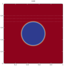
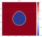
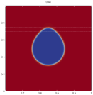
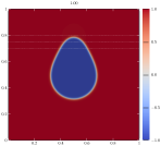
Figure 2: Contour plot of $\hat{\phi}^{n}$ showing the nucleation and expansion of a bleb over non-dimensional time with surface tension $\gamma=5\cdot 10^{-11}\mathrm{J}\,\mathrm{m}^{-2}$.

We consider a reduced species evolution law (20f), (20g): the density $\hat{{\rho}_{i}}^{\negthinspace n}$ is exchanged with $\hat{{\rho}_{i}}^{\negthinspace n}=\rho_{0}-\hat{{\rho}_{a}}^{\negthinspace n}$ for a total density of $\rho_{0}=2\cdot 10^{19}\,\mathrm{m}^{-3}$ (which is the total density estimated in [5, p. 1881] and rescaled to three dimensions by dividing with $x_{r}$), and the linkers’ diffusivity is set to zero as well as the regeneration rate. In Figure 3(a), we see how the density of active linkers decreases while the bleb expands.

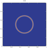
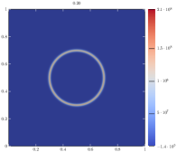
(a) Linker densities with $\gamma=5\cdot 10^{-11}~{}\mathrm{J}\,\mathrm{m}^{-2}$, force $\hat{f}=100~{}\mathrm{Pa}\,\mathrm{m}^{-1}$, total linker density $\rho_{0}=2.1\cdot 10^{9}~{}\mathrm{m}^{-3}$.

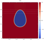
(b) Linker densities and corresponding membrane deformations with $\gamma=5\cdot 10^{-9}~{}\mathrm{J}\,\mathrm{m}^{-2}$, force $\hat{f}=500~{}\mathrm{Pa}\,\mathrm{m}^{-1}$, total linker density $\rho_{0}=2.5\cdot 10^{5}~{}\mathrm{m}^{-3}$.

Figure 3: Linker disconnection during bleb expansion.

Since we do not include a barrier where the cortex is, the membrane is slightly pulled inwards when the bleb forms at its northern front thus we have linker disconnection everywhere. However, the linker disconnection at the site where the bleb develops is strongest. To make this effect eminently visible, we also simulated the same situation with a higher force, see Figure 3(b).

Cortex Destruction

Let us turn to the second scenario. The homogeneous force density applied is the function in (21) without the first $\exp$ function factor. The surface tension is chosen as before. We consider active and inactive linkers without disconnection, but non-zero reconnection rate as in Table 1. In the course of time, we can see a membrane protrusion developing at the site where the cortex is damaged in Figure 4. It is interesting to note that the shape of the bleb is different from what we observed in Figure 2 by reaching approximately the same height. Also, the bleb expands about $40$ times faster, so for further studies one might reconsider the choice of the homogeneous force’s magnitude $\hat{f}$.

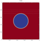
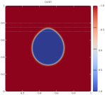
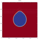
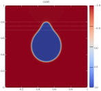
Figure 4: Bleb nucleation and expansion due to cortex destruction.

5 Conclusion

In this work, we presented a diffuse interface model for modelling the phenomenon of “cell blebbing”. We extended the existing theory by integrating several effects considered in distinct models separately into one three-dimensional model. The theoretical foundation of our modeling approach is Onsager’s variational principle. In our free energy, we incorporated the well-known Canham–Helfrich energy as well as a new generalized Hookean energy that accounts for the coupling of the cell membrane and the cell cortex via linker proteins that can also be interpreted as surfactants. An unconditionally energy stable numerical scheme for space and time discretization of the model with static cortex has been implemented. High computational costs introduced by non-local effects from the coupling have been mitigated by a hybrid parallel approach combining MPI multithreading. We then validated our modeling approach numerically by qualitatively reproducing behavior of cell blebs reported in biological literature.

The behavior of the protein linkers has been modeled on a pure mechanical basis in contrast to the dynamics of surfactants that “actively” participate in energy minimization. Investigations in this kind of models could shed light on new aspects of linker dynamics since to the best of the authors’ knowledge, they have never before been considered as surfactants.

To make simulation more feasible, it would be of high value to spare distributed memory parallelization. If the connectivity of the linkers is concentrated like in our proposed Gaussian model, the non-local integral terms can be approximated by local terms (concentrated on the diffuse layer of the cortex). An approach towards using this locality for sorting out large parts of the mesh efficiently during assembly might be a quadtree-organized mesh: modern GPUs provide dedicated hardware for traversing such data structures (e.g. RT Cores or Ray Accelerators).

References

• [1] H. Abels and H. Garcke, Weak solutions and diffuse interface models for incompressible two-phase flows, in Handbook of mathematical analysis in mechanics of viscous fluids, Springer, Cham, 2018, pp. 1267–1327.
• [2] H. Abels, H. Garcke, K. F. Lam, and J. Weber, Transport Processes at Fluidic Interfaces, Birkhäuser, 2017, ch. Two-Phase Flow with Surfactants: Diffuse Interface Models and Their Analysis, pp. 255–270.
• [3] S. Aland, A. Hahn, C. Kahle, and R. Nürnberg, Transport Processes at Fluidic Interfaces, Birkhäuser, 2017, ch. Comparative Simulations of Taylor Flow with Surfactants Based on Sharp- and Diffuse-Interface Methods.
• [4] R. Alert and J. Casademunt, Bleb nucleation through membrane peeling, Physical Review Letters, 116 (2016), https://doi.org/10.1103/physrevlett.116.068101.
• [5] R. Alert, J. Casademunt, J. Brugués, and P. Sens, Model for probing membrane-cortex adhesion by micropipette aspiration and fluctuation spectroscopy, Biophysical Journal, 108 (2015), pp. 1878–1886, https://doi.org/10.1016/j.bpj.2015.02.027.
• [6] J. Boss, Mitosis in cultures of newt tissues, Experimental Cell Research, 8 (1955), pp. 181–187, https://doi.org/10.1016/0014-4827(55)90055-0.
• [7] P. B. Canham, The minimum energy of bending as a possible explanation of the biconcave shape of the human red blood cell, Journal of theoretical Biology, 26 (1970), pp. 61–81, https://doi.org/10.1016/s0022-5193(70)80032-7.
• [8] H. D. Ceniceros, R. L. Nós, and A. M. Roma, Three-dimensional, fully adaptive simulations of phase-field fluid models, Journal of Computational Physics, 229 (2010), pp. 6135–6155, https://doi.org/10.1016/j.jcp.2010.04.045.
• [9] G. T. Charras, A short history of blebbing, Journal of Microscopy, 231 (2008), pp. 466–478, https://doi.org/10.1111/j.1365-2818.2008.02059.x.
• [10] G. T. Charras, M. Coughlin, T. J. Mitchison, and L. Mahadevan, Life and times of a cellular bleb, Biophysical Journal, 94 (2008), pp. 1836–1853, https://doi.org/10.1529/biophysj.107.113605.
• [11] G. T. Charras and E. Paluch, Blebs lead the way: how to migrate without lamellipodia, Nature Reviews Molecular Cell Biology, 9 (2008), pp. 730–736, https://doi.org/10.1038/nrm2453.
• [12] C. Dirks, P. Striewski, B. Wirth, A. Aalto, A. Olguin-Olguin, and E. Raz, A mathematical model for cell polarization in zebrafish primordial germ cells. 2019.
• [13] Q. Du, C. Liu, R. Ryham, and X. Wang, Modeling the spontaneous curvature effects in static cell membrane deformations by a phase field formulation, Communcations on Pure and Applied Mathematics, 4 (2005), pp. 537–548, https://doi.org/10.3934/cpaa.2005.4.537.
• [14] O. R. A. Dunbar, K. F. Lam, and B. Stinner, Phase field modelling of surfactants in multi-phase flow, Interfaces Free Bound., 21 (2019), pp. 495–547, https://doi.org/10.4171/ifb/429, https://doi.org/10.4171/ifb/429.
• [15] E. Evans, Probing the relation between force—lifetime—and chemistry in single molecular bonds, Annual Review of Biophysics and Biomolecular Structure, 30 (2001), pp. 105–128, https://doi.org/10.1146/annurev.biophys.30.1.105.
• [16] H. Garcke, K. Lam, and B. Stinner, Diffuse interface modelling of soluble surfactants in two-phase flow, Communications in Mathematical Sciences, 12 (2014), pp. 1475–1522, https://doi.org/10.4310/cms.2014.v12.n8.a6.
• [17] M. Goudarzi, K. Tarbashevich, K. Mildner, …, M. Bagnat, T. Betz, and E. Raz, Bleb expansion in migrating cells depends on supply of membrane from cell surface invaginations, Developmental Cell, 43 (2017), pp. 577–587, https://doi.org/10.1016/j.devcel.2017.10.030.
• [18] F. Guillén-González and G. Tierra, Unconditionally energy stable numerical schemes for phase-field vesicle membrane model, Journal of Computational Physics, 354 (2018), pp. 67–85, https://doi.org/10.1016/j.jcp.2017.10.060.
• [19] W. Helfrich, Elastic properties of lipid bilayers: Theory and possible experiments, Zeitung für Naturforschung, 28 (1973), pp. 693–703, https://doi.org/10.1515/znc-1973-11-1209.
• [20] L. D. Landau and E. M. Lifshitz, Fluid Mechanics, vol. 6 of Course of Theoretical Physics, Pergamon Press, Oxford, 2 ed., 1987.
• [21] S. M. Laster and J. M. Mackenzie, Bleb formation and f-actin distribution during mitosis and tumor necrosis factor-induced apoptosis, Microscopy Research and Technique, 34 (1996), pp. 272–280, https://doi.org/10.1002/(sici)1097-0029(19960615)34:3<272::aid-jemt10>3.0.co;2-j.
• [22] L. M. Lee and A. P. Liu, The application of micropipette aspiration in molecular mechanics of single cells, Journal of Nanotechnology in Engineering and Medicine, (2014), p. Article 040801, https://doi.org/10.1115/1.4029936.
• [23] F. Y. Lim, K.-H. Chiam, and L. Mahadevan, The size, shape, and dynamics of cellular blebs, Europhysiscs Letters, 100 (2012), 28004, https://doi.org/10.1209/0295-5075/100/28004.
• [24] L. Modica, The gradient theory of phase transitions and the minimal interface, Archive for Rational Mechanics and Analysis, 92 (1987), pp. 123–142.
• [25] L. Modica and S. Mortola, Un esempio di $\gamma$-convergenza, Bollettino dell’Unione Matematica Italiana B, 14 (1977), pp. 285–299.
• [26] Y. Nagase and Y. Tonegawa, A singular perturbation problem with integral curvature bound, Hiroshima Mathmetical Journal, 35 (2007), pp. 455–489, https://doi.org/10.32917/hmj/1200529813.
• [27] N. Nakatsuji, M. H. L. Snow, and C. C. Wylie, Cinemicrographic study of the cell movement in the primitive-streak-stage mouse embryo, Journal of Embryology and Experimental Morphology, 96 (1986), pp. 99–109, https://doi.org/10.1242/dev.96.1.99.
• [28] J. Prüss and G. Simonett, Moving Interfaces and Quasilinear Parabolic Evolution Equations, vol. 105 of Monographs in Mathematics, Birkhäuser, 2016, https://doi.org/10.1007/978-3-319-27698-4.
• [29] M. Röger and R. Schätzle, On a modified conjecture of de giorgi, Mathematische Zeitschrift, 254 (2006), pp. 675–714, https://doi.org/10.1007/s00209-006-0002-6.
• [30] S. A. Safran, N. Gov, A. Nicolas, U. S. Schwarz, and T. Tlusty, Physics of cell elasticity, shape and adhesion, Physica A, 352 (2005), pp. 171–201, https://doi.org/10.1016/j.physa.2004.12.035.
• [31] J. Schöberl, C++11 implementation of finite elements in ngsolve, tech. report, Institute for Analysis and Scientific Computing, TU Wien, 2014. https://www.asc.tuwien.ac.at/~schoeberl/wiki/publications/ngs-cpp11.pdf.
• [32] U. Seifert, Configurations of fluid membranes and vesicles, Advances in Physics, 46 (1997), pp. 13–137, https://doi.org/10.1080/00018739700101488.
• [33] I. Steinbach, Phase-field models in materials science, Modelling and Simulation in Materials Science and Engineering, 17 (2009), 073001, https://doi.org/10.1088/0965-0393/17/7/073001.
• [34] B. Stinner, A. Dedner, and A. Nixon, A finite element method for a fourth order surface equation with application to the onset of cell blebbing, Frontiers in Applied Mathematics and Statistics, 6 (2020), p. Article 21, https://doi.org/10.3389/fams.2020.00021.
• [35] W. Strychalski, C. A. Copos, O. L. Lewis, and R. D. Guy, A poroelastic immersed boundary method with applications to cell biology, Journal of Computational Physics, 282 (2015), pp. 77–97, https://doi.org/10.1016/j.jcp.2014.10.004.
• [36] W. Strychalski and R. D. Guy, A computational model of bleb formation, Mathematical Medicine and Biology, 30 (2013), pp. 115–130.
• [37] J. P. Trinkhaus, Formation of protrusions of the cell surface during tissue cell movement, Progress in clinical and biological research, 41 (1980), pp. 887–906.
• [38] P. Werner, Sharp and diffuse interface models for the evolution of surfaces that are immersed in fluids and coupled through surfactants, phd thesis, Friedrich-Alexander Universität Erlangen-Nürnberg, 2021.
• [39] P. Werner, M. Burger, and H. Garcke, Formal asymptotic analysis of a diffuse interface model for cell blebbing with linker dynamics. in preparation, 2021.
• [40] P. Werner, M. Burger, and J. Pietschmann, A pde model for bleb formation and interaction with linker proteins, Transactions of Mathematics and its Applications, 4 (2020), 1, https://doi.org/10.1093/imatrm/tnaa001.
• [41] M. Yao, B. T. Goult, B. Klapholz, X. Hu, C. P. Toseland, Y. Guo, P. Cong, and J. Sheetz, M. P. Yan, The mechanical response of talin, Nature Communications, 7 (2016), 11966, https://doi.org/10.1038/ncomms11966.