Multi-variance replica exchange stochastic gradient MCMC for inverse and forward Bayesian physics-informed neural network
Abstract
Physics-informed neural network (PINN) has been successfully applied in solving a variety of nonlinear non-convex forward and inverse problems. However, the training is challenging because of the non-convex loss functions and the multiple optima in the Bayesian inverse problem. In this work, we propose a multi-variance replica exchange stochastic gradient Langevin diffusion method to tackle the challenge of the multiple local optima in the optimization and the challenge of the multiple modal posterior distribution in the inverse problem. Replica exchange methods are capable of escaping from the local traps and accelerating the convergence; two chains with different temperatures are designed where the low temperature chain aims for the local convergence, and the target of the high temperature chain is to travel globally and explore the whole loss function entropy landscape. However, it may not be efficient to solve mathematical inversion problems by using the vanilla replica method directly since the method doubles the computational cost in evaluating the forward solvers (likelihood functions) in the two chains. To address this issue, we propose to make different assumptions on the energy function estimation and this facilities one to use solvers of different fidelities in the likelihood function evaluation. More precisely, one can use a solver with low fidelity in the high temperature chain while use a solver with high fidelity in the low temperature chain. Our proposed method significantly lowers the computational cost in the high temperature chain, meanwhile preserves the accuracy and converges very fast. We give an unbiased estimate of the swapping rate and give an estimation of the discretization error of the scheme. To verify our idea, we design and solve four inverse problems which have multiple modes. The proposed method is also employed to train the Bayesian PINN to solve the forward and inverse problems; faster and more accurate convergence has been observed when compared to the stochastic gradient Langevin diffusion (SGLD) method and vanila replica exchange methods.
keywords:
MCMC, Langevin diffusion, replica exchange, stochastic gradient descent, inverse problem, Bayesian physics-informed neural network1 Introduction
The development of deep neural networks (DNNs) has drawn people’s attention to incorporate Bayesian approach into the learning of DNNs [1, 33, 12]. Stochastic gradient Markov chain Monte Carlo methods [33, 14, 20, 18, 4, 25] have become attractive due to its potential for uncertainty quantification applications. In this family of approaches, the stochastic gradient Langevin dynamics [33] algorithm was first proposed which bridges the gap between optimization and Bayesian inference.It was originates from the discretization of Langevin diffusion, but uses small batches to approximate the true gradients. The updating formula of SGLD resembles that of stochastic gradient descent (SGD), thus it can be naturally used in deep learning tasks with large datasets and is easy to implement in practice. By injecting a judicious choice of noise when updating the DNN parameters, the method ensures that the generated samples will converge to the true posterior instead of the MAP [33, 29, 2].
Many variants of stochastic gradient MCMC methods have also been proposed to improve the convergence or stability of SGLD. In the case when the parameters of the DNN have complicated posterior density [10, 14, 4] such as different scales of variance or highly correlated, some preconditioning methods were introduced taking into account the geometric information. These include the preconditioned SGLD, Hessian approximated SGMCMC [14, 25, 18, 32, 31], where some preconditioners are proposed to approximation the Hessian information of the log posterior. Other improvements include the high-order integrators in the discretization of Langevin diffusion [3], for example, stochastic gradient Hamiltonian Monte Carlo [4], stochastic gradient thermostats [12]. To combine simulated tempering with the traditional MCMC community, a replica stochastic gradient MCMC (reSG-MCMC) was recently brought up [11].
The main idea of the standard replica exchange Langevin dynamics is to use multiple diffusion processes with different temperatures. The low temperature diffusion process can exploit the local area, and the high temperature one will explore the global domain. With a suitable swapping criteria, the replica exchange method admits a trade-off between global exploration and local exploitation, which accelerates the convergence rate of the samples to the invariant correct distribution. It is feasible and can be naturally extended for parallel computing. However, it is important to propose a good swapping scheme which aims to overcome the issue of large bias introduced by using mini-batches. In [11], the authors proposed an adaptive replica exchange SG-MCMC method with the help of stochastic approximation, which has a correction term to reduce the bias from the swaps based on theoretical analysis.
Compared to the other MCMC sampling methods, the replica exchange methods have the fast convergence property. However, it usually requires a higher computational cost due to the replica computation high temperature chain. To be specific, take as an example solving inverse physical problems under the Bayesian framework with efficient sampling algorithms, which has been a favored approach in the last century [27]. In the Bayesian approach, one treats the network weight parameters as random variables and infers them conditioned on limited data. The likelihood function consists of the loss between the the network output and observation data. For most of the physical problems, the computation of the loss involves the evaluation of the forward solver which maps the inverse target to the observations. Due to the mathematical properties of the equations, such as problems with multiscale nature, this can be a very time consuming process [13, 7]. Hence, there should be a balance between the fast convergence and high computational cost, and a modification to accelerate the computation of two likelihood (energy) functions in the two chains is needed.
Our idea is to overcome the difficulty by applying a coarser solver in the high temperature chain to explore the model parameter space. The motivation is that the high temperature chain is designed to guide the particle travel globally and escape from the local optimum trap, and it is practical to use a computational efficient coarse solver with little sacrifice on the accuracy. Since the errors in the forward solver and the other sources of errors contribute to the energy function estimation, one needs to make different assumptions on the energy functions in the two chains. To the extent of our knowledge, this work is the first to study the theoretical and practical applications based on this idea.
The key contributions of this work are
-
1.
We introduce a multi-variance replica exchange method for Bayesian physics-informed neural networks. Adopting different variances for the energy function estimators in different diffusion processes allows us to take advantage of different model fidelities to perform numerical simulations.
-
2.
We derive a correction term to ensure the reduction of bias in the swapping scheme and prove the discretization error of the method.
-
3.
The proposed multi-variance replica exchange method is feasible in general Bayesian learning tasks. In particular, we use it in training the Bayesian PINN (physics-informed neural network). More precisely, physical laws are integrated in the deep neural network by the constraints in the loss; and we use noisy training data, and the outcome of the network can provide uncertainties of the prediction.
-
4.
The proposed method is applied to solve both forward and inverse PDE problems. The numerical results demonstrate the improved efficiency in capturing both multiple modes and infinite modes in some inverse problems. It also shows the better predictions and faster convergence with reliable uncertainties in solving PINN problems when compared to the classical gradient based methods.
The outline of the paper is as follows. In Section 2, we review some backgrounds in stochastic gradient Langevin dynamics, replica exchange stochastic gradient MCMC algorithms, and Bayesian framework for inverse problems 3. Our main algorithm is presented in Section 4. Numerous numerical examples are shown to illustrate the efficiency of proposed method in Section 5.
2 Preliminaries
2.1 Replica exchange Langevin diffusion (reLD)
Diffusion-based Markov Chain Monte Carlo (MCMC) algorithms have become increasingly popular in the recent years due to the real applications performance and theoretic supports [19, 24, 26, 21]. One of the most popular choices is the Langevin diffusion which is a stochastic differential equation as follows:
| (1) |
Here , is called temperature; is the standard Brownian motion in . is the energy function which is often convex. Denote by the train data, where is a data point, one choice of the energy function is:
| (2) |
where and is the prior and is the likelihood. People have established that under mild conditions, the solution process will converge to the invariant distribution [23, 19]. However, when the temperature is large, the flattened distribution is less concentrated around the global optimum and the geometric connection to the global minimum is affected [21]. As a result, the particle is exploring the whole loss function landscape and can travel globally [36]. On the other hand, a low-temperature results in the exploitation: the particle is exploiting the local region; the local optima can be reached quickly; however, the particle is hard to escape from the local trap (local optima) which is harmful for the global convergence [11].
This motivates people designing the mixed algorithm; the replica exchange Langevin diffusion (reLD) is then designed. In this algorithm, two chains with different temperatures are used,
People can switch the particles between two chains. More precisely, let be a constant and if one follows the swapping rate , , where,
| (3) |
the system then converges to the invariant distribution; the density is given as follow:
| (4) |
2.2 Stochastic Gradient Langevin Dynamics (SGLD)
The MCMC aalgorithm can can be used as an optimization algorithm. Consider the discretization of (1),
| (5) |
where solves the equation; is a constant and can be understood as the learning rate; is a standard d-dimensional Gaussian vector. Equation (5) is a stochastic gradient descent (SGD) algorithm with some perturbations, the discretized equation returns to the gradient descent algorithm when . The connection between Langevin MCMC and the gradient descent has been recently established in [9, 26] for strongly convex . Moreover, [21, 34] proved non-asymptotic guarantees for this perturbed scheme. In real applications, is large and the likelihood function is hard to evaluate [13, 7], this brings difficult in calculating the energy function; hence the approximation is often used and this will result in an error in the convergence. Furthermore, in physical applications, calculating the likelihood usually involves evaluating the forward solver, which also contributes an error in the convergence. In the theoretical analysis, if we denote as the estimator of the energy function, people usually assume that
| (6) |
where is the variance and is the reflection of the error.
Motivated by the stochastic gradient descent algorithm (SGD), people can build an estimator of the energy function with a random subset of samples. More precisely,
| (7) |
where is the index of a batch of samples. We hence have the stochastic gradient Langevin diffusion (SGLD),
| (8) |
In [28], the authors have shown that SGLD asymptotically converges to a unique invariant distribution.
2.3 Replica Exchange Stochastic Gradient Langevin Dynamics (reSGLD)
In the previous section, we have introduced the reLD and the optimization algorithm constructed using the Langevin diffusion. It is then natural to use the reLD to build an optimization algorithm, the reSGLD is then proposed. The discretization is the same as the SGLD and we have,
| (9) | |||
| (10) |
where are the temperatures, are the corresponding solutions. By following the estimation (6) and allowing swapping, i.e., with a rate which is an unbiased estimation111It should be noted that the original swapping rate (3) becomes bias due to the stochastic approximation of the energy function. of (3):
The authors theoretically give the discretization error of the scheme and the numerical results also surpass the benchmarks of several datasets.
3 Bayesian Framework of the Inversion Problems
One can solve the inverse problem using the Bayesian framework. A favored approach is to sample the inverse target by some MCMC algorithm. Let the observation of the problem be and the quantity of interest in the inverse problem be . The target is to generate samples that approximate the posterior . By the Bayes’ Theorem,
where is the prior and is the likelihood. The key in the implementation is to design and evaluate the likelihood function. This usually involves solving an forward problem given the proposal and measures the difference between the observation and the solution of the forward problem. In addition to the error in the forward solver, there are other sources of errors [13, 15] such as the errors in the real observation. One can assume the combined error follows a normal distribution with standard deviation , it follows that,
| (11) |
where denotes the forward solver and the can be viewed as the precision of the observations and the solver. There are two difficulties in practice. The first one is how to generate the proposals. This requires the design of the transition probability and one usually seeks ideas from the MCMC literature. One approach is to use the reinforcement learning to learn a transition probability function [7]. In this work, we are going to propose samples under the framework of Langevin dynamics. Another difficulty is the choice of forward solver. The simulation process is usually slow in particular if one requires high accuracy. Though Replica exchange method accelerates convergence in terms of the MCMC procedure, one still needs to run the forward solver several times due to its multi-chain property. This greatly increases the computational cost. Because of this limitation, the replica exchange method may not be directly applied to solve physical inverse problems. In this work, we propose a method which greatly reduces the computation time, and meanwhile preserves the fast convergence property of the replica exchange method.
4 Proposed Method
In this section we are going to present the proposed method. Replica exchange methods have been proved to capture the global optima successfully; however, it may be slow since we need to evaluate the likelihood functions twice in the low and high temperature chains separately. The problem becomes exacerbated in solving inversion physical problems in the Bayesian framework. This is because people need to evaluate an forward solver in calculating the likelihood functions, which is extremely time consuming; if we repeat the process twice, this will largely increase the computation time. People hence need to optimize the replica method to use it in real world problems.
The question is: do we need to use the same solver in calculating the energy functions in two chains? Our proposal is to use a fine solver in the chain with low temperature while applying a coarser solver in the high temperature chain which travels globally. The motivation of the proposed method is: the high temperature chain is exploring the region, its job is to get rid of the local optimum and find the potential region where the global optima lays in; it hence requires less accuracy. For the better convergence to the global optima, once the particle is closed to the region, we use the low temperature chain which has a fine solver for the better accuracy. Basing on this reasoning, we then can use a coarse solver in the high temperature chain and assume a larger variance in the energy estimation. Our experiments show that the accuracy will not be compromised and we prove that the discretization error will not be changed. We hence can benefit from the computation cost saved in the coarse solver evaluation.
As we have discussed in the last section, the solver contributes errors in the energy functions; together with error in the stochastic gradients one may assume that the estimations satisfies, for example, (6). We propose to use different solvers; this means that the energy function estimations are different, hence a new swapping rate should be derived. Now let denote the solution of the proposed scheme, the scheme can be summarized as follow,
| (12) | |||
| (13) |
where and are the two estimators. We denote as the continuous solution with the different estimator, then the new estimator is summarized in the following theorem.
Theorem 4.1.
Let and satisfies ; set for and denote . Then the estimator:
| (14) |
is unbiased.
Proof.
By the assumption on and we have,
where can be taken as a Brownian motion when which is a Gaussian vector. The switching rate for is then given and simplified as follow:
The partial derivatives of are straightforward as follow,
Ito’s lemma then reads,
Thus is Martingale. Set , the desired estimator is unbiased. ∎
4.1 Discretization Error
In this section, we comment on the discretization error of the proposed method. We first introduce the strong form solution which satisfies:
| (15) |
Here , and is the energy function. is a Brownian motion and is a stochastic process which switches between and with the probability ; here denotes the identity matrix and is given in (3).
Let us denote as the solution of the full discretization scheme; that is, satisfies,
| (16) |
where is a fix time step and is a standard Gaussian distribution. is a stochastic process and switches between and with the probability . is defined the same as but is switching with the . We also define the semi-discretized solution as the linear interpolation of which satisfies,
| (17) |
Here denotes the floor function and follows the same trajectory as . To prove the discretization theorem. Two assumptions on the energy functions should be made. We first assume that the energy function is smooth, more precisely, there exists such that for every , we have:
| (18) |
We also assume the dissipativity of the energy function. That is, there are constants and such that
| (19) |
true for all and denotes the inner product. We also quantify the errors in the swapping rate and energy function estimator; that is, we have and , where and are in and are the functions measuring the error in the swapping rate and energy function estimations at iteration.
Theorem 4.2.
If we have the smoothness and dissipative assumptions, and we further assume that satisfies , then there exist constants such that,
| (20) |
where depends on the temperatures , the dimension of , the finite time and the other constants in the assumptions (18) and (19); and depends on and ; depends on which defines the swapping rate, and . We give an outline of the proof and please refer to [11, 5] for the details.
Proof.
Integrate (15) from to and substract (17), if we assume that , we then have,
| (21) |
where denotes the floor function. Take expectation over , it then follows that:
| (22) |
note that the above inequality is estimated due to the Burkholder-Davis-Gundy and Cauchy-Schwarz inequalities. We play the trick of triangle inequality; more precisely, for any where is an integer, we have,
and for we have,
where is the continuous-time interpolation of without noise and satisfies the following equation:
We can estimtae and separately and the theorem can be proved. ∎
5 Numerical Examples
In this section, we will demonstrate the performance of the proposed methods, multi-variance replica exchange Langevin diffusion (m-reSGLD), by a sequence of numerical experiments. In section (5.1), an inverse problem will be presented; and the experiments are designed to show that the proposed approaches are able to capture the multiple modes. In the rest of the numerical experiments sections, we will use the proposed methods as an optimization algorithm; in particular, we will consider several partial diffusion equations (PDEs) in the physics-informed neural network (PINN) framework.
5.1 Experiment 1
In this section, we will study an inverse problem which is commonly studied in the water resources research [16]. The problem can be solved by the sampling methods in the Bayesian framework. Compared to the traditional gradient based methods, the proposed methods converges faster and are able to capture the multiple modes (multiple inverse quantity of interests, or, multiple modal posteriors from the Bayesian perspective). This is the consequence of the information exchange between the low temperature chain and high temperature chain. We consider the following parabolic equation which models the contamination flows in the water:
| (23) | |||
| (24) | |||
| (25) |
In the above formulation, ; is the Euclidean distance. and are two positive constants; where can be taken as the radius of the pollution source and is the strength of the initial contamination. In the following two experiments, we set and . The initial condition is partially given; more precisely, the pollution source is unknown. The target of the experiments is to trace back the initial pollution source given some observation data which are the concentration at some sensors in the domain.
We set the solution of the forward problem to be . We will perform two experiments; the first experiment has 2 inverse solutions and the second one has infinite number of solutions. In both experiments, we apply the standard finite element solver. To be more specific, we are going to use a finer finite element solver with in the low temperature chain which reinforces the local convergence; while in the high temperature chain which is easier to travel globally, we use a coarser finite element solver with . The time differences for both experiments are set to be .
5.1.1 Two inverse solutions
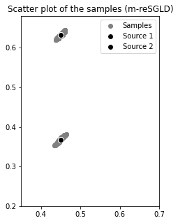
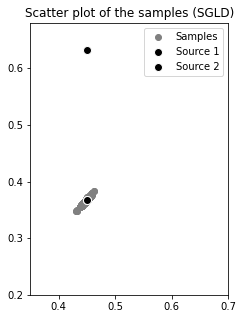
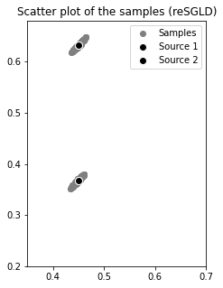
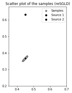
Two sensors are placed at and and sensors measure the concentration (solution) of the pollution at the terminal time ; in our experiment, , where . This setting guarantees to have 2 inverse solutions. In order to show the efficiency and accuracy of the proposed method, we will compare the method, namely the multi-variance replica exchange Langevin diffusion (m-reSGLD), with the single chain SGLD and the same energy function reSGLD. That is, the first comparison test is the standard single chain SGLD; while we are going to use the same fine solver () in both chains in the latter reSGLD method.
In Figure (1), m-reSGLD and reSGLD are run with 30,000 iterations while SGLD is run with 60,000 iterations. We can observe from the picture (1) that the proposed method can capture both pollution sources while the single chain method fails to capture the other source. The reSGLD with the same solver (right picture) also can capture the multimodes as expected; in fact, this method should be the most accurate one; however, since we use the same fine solver in both chains, the computational cost is extremely high. In our tests, the proposed method runs around while the fine solver method runs on the computing resource.
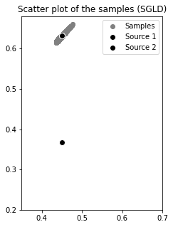
We also conduct the experiments using three methods but fixing the same computation time, i.e., the running time of all three methods are the same. We can see that the m-reSGLD can still capture the multiple modes; however, the reSGLD is unable to achieve the goal. The reason is: it takes a long time to evaluate 2 fine forward solvers (in both chains) and the computation terminates with not enough number of iterations. The results are shown in Figure (2).

We want to comment on the accuracy of the solver used in the high temperature chain. There is a trade-off of the accuracy and the computational cost. More precisely, using a high accuracy solver can increase the accuracy; however, this will increase the computational cost and then limits the number of iterations of the algorithm.
5.1.2 Infinite inverse solutions
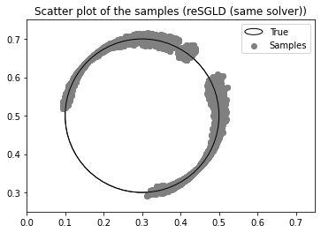
To generate infinite number of solutions, we only place one sensor at position , we still measure the concentration at the terminal time and use the same value as before. It is not hard to see that: the inverse target is a circle centered at the sensor and the underlying problem has infinite number of solutions. Same as the first experiment, we will compare our method with 2 other methods.
In the first set of experiments, which is shown in Figure (3), three algorithms are run with 60000 iterations. We can see that from the Figure (3) that, the proposed method greatly improves the sampling when compared to the single chain SGLD. The reSGLD method with the same energy method also works well; however, the computation time is around while our proposed method only takes around to finish generating the same number of samplings (iterations).
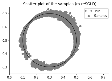
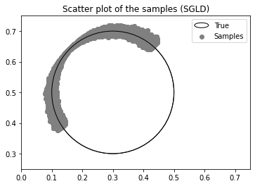
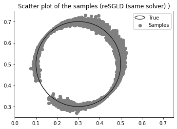
We also fix the computation time and compare the three methods, the results are demonstrated in Figure (4). We can see that m-reSGLD still performs well and is the best among the three methods. In first set of experiments, the reSGLD is able to capture the multimodes; however, if the running time is the same with that of m-reSGLD, reSGLD performance is compromised. This is due to the heavy computations of two fine forward solvers; as a result, training iterations are not enough.

5.2 Bayesian Physics-informed neural network (PINN)
Starting from this experiment, we are going to apply the proposed methods as an optimization approach in the neural network. In particular, we will solve three PDEs in both forward and inverse settings with the physics-informed neural network (PINN) [22].
To learn the solutions for a given PDE with limited data, such as boundary/initial conditions and information about the source term, it is important to incorporate the available physical equations/laws in the design of deep neural networks. Physics-informed neural networks (PINN) [17, 35, 22] were proposed to realize the idea and have been successfully applied to many forward and inverse PDE applications subject to the law of physics that governs the data. Given a PDE of the form
where is a differential operator and is the boundary condition operator. is the computational domain and is the source term, is the boundary condition. Denote by the neural network parameterized by , the PINN aims to minimize the mean squared loss
| (26) |
where are the positive weights.
However, it was shown that the training of PINN is very challenging for PDEs, due to significantly the multiple local optima in the loss function and varying gradients in the back-propagation [30]. Moreover, for the case when the data has noise, standard PINNs do not naturally have the capability to capture uncertainties. Recently, a Bayesian physics-informed neural network framework [35] is proposed to deal with the issue. The Bayesian neural network differs from classical neural network by inducing a probability distribution on the model parameters of the network. This allows to estimate uncertainties in the predictions. Assume that the solution, source and boundary data has some noises,
where follow Gaussian distribution with zero mean, and standard deviation , respectively. Given data , and , , , the likelihood is defined to be ,
The posterior distribution is then . For the posterior inference, the variational inference method and some variants of MCMC methods are commonly used.
In this work, we adopt the replica exchange stochastic gradient MCMC approach. It stems from stochastic gradient Langevin dynamics (SGLD) , and is a simulated tempering approach which can accelerate the training and guarantees a better global point estimate.
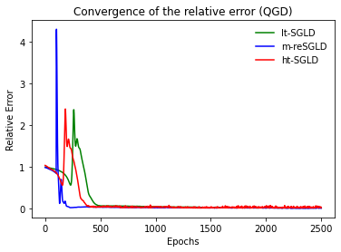
5.3 Experiment 3 (Quasi-gas dynamics (QGD))
We solve a quasi-gas dynamics (QGD) model which is a kinetic equations under the assumption that the distribution function is similar to a locally Maxwellian representation. The QGD model is extensively studied and is not easy to be solved by the numerical methods [6, 8]; and we hence propose to solve it by the deep learning methods. Consider the QGD equation in a polygonal domain ():
| (27) |
Here, is the terminal time and is a positive constant which measures the diffusion effect, is conductivity of the model and is strictly positive, is the source of the equation with a proper regularity. Furthermore, we assume that the initial conditions and . In our experiments, and . We set the solution to be and the initial conditions and source can be derived then.
In this work, and . We design a four layer fully connected neural network () activated by the function. points are uniformly placed in in the low temperature chain and to accelerate the computation, points are used in the high temperature chain. In both chains, we use points in time including the initial condition to discretize the time direction.
To demonstrate the performance of our method, we will compare the proposed method (m-reSGLD) with the single chain method, i.e., SGLD without the replica exchange. We will run the SGLD for two times: a low temperature SGLD (lt-SGLD) and a high temperature SGLD (ht-SGLD) respectively. To be more specific, the temperature in lt-SGLD is set to be the same as the low temperature in the m-reSGLD; meanwhile, the temperature in ht-SGLD is is set to be the same as the high temperature in the m-reSGLD. The relative convergence is shown in Figure (5) and the mean and variance of the relative errors of the three methods are shown in Table (1).
| Methods | Mean of the relative error | Variance of the relative error |
|---|---|---|
| m-reSGLD | 0.01918168 | 2.324e-05 |
| lt-SGLD | 0.02376848 | 0.00033714 |
| ht-SGLD | 0.03477052 | 0.00014472 |
From Figure (5) and Table (1), we can observe that the proposed method (blue curve) decays very fast, in particular when compared to the low temperature SGLD (green curve). The high temperature SGLD also has a quick convergence at the beginning since the high temperature encourages the global travel and the particle may move to the global optimal point earlier; however, the relative error of the ht-SGLD is the largest at the end and the blue curve (proposed m-reSGLD) stabilizes with the lowest relative error. Intuitively, this is due to the better local convergence of the low temperature SGLD.
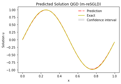
We also plot the solution of the last time step in Figure (6) as reference.
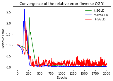
5.4 Experiment 4 (Inverse QGD)
In this section, we are going to consider the QGD equation again but in the inverse setting, that is, is not given and we will learn this constant together with the solution of the equation. The network is kept the same as before except that the last layer is of size . We need additional observation information and hence use 10 true solution points equally spaced. The relative convergence is shown in Figure (7) and the mean and variance of the relative errors of the three methods are shown in Table (2).
| Methods | Mean of the relative error | Variance of the relative error |
|---|---|---|
| m-reSGLD | 0.02559266 | 0.00019022 |
| lt-SGLD | 0.04922535 | 0.00071017 |
| ht-SGLD | 0.15169148 | 0.00552021 |
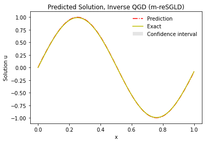
From Table (2) and Figure (7), we observe the similar results as before. The proposed method (m-reSGLD) demonstrates a faster convergence and stabilizes with a smaller relative error. We also plot the the solution of the last time step in Figure (8).
Besides the convergence of the solution, we also present the prediction of the inverse target . Please check Table (3) for the details. We can observe that the proposed method gives us the best solution.
| Methods | True | Mean of | Variance of |
|---|---|---|---|
| m-reSGLD | 1.0 | 1.0033238 | 1.9756535e-05 |
| lt-SGLD | 1.0 | 1.0096047 | 0.0001136835 |
| ht-SGLD | 1.0 | 0.9906514 | 0.0001133237 |
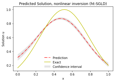
5.5 Experiment 2 (Nonlinear Inverse)
We consider an inverse PINN problem as fellow:
| (28) | |||
| (29) |
where is a constant and will be derived according to the pre-set solution. In this example, solution is set to be and the true . The target is to learn the solution and find at the same time. We design a four-layer fully connected neural network () activated by the function. points are uniformly placed for training in in the low temperature chain and to accelerate the computation, points are used in the high temperature chain. For the observation, we place 5 sensors uniformly to measure the solutions of the equation.
In order to show the fast convergence and the low variance. We are going to compare our method (m-reSGLD) with the SGLD without exchange. The temperatures of the single chain methods are set to be same with the low and high temperature in the proposed method respectively. More precisely, in Figure (9), the red curve, high-temperature SGLD (ht-SGLD), is the convergence of the relative error of the SGLD method with a temperature the same as the high temperature used in the proposed m-reSGLD (blue curve). The green curve, low-temperature SGLD (lt-SGLD), is the convergence of the relative error of the SGLD method with a temperature the same as the low temperature used in the proposed m-reSGLD. The convergence of the method is demonstrated in Figure (9); the mean and variance of the relative errors are shown in Table (4).
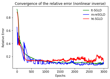
From the Figure (9), we can observe that the blue curve (m-reSGLD) has a fast decay and converges to the lowest relative error. The fast decay can be intuitively explained: the high chain is exploring and once it is close to the optimal points, the likelihood then becomes large, which results in a bigger swapping rate (14). This mechanism will help the particle explore the whole loss function landscape and accelerate the convergence.
| Methods | Mean of relative error | Variance of relative error |
|---|---|---|
| m-reSGLD | 0.07956814 | 8.962e-05 |
| lt-SGLD | 0.09911878 | 5.032e-05 |
| ht-SGLD | 0.15661082 | 0.00074168 |
The mean and variance of the predicted are shown in Table (5).
| Methods | True | Mean of | Variance of |
|---|---|---|---|
| m-reSGLD | 0.7 | 0.6679792 | 0.001696 |
| lt-SGLD | 0.7 | 0.6406617 | 0.000534 |
| ht-SGLD | 0.7 | 0.8007492 | 0.002135 |
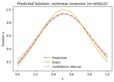
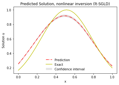
The sample solutions are demonstrated in Figure (10).
6 Conclusion
The traditional replica exchange method assumes that the energy function estimates are the same; this means that in the Bayesian framework of solving inverse problems, one can only use the same solver in both chains; this results in a high computational cost. In this work, we generalize the replica exchange method with different energy function estimates. To be more specific, people can use a fine resolution solver in the low temperature chain while applying a coarse resolution solver in the high temperature chain. We hence use forward solvers with different fidelities; this setting can save a lot of computational cost in the high temperature chain and is much more efficient when compared to the single fidelity solver method while maintaining the accuracy. We give an unbiased swapping rate and give an estimation of the discretization error. At the end, we verify that our method can capture the multiple-mode non-Gaussian posterior distribution in the Bayesian inverse problems; the examples demonstrate that our methods can beat the classical methods both in terms of the efficiency and accuracy. We also apply the method as an sampling algorithm and solve several forward and inverse mathematical problems in the physics-informed neural network framework. Compared to the classical methods, our method reduces the relative error of the solutions for the forward problems and the error of the inverse quantity of interests for the inversion problems.
References
- [1] S. Ahn, A. Korattikara, and M. Welling. Bayesian posterior sampling via stochastic gradient fisher scoring. arXiv preprint arXiv:1206.6380, 2012.
- [2] C. Chen, N. Ding, and L. Carin. On the convergence of stochastic gradient mcmc algorithms with high-order integrators. In Advances in Neural Information Processing Systems, pages 2278–2286, 2015.
- [3] C. Chen, N. Ding, and L. Carin. On the convergence of stochastic gradient mcmc algorithms with high-order integrators. In Advances in Neural Information Processing Systems, 2015.
- [4] T. Chen, E. Fox, and C. Guestrin. Stochastic gradient hamiltonian monte carlo. In International conference on machine learning, pages 1683–1691, 2014.
- [5] Y. Chen, J. Chen, J. Dong, J. Peng, and Z. Wang. Accelerating nonconvex learning via replica exchange langevin diffusion. arXiv preprint arXiv:2007.01990, 2020.
- [6] B. Chetverushkin, E. Chung, Y. Efendiev, S.-M. Pun, and Z. Zhang. Computational multiscale methods for quasi-gas dynamic equations. arXiv preprint arXiv:2009.00068, 2020.
- [7] E. Chung, Y. Efendiev, W. T. Leung, S.-M. Pun, and Z. Zhang. Multi-agent reinforcement learning accelerated mcmc on multiscale inversion problem. arXiv preprint arXiv:2011.08954, 2020.
- [8] E. Chung, Y. Efendiev, S.-M. Pun, and Z. Zhang. Computational multiscale methods for parabolic wave approximations in heterogeneous media. arXiv preprint arXiv:2104.02283, 2021.
- [9] A. Dalalyan. Further and stronger analogy between sampling and optimization: Langevin monte carlo and gradient descent. In Conference on Learning Theory, pages 678–689. PMLR, 2017.
- [10] Y. N. Dauphin, R. Pascanu, C. Gulcehre, K. Cho, S. Ganguli, and Y. Bengio. Identifying and attacking the saddle point problem in high-dimensional non-convex optimization. In Advances in neural information processing systems, pages 2933–2941, 2014.
- [11] W. Deng, Q. Feng, L. Gao, F. Liang, and G. Lin. Non-convex learning via replica exchange stochastic gradient mcmc. In International Conference on Machine Learning, pages 2474–2483. PMLR, 2020.
- [12] N. Ding, Y. Fang, R. Babbush, C. Chen, R. Skeel, and H. Neven. Bayesian sampling using stochastic gradient thermostats. In Advances in Neural Information Processing Systems, 2014.
- [13] Y. Efendiev, T. Hou, and W. Luo. Preconditioning markov chain monte carlo simulations using coarse-scale models. SIAM Journal on Scientific Computing, 28(2):776–803, 2006.
- [14] C. Li, C. Chen, D. Carlson, and L. Carin. Preconditioned stochastic gradient langevin dynamics for deep neural networks. In Thirtieth AAAI Conference on Artificial Intelligence, 2016.
- [15] Q. Li and K. Newton. Diffusion equation-assisted markov chain monte carlo methods for the inverse radiative transfer equation. Entropy, 21(3):291, 2019.
- [16] W. Li and G. Lin. An adaptive importance sampling algorithm for bayesian inversion with multimodal distributions. Journal of Computational Physics, 294:173–190, 2015.
- [17] L. Liu, T. Zeng, and Z. Zhang. A deep neural network approach on solving the linear transport model under diffusive scaling. arXiv preprint arXiv:2102.12408, 2021.
- [18] Y.-A. Ma, T. Chen, and E. Fox. A complete recipe for stochastic gradient mcmc. In Advances in Neural Information Processing Systems, pages 2917–2925, 2015.
- [19] T. H. Nguyen, U. Simsekli, and G. Richard. Non-asymptotic analysis of fractional langevin monte carlo for non-convex optimization. In International Conference on Machine Learning, pages 4810–4819. PMLR, 2019.
- [20] S. Patterson and Y. W. Teh. Stochastic gradient riemannian langevin dynamics on the probability simplex. In Advances in neural information processing systems, pages 3102–3110, 2013.
- [21] M. Raginsky, A. Rakhlin, and M. Telgarsky. Non-convex learning via stochastic gradient langevin dynamics: a nonasymptotic analysis. In Conference on Learning Theory, pages 1674–1703. PMLR, 2017.
- [22] M. Raissi, P. Perdikaris, and G. E. Karniadakis. Physics-informed neural networks: A deep learning framework for solving forward and inverse problems involving nonlinear partial differential equations. Journal of Computational Physics, 378:686–707, 2019.
- [23] G. O. Roberts and O. Stramer. Langevin diffusions and metropolis-hastings algorithms. Methodology and computing in applied probability, 4(4):337–357, 2002.
- [24] U. Şimşekli. Fractional langevin monte carlo: Exploring lévy driven stochastic differential equations for markov chain monte carlo. In International Conference on Machine Learning, pages 3200–3209. PMLR, 2017.
- [25] U. Simsekli, R. Badeau, T. Cemgil, and G. Richard. Stochastic quasi-newton langevin monte carlo. In International Conference on Machine Learning, volume 43, pages 642–651, 2016.
- [26] U. Simsekli, L. Zhu, Y. W. Teh, and M. Gurbuzbalaban. Fractional underdamped langevin dynamics: Retargeting sgd with momentum under heavy-tailed gradient noise. In International Conference on Machine Learning, pages 8970–8980. PMLR, 2020.
- [27] A. M. Stuart. Inverse problems: a bayesian perspective. Acta numerica, 19:451–559, 2010.
- [28] Y. W. Teh, A. H. Thiery, and S. J. Vollmer. Consistency and fluctuations for stochastic gradient langevin dynamics. Journal of Machine Learning Research, 17, 2016.
- [29] S. J. Vollmer, K. C. Zygalakis, and Y. W. Teh. Exploration of the (non-) asymptotic bias and variance of stochastic gradient langevin dynamics. The Journal of Machine Learning Research, 17(1):5504–5548, 2016.
- [30] S. Wang, H. Wang, and P. Perdikaris. On the eigenvector bias of fourier feature networks: From regression to solving multi-scale pdes with physics-informed neural networks. Computer Methods in Applied Mechanics and Engineering, 384:113938, 2021.
- [31] Y. Wang, W. Deng, and G. Lin. An adaptive hessian approximated stochastic gradient mcmc method. Journal of Computational Physics, 432:110150, 2021.
- [32] Y. Wang, W. Deng, and G. Lin. Bayesian sparse learning with preconditioned stochastic gradient mcmc and its applications. Journal of Computational Physics, 432:110134, 2021.
- [33] M. Welling and Y. W. Teh. Bayesian learning via stochastic gradient langevin dynamicsn. In Proceedings of the 28th international conference on machine learning (ICML-11), pages 681–688, 2011.
- [34] P. Xu, J. Chen, D. Zou, and Q. Gu. Global convergence of langevin dynamics based algorithms for nonconvex optimization. arXiv preprint arXiv:1707.06618, 2017.
- [35] L. Yang, X. Meng, and G. E. Karniadakis. B-pinns: Bayesian physics-informed neural networks for forward and inverse pde problems with noisy data. Journal of Computational Physics, 425:109913, 2021.
- [36] Y. Zhang, P. Liang, and M. Charikar. A hitting time analysis of stochastic gradient langevin dynamics. In Conference on Learning Theory, pages 1980–2022. PMLR, 2017.