A New Multipoint Symmetric Secant Method with a Dense Initial Matrix

Abstract.

In large-scale optimization, when either forming or storing Hessian matrices are prohibitively expensive, quasi-Newton methods are often used in lieu of Newton’s method because they only require first-order information to approximate the true Hessian. Multipoint symmetric secant (MSS) methods can be thought of as generalizations of quasi-Newton methods in that they attempt to impose additional requirements on their approximation of the Hessian. Given an initial Hessian approximation, MSS methods generate a sequence of possibly-indefinite matrices using rank-2 updates to solve nonconvex unconstrained optimization problems. For practical reasons, up to now, the initialization has been a constant multiple of the identity matrix. In this paper, we propose a new limited-memory MSS method for large-scale nonconvex optimization that allows for dense initializations. Numerical results on the CUTEst test problems suggest that the MSS method using a dense initialization outperforms the standard initialization. Numerical results also suggest that this approach is competitive with both a basic L-SR1 trust-region method and an L-PSB method.

Dedication

This paper is dedicated to Oleg Burdakov who passed away June 1, 2021.

1. Introduction

We consider nonconvex large-scale unconstrained optimization problems of the form

$$\min f(x),$$ (1)

where $f:\Re^{n}\rightarrow\Re$ is a twice-continuously differentiable function. In this setting, second-order methods are undesirable when the Hessian is too computationally expensive to compute or store. In this paper, we consider the first-order multipoint symmetric secant (MSS) method [1] and its limited-memory extension [2]. We propose a new formulation of the limited-memory MSS method that allows for a dense initialization in place of the usual scalar multiple of the identity matrix. The dense initialization does not significantly increase storage costs; in fact, the dense initialization only requires storing one extra scalar.

Multipoint symmetric secant methods can be thought of as generalizations of quasi-Newton methods. Quasi-Newton methods generate a sequence of possibly-indefinite matrices $\{B_{k}\}$ to approximate the true Hessian of $f$. These methods build Hessian approximations using quasi-Newton pairs $\{s_{k},y_{k}\}$ that satisfy the secant condition $B_{k+1}s_{k}=y_{k}$ for all $k$. In contrast, MSS methods seek to impose the secant condition on all the stored pairs: $B_{k}S_{k}=Y_{k}$ for all $k$, where

$$S_{k}=\left[s_{k-1}\,s_{k-2}\,\ldots\,s_{0}\right]\quad\text{and}\quad Y_{k}=\left[y_{k-1}\,\,y_{k-2}\,\,\ldots y_{0}\right].$$

It turns out that imposing this requirement while insisting $B_{k}$ is a symmetric matrix is, generally speaking, not possible. The need to relax these conditions becomes apparent when one considers that if $B_{k}S_{k}=Y_{k}$ then it follows that $S_{k}^{T}B_{k}S_{k}=S_{k}^{T}Y_{k}$, giving that if $B_{k}$ is symmetric then $S_{k}^{T}Y_{k}$ must be symmetric [3]. Unfortunately, $S_{k}^{T}Y_{k}$ is usually not symmetric. Instead of strictly imposing both the multiple secant conditions and symmetry, some of these conditions must be relaxed.

One way to relax these conditions is to ensure the multiple secant conditions hold but not enforce symmetry. In [3], Schnabel generalizes the Powell-Symmetric-Broyden (PSB), Broyden-Fletcher-Goldfarb-Shanno (BFGS), and the Davidon-Fletcher-Powell (DFP) updates to satisfy $B_{k}S_{k}=Y_{k}$. However, in each case, these generalizations may not be symmetric and there are conditions that must be met for the updates to be well-defined. Alternatively, one may relax the multiple secant equations but enforce symmetry. An example of this is found in the same paper when Schnabel proposes perturbing $Y_{k}$ to obtain a symmetric matrix.

Another type of relaxation takes the form of an approximation of the true $S_{k}^{T}Y_{k}$ using a symmetrization of this matrix. In [1], the following symmetrization is proposed:

$$\text{sym}(A)=\left\{\begin{array}[]{l}A_{ij},\,\,i\geq j\\ A_{ji},\,\,i<j.\end{array}\right.$$

With this symmetrization, a MSS method (and its limited-memory version described in [2]) is a symmetric method, generating a sequence of symmetric Hessian approximations. (For more details on this symmetrization, see [1, 2].) A crucial aspect of these MSS methods is that they generate a sequence of matrices that are not necessarily positive definite. It is for this reason that these methods are incorporated into trust-region methods. The update formula found in [1, 2] is a rank-2 update formula. As with traditional quasi-Newton methods, in order to maintain the low-memory advantages of limited-memory versions of the methods, a scalar multiple of the identity matrix is used to initialize the sequence of matrices. (For the duration of the paper, this initialization will be referred to as a “one-parameter initialization,” with the parameter being chosen as a scalar.) It is worth noting that it is possible to use general diagonal matrices as an initialization and maintain the low-memory advantage; however, constant diagonal initializations are the most popular approach due to their ease of use.

In this paper, we propose using a compact formulation for the sequence of matrices produced by the MSS method found in [1, 2] to allow the use of two parameters to define the initial approximate Hessian. This initialization exploits the form of the compact formulation to create a dense initialization when the two parameters are different. (It is worth noting that when the two parameters are chosen to be the same, the initialization simplifies to the traditional one-parameter initialization.) This work is inspired by the positive results found using a two-parameter initialization for the BFGS update [4]. We demonstrate that the eigenspace associated with all the eigenvalues is unchanged using two parameters in lieu of the usual single parameter. Additionally, some motivation for good choices of initial parameters are presented.

This paper is organized in five sections. In Section 2, we review the compact formulation for the limited-memory MSS matrix. In Section 3, we derive the proposed limited-memory MSS method. This proposed method is incorporated into a traditional trust-region method in Section 4. Numerical comparisons with the MSS method using traditional initializations on large unconstrained problems from the CUTEst test collection [5] are given in Section 5. Finally, Section 6 includes some concluding remarks and observations.

1.1. Notation and Glossary.

Unless explicitly indicated, $\|\cdot\|$ denotes the Euclidean two-norm or its subordinate matrix norm. The symbol $e_{i}$ denotes the $i^{\text{th}}$ canonical basis vector whose dimension depends on context.

1.2. Dedication.

The idea to use a dense initialization for the MSS method is due to Oleg Burdakov. An initial conversation with him about this work occurred in early 2021 and several follow-up emails were exchanged. Unfortunately, Oleg passed away before the first draft of this paper was written. We dedicate this paper to him.

2. Background

In this section, we review how MSS matrices have been constructed, their compact formulation, and a brief overview of how they can be used in MSS methods for unconstrained optimization.

2.1. MSS matrices

Given a sequence of iterates $\{x_{i}\}$, we define

$$S_{k}=\left[s_{k-1}\,s_{k-2}\,\ldots\,s_{0}\right]\quad\text{and}\quad Y_{k}=\left[y_{k-1}\,\,y_{k-2}\,\,\ldots y_{0}\right],$$ (2)

where $s_{i}\mathop{\,{\scriptstyle\stackrel{{\scriptstyle\triangle}}{{=}}}}\,x_{i+1}-x_{i}$ and $y_{i}\mathop{\,{\scriptstyle\stackrel{{\scriptstyle\triangle}}{{=}}}}\,\nabla f(x_{i+1})-\nabla f(x_{i})$ for $i=0,\ldots,k$. For simplicity we assume $S_{k}$ has full column rank. (The case when it does not have full column rank is discussed in Section 5.) The multiple secant conditions used to define a multipoint symmetric secant method are

$$B_{k}S_{k}=Y_{k}.$$ (3)

As noted in the introduction both symmetry and the multiple secant conditions cannot usually be enforced. In this work, the multiple secant conditions are relaxed by applying the symmetrization transformation [1, 2]:

$$\text{sym}(A)=\begin{cases}A_{ij}&\text{ if }i\geq j,\\ A_{ji}&\text{ if }i<j,\\ \end{cases}$$ (4)

to $S_{k}^{T}Y_{k}$ to guarantee symmetry. Suppose we write

$$S_{k}^{T}Y_{k}=L_{k}+E_{k}+T_{k},$$ (5)

where $L_{k}$ is the strictly lower triangular, $E_{k}$ is the diagonal, and $T_{k}$ is the strictly upper triangular part of $S_{k}^{T}Y_{k}$. With this notation, $\text{sym}\left(S_{k}^{T}Y_{k}\right)=L_{k}+E_{k}+L_{k}^{T}$. It can be shown that the MSS matrix $B_{k}$ satisfies

$$S_{k}^{T}B_{k}S_{k}=\text{ $\text{sym}$}(S_{k}^{T}Y_{k}),$$ (6)

for all $0<k\leq n$ (see [6]).

With this relaxation, the recursion formula to generate MSS matrices is a rank-2 formula given by

$$B_{k+1}=B_{k}+\frac{(y_{k}-B_{k}s_{k})c_{k}^{T}+c_{k}(y_{k}-B_{k}s_{k})^{T}}{s_{k}^{T}c_{k}}-\frac{(y_{k}-B_{k}s_{k})^{T}s_{k}c_{k}c_{k}^{T}}{(s_{k}^{T}c_{k})^{2}},$$ (7)

where $c_{k}\in\Re^{n}$ is any vector such that $c_{k}^{T}s_{i}=0$ for all $0\leq i<k$ and $c_{k}^{T}s_{k}\neq 0$ [1]. Interestingly, if $c$ is replaced by $\alpha c$ for any $\alpha\neq 0$, $B_{k+1}$ in (7) does not change [1]. Thus, $B_{k+1}$ is invariant with respect to the scaling of $c$. The recursion relation (7), absent the additional orthogonality requirements on $c_{k}$, is a well-known recursion [7] that can be used to derive the Powell symmetric Broyden (PSB) and the Davidon-Fletcher-Powell (DFP) update. Specifially, when $c_{k}=s_{k}$ or $c_{k}=y_{k}$, the updates are exactly the PSB and DFP update, respectively. Similar to the PSB update, the MSS update can yield indefinite matrices.

The choice of the vectors $\{c_{k}\}$ are not unique, and thus, the sequence $\{B_{k}\}$ is not unique. In [2, 6], the following choice is made for $c_{k}$ so that $\{B_{k}\}$ satisfies a least-change problem:

$$c_{k}\mathop{\,{\scriptstyle\stackrel{{\scriptstyle\triangle}}{{=}}}}\,\left[I-S_{k}\left(S_{k}^{T}S_{k}\right)^{-1}S_{k}^{T}\right]s_{k}.$$

For the duration of this paper, we assume this choice for $\{c_{k}\}$. For more details, see [1, 2]. In the following lemma, we show that despite the relaxation, the original secant condition is still satisfied.

Lemma 1.

MSS matrices satisfy the secant condition $B_{k+1}s_{k}=y_{k}$.

Proof.

Lemma 1 The proof makes use of the rank-2 formula (7):

$$\begin{array}[]{lcl}B_{k+1}s_{k}&=&\left[B_{k}+\frac{(y_{k}-B_{k}s_{k})c_{k}^{T}+c_{k}(y_{k}-B_{k}s_{k})^{T}}{s_{k}^{T}c_{k}}-\frac{(y_{k}-B_{k}s_{k})^{T}s_{k}c_{k}c_{k}^{T}}{(s_{k}^{T}c_{k})^{2}}\right]s_{k}\\ &&B_{k}s_{k}+\frac{(y_{k}-B_{k}s_{k})c_{k}^{T}s_{k}+c_{k}(y_{k}-B_{k}s_{k})^{T}s_{k}}{s_{k}^{T}c_{k}}-\frac{(y_{k}-B_{k}s_{k})^{T}s_{k}c_{k}c_{k}^{T}s_{k}}{(s_{k}^{T}c_{k})^{2}}\\ &=&B_{k}s_{k}+(y_{k}-B_{k}s_{k})+\frac{c_{k}(y_{k}-B_{k}s_{k})^{T}s_{k}}{s_{k}^{T}c_{k}}-\frac{(y_{k}-B_{k}s_{k})^{T}s_{k}c_{k}}{(s_{k}^{T}c_{k})}\\ &=&y_{k}.\end{array}$$

∎

2.2. Compact formulation and the limited-memory case

Given an initial $B_{0}$, Brust [6] derives the compact formulation $B_{k}=B_{0}+\Psi_{k}M_{k}\Psi_{k}^{T}$, where

$$\Psi_{k}\mathop{\,{\scriptstyle\stackrel{{\scriptstyle\triangle}}{{=}}}}\,\begin{bmatrix}S_{k}&(Y_{k}-B_{0}S_{k})\end{bmatrix}\quad\text{and}\quad M_{k}\mathop{\,{\scriptstyle\stackrel{{\scriptstyle\triangle}}{{=}}}}\,\begin{bmatrix}W(S_{k}^{T}B_{0}S_{k}-(T_{k}+E_{k}+T_{k}^{T}))W&W\\ W&0\end{bmatrix},$$ (8)

$W\mathop{\,{\scriptstyle\stackrel{{\scriptstyle\triangle}}{{=}}}}\,(S_{k}^{T}S_{k})^{-1}$, and $L_{k}$, $E_{k}$, and $T_{k}$ are defined as in (5). It is worth noting that $B_{0}S_{k}$ in (8) is not difficult to compute when $B_{0}$ is the dense matrix proposed in this paper (see Section 5 for details).

Limited-memory MSS matrices are obtained by storing no more than $m$ of the most recently-computed quasi-Newton pairs. As in typical limited-memory quasi-Newton methods, $m$ is typically less than 10 (e.g., Byrd et al. [8] suggest $m\in[3,7]$). In the limited-memory case, the compact formulation given in (8) holds but with $S_{k}$ and $Y_{k}$ defined to contain at most $m$ vectors where $m\ll n$, i.e.,

$$S_{k}=\left[s_{k-1}\,s_{k-2}\,\ldots\,s_{k-l}\right]\in\Re^{n\times l}\quad\text{and}\quad Y_{k}=\left[y_{k-1}\,\,y_{k-2}\,\,\ldots y_{k-l}\right]\in\Re^{n\times l},$$ (9)

where $l\leq m$. In the compact representation (8), $M_{k}$ is at most size $2m\times 2m$, making it a small enough matrix to perform linear algebra operations that are ill-suited for larger (e.g., $n\times n$) matrices. For the duration of the paper, we assume the MSS method is the limited-memory version where $S_{k}$ and $Y_{k}$ are defined by (9).

2.3. MSS methods

The MSS matrices used in this work have been proposed to solve systems of equations [1], bound constrained optimization problems [2], and unconstrained optimization [6] problems. In this section, we review how they can be used to solve (1). Because MSS matrices can be indefinite, it is natural to use this sequence of matrices as approximations to the true Hessian in a trust-region method for solving nonconvex optimization problems. We briefly review trust-region methods here, but further details can be found in standard optimization textbooks (see, e.g., [9]).

At each iterate, trust-region methods use a quadratic approximation $m_{k}$ to model $f$ at the current iterate in a small region neighborhood about the current iterate $x_{k}$:

$$m_{k}(x_{k}+s)=f(x_{k})+g^{T}_{k}s+\dfrac{1}{2}s^{T}B_{k}s,$$ (10)

where $g_{k}=\nabla f(x_{k})$ and $B_{k}\approx\nabla^{2}f(x_{k})$. At each iteration, trust-region methods solve the so-called trust-region subproblem to obtain a new search direction $s_{k}\in\Re^{n}$:

$$s_{k}=\arg\min\limits_{\|s\|\leq\Delta_{k}}g^{T}_{k}s+\dfrac{1}{2}s^{T}B_{k}s,$$ (11)

where $\Delta_{k}$ is the trust-region radius, and $\|\cdot\|$ is any vector norm. Notice that the difference between the quadratic function in (11) and the model function (10) is a constant, which does not affect the solution of the subproblem. Having obtained a search direction $s_{k}$, a basic trust-region algorithm computes a new iterate $x_{k+1}=x_{k}+s_{k}$, provided $s_{k}$ satisfies a sufficient decrease criteria. (For more details, see, e.g., [9, 10].)

One of the advantages of using the Euclidean norm to define the trust region is that the subproblem is guaranteed to have an optimal solution. The following theorem [11, 12] classifies a global solution to the trust-region subproblem defined using the Euclidean norm:

Theorem 1.

Let $\Delta$ be a positive constant. A vector $s^{*}$ is a global solution of the trust-region subproblem (11) where $\|\cdot\|$ is the Euclidean norm if and only if $\|s^{*}\|\leq\Delta$ and there exists a unique $\sigma^{*}\geq 0$ such that $B+\sigma^{*}I$ is positive semidefinite and

$$(B+\sigma^{*}I)s^{*}=-g\quad\text{and}\quad\sigma^{*}(\Delta-\|s^{*}\|_{2})=0.$$ (12)

Moreover, if $B+\sigma^{*}I$ is positive definite, then the global minimizer is unique.

It should noted that these optimality conditions also serve as the basis for some algorithms to find the solution to subproblems defined by the Euclidean norm. Specifically, these algorithms find an optimal solution by searching for a point that satisfies the conditions given in (12) (see, e.g., [12, 13, 14, 15].)

The MSS method proposed in this paper uses a trust-region method defined by the Euclidean norm. The method solves each trust-region subproblem using the ideas in [15] for solving indefinite subproblems. The following section overviews these ideas.

2.4. The Orthonormal basis L-SR1 (OBS) method.

The OBS method [15] is a trust-region method for solving limited-memory symmetric rank-one (L-SR1) trust-region subproblems. The method is able to solve subproblems to high accuracy by exploiting the optimality conditions given in Theorem 1. L-SR1 matrices are generated by a recursion relation using rank-1 updates that satisfy the secant condition $B_{k+1}s_{k}=y_{k}$ for all $k$. Importantly, as with MSS matrices, L-SR1 matrices can be indefinite. (For details on L-SR1 matrices and methods see, e.g., [9].)

The OBS method makes use of the partial spectral decomposition that can be computed efficiently from the compact formulation [14, 15, 16]. In particular, suppose the compact formulation of an L-SR1 matrix $B_{k+1}$ is given by $B_{k+1}=B_{0}+\Psi M\Psi^{T}$, with $B_{0}=\gamma I$. Further, suppose $\Psi=QR$ is the “thin” QR factorization of $\Psi$ where $Q\in\Re^{n\times(k+1)}$ and $R\in\Re^{(k+1)\times(k+1)}$ is invertible. Then,

$$B_{k+1}=\gamma I+QRMR^{T}Q^{T},$$

where $RMR^{T}$ is a small $(k+1)\times(k+1)$ matrix (i.e., the number of stored quasi-Newton pairs is $k+1$.) Given the spectral decomposition $U\hat{\Lambda}U^{T}$ of $RMR^{T}$, the spectral decomposition of $B_{k+1}$ can be written as $B_{k+1}=P\Lambda P^{T}$, where

$$\Lambda\mathop{\,{\scriptstyle\stackrel{{\scriptstyle\triangle}}{{=}}}}\,\begin{bmatrix}\hat{\Lambda}+\gamma I&0\\ 0&\gamma I\end{bmatrix}\quad\text{and}\quad P\mathop{\,{\scriptstyle\stackrel{{\scriptstyle\triangle}}{{=}}}}\,\begin{bmatrix}QU&(QU)^{\perp}\end{bmatrix}.$$

For more details on this derivation for the L-SR1 case, see [15].

The OBS method uses the above derivation to determine the eigenvalues of $B_{k}$ at each iteration. Then, depending on the definiteness of $B_{k}$, the method computes a high-accuracy solution using the optimality conditions. In some cases, a global solution can be computed directly by formula; in other cases, Newton’s method must be used to compute $\sigma^{*}$ and then $p^{*}$ is computed directly by solving $(B+\sigma I)p^{*}=-g$. It is worth noting that in the latter case, Newton’s method can be initialized to guarantee that Newton converges monotonically without needing any safeguarding. Moreover, a high-accuracy solution can also be computed in the so-called hard case [15].

The OBS method can be generalized to solve trust-region subproblems where the approximation to the Hessian admits any compact representation. The addition of a second parameter to the compact formulation (e.g., the proposed dense initialization) requires significant modifications to the code. However, the resulting code makes use of the same strategy as the OBS method. The partial spectral decomposition of a MSS matrix is carefully presented in the following section.

3. The Dense Initialization

In this section, we propose a MSS method with a dense initialization. In order to introduce the dense initialization, we begin by demonstrating how to compute a partial spectral decomposition of an MSS matrix in order to lay the groundwork for the dense initialization.

3.1. The spectral decomposition

Recall the compact formulation of a MSS matrix:

$$B_{k}=B_{0}+\Psi_{k}M_{k}\Psi_{k}^{T},$$ (13)

where

$$\Psi_{k}\mathop{\,{\scriptstyle\stackrel{{\scriptstyle\triangle}}{{=}}}}\,\begin{bmatrix}S_{k}&(Y_{k}-B_{0}S_{k})\end{bmatrix}\quad\text{and}\quad M_{k}\mathop{\,{\scriptstyle\stackrel{{\scriptstyle\triangle}}{{=}}}}\,\begin{bmatrix}W(S_{k}^{T}B_{0}S_{k}-(T_{k}+E_{k}+T_{k}^{T}))W&W\\ W&0\end{bmatrix},$$ (14)

$W\mathop{\,{\scriptstyle\stackrel{{\scriptstyle\triangle}}{{=}}}}\,(S_{k}^{T}S_{k})^{-1}$, and $L_{k}$, $E_{k}$, and $T_{k}$ are defined as in (5). Note that this factorization does not require $B_{0}$ to be a scalar multiple of the identity matrix. We assume that $\Psi_{k}\in\Re^{n\times 2l}$ and $M_{k}\in\Re^{2l\times 2l}$ where $l\leq m$, and $m$ is the maximum number of stored quasi-Newton pairs.

For this derivation of the partial spectral decomposition of $B_{k}$, we assume $B_{0}=\gamma_{k}I$ for simplicity. If the “thin” QR factorization of $\Psi_{k}$ is $\Psi_{k}=QR$, where $Q\in\Re^{n\times 2l}$ and $R\in\Re^{2l\times 2l}$ then

$$B_{k}=B_{0}+QRM_{k}R^{T}Q^{T}.$$

The matrix $RM_{k}R^{T}\in\Re^{2l\times 2l}$ is small, and thus, its spectral decomposition can be computed in practice. Let $U\hat{\Lambda}U^{T}$ be the spectral decomposition of $RM_{k}R^{T}\in\Re^{2l\times 2l}$. This gives us

$$B_{k}=B_{0}+QU\hat{\Lambda}U^{T}Q^{T},$$ (15)

and so, $B_{k}=P\Lambda P^{T}$ where

$$\Lambda\mathop{\,{\scriptstyle\stackrel{{\scriptstyle\triangle}}{{=}}}}\,\begin{bmatrix}\hat{\Lambda}+\gamma_{k}I&0\\ 0&\gamma_{k}I\end{bmatrix}\quad\text{and}\quad P\mathop{\,{\scriptstyle\stackrel{{\scriptstyle\triangle}}{{=}}}}\,\begin{bmatrix}QU&(QU)^{\perp}\end{bmatrix}.$$ (16)

Here, $\Lambda$ is a diagonal matrix whose first $2l$ entries are $\hat{\lambda}_{i}+\gamma_{k}$, where $\hat{\Lambda}=\text{diag}(\hat{\lambda}_{1},\ldots,\hat{\lambda}_{2l})$, and the (2,2)-block of $\Lambda$ contains the eigenvalue $\gamma_{k}$ with multiplicity $n-2l$. The first $2l$ columns of $P$ are made up of $QU$, which is orthogonal since it is the product of two orthogonal matrices. In contrast, $(QU)^{\perp}\in\Re^{n\times(n-2l)}$ is very computationally expensive to compute and will never be explicitly used. Finally, provided $\Psi_{k}$ has full column rank, it is worth noting that it is possible to form $QU$ without storing $Q$; namely, $QU$ can be computed using the formula $QU=\Psi_{k}R^{-1}U$. For simplicity, we define $P_{\parallel}=QU$ so that $P=\begin{bmatrix}P_{\parallel}&P_{\perp}\end{bmatrix}$, where $P_{\perp}=P_{\parallel}^{\perp}$. Notice that this the same form as the spectral decomposition in (16) but with different-sized matrices.

3.2. The dense initial matrix

In the previous subsection, we assumed that $B_{0}=\gamma_{k}I$, i.e., a scalar multiple of the identity matrix. In this subsection, we show how the spectral decomposition of $B_{k}$ can be used to design a two-parameter dense initialization.

Consider the spectral decomposition $B_{k}=P\Lambda P^{T}$ where $\Lambda$ and $P$ are defined in (16). In the case that $B_{0}=\gamma_{k}I$, then $B_{0}=\gamma_{k}PP^{T}$ since $P$ is orthogonal. Moreover, $B_{0}$ can be written as

$$B_{0}=\gamma_{k}P_{\parallel}P_{\parallel}^{T}+\gamma_{k}P_{\perp}P_{\perp}^{T}.$$

The dense initialization is formed by assigning a different parameter to each subspace, i.e.,

$$\tilde{B}_{0}=\zeta_{k}P_{\parallel}P_{\parallel}^{T}+\zeta^{C}_{k}P_{\perp}P_{\perp}^{T},$$ (17)

where $\zeta_{k}$ and $\zeta^{C}_{k}$ can be updated each iteration.

Theorem 2.

Given $\tilde{B}_{0}$ as in (17), then $B_{k}$ in (13) has the following spectral decomposition:

$$B_{k}=\begin{bmatrix}P_{\parallel}&P_{\perp}\end{bmatrix}\begin{bmatrix}\hat{\Lambda}+\zeta_{k}I&0\\ 0&\zeta_{k}^{C}I\end{bmatrix}\begin{bmatrix}P_{\parallel}^{T}\\ P_{\perp}^{T}\end{bmatrix}.$$ (18)

Proof.

By (15) and (17), we have

$$B_{k} =\tilde{B}_{0}+\Psi_{k}M_{k}\Psi_{k}^{T}$$

$$=\tilde{B_{0}}+P_{\parallel}\hat{\Lambda}P_{\parallel}^{T}$$

$$=\zeta_{k}P_{\parallel}P_{\parallel}^{T}+\zeta^{C}_{k}P_{\perp}P_{\perp}^{T}+P_{\parallel}\hat{\Lambda}P_{\parallel}^{T}$$

$$=\begin{bmatrix}P_{\parallel}&P_{\perp}\end{bmatrix}\begin{bmatrix}\hat{\Lambda}+\zeta_{k}I&0\\ 0&\zeta_{k}^{C}I\end{bmatrix}\begin{bmatrix}P_{\parallel}^{T}\\ P_{\perp}^{T}\end{bmatrix}.$$

∎

Corollary 1.

The eigenspace associated with the eigenvalues of $B_{k}$ is not changed using the dense initialization (17) in lieu of the one-parameter initialization.

3.3. Parameter choices

One possible motivation to pick $\zeta_{k}$ is to better ensure that the multiple secant conditions hold, i.e., $B_{k}S_{k}=Y_{k}$ for all $k$. Thus, $\zeta_{k}$ can be selected to be the solution of the following minimization problems:

$$\tilde{B}_{0}=\emph{arg}\min_{B_{0}}\left\|B_{0}S_{k}-Y_{k}\right\|_{F}^{2}\quad\text{or}\quad\tilde{B}_{0}=\emph{arg}\min_{B_{0}}\left\|B_{0}^{-1}Y_{k}-S_{k}\right\|_{F}^{2},$$ (19)

where $\|.\|_{F}$ denotes the Frobenius norm.

The following two lemmas and their corollaries are useful for solving both minimization problems in (19).

Lemma 2.

The following relationships hold between $S_{k}$, $\Psi_{k}$ and $P_{\parallel}$: (i) $\text{Range}(S_{k})\subseteq\text{Range}(\Psi_{k})$, (ii) $\text{Range}(S_{k})\subseteq\text{Range}(P_{\parallel})$, and (iii) $P_{\parallel}P_{\parallel}^{T}S_{k}=S_{k}$.

Proof.

Since $\Psi_{k}=\begin{bmatrix}S_{k}&Y_{k}-B_{0}S_{k}\end{bmatrix}$ it follows immediately that $\text{Range}(S_{k})\subseteq\text{Range}(\Psi_{k})$. Note that $P_{\parallel}=\Psi_{k}R^{-1}U$, it follows that $\text{Range}(\Psi_{k})=\text{Range}(P_{\parallel})$. Finally, $P_{\parallel}P_{\parallel}^{T}S_{k}=S_{k}$ since $\text{Range}(S_{k})\subseteq\text{Range}(P_{\parallel})$. ∎

Corollary 2.

Suppose $\tilde{B}_{0}$ is as in (17). Then, $\tilde{B}_{0}S_{k}=\zeta_{k}S_{k}$.

Proof.

By Lemma 2,

$$\tilde{B}_{0}S_{k}=\left(\zeta_{k}P_{\parallel}P_{\parallel}^{T}+\zeta^{C}_{k}P_{\perp}P_{\perp}^{T}\right)S_{k}\\ =\zeta_{k}P_{\parallel}P_{\parallel}^{T}S_{k}\\ =\zeta_{k}S_{k}.$$

∎

Lemma 3.

The following relationships hold between $Y_{k}$, $\Psi_{k}$ and $P_{\parallel}$: (i) $\text{Range}(Y_{k})\subseteq\text{Range}(\Psi_{k})$, (ii) $\text{Range}(Y_{k})\subseteq\text{Range}(P_{\parallel})$, and (iii) $P_{\parallel}P_{\parallel}^{T}Y_{k}=Y_{k}$.

Proof.

To show (i), we prove that $Y_{k}$ can be written as a linear combination of the columns of $\Psi_{k}$. Namely, by Corollary 2,

$$Y_{k}=\zeta_{k}S_{k}+\left(Y_{k}-\tilde{B}_{0}S_{k}\right)=\begin{bmatrix}S_{k}&Y_{k}-\tilde{B}_{0}S_{k}\end{bmatrix}\begin{bmatrix}\zeta_{k}I\\ I\end{bmatrix}=\Psi_{k}\begin{bmatrix}\zeta_{k}I\\ I\end{bmatrix}.$$

Since $P_{\parallel}=\Psi_{k}R^{-1}U$, it follows that $\text{Range}(Y_{k})\subseteq\text{Range}(P_{\parallel})$, giving (ii). Finally, $P_{\parallel}P_{\parallel}^{T}Y_{k}=Y_{k}$ since $\text{Range}(Y_{k})\subseteq\text{Range}(P_{\parallel})$. ∎

Corollary 3.

Suppose $\tilde{B}_{0}$ is as in (17). Then, $\tilde{B}_{0}^{-1}S_{k}=(1/\zeta_{k})S_{k}$.

Proof.

By Lemma 3,

$$\tilde{B}_{0}^{-1}Y_{k}=\left(\frac{1}{\zeta_{k}}P_{\parallel}P_{\parallel}^{T}+\frac{1}{\zeta^{C}_{k}}P_{\perp}P_{\perp}^{T}\right)Y_{k}\\ =\frac{1}{\zeta_{k}}P_{\parallel}P_{\parallel}^{T}Y_{k}\\ =\frac{1}{\zeta_{k}}Y_{k}.$$

∎

The optimal values for $\zeta_{k}$ that solve (19) are given in the following theorem.

Theorem 3.

If $\tilde{B}_{0}$ is chosen to be in the form of (17), the solutions to

$$\hat{B}_{0}\mathop{\,{\scriptstyle\stackrel{{\scriptstyle\triangle}}{{=}}}}\,\emph{arg}\min_{\tilde{B}_{0}}\left\|\tilde{B}_{0}S_{k}-Y_{k}\right\|_{F}^{2}\quad\text{and}\quad\bar{B}_{0}\mathop{\,{\scriptstyle\stackrel{{\scriptstyle\triangle}}{{=}}}}\,\emph{arg}\min_{\tilde{B}_{0}}\left\|\tilde{B}_{0}^{-1}Y_{k}-S_{k}\right\|_{F}^{2}$$

are, respectively, $\hat{B}_{0}=\hat{\zeta}_{k}P_{\parallel}P_{\parallel}^{T}+\hat{\zeta}_{k}^{C}P_{\perp}P_{\perp}^{T}$ and $\bar{B}_{0}=\bar{\zeta}_{k}P_{\parallel}P_{\parallel}^{T}+\bar{\zeta}_{k}^{C}P_{\perp}P_{\perp}^{T},$ where

$$\hat{\zeta}_{k}=\frac{\text{trace}(S_{k}^{T}Y_{k})}{\text{trace}(S_{k}^{T}S_{k})}\quad\text{and}\quad\bar{\zeta}_{k}=\frac{\text{trace}(Y_{k}^{T}Y_{k})}{\text{trace}(S_{k}^{T}Y_{k})},$$ (20)

and $\hat{\zeta}_{k},\bar{\zeta}_{k}\in\Re$.

Proof.

Consider the problem

$$\hat{B}_{0}\mathop{\,{\scriptstyle\stackrel{{\scriptstyle\triangle}}{{=}}}}\,\emph{arg}\min_{\tilde{B}_{0}}\left\|\tilde{B}_{0}S_{k}-Y_{k}\right\|_{F}^{2},$$

which can be restated as finding $\hat{\zeta}_{k}$ and $\hat{\zeta}_{k}^{C}$ that solve the following optimization problem:

$$\emph{arg}\min_{\hat{\zeta}_{k},\hat{\zeta}_{k}^{C}}\left\|\left(\hat{\zeta}_{k}P_{\parallel}P_{\parallel}^{T}+\hat{\zeta}_{k}^{C}P_{\perp}P_{\perp}^{T}\right)S_{k}-Y_{k}\right\|^{2}_{F}.$$ (21)

By Lemma 2, the problem (21) is equivalent to

$$\emph{arg}\min_{\hat{\zeta}_{k}}\left\|\hat{\zeta}_{k}S_{k}-Y_{k}\right\|^{2}_{F},$$

which can be written as follows:

$$\emph{arg}\min_{\hat{\zeta}_{k}}\left\{\text{trace}\left(\left(\hat{\zeta}_{k}S_{k}-Y_{k}\right)^{T}\left(\hat{\zeta}_{k}S_{k}-Y_{k}\right)\right)\right\}.$$ (22)

The minimization problem (22) is a one-dimensional optimization problem in $\hat{\zeta}_{k}$ that can be solved by differentiating the objective function in (22) with respect to $\hat{\zeta}_{k}$ and setting the result to zero:

$$\frac{d}{d\hat{\zeta_{k}}}\left[\text{trace}(\hat{\zeta}_{k}^{2}S_{k}^{T}S_{k}-2\hat{\zeta}_{k}S_{k}^{T}Y_{k}+Y_{k}^{T}Y_{k})\right]=2\hat{\zeta}_{k}\text{trace}(S_{k}^{T}S_{k})-2\text{trace}(S_{k}^{T}Y_{k})=0.$$

This yields the following solution:

$$\hat{\zeta}_{k}=\frac{\text{trace}(S_{k}^{T}Y_{k})}{\text{trace}(S_{k}^{T}S_{k})}.$$ (23)

Note that $\hat{\zeta}_{k}$ in (23) is the minimizer since the function to be minimized is both convex and quadratic in $\hat{\zeta}_{k}$. The solution $\bar{B}_{0}$ can be obtained using a similar process. ∎

This strategy for choosing the two parameters does not specify $\hat{\zeta}_{k}^{C}$; in fact, this paramater is irrelevant to solving the minimization problem. Also, notice that when $k=1$, $\bar{\zeta}_{k}$ is the conventional initialization for the BFGS method and sometimes referred to as the Barzilai and Borwein (BB) initialization [17].

It is also worth noting that applying either choice of $\zeta_{k}$ from this theorem could result in a choice of $\zeta_{k}$ that is negative. The disadvantage of negative $\zeta_{k}$ is that the initial $B_{0}$ will have $2l$ negative eigenvalues. While rank-2 updates could shift these eigenvalues into positive territory, the subproblem solver will need to be computing solutions on the boundary of the trust region as long as any eigenvalue of $B_{k}$ is negative. This is undesirable for two reasons (i) at a local solution of (1) it is desirable that $B_{k}$ is positive definite and (ii) it is more computationally expensive for the subproblem solver to compute solutions on the boundary than in the interior of the trust region.

3.4. Selecting $\zeta_{k}^{C}$

While the subspace $P_{\parallel}$ is constructed from the pairs of current limited-memory iterates $\{s_{i},y_{i}\}$, $i=k-l,\ldots,k-1$, the subspace $P_{\perp}$ is unknown. In [4], Brust et al. propose suggestions for the second parameter in the proposed dense initialization for an L-BFGS method. These suggestions are based on the trust-region subproblem solver that is applicable in our proposed method. Indeed, the same comments apply to the generalized OBS method found in Section 2.4. There is in an inverse relationship between $\zeta_{k}^{C}$ and the subspace $P_{\perp}$. Specifically, if $\zeta_{k}^{C}$ is large then the component of the solution to the trust-reigon subproblem that lies in the subspace $P_{\perp}$ will be small in norm. See [4] for details. However, choices of $\zeta_{k}^{C}$ that are too large or too small may lead to poorly-conditioned approximate Hessians. Strategies such as taking $\zeta_{k}^{C}$ to be convex combnations of the current $\zeta_{k}$ and previous values of $\zeta_{k}$ have been found to be beneficial in the BFGS case [4].

4. The Proposed MSS Method

In this section, we present the proposed MSS method. This method uses a trust-region method whose subproblems are defined using a MSS matrix. The result is a type of limited-memory quasi-Newton trust-region method whose approximate Hessian can be indefinite at any given iteration. Finally, this section concludes with a discussion of the computational cost of the proposed method.

4.1. Full rank assumptions

4.2. Ensuring $S_{k}$ has full rank

In order for the compact formulation to exist, it must be the case that $S_{k}$ has full rank so that $W=(S_{k}^{T}S_{k})^{-1}$ in (8) is well-defined. To ensure this, the $LDL^{T}$ factorization of $S_{k}^{T}S_{k}$ is computed to find linearly dependent columns in $S_{k}$. Specifically, small diagonal elements in $D$ correspond to columns of $S_{k}$ that are linearly dependent. Let $\hat{S}_{k}$ denote the matrix $S_{k}$ after removing the linearly dependent columns. The resulting matrix $\hat{W}\mathop{\,{\scriptstyle\stackrel{{\scriptstyle\triangle}}{{=}}}}\,(\hat{S}_{k}^{T}\hat{S_{k}})^{-1}$ is positive definite, and thus, invertible. This strategy is not new and was first proposed in this context in [14]. For notational simplicity, we assume that $S_{k}$ has linearly independent columns for the remainder of this section because if it is not full rank, linear dependence will be removed by this procedure. For the proposed MSS method, a full rank $S_{k}$ is used to define $\Psi_{k}$.

4.3. Ensuring $\Psi_{k}$ has full rank

It is also desirable that $\Psi_{k}$ is full rank to avoid any adverse affects on the condition number of $B_{k}$. If $\Psi_{k}$ is not full rank, then $\hat{\Lambda}$ will have at least one diagonal entry that is close to zero (the number of small diagonal elements of $R$ will correspond to the number of small eigenvalues of $RMR^{T}$). Without loss of generality, assume that $i$ is such that $\hat{\lambda}_{i}+\zeta_{k}\approx\zeta_{k}$, i.e., $\hat{\lambda}_{i}\approx 0$. In the cases when $|\hat{\lambda}_{i}+\zeta_{k}|\approx|\zeta_{k}|$ is the largest or smallest approximate eigenvalue of $B_{k}$ in absolute value, the condition number of $B_{k}$ will be negatively affected, possibly detrimentally. In contrast, if $|\hat{\lambda}_{j}+\zeta_{k}|\leq|\zeta_{k}|\leq|\hat{\lambda}_{\hat{k}}+\zeta_{k}|$ for some $j,\hat{k}\in\{0,1,\ldots,2\text{rank}(S)\}$ then the condition number of $B_{k}$ will not be impacted. For this reason, ensuring that $\Psi$ has full rank will help prevent unnecessary ill-conditioning.

In order to enforce that $\Psi_{k}$ has full rank, we also perform the $LDL^{T}$ factorization of $\Psi_{k}^{T}\Psi_{k}$ to find linearly dependent columns of $\Psi_{k}$, similar to the procedure to ensure that $S_{k}$ is full rank.

4.4. $LDL^{T}$ and its effect on the eigendecomposition

Using the $LDL^{T}$ factorization of $\Psi_{k}^{T}\Psi_{k}$ in lieu of the $QR$ factorization of $\Psi_{k}$ in Section 3.1 requires redefining the eigendecomposition of $B_{k}$. The following presentation is based on [18]. For notational simplicity, the subscript $k$ is dropped for all matrices.

Suppose $\Pi^{T}\Psi^{T}\Psi\Pi=LDL^{T}$ is the $LDL^{T}$ factorization of $\Psi^{T}\Psi$ and $\Pi$ is a permutation matrix. Let $J$ be the set of indices such that its corresponding diagonal entry in $D$ and that of it’s “pair” is sufficiently large (see Section 4.7). Then,

$$\Psi^{T}\Psi\approx\Pi\L_{\dagger}D_{\dagger}L_{\dagger}^{T}\Pi^{T}=\Pi R_{\dagger}^{T}R_{\dagger}\Pi^{T},$$

where $L_{\dagger}$ is the matrix $L$ having removed columns indexed by an element not in $J$, $D_{\dagger}$ is the matrix $D$ having removed any rows and columns indexed by an element not in $J$, $R_{\dagger}\mathop{\,{\scriptstyle\stackrel{{\scriptstyle\triangle}}{{=}}}}\,\sqrt{D_{\dagger}}L_{\dagger}^{T}\in\Re^{r\times{2l}}$, and $r=|J|$. This gives the approximate decomposition of $B_{k}$:

$$B_{k}=B_{0}+Q_{\dagger}R_{\dagger}\Pi^{T}M\Pi R_{\dagger}^{T}Q_{\dagger}^{T},$$ (24)

where $Q_{\dagger}\mathop{\,{\scriptstyle\stackrel{{\scriptstyle\triangle}}{{=}}}}\,(\Psi\Pi)_{\dagger}R_{\ddagger}^{-1}$, $(\Psi\Pi)_{\dagger}$ is the matrix $\Psi\Pi$ having deleted columns not indexed in $J$, and $R_{\ddagger}$ is $R_{\dagger}$ having removed columns not indexed in $J$. (For more details on this derivation, see [18].)

The partial eigendecomposition proceeds as in Section 3.1 but with $R_{\dagger}\Pi^{T}M\Pi R_{\dagger}^{T}$ in lieu of $RMR^{T}$. Finally, as in [18], $P_{\parallel}$ can be computed as

$$P_{\parallel}=(\Psi\Pi)_{\dagger}R_{\ddagger}^{-1}U.$$ (25)

4.5. The benefits of two $LDL^{T}$ factorizations

While ensuring $\Psi_{k}$ is full rank is sufficient to identify the columns of $S_{k}$ that are linearly independent, there is a disadvantage to computing only the $LDL^{T}$ factorization of $\Psi_{k}^{T}\Psi_{k}$ in lieu of the $LDL^{T}$ factorizations of both of $S_{k}^{T}S_{k}$ and $\Psi_{k}^{T}\Psi_{k}$. Namely, using the $LDL^{T}$ factorization of $\Psi_{k}^{T}\Psi_{k}$ to identify linearly independent columns of $S_{k}$ has the potential of forcing the loss of more information. To see this, consider what occurs when only one $LDL^{T}$ factorization is performed. If the factorization of $\Psi_{k}^{T}\Psi_{k}$ leads to removing a column associated with $S_{k}$, (e.g., the column $s_{i}$), then the corresponding column of $Y_{k}$, (i.e., $y_{i}$), must also be removed in order that $S^{T}_{k}Y_{k}$ is computable and the dimensions of $M$ are well-defined. Similarly, if the column of $y_{i}-B_{0}s_{i}$ of $\Psi_{k}$ needs to be removed, then to maintain dimension agreement in the compact formulation, both $s_{i}$ and $y_{i}$ from $S_{k}$ and $Y_{k}$, respectively, must be removed to compute $M$. In other words, columns of $\Psi_{k}$ must be removed in pairs. This can lead to deleterious effects when, for example, $\Psi_{k}$ for a matrix of size $n\times 2l$ and $\hat{l}$ columns are found to be linearly independent corresponding to different subscripts. In this case, since $l$ is typically chosen to be small, potentially few columns of $\Psi_{k}$ may remain; moreover, in the extreme case when $\hat{l}=l$ then no columns of $\Psi_{k}$ will be preserved since columns must be removed in pairs unless additional measures are taken.

In contrast, performing two $LDL^{T}$ factorizations helps mitigate information loss. Namely, if $s_{i}$ is called upon to be removed due to the $LDL^{T}$ factorization of $S_{k}^{T}S_{k}$, it is necessary to remove $y_{i}$ so that $S_{k}^{T}Y_{k}$ can be computed. The remaining columns of $S_{k}$ and $Y_{k}$ are used to form $\Psi_{k}$ (and $M$). However, if there is further dependency in $\Psi_{k}$, after having removed dependent columns in $S_{k}$, then (1) only one column needs to be removed at a time (i.e., if the column $y_{i}-B_{0}s_{i}$ needs to be removed, the column $s_{i}$ need not be removed from $\Psi_{k}$) and (2) $M$ does not need to be further altered. To see this, consider equation (24), where columns of $\Psi_{k}$ are removed, $R_{\dagger}$ and $R_{\ddagger}$ are formed, and $M$ remains intact. In other words, there is no additional information loss in $M$ when columns in $\Psi_{k}$ are found to be linearly dependent after having already removed linearly dependent columns in $S_{k}$ (the first block of $\Psi_{k}$). Thus, performing two $LDL^{T}$ decompositions removes the requirement that (1) columns from $\Psi_{k}$ are always removed in pairs and (2) mitigates additional information loss in $M$.

4.6. MSS algorithm with a dense initial matrix

The following algorithm is the proposed MSS algorithm. Details follow the algorithm. Brackets are used to denote quantities that are stored using more than one variable. (For example, $[Bp]=-g$ means to store $-g$ in the variable name $Bp$.) In the below algorithm, $m$ denotes the maximum number of stored quasi-Newton pairs and $l$ denotes the current number of stored pairs. The MSS algorithm requires an initial $x$ as well as a way to compute the function $f$ and its gradient $g$ at any point.

1:  Input: $x$

2:  Pick $0\ll\tau<\hat{\tau}$;

3:  Set $m\in[3,7]$ with $m\in\mathbb{Z}^{+}$, $\Delta=1$;

4:  Set $f\leftarrow f(x)$ and $g\leftarrow g(x)$; $l\leftarrow 0$;

5:  $p\leftarrow-g$; store $[Bp]=-g$;

6:  Use an Amijo backtracking line search to find $\alpha$; $x\leftarrow x+\alpha p$;

7:  Update $f\leftarrow f(x)$ and $g\leftarrow g(x)$;

8:  Update $s$ and $y$; $l\leftarrow 1$;

9:  Update $\Delta$ using Algorithm (2);

10:  while not converged do

11:     if $l\leq m$, then

12:        Add $s$ to $S$ and add $y$ to $Y$; $l\leftarrow l+1$;

13:     else

14:        Remove oldest pair in $S$, $Y$, and corresponding column in $\Psi$;

15:        Add $s$ to $S$ and add $y$ to $Y$;

16:     end if

17:     Compute $\zeta$ and $\zeta^{C}$ (e.g., Section 3.3); Update $\Psi$;

18:     Ensure $S$ and $\Psi$ are full rank using Section 4.2; Store $R_{\dagger}$, $R_{\ddagger}$;

19:     Update $M$;

20:     Compute the spectral decomposition $U\hat{\Lambda}U^{T}$ of $R_{\dagger}\Pi^{T}M\Pi R_{\dagger}^{T}$;

21:     $\Lambda\leftarrow\hat{\Lambda}+\zeta I$;

22:     $[p,Bp]$=$\text{obs}^{*}$($g,\Psi,R_{\ddagger}^{-1},U,\Lambda,\zeta,\zeta^{C},\Delta$);

23:     $x\leftarrow x+p$;

24:     $f\leftarrow f(x)$ and $g\leftarrow g(x);$

25:     Update $s$ and $y$;

26:     Update $\Delta$ using Algorithm (2);

27:  end while

28:  Output: $x$

PROCEDURE 1 MSS Method with dense initialization

Algorithm 1 begins by letting $B_{0}=I$, and thus, the search direction is the steepest descent direction. (Future iterations use the dense initialization.) The update to $\Delta$ at each iteration makes use of Algorithm 2, which is a standard way to update the trust-region radius (see, for example, [9]). In Algorithm 2, the variable $\rho$ stores the ratio between the actual change and the predicted change. If this ratio is sufficiently large, then the step is accepted and the trust-region radius is possibly updated. If the ratio is too small, the step is rejected and $\Delta$ is decreased. Note that the implicit update to $B_{k}$, i.e., the acceptance of a new quasi-Newton pair (lines 8 and 25 in Algorithm 1), is independent of whether the step is accepted in Algorithm 2.

The $LDL^{T}$ decomposition is used twice in line 18 in Algorithm 1. Each time, the $i$th diagonal entry of $D$ is considered to be sufficiently large provided

$$D_{ii}>\text{tol}*\max_{j}|D_{jj}|,$$

where $D_{jj}$ denotes the $j$th diagonal entry in $D$ and tol is a small positive number (see Sections 4.2-4.3 for more details). Finally, in line (22), a modified obs method (denoted by the asterisk) is used to solve the trust-region subproblem.

1:  Fix: $0<\eta_{1}<\eta_{2}<1$, $0<\gamma_{1},\gamma_{p}<1<\gamma_{2}$;

2:  $\rho\leftarrow(f_{\text{new}}-f)/(-g^{T}p-0.5p^{T}[Bp],0)$;

3:  if $\rho\geq\eta_{1}$, then

4:     $f\leftarrow f_{\text{new}}$; $x\leftarrow x+p$ and $g\leftarrow\nabla f(x)$;

5:     if $\rho\geq\eta_{2}$, then

6:        if $\|p\|>\gamma_{p}\Delta$, then

7:           $\Delta\leftarrow\gamma_{2}\Delta$;

8:        end if

9:     end if

10:  else

11:      $\Delta\leftarrow\gamma_{1}\Delta$;

12:  end if

PROCEDURE 2 Update the trust-region radius

Theorem 4.

Let $f:\Re^{n}\rightarrow\Re$ be a twice-continuously differentiable and bounded below. Suppose there exists scalars $c_{1},c_{2}>0$ such that

$$\|\nabla^{2}f(x)\|\leq c_{1}\quad\text{and}\quad\|B_{k}\|\leq c_{2},$$ (26)

for all $x\in\mathbb{R}^{n}$ and for all $k$. Consider the sequence $\{x_{k}\}$ generated by Algorithm 1 with $\zeta,\zeta^{C}\in\Re$. Then,

$$\lim\limits_{k\to\infty}\|\nabla f(x_{k})\|=0.$$

Proof.

Since the OBS method generates high-accuracy solutions to the trust-region subproblem, all the assumptions of Theorem 6.4.6 in [10] are met, proving convergence. ∎

4.7. Computational complexity

In this section, we consider the computational cost per iteration of Algorithm (1). The $LDL^{T}$ factorization of $S_{k}^{T}S_{k}$ and $\Psi_{k}^{T}\Psi_{k}$ are each $\mathcal{O}(l^{3})$. Moreover, if the $LDL^{T}$ factorization is updated each iteration instead of computed from scratch, this cost drops to $\mathcal{O}(l^{2})$. The spectral decomposition’s dominant cost is at most $\mathcal{O}(l^{3})=\left(l^{2}/n\right)\mathcal{O}(nl)$, depending on the rank of $\Psi_{k}$. Finally, the obs method requires two matrix-vector products with $P_{\parallel}$, whose dominant cost is $\mathcal{O}(4nl)$ flops to solve each trust-region subproblem. (For comparison, this is the same as the dominant cost of L-BFGS [21].)

5. Numerical Experiments

The MSS method was developed to solve large-scale unconstrained nonconvex optimization problems. For this reason, the experiments in this section test the performance of the MSS method on a set of large-scale unconstrained optimization problems from the CUTEest test set [5]. Specifically, for these experiments, we considered all problems from CUTEest test set with $n\geq 1000$ of the classification ”OUR2”, which includes all problems with an objective function that is nonconstant, nonlinear, nonquadratic, and not the sum of squares. This selection yielded 60 problems. There were 11 problems on which no method converged and these were removed from the test set resulting in a total of 49 problems on which results are presented.

For these experiments, the trust region was defined using the Euclidean norm, and Algorithms 1-2 were run with the following parameters: $\eta_{1}=0.01,$ $\eta_{2}=0.75$, $\gamma_{1}=0.5$, $\gamma_{2}=2$, and $\gamma_{p}=0.8$.

In our experiments, we found that updating $s$ and $y$ only when

$$s_{i}^{T}y_{i}>\epsilon\|s_{i}\|\|y_{i}\|,$$ (27)

where $\epsilon$ is machine precision, slightly outperformed the strategies of updating $s$ and $y$ regardless of the sign and magnitude of their inner product. Thus, for all experiments reported in this section, we updated the pairs $(s,y)$ only when they satisfied (27).

For these experiments, the algorithms terminated successfully if iterate $x_{k}$ satisfied

$$\|g(x_{k})\|\leq\max(\tau_{g}*\|g_{0}\|,\tau_{g}),$$

where $\tau_{g}=1e^{-5}$ and $g_{0}=g(x_{0})$. On the other hand, the methods terminated unsuccessfully if either of the following occurred: the number of iterations reached $2n$, the number of function evaluations reached $100n$, or $\Delta$ became smaller than $100\epsilon$, where $\epsilon$ denotes machine precision.

The results of experiments are partially summarized using performance profiles, proposed by Dolan and Moré[22]. Specifically, if $\mathcal{P}$ denotes the set of test problems, the performance profiles plot the function $\pi_{s}:[0,r_{M}]\rightarrow\Re^{+}$ defined by

$$\pi_{s}(\tau)=\frac{1}{|\mathcal{P}|}\left|\left\{p\in\mathcal{P}:\text{log}_{2}(r_{p,s})\leq\tau\right\}\right|,$$

where $r_{p,s}$ denotes the ratio of the number of function evaluations needed to solve problem $p$ with method $s$ with the least number of function evaluations needed to solve $p$ by any method. Note that $r_{M}$ is the maximum value of $\text{log}_{2}(r_{p,s})$.

Experiment 1. The first experiment compares the number of function evaluations needed to solve each problem using five different options for initializations (17) found in Table 2. Three memory size limits ($m=3,5,$ and $7$) were tested.

Table 1. Values for different $\zeta_{k}$ and $\zeta_{k}^{C}$ used in Experiment 1.

	$\zeta_{k}$	$\zeta_{k}^{C}$
Option 1	$\frac{y_{k}^{T}y_{k}}{y_{k}^{T}s_{k}}$	$\frac{y_{k}^{T}y_{k}}{y_{k}^{T}s_{k}}$
Option 2	$\frac{\text{trace}(Y_{k}^{T}Y_{k})}{\text{trace}(S_{k}^{T}Y_{k})}$	$\frac{\text{trace}(Y_{k}^{T}Y_{k})}{\text{trace}(S_{k}^{T}Y_{k})}$
Option 3	$\frac{\text{trace}(S_{k}^{T}Y_{k})}{\text{trace}(S_{k}^{T}S_{k})}$	$\frac{\text{trace}(S_{k}^{T}Y_{k})}{\text{trace}(S_{k}^{T}S_{k})}$
Option 4	$\underset{k-1\leq i\leq k-l}{\text{max}}\left\{\frac{y_{i}^{T}y_{i}}{y_{i}^{T}s_{i}}\right\}$	$\frac{y_{k}^{T}y_{k}}{y_{k}^{T}s_{k}}$
Option 5	$\underset{k-1\leq i\leq k-l}{\text{max}}\left\{\frac{y_{i}^{T}y_{i}}{y_{i}^{T}s_{i}}\right\}$	$\underset{k-1\leq i\leq k-l}{\text{mean}}\left\{\frac{y_{i}^{T}y_{i}}{y_{i}^{T}s_{i}}\right\}$

The first initialization option tested is the Barzilai and Borwein (BB) initialization, which is a standard choice for many quasi-Newton methods [17]. This is a one-parameter initialization that does not use a dense initialization; however, we found that this is a very competitive initialization for the MSS method. The second and third options are one-parameter initialization that pick $\zeta_{k}$ based on Theorem 3. The fourth option is a two-parameter initialization that $\zeta_{k}$ to be the maximum ratio of $y_{i}^{T}y_{i}/y_{i}^{T}s_{i}$ where $i$ ranges over the stored updates, and $\zeta_{k}^{C}$ is chosen as the BB initialization. This initialization is based on ideas in [18]. Finally, the last option can be viewed as a variant of Option 4. In all experiments, safeguarding was use to ensure that $\zeta_{k}$ and $\zeta_{k}^{C}$ were neither too large nor too small. Specifically, for these experiments, either parameter was set to its previous value if it fell outside the range $[10^{-4},10^{4}]$. In addition to preventing a parameter from becoming too large, this also prevents either parameter becoming negative leading to indefinite trust-region subproblems (see the discussion at the end of Section 3.2). Finally, for the initial iteration, $\zeta_{0}=\zeta_{0}^{C}=1$. The parameters chosen in Table 2 represent some of the best choices that we have found.

For all initializations, $m=3$ yielded the best results for MSS. Morever, Options 1, 4, and 5 were the best choices with $m=3$. Figure 1 displays these results. From the performance profile, it appears that Option 4 outperforms the other two options, including usual quasi-Newton initialization (Option 1). It is important to note that the MSS method performs the same number of function as gradient evaluations (i.e., one per iteration), and thus, the performance profile for gradient evaluations is identical to the one presented for function evaluations.

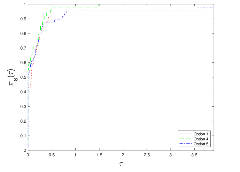
Figure 1. Performance profile comparing function evaluations using MSS with three different initializations and $m=3$.

Table 2 presents the cumulative results for $m=3$ for all five initializations. In this table, the total number of function evaluations reported includes only the 46 problems on which the MSS method converged using all five initializations. Table 2 shows that Option 4 appears to outperform the other initializations in number of problems MSS could solve but also in terms of the total number of function evaluations when considering only the problems in which all initializations led to convergence for MSS.

Table 2. Cumulative results on 49 CUTEst problems for $m=3$.

	Option 1	Option 2	Option 3	Option 4	Option 5
Problems solved	47	48	48	49	48
Function evaluations (FE)	8295	7570	9255	6809	6944

Finally, for comparison between the different memory allocations, we report in Table 3 the performance of Option 4 using all three memory size $m=3,5,$ and $7$. The number of function evaluations found in Table 3 for $m=3$ are different than in Table 2 since Table 2 reports results only on 46 problems; in contrast, function evaluations for all 49 problems are included in Table 3 since using MSS converged on all 49 problems for all three memory sizes using Option 4.

Table 3. Cumulative results on 49 CUTEst problems using MSS with Option 4.

memory	$m=3$	$m=5$	$m=7$
Problems solved	49	49	49
Function evaluations (FE)	12,457	14,613	15,232

Experiment 2. One of the most-used indefinite updates for large-scale optimization is the limited-memory symmetric rank-one (L-SR1). For this experiment, we implemented a standard L-SR1 trust-region method [9, Algorithm 6.2] and chose the approximate solution to the subproblem using a truncated-CG (see, for example, [9, 10]). The LSR-1 method was initialized using $B_{0}=\gamma^{SR1}_{k}I$, where $\gamma^{SR1}_{k}$ could be changed each iteration. Updates to the quasi-Newton pairs were accepted provided

$$|s_{k}^{T}(y_{k}-B_{k}s_{k})|\geq\tau_{s}\|y_{k}-B_{k}s_{k}\|\|s_{k}\|,$$ (28)

where $\tau_{s}=1e^{-8}$. For these experiments, the initial iteration used $B_{0}=I$, and for subsequent iterations, the LSR-1 method was initialized two standard ways: (1) using the BB initialization and (2) using $B_{0}=I$ for every initialization. Since we require (28) to update the pairs, there was no danger of the denominator for the BB initialization becoming zero. For these results, the trust-region framework (e.g., parameters) for the MSS and L-SR1 methods were identical. The results of this experiment are presented in a performance profile and table.

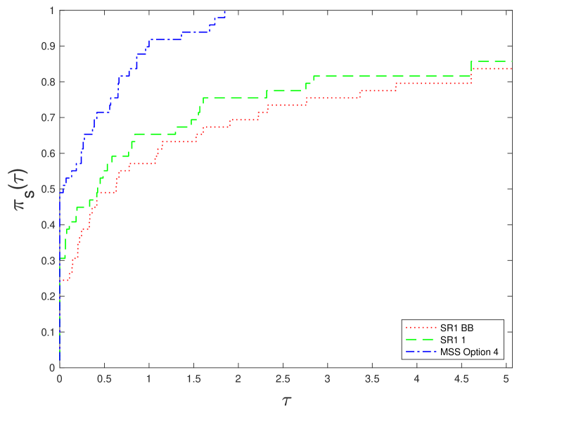
Figure 2. Performance profile comparing function evaluations using L-SR1 and MSS with $m=3$. ”SR1 BB” refers to using L-SR1 together with the BB initialization and ”SR1 1” refers to using L-SR1 together with the initialization $B_{0}=I$ each iteration.

Figure 2 contains the performance profile for function evaluations. From the figure, it appears that MSS with Option 4 outperforms both implementations of L-SR1 in terms of function evaluations using $m=3$. Table 4 contains cumulative results for $m=3$ for MSS and the two L-SR1 methods. Of the 49 problems that at least one method converged on, MSS converged on all 49; meanwhile, the L-SR1 methods converged on 41 and 42 depending on the initialization. There were a total of 40 problems in which all three method converged; the total number of function evaluations on these 40 problems are reported in the last line of table. On the problems in which all three methods converged, MSS required significantly fewer function evaluations. In table 5, the number of problems solved and the number of function evaluations are reported for memory sizes $m=3$, $m=5$ and $m=7$. In all cases, MSS outperformed L-SR1. Note that the total number of function evaluations only counts the 38 problems on which all methods converged using all three memory sizes.

Table 4. Cumulative results on 49 CUTEst problems using MSS with Option 4 and L-SR1.

	MSS	L-SR1 BB	L-SR1 1
Problems solved	49	41	42
Function evaluations (FE)	3,120	14,621	11,817

Table 5. Cumulative results on 49 CUTEst problems using MSS with Option 4 and L-SR1 for various memory sizes.

Memory	Solver	Problems solved	Function evaluations (FE)
	MSS Option 4	49	2,914
$m=3$	L-SR1 BB	41	14,142
	L-SR1 1	42	11,643
	MSS Option 4	49	3,069
$m=5$	L-SR1 BB	40	12,823
	L-SR1 1	44	12,928
	MSS Option 4	49	3,005
$m=7$	L-SR1 BB	41	13,200
	L-SR1 1	43	11,660

Figure 3 contains the performance profile for total time needed to solve each problem for the case $m=3$. From the profile, MSS with Option 4 takes significantly less time than either L-SR1 method. For the cases $m=5$ and $m=7$, the results are similar.

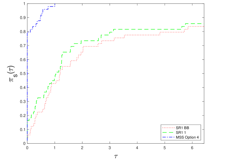
Figure 3. Performance profile comparing runtime using L-SR1 and MSS with $m=3$. ”SR1 BB” refers to using L-SR1 together with the BB initialization and ”SR1 1” refers to using L-SR1 together with the initialization $B_{0}=I$ each iteration.

Experiment 3. In this section, we compare the MSS method with a dense initialization to the limited-memory Powell-symmetric-Brodyen (PSB) method. Similar to the MSS update, the PSB update is a rank-2 quasi-Newton update that can generate indefinite Hessian approximations; thus, it is natural to use both methods in a trust-region framework. Moreover, PSB admits a compact representation [23] enabling us to use the same OBS-like solver that used for MSS. In other words, to use PSB, the only changes in Algorithm 1 for MSS that need to be made to use PSB are (i) the definition of $M$, (ii) the definition of $\Psi$, and (iii) the removal of the requirement that $S$ is full rank in line 18. (For more details on the PSB update, see, e.g., [23].) For these experiments, a limited-memory PSB method was initialized using (i) $B_{0}=\gamma_{k}I$, where $\gamma_{k}=(y_{k}^{T}y_{k})/(s_{k}^{T}y_{k})$ (i..e, the BB initialization) and (ii) $B_{0}=\gamma_{k}I$, where $\gamma_{k}=(s_{k}^{T}y_{k})/(s_{k}^{T}s_{k})$, which is denoted as the ”oBB” initialization in the table. Note that both these initialization are inspired by the results of (Theorem 3) with the stored vectors limited to the most current quasi-Newton pair (i.e., the number of stored pairs is one).

Figure 4–6 contains the performance profile for function evaluations. From the figure, it appears that MSS with Option 4 outperforms both implementations of L-PSB in terms of function evaluations using $m=3$, $m=5$, and $m=7$, respectively. Table 6 lists cumulative results for these different memory sizes and initializations. To compute the total number of function evaluations in the table, only the problems on which all three methods using all three memory sizes were considered–this amounted to 45 problems. From the table, MSSM performs best on this test set for smaller memory sizes; in contrast, L-PSB with the BB initialization solved more problems with smaller memory sizes but the total number of function evaluations on the 45 problems was smallest with $m=5$. Meanwhile, L-PSB with the oBB initialization performed better with larger memory sizes.

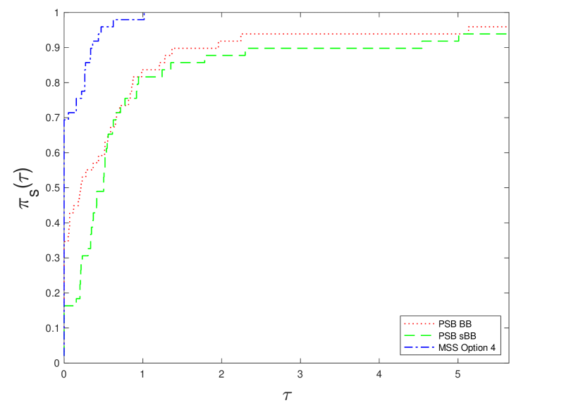
Figure 4. Performance profile comparing function evaluations using L-PSB and MSS with $m=3$. ”PSB BB” refers to using L-PSB together with the BB initialization and ”PSB sBB” refers to using L-PSB together with the initialization $B_{0}=(s_{k}^{T}y_{k})/(s_{k}^{T}s_{k})I$ each iteration.

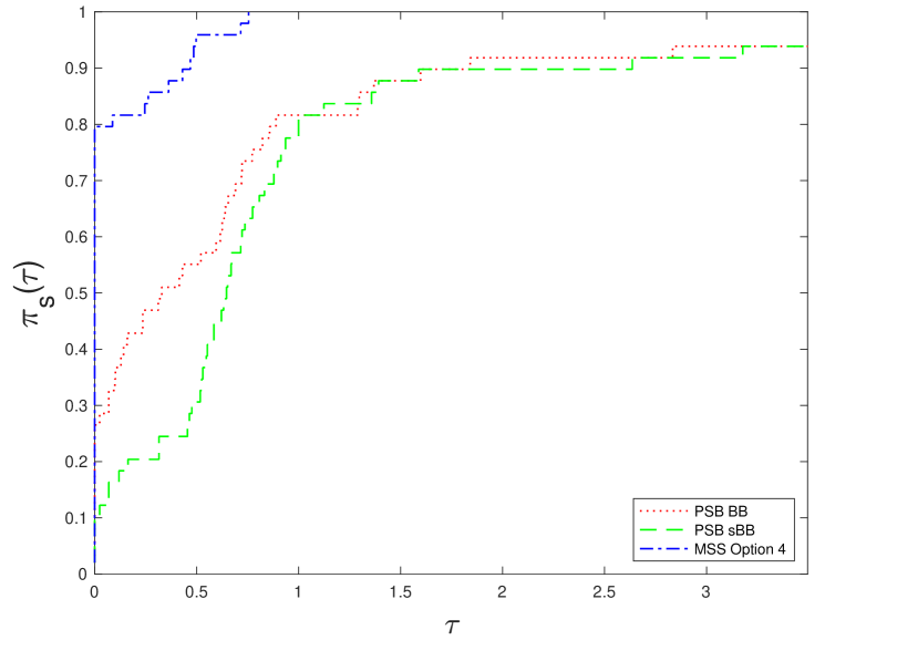
Figure 5. Performance profile comparing function evaluations using L-PSB and MSS with $m=5$. ”PSB BB” refers to using L-PSB together with the BB initialization and ”PSB sBB” refers to using L-PSB together with the initialization $B_{0}=(s_{k}^{T}y_{k})/(s_{k}^{T}s_{k})I$ each iteration.

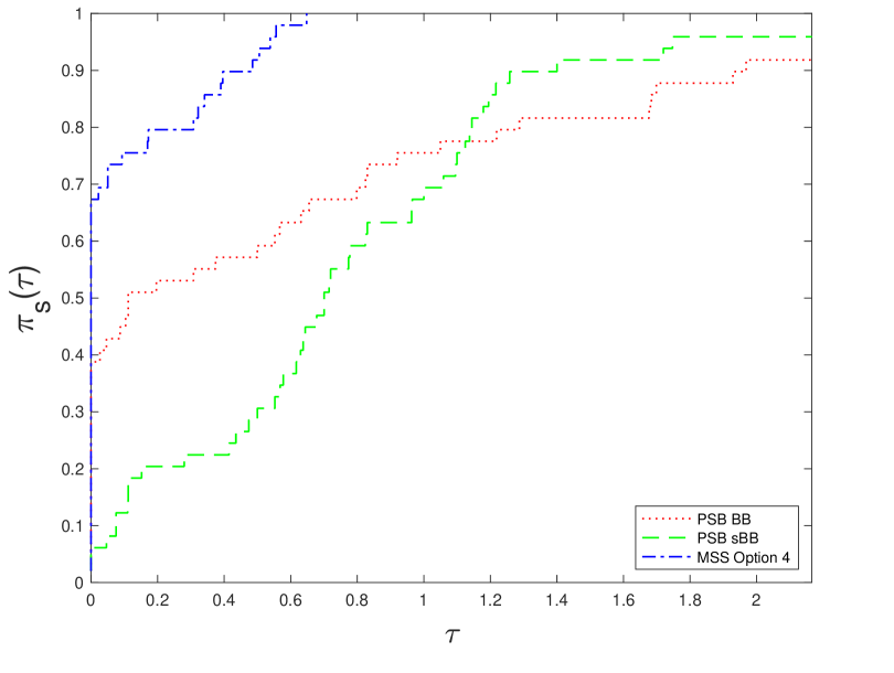
Figure 6. Performance profile comparing function evaluations using L-PSB and MSS with $m=7$. Here, ”PSB BB” refers to using L-PSB together with the BB initialization and ”PSB sBB” refers to using L-PSB together with the initialization $B_{0}=(s_{k}^{T}y_{k})/(s_{k}^{T}s_{k})I$.

Table 6. Cumulative results on 49 CUTEst problems using MSS with Option 4 and L-PSB for various memory sizes. Here, ”PSB BB” refers to using L-PSB together with the BB initialization and ”PSB sBB” refers to using L-PSB together with the initialization $B_{0}=(s_{k}^{T}y_{k})/(s_{k}^{T}s_{k})I$.

Memory	Solver	Problems solved	Function evaluations (FE)
	MSS Option 4	49	5927
$m=3$	L-PSB BB	47	11,336
	L-PSB oBB	46	14.529
	MSS Option 4	49	6,290
$m=5$	L-PSB BB	46	11,157
	L-PSB oBB	46	10,705
	MSS Option 4	49	6,648
$m=7$	L-PSB BB	45	12,951
	L-PSB oBB	47	10,694

Finally, the performance profile for total runtime on the test set of 49 problems with $m=3$ for MSS with Option 4 and the two PSB methods are found in Figure 7. This figure shows that MSS with Option 4 was the faster of the three methods on this test set.

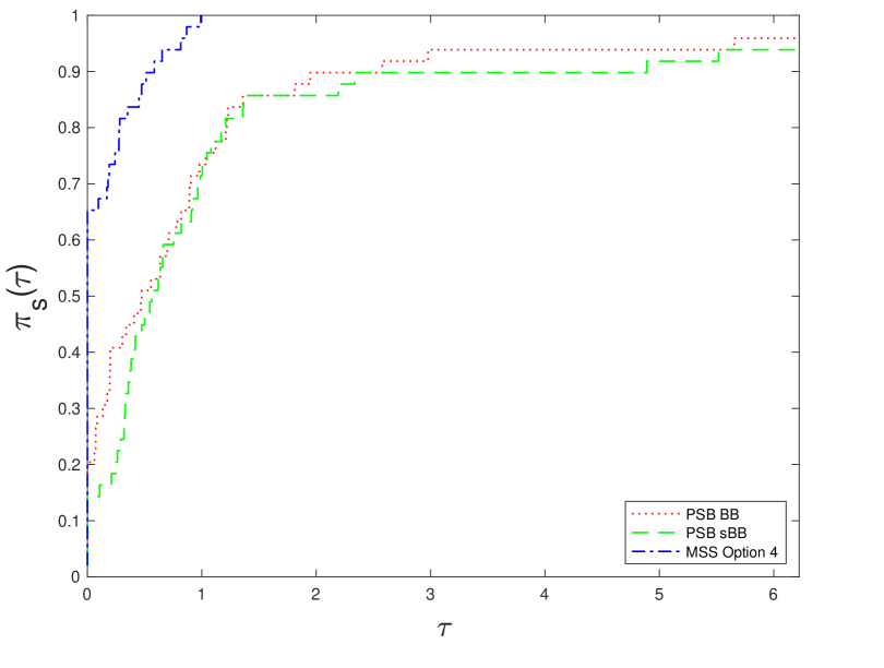
Figure 7. Performance profile runtime using L-PSB and MSS with $m=3$. Here, ”PSB BB” refers to using L-PSB together with the BB initialization and ”PSB sBB” refers to using L-PSB together with the initialization $B_{0}=(s_{k}^{T}y_{k})/(s_{k}^{T}s_{k})I$.

6. Concluding Remarks

In this paper, we demonstrated how a dense initialization can be used with a MSS method. In numerical experiments on CUTEst test problems, the dense initialization performs better than standard constant diagonal initializations. Results suggest that this method performs well with small memory sizes (i.e., $m=3$ outperformed the other memory sizes and the number of function evaluations generally increased as $m$ increased). Moreover, with small $m$, the proposed method generally outperforms a basic L-SR1 trust-region method. Further research includes considering other symmetrization, choices for the two parameters $\zeta$ and $\zeta^{C}$, and trust-region norms (including the so-called shape-changing norm first proposed in [24]). The results of future research will be submitted in subsequent papers.

6.1. Acknowledgement.

The authors would like to thank the referees. In particular, one referee provided an explanation that led to the inclusion of Lemma 3 and significantly improved the entire section. In fact, part of the proof is based on an observation by the referee.

Funding

J. B. Erway’s research work was funded by NSF Grant IIS-1741264.

References

- [1] Oleg P Burdakov. Methods of the secant type for systems of equations with symmetric jacobian matrix. Numerical functional analysis and optimization, 6(2):183–195, 1983.
- [2] Oleg P Burdakov, José Mario Martínez, and Elvio A Pilotta. A limited-memory multipoint symmetric secant method for bound constrained optimization. Annals of Operations Research, 117(1-4):51–70, 2002.
- [3] Robert B Schnabel. Quasi-newton methods using multiple secant equations. Technical report, Colorado University at Boulder Department of Computer Science, 1983.
- [4] Johannes Brust, Oleg Burdakov, Jennifer B. Erway, and Roummel F. Marcia. A dense initialization for limited-memory quasi-Newton methods. Computational Optimization and Applications, 74(1):121–142, 2019.
- [5] Nicholas I. M. Gould, Dominique Orban, and Philippe L. Toint. Cutest: a constrained and unconstrained testing environment with safe threads for mathematical optimization. Computational Optimization and Applications, 60(3):545–557, 2015.
- [6] Johannes Joachim Brust. Large-Scale Quasi-Newton Trust-Region Methods: High-Accuracy Solvers, Dense Initializations, and Extensions. PhD thesis, UC Merced, 2018.
- [7] J. E. Dennis, Jr. and Jorge J. Moré. Quasi-newton methods, motivation and theory. SIAM Review, 19(1):46–89, 1977.
- [8] Richard H. Byrd, Jorge Nocedal, and Robert B. Schnabel. Representations of quasi-newton matrices and their use in limited memory methods. Mathematical Programming, 63(1):129–156, 1994.
- [9] Jorge Nocedal and Stephen Wright. Numerical optimization. Springer Science & Business Media, 2006.
- [10] Andrew R Conn, Nicholas IM Gould, and Philippe L Toint. Trust region methods. SIAM, 2000.
- [11] David M Gay. Computing optimal locally constrained steps. SIAM Journal on Scientific and Statistical Computing, 2(2):186–197, 1981.
- [12] Jorge J Moré and Danny C Sorensen. Computing a trust region step. SIAM Journal on Scientific and Statistical Computing, 4(3):553–572, 1983.
- [13] Jennifer B. Erway and Roummel F. Marcia. Algorithm 943: MSS: Matlab software for l-bfgs trust-region subproblems for large-scale optimization. ACM Trans. Math. Softw., 40(4), 2014.
- [14] Oleg Burdakov, Lujin Gong, Spartak Zikrin, and Ya-xiang Yuan. On efficiently combining limited-memory and trust-region techniques. Mathematical Programming Computation, 9(1):101–134, 2017.
- [15] Johannes Brust, Jennifer B Erway, and Roummel F Marcia. On solving L-SR1 trust-region subproblems. Computational Optimization and Applications, 66(2):245–266, 2017.
- [16] Jennifer B Erway and Roummel F Marcia. On efficiently computing the eigenvalues of limited-memory quasi-Newton matrices. SIAM Journal on Matrix Analysis and Applications, 36:1338–1359, 2015.
- [17] Jonathan Barzilai and Jonathan M. Borwein. Two-point step size gradient methods. IMA Journal of Numerical Analysis, 8(1):141–148, 01 1988.
- [18] Johannes Brust, Oleg Burdakov, Jennifer Erway, and Roummel Marcia. Algorithm xxx: SC-SR1: MATLAB software for solving shape-changing L-SR1 trust-region subproblems. Technical report, arXiv:1607.03533 [math.OC], 2021.
- [19] Desmond J. Higham and Nicholas J. Higham. MATLAB Guide. SIAM, third edition, 2017.
- [20] Nicholas J. Higham. Accuracy and Stability of Numerical Algorithms. SIAM, 2nd edition, 2002.
- [21] Jorge Nocedal. Updating quasi-newton matrices with limited storage. Mathematics of Computation, 35(151):773–782, 1980.
- [22] Elizabeth D. Dolan and Jorge J. Moré. Benchmarking optimization software with performance profiles. Mathematical Programming, 91:201–213, 2002.
- [23] Michael J.D. Powell. A new algorithm for unconstrained optimization. In J.B. Rosen, O.L. Mangasarian, and K. Ritter, editors, Nonlinear Programming, pages 31–65. Academic Press, 1970.
- [24] Oleg Burdakov and Ya-xiang Yuan. On limited-memory methods with shape changing trust region. In Proceedings of the First International Conference on Optimization Methods and Software, page p. 21, 2002.