What do writing features tell us about AI papers?

Abstract

As the numbers of submissions to conferences grow quickly, the task of assessing the quality of academic papers automatically, convincingly, and with high accuracy attracts increasing attention. We argue that studying interpretable dimensions of these submissions could lead to scalable solutions. We extract a collection of writing features, and construct a suite of prediction tasks to assess the usefulness of these features in predicting citation counts and the publication of AI-related papers. Depending on the venues, the writing features can predict the conference vs. workshop appearance with F1 scores up to 60-90, sometimes even outperforming the content-based tf-idf features and RoBERTa. We show that the features describe writing style more than content. To further understand the results, we estimate the causal impact of the most indicative features. Our analysis on writing features provides a perspective to assessing and refining the writing of academic articles at scale.

1 Introduction

As technology continues to develop rapidly, conferences and journals have increased numbers of article submissions. There is increased criticism from multiple sides. On one side, authors criticize the randomness and subjectivity of peer reviews (Rogers and Augenstein, 2020; Church, 2020). On the other side, reviewers worry about the quality of papers, frequently raise concerns, and reject most submissions.

The tension reveals an underlying problem: it is hard to assess the quality of academic articles (1) automatically, (2) with high accuracy, and (3) in a way that is convincing to humans. An ideal evaluation system should meet all three criteria. Unfortunately, current systems can satisfy at most two of the three.

• Human-based peer reviewing is the de-facto system. Thanks to the detailed reviewer comments, this system gives the most convincing results. While some components (e.g., paper - reviewer matching) can be automated, this system is largely run by humans.

• Automatic essay scoring (AES) systems are automatic, but they are developed and applied in the domain of student essay scoring, a completely different domain from scholarly articles. Transferring between domains limits the possible accuracy.

• Deep neural network systems can automatically predict paper appearance with reasonable accuracy, but the granularities of their results are coarse, compared to feature-based AES systems.

Is that possible to build scalable systems that reach all three criteria simultaneously, to assist the human reviewers? In this paper, we argue that studying the interpretable properties of articles could lead to potential solutions.

Academic articles, despite some structural guidance or precedent, are fundamentally a form of discourse, where many features have been shown to have perlocutionary effects. For example, shorter sentences, and the use of certain rhetorical devices (e.g., amplification) can attract the readers’ attention, and could boost the popularity of social media posts (Page, 2013). These devices are especially popular among political discourse, and are also used widely (Janks, 1997; Browse, 2018; Catalano and Waugh, 2020).

Looking from a discourse analysis perspective, a series of questions quickly emerge. Can the factors related to discourse, rather than the contents of an article, impact where the papers appear? If an article is written with shorter sentences, or written in more readable forms, will future researchers be more inclined to cite it? The query from these questions motivates us to study writing features.

We compute a collection of writing features describing distinct discourse aspects of an article (e.g., the proportion of active voice in abstract), that are independent of content or topic (§3). We construct a suite of prediction tasks using a dataset containing 945,674 published computer science papers (§4). We find that the annual citation counts are hard to predict (§5.1). However, the conference vs. workshop appearance of some top-tier venues can be predicted using writing features with F1 scores up to 60-90, sometimes even outperforming the content-based classifiers (§5.2). With inter-venue and inter-category classification tasks, we illustrate that the writing features describe the styles instead of the contents (§5.3). To further understand the results, we estimate the causal impacts of the most indicative features and study their empirical indications to paper publications (§5.4).

We release the writing features and the test suite. Our work presents a new perspective towards building scalable and interpretable systems for assessing and refining academic articles.

2 Related Work

Reflections on Peer Review

Researchers have discussed how the peer review process could be improved (Kelly et al., 2014; De Silva and K. Vance, 2017). Recently, the peer review process has been called into doubt (Stelmakh et al., 2019; Church, 2020). Bharadhwaj et al. (2020) found that the presence on arXiv affects the acceptance decisions of ICLR papers, especially the borderline ones. These reflections on peer review show the difficulty to assess the qualities of academic articles automatically, convincingly, and with high accuracy.

Automatic Essay Scoring

A survey by Ke and Ng (2019) grouped features most used by state-of-the-art AES systems into ten categories: length, lexical, embedding, category-based, prompt-relevant, readability, syntactic, argumentation, semantics, and discourse. Each AES system used several of them. Some previous AES approaches also included deep learning (Wang et al., 2018a; Dong and Zhang, 2016) but, in this paper, we follow the feature engineering route. We expand this discussion in §3.

Acceptance and citation link prediction

Previous work automatically predicted the acceptance of academic papers using the gestalt (Huang, 2018), or the texts (Yang et al., 2018; Li et al., 2020). Wang et al. (2021) predicted acceptance at the institutional level. There are also methods to predict citation counts, using either engineered features (Yan et al., 2011) or BERT-based models van Dongen et al. (2020). In this paper, we include the citation link prediction and the venue appearance (instead of acceptance, since most rejected papers are not publicly viewable) tasks in our evaluation suite.

Causal analysis with text features

Causal reasoning on text features allows us to estimate the effects of the factors that are encoded in the texts (Kang et al., 2017; Wood-Doughty et al., 2018; Egami et al., 2018), and to measure classifier performance attributable to textual attributes (Pryzant et al., 2018a) and lexicons (Pryzant et al., 2018b). Recent works use causal reasoning to explain the model performance (Feder et al., 2019), and to reveal confoundings (Vig et al., 2020; Keith et al., 2020). Fytas et al. (2021) looks for interpretable factors contributing to paper acceptance. Vincent-Lamarre and Larivière (2021) studies the impact of some discourse features to AI paper acceptance. We use a simple model to estimate the causal effects of distinct writing features towards venue appearance (§5.4).

3 Extracting Writing Features

We consider features depicting the quality of writing in an article, as in AES systems (Ke and Ng, 2019), while avoiding content to the extent possible. Except for those defined on the whole article (e.g., title length), we compute each feature on the abstract and the bodytext respectively.

Citation counts features (1 label, 0 feature)

• The annual inbound citations reflect the value of the articles, as perceived by other authors (Hou and Ma, 2020). Each article may receive a different number of inbound citations each year, but we count the normalized number and refer to them as the annual citation counts henceforth.

• The total inbound citation counts. This is highly correlated to annual citation counts ($R=0.9472$, while the remaining features have at most $R=0.3$). The articles with high academic merit would be cited more annually and would have more accumulative citations, so we consider the total inbound citation count “synonymous” to the annual citations. Since we already have the annual counts, we exclude the total counts from the regression and classification experiments.

Article-metadata (3 features)

• Title length, measured in the number of words. There are slight negative correlations between the title length and the total citations of articles (Letchford et al., 2015), but that can be explained by the scope of the content. The papers with shorter titles discuss more general topics, therefore may reach larger audiences.

• Number of authors.

• The outbound citations per word. This is the number of previous articles that the article that we analyze cite, normalized by the word counts. A more general article or a literature review tends to contain more outbound citations per word.

Article length (5 features)

These include the number of sections, the number of words and sentences in the abstract and body text. In subsequent analysis using 85 features, we include all 5. For those using 74 features (i.e., removing the effects of body text length), we include 2: the number of words and sentences in the abstract. Note that some features in other categories are also relevant to article length. For example, the number of grammatical errors in the body text, and the total number of outbound citations.

Sentence length (4 features)

The lengths of sentences are relevant to readability. Longer sentences are in general harder to read through, but strategic use of long and short sentences could contribute to the styles of writings (Strunk, 2007). This category includes the mean and variance of lengths of each sentence. They are computed for the abstract and the bodytext respectively. Unless specified, each subsequent feature is likewise computed.

Flesch Readability (4 features)

We use two scores, the Flesch readability ease (RE) (Flesch, 1948) and the Flesch-Kincaid grade level (GL) (Kincaid et al., 1975), to describe the ease of reading. The scores are computed as follows.

RE $$=206.835-1.015\frac{W}{L}-84.6\frac{S}{W}$$

GL $$=0.39\frac{W}{L}+11.8\frac{S}{W}-15.59,$$

where $S$, $W$, and $L$ are the syllable, word, and sentence counts, respectively.

Here, a higher syllable/word ratio $\frac{S}{W}$ correlates to the usage of more complex words, and a higher word/sentence ratio $\frac{W}{L}$ signals the use of relatively longer and more sophisticated sentences. Therefore, a higher readability ease (RE) value indicates the article being simpler, while a higher grade level (GL) indicates greater complexity. The RE and GL scores are used to refine the reading material for a potential audience, and assess the cognitive loads imposed by texts (Roberts et al., 2016; Kelly, 2017; Wang et al., 2018b; Fakhoury et al., 2018)

Grammatical error count (2 features)

Grammatical errors have been used as a factor in AES systems to assess, e.g., language learners’ writing abilities (Attali and Burstein, 2006; Shermis and Burstein, 2003). We use a state-of-the-art grammar error correction model, open-sourced by Grammarly, GECToR (Omelianchuk et al., 2020). GECToR is a RoBERTa-based neural model which corrects the grammatical mistakes in a sequence tagging. We compute the number of “grammar mistake” tags recommended by GECToR in both the abstracts and the bodytexts, for each article.

Lexical richness (10 features)

Lexical richness has been used to analyze writing style (Smith and Kelly, 2002), vocabulary, and writing skills (Laufer and Nation, 1995; Gregori-Signes and Clavel-Arroitia, 2015). There are many methods (“indices”) to describe lexical richness (Malvern and Richards, 2012). In this paper, we use a method that is invariant to the article length: the moving-average type-token ratio (MATTR, Covington and McFall (2010)). A higher MATTR value indicates a less repetitive usage of words.

To compute MATTR: First compute the type-token ratio (TTR):

$$\text{TTR}=\frac{N.\text{types}}{N.\text{tokens}},$$

where the number of types is the number of distinct tokens. Then average over some fixed length windows (we use 5, 10, 20, 30, 40) to get the MATTR with 5 different window lengths. We use a Python library to compute MATTR on the abstract and the bodytext of each article.

Part-of-speech constituency (28 features)

We compute the part-of-speech constituency. We use the 14 PoS tags (in English) given by SpaCy The tags are: ADJ, ADV, ADP, AUX, CCONJ, DET, INTJ, NOUN, NUM, PART, PRON, PROPN, SPACE, VERB. The constituency of e.g., NOUN in abstract is computed by the percentange of occurrence of the NOUN tag in the abstract of an article. Various researchers consider part-of-speech to be an important signal related to the syntactical information encoded in the text (Jurafsky and Martin, 2000; Zeman et al., 2019; Tenney et al., 2019). The choice of part-of-speech has been used as a marker for writing style (Campbell and Pennebaker, 2003), language fluency for foreign language learners (Alderson, 2005), and even cognitive capacity (Fraser et al., 2015).

Sentential surprisal (4 features)

This is computed by the average log perplexity of GPT-2 – a pretrained uni-directional language model (Radford et al., 2019) – when reading through the first token of each sentence in an article. For an article consisting of $N$ sentences $\{s_{1},...,s_{N}\}$, the sentential surprisal is computed as:

$$\text{SS}=\mathbb{E}_{i}\text{ log}P(s_{i+1}^{(0)}\,|\,s_{1..i}),$$

where $s_{i}^{(j)}$ refers to the $j^{th}$ token in the $i^{th}$ sentence of the article.

We can interpret the sentential surprisal scores as follows. If there are large “semantic gaps” from sentence to sentence, then the overall difficulty for comprehension is increased, and a unidirectional language model will show higher perplexity. Table 1 presents two examples. Note that other factors can impact the perplexity values produced by the language models, including the word frequency and the choice of grammar. Note that both the word frequency (Shain, 2019) and the grammatical forms (Gough, 1965) are relevant to the ease of understanding the text. Regardless, the “semantic gaps” are not necessarily causative to the sentential surprisal scores of the language models, but they are correlative (Goodkind and Bicknell, 2018).

Sentences	Surprisal
We propose a network based on BERT. We describe the network as following.	90.194
We propose a network based on BERT. Recently, deep neural networks are widely used.	92.861

Table 1: Two examples of sentences. The surprisal values are the log probability of the underlined tokens, as computed by a pretrained GPT-2 (Radford et al., 2019). The former example follows a more natural flow of writing. In the second example, the background is written after the detailed activity on purpose, and it has a larger surprisal value.

Rhetorical signal constituency (18 features)

Academic papers, like other types of articles written with specific goals, contain many rhetorical devices. We use Rhetorical Structure Theory (RST) (Mann and Thompson, 1987) to quantitatively describe the rhetorical activities in the articles.

Recently, RST features have been used in developing some AES systems (Wang et al., 2019). They are related to both the style and content of articles. For example, a theoretical article presenting an abstract idea may contain extensive elaboration and explanation signals, while a perspective article written to contribute to a debate likely contains more contrast and comparison signals.

We parse the abstracts of the articles with a pretrained RST parser (Feng and Hirst, 2014), and count the proportion of each RST signal. Note that we only consider the abstracts due to time constraints. Building an RST parse tree for an abstract takes between 2 to 10 seconds. For a full article, this could take at least 5 minutes. Computing only the $\approx 10^{6}$ articles in the Computer Science category of S2ORC (Lo et al., 2020) would take at least 9 years of computation on available machines, which is unrealistic.

Active and passive voice proportions (6 features)

We count the proportions of active- and passive-voice sentences in both the abstract and the body text. To detect the voice of a sentence, we check the dependency tags of all of its tokens. If the sentence is in the active voice, its subject has a nsubj tag. If it is in passive voice, its nominal subject has a nsubjpass tag. If neither tag occurs in any token of the sentence, we label the sentence as in the “Other” voice. Table 2 shows some examples.

Sentence	Label
We show that dropout improves the performance of neural networks on supervised learning tasks…	Active
In the simplest case, each unit is retained with a fixed probability p independent of…	Passive
Applying dropout to a neural network amounts to sampling a “thinned” network from it.	Other

Table 2: Several example sentences in different voices, taken from a highly cited paper (Srivastava et al., 2014). The underlined words in the active and the passive voice sentence are tagged with the nsubj and nsubjpass dependency tags respectively.

Venue Name	Writing Features						TF-IDF		RoBERTa
	74 features	RST	Surprisal	Grammar	LexRich	Readability	Full text	Abstract	Abstract
AAAI	$.755(.028)$	$+.001$	$+.024$	$+.010$	$-.002$	$+.009$	$+.206^{**}$	$+.203^{**}$	$+.212^{**}$
ACL	$.867(.004)$	$+.001$	$+.000$	$+.001$	$+.001$	$+.001$	$-.004$	$-.008^{*}$	$-.015$
COLING	$.837(.010)$	$+.005$	$+.005$	$+.003$	$+.003$	$+.004$	$+.049^{**}$	$+.051^{**}$	$+.052^{**}$
CVPR	$.900(.005)$	$-.007$	$-.006$	$-.001$	$-.006$	$-.005$	$-.052^{**}$	$-.067^{**}$	$-.070^{**}$
EMNLP	$.737(.020)$	$+.003$	$+.014$	$+.012$	$+.022$	$+.015$	$+.159^{**}$	$+.153^{**}$	$+.102$
ICML	$.659(.023)$	$-.277^{**}$	$-.042^{*}$	$-.102$	$-.262^{**}$	$-.185$	$+.333^{**}$	$+.333^{**}$	$+.300^{**}$
IJCAI	$.868(.002)$	$-.067^{**}$	$-.066^{**}$	$-.045^{**}$	$+.075^{**}$	$-.067^{**}$	$-.029^{**}$	$-.061^{**}$	$-.076$
NAACL	$.757(.019)$	$+.016$	$+.016$	$+.011$	$+.017^{*}$	$+.016^{*}$	$-.107^{**}$	$-.128^{**}$	$-.182$
NeurIPS	$.586(.035)$	$-.193^{**}$	$-.039$	$-.097$	$-.212^{**}$	$-.157$	$+.031$	$-.077^{*}$	$-.110$

Table 3: F1 scores of the C vs. W classification results. The second column shows the mean and stdev of F1 scores using 74 writing features. The remaining columns show the values relative to the second column. $*$ and $**$ indicate $p<.005$ and $p<.001$ respectively, both on 2-tailed $t$-test with $dof=10$, Bonferroni corrected.
Interpretation: Usually, writing features do not classify as well as the content-based classifiers, but sometimes the difference is not significant (e.g., ACL). In CVPR and NAACL, writing features are even better.

4 Data

We use the Semantic Scholar Open Research Corpus (S2ORC) (Lo et al., 2020). S2ORC is currently the largest publicly available collection of research articles, approximately 320 times larger than the ACL Anthology dataset (Radev et al., 2009).

There are 19 subjects in S2ORC. We use the Computer Science category, containing 4,305,658 articles. Among them, 994,434 articles contain full texts. We computed the features mentioned in section 3 and removed nan entries, resulting in 945,674 articles.

Citation profile

Among these articles, 923,699 ($97.68\%$) have $\leq 10$ annual incoming citations. 937,381 ($99.12\%$) have less than $\leq 20$ annual incoming citations. For simplicity, we use the term “citation” to refer to incoming citations (i.e., how many times an article is cited), and do not abbreviate the outbound citation counts (i.e., how many times it cites others) in the rest of this article. On average, each article is cited $1.59$ (std=$13.5$) times per year. As shown in Figure 4 (in Appendix), the number of articles decreases exponentially as the annual citation counts increase.

Article categories

The S2ORC dataset provides noisy labeling of the venue and journal occurrences for each article. For simplicity, we refer to “venue or journal” as “venue”. We filter some venue names in various categories with keyword-based regex matching. In NLP, ML, AI, and CV, there are $6,681$ venues/journals containing about 465k CompSci articles. Table 5 (in Appendix) shows the details.

Venue labels

Additionally, we mark each venue of our selected categories with a binary C or W label. In general, a C label stands for top-tier conferences, where a W label stands for workshops and general arXiv papers. That said, workshops with high impacts (as shown in the Google Scholar Metrics and guide2research), including SemEval, *SEM, and Rep4NLP, are labeled as C as well. Table 6 (in Appendix) contains some examples of labeling. Table 7 shows the numbers of articles in each venue. Specifically, we consider 9 top-tier venues:

• NLP: ACL, NAACL, EMNLP, COLING

• Machine learning: NeurIPS, ICML

• Artificial intelligence: AAAI, IJCAI

• Computer vision: CVPR

These 9 venues (including their workshops) contain 12,747 articles. Among the top-tier papers, the mean annual citation count is $7.28$ (std=$67.8$). Their citation profile also obeys a exponential distribution (Figure 4 in Appendix).

((a)) With all writing features.

((b)) With tf-idf features.

Figure 1: The AUROC of inter-venue classifications. The venues in the same categories (e.g., COLING and ACL) are harder to tell apart than other venues, using either the writing features or tf-idf features.

((a)) With all writing features.

((b)) With tf-idf features.

Figure 2: The AUROC of inter-category classifications. The content-based tf-idf features can better predict the categories of the articles than the writing features ($p<.01$ for all categories, 2-tailed $t$ test with $dof=8$).

5 Experiments

5.1 Citation counts are hard to predict

The annual citation counts is perhaps the most objective quantity related to the impact of articles. It turns out that the current writing features, no matter when using together or in most combinations, cannot predict annual citation counts better than a trivial baseline (the mean annual citation counts of training data). The annual citation counts seem more relevant to the contents, instead of the writing styles. The content-based features (i.e., tf-idf) produce MSEs with smaller variances, but they do not significantly outperform the baselines either. We include the detail in Appendix A.2.

5.2 Writing features can predict conference vs. workshop appearance

The conference (C) versus workshop (W) discrepancy is an interesting prediction task because many workshops affiliate with conferences. This way, C and W papers are usually about closely relevant topics but written in different styles (due to e.g., page limit requirements).

We let classifier models predict the C vs W appearance on the venues using the writing features, tf-idf features, and RoBERTa (Liu et al., 2019). The experiment detail is in Appendix A.3.

Table 3 shows our results. In general, writing features do not classify the article appearance as good as the content-based tf-idf features (e.g., in AAAI, COLING, EMNLP), but sometimes the difference is not significant (e.g., ACL, NeurIPS). Specifically, in CVPR and NAACL, using 74 writing features significantly outperforms the tf-idf features. These illustrate the usefulness of the writing features.

Should we use all features or a partial set? Since there is no clear evidence suggesting otherwise, we proceed with the collection of 74 features in subsequent analysis to get broad coverage. As we will elaborate in §5.4, the writing features are mutually dependent, so classifying with a partial set can still get comparable results.

5.3 Writing features describe style more than content

The aforementioned C vs. W classification is an intra-venue prediction task. Within each venue, one can argue that the articles follow certain styles. To examine if the writing features describe these styles, we run pairwise classifications between (1) each pair of conferences and (2) each pair of categories, using writing features and tf-idf features.

The first observation is, venues in the same category are harder to tell apart. As shown in Figure 1, the AUROC scores between e.g., ACL and NAACL are lower than that of e.g., ACL and CVPR. However, even the lowest classification performance is much higher than what we would expect from random guessing (0.50 AUROC). This shows that the styles of ACL COLING papers, while similar, are still slightly different. A potential reason is that ACL and COLING have slightly different tracks, and authors have slightly different preferences when writing ACL vs. COLING papers.

Second, in almost all pairwise classification tests, tf-idf features outperform the writing features. This may result from the vocabulary difference across venues – we don’t usually see words like “discourse” in computer vision papers.

Third, while it is relatively easy to distinguish papers between representative venues, it is harder to tell papers apart across categories using writing features, as illustrated by smaller AUROC scores in Figure 2(a) than Figure 1(a). However, this does not apply to the content-based classifications – the use of words contains sufficient information to distinguish between the categories, as is captured by tf-idf features. We consider this a result of the stylistic diversity: The articles can be written in diverse styles regardless of the category. Both an NLP and an AI paper can be written in short sentences and readable forms, but their contents are different.

Venue	Features	Spearman R	ATE	Interpretation
ACL	flesch_kincaid_grade_level_bodytext	$-0.05$	$+0.05$	Ambiguous
	grammar_errors_abstract	$-0.09^{**}$	$-0.01$	W papers are larger
	surprisal_abstract_std	$-0.01$	$+0.00$	Ambiguous
	title_word_length	$-0.09^{**}$	$-0.01$	W papers are larger
	voice_bodytext_active	$+0.09^{**}$	$+0.15$	C papers are larger
EMNLP	outbound_citations_per_word	$-0.17^{**}$	$+67.6$	Ambiguous
	n_author	$-0.17^{**}$	$-0.05$	W papers are larger
	grammar_errors_abstract	$-0.18^{**}$	$+0.01$	W papers are larger
	n_outbound_citations	$-0.09$	$+0.09$	Ambiguous
	abstract_word_counts	$-0.16^{**}$	$+0.00$	W papers are larger

Table 4: The most important 5 writing features for classifying C vs. W appearance, their Spearman R, and their estimated average treatment effects (ATE), taking ACL and EMNLP as examples. $*$ and $**$ indicate $p<.005$ and $p<.001$ respectively (Bonferroni corrected). For Spearman R, the $p$ value indicates the likelihood the feature and target come from identical distributions. For ATE, the $p$ value is computed by doWhy’s default bootstrapping test.

5.4 Writing features describe interpretable characteristics of venue appearance

Here we attempt to further understand the classification results by studying the top 5 features identified by the best classification models in §5.2. We compute the Spearman correlation (to the appearance) and the Average Treatment Effect (ATE) for each feature.

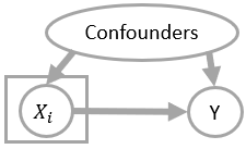
The ATE of a feature $X_{j}$ to the target $Y$ is the expected partial derivative $\frac{\partial\mathbb{E}Y}{\partial X_{j}}$. We estimate the ATE values with doWhy (Sharma et al., 2019)’s “backdoor.linear_regression” algorithm, using a simple causal model. As shown in Figure 3, we assume each of the 74 writing features is causally related to the target while being independent of each other.

Spearman R and ATE provide two aspects of understanding the features independently. If both scores have the same signs, we consider this feature to be indicative of the target. Table 4 shows the indicative features of ACL and EMNLP as examples. The full table (Table 11) is included in Appendix.

grammar_errors_abstract has both negative SpearmanR and ATE values, indicating that C papers are more likely to have fewer grammar errors than W ones. In addition, grammar error counts are identified as a “top-5” feature in AAAI (abstract, 3rd), CVPR (bodytext, 1st), EMNLP (abstract, 3rd), ICML (bodytext, 4th), IJCAI (bodytext, 4th), and NAACL (bodytext, 2nd). It has negative Spearman R values except for CVPR . Reducing the grammar error counts may be beneficial for having a paper appear in top-tier conferences.

Figure 3: A simple causal model for estimating the causal effects of the writing features ($\{X_{j}\}$) towards the paper appearance ($Y=1$ for conference, and $Y=0$ otherwise).

However, not all features have polarities that are as obvious. The flesch_kincaid_ grade_level of bodytext is also identified as a top-5 feature frequently, but its polarity is more ambiguous. Its SpearmanR is negative in AAAI ($-0.08^{*}$) and ACL ($-0.05^{*}$), but positive in NeurIPS ($+0.05$), but in all three scenarios, its ATE estimates take the exact opposite signs. The ambiguous numbers prevent conclusive results about their polarities. In other words, the readability (Flesch-Kincaid grade level) of bodytext does not itself predict conference or venue publications.

Another example is title_word_length. The C papers are correlated to shorter title word lengths (4th in ACL, 1st in COLING), echoing the findings of Letchford et al. (2015). In contrast to their explanation that papers with shorter titles are more readable, our study supports an alternative explanation: that workshop papers are more specialized, leading to their longer titles than the more general conference papers.

Only $22\%$ (10 out of the 45) “top-5 features” have significant estimated causal effects ($p<0.05$ for estimated ATE). This indicates that it is hard to single out a writing feature, manipulate its value (e.g., by modifying the writing style), and facilitate paper publication at a conference. We think the reason is that the writing features are dependent – any stylistic change will affect multiple writing features simultaneously. If an article is written in a more readable style, its sentences are likely shorter, its lexical richness may be smaller, and its part-of-speech constituency may change correspondingly. The inter-dependency of features also explains why using partial collections of features can usually lead to comparable performance as the full set of features (e.g., as shown in Table 3). In the future, our analysis can be extended by e.g., grouping the features into mutually independent feature sets.

6 Discussion

Writing features are more than just writing.

We try to ensure these features reflect the writing, and that they do not explicitly correlate to content – but they might do by hidden confounds. For example, if an article compared its proposed model to many other works in its experiments, its normalized outbound citation count could be large. However, a highly impactful paper, especially one opening up a novel direction, may not need to cite many other papers (e.g., backpropagation (Rumelhart et al., 1985) cites 11 other papers and is cited over 27,000 times). In short, there are various reasons to expect correlation or a lack thereof, the resolution of which we leave to future work.

Good papers are more than well-“written”.

Many highly impactful articles have appeared in workshops before. On one hand, studying the interpretable features inspires us to refine the writing e.g., by reducing the grammatical errors and paying attention to the readability. On the other, we should never ignore the intrinsic, academic quality of articles and their inspirations to future researchers.

Discourse features are text markers.

We can use the writing features in different scenarios, including the debates in online forums, and the interactions during the author response periods (e.g., similar to Gao et al. (2019)). Further, discourse features can be text markers (resembling bio-markers), with which we can quantify and even factor out the undesired impacts to the readers. We can also use interpretable text features to diagnose model predictions, identifying some potential “right for the wrong reason” phenomena (McCoy et al., 2019).

7 Conclusion

In this paper, we study the academic articles through a collection of writing features that describe the interpretable dimensions of their styles without explicitly describing their contents. We compile a suite of prediction tasks to validate the effectiveness of these features. These writing features can predict the conference versus workshop appearance of some top-tier venues, sometimes outperforming the content-based tf-idf features and even RoBERTa. Examining the causal impacts of the indicative features leads to practical discussions about paper quality. Our analysis show a perspective towards automatically assessing and refining the writing of academic articles.

Appendix A Appendices

A.1 Exploratory tables

Category	N. articles	N. articles by label
		C	W
AI	23,642	3,493	20,149
CV	29,881	20,029	9,852
ML	12,628	6,196	6,432
NLP	23,827	14,164	9,663
Robotics	15,634	3,311	12,323
Speech	8,123	6,576	1,547
Others	831,939	–	–

Table 5: Article counts of AI-related papers by category. Note that some venues occur in multiple categories.

Venue	Label	N. articles
ACL	C	2,338
Annual Meeting Of The Association For Computational Linguistics	C	1,434
2019 IEEE/CVF Conference on Computer Vision and Pattern Recognition (CVPR)	C	1,274
Rep4NLP@ACL	C	40
SemEval@NAACL-HLT	C	698
BioNLP@ACL	W	73
WASSA@EMNLP	W	84
AAAI Spring Symposia	W	199
arXiv: Learning	W	298
arXiv: Machine Learning	W	258

Table 6: Examples of venue names and their labels.

Venue Name	N. articles	N. articles by label
		C	W
AAAI	624	395	229
ACL	2,836	2,175	661
COLING	1,860	1,353	507
CVPR	3,495	2,824	671
EMNLP	714	437	277
ICML	930	396	534
ICRA	703	662	41
IJCAI	632	423	209
NAACL	2,142	1,354	788
NeurIPS	930	396	534

Table 7: Number of C and W articles of each venue. The arXiv papers of the corresponding sections are included as W papers. For example, cs.Learning and cs.ML are included in the W portions of ICML and NeurIPS.

Venue Name	Writing Features						Baseline	TF-IDF
	74 features	RST	Surprisal	Grammar	LexRich	Readability		Full text	Abstract
AAAI	$+8.61$	$+0.09$	$+0.69$	$+0.27$	$+1.16$	$+0.61$	$20.77(27)$	$0.07(.02)$	$0.07(.01)$
ACL	$+6.27$	$+0.48$	$+0.11$	$+0.10$	$+0.34$	$+2.89$	$389.76(636)$	$0.15(.01)$	$0.17(.01)$
COLING	$+248.87$	$+3.51$	$+0.05$	$+0.32$	$+0.62$	$+368.18$	$437.76(1006)$	$0.15(.02)$	$0.16(.01)$
CVPR	$-6.11$	$+239.82$	$+9.62$	$+6.90$	$+22.24$	$+12.35$	$15273.45(24710)$	$0.17(.01)$	$0.19(.01)$
EMNLP	$+55211.48$	$+8.12$	$+4.66$	$+42.06$	$+12.11$	$+458.65$	$1194.59(2788)$	$0.15(.02)$	$0.17(.03)$
ICML	$+45.13$	$+6.93$	$+37.59$	$+9.77$	$+988.27$	$+86.97$	$1279.15(1200)$	$0.02(.01)$	$0.02(.02)$
IJCAI	$+8.84$	$+1.37$	$+0.81$	$+1.20$	$+3.77$	$+1.97$	$23.77(25)$	$0.16(.01)$	$0.22(.04)$
NAACL	$+18.04$	$+2.22$	$+0.83$	$+0.99$	$+0.08$	$+195.92$	$420.34(855)$	$0.22(.01)$	$0.22(.01)$
NeurIPS	$+78.25$	$+4.64$	$+6.37$	$+39.81$	$-2.87$	$+76.99$	$3305.99(5216)$	$0.20(.01)$	$0.23(.01)$

Table 8: Mean Squared Errors (MSEs) of the regression results predicting annual citation counts. The “Baseline” and “TF-IDF” columns show the mean and std of MSE. Other columns show MSEs relative to the “Baseline” column. No values are significantly different from the “Baseline” column (partly due to the large variation of the writing features and the baselines), on 2-tailed $t$-test with $dof=10$, Bonferroni corrected. However, the MSEs of tf-idf features have much smaller variances.
Interpretation: The annual citation counts cannot be easily predicted by the writing features. On the other hand, the content-based features can predict annual citation counts with small mean squared errors.

((a)) The histogram plots of annual citations profiles of all CompSci papers.

((b)) The histogram plots of annual citations profiles of the AI-related papers.

Figure 4: The histograms of annual citation profiles. The number of articles decreases exponentially as the annual citation counts increase.

A.2 Regression experiments details

Following are the models used for predicting the annual citation counts in Table 8:

• SVM (LinearSVR) with {L1, L2} loss, and $C=\{0.5,1.0,2.0\}$ regularization.

• LinearRegression, with and without fitting the intercept. When fitting the intercept, with and without normalization.

• ExtraTreesRegressor, with random state 0 and {16, 32, 64, 128} estimators.

• RandomForestRegressor, with random state 0 and {50, 100, 200} estimators.

• Gradient boosting, with random state 0 and maximum depths {2,3,4,5}

• Multiple Layers Perceptrons of various hidden sizes: [10], [20], [40], [80], [10,10], [20,20], and [40,40]

On all 9 venues, running 6 folds of experiments, including sweeping through all above models, takes 2-3 minutes on a desktop machine. The regression on all Computer Science articles (Table 9) uses default MLPRegressor, and takes much longer – around one hour for all folds.

Configuration	MAE (stdev)
All features	2.25 (0.05)
Rank by $|$Spearman R$|$
Top 10 features	1.98 (0.04)
Top 20 features	2.00 (0.03)
Top 40 features	2.16 (0.07)
Article features
Part-of-speech	2.03 (0.04)
Rhetorical features	2.02 (0.06)
Sentential surprisal	2.00 (0.05)
Lexical richness	1.98 (0.03)
Grammar features	1.97 (0.03)
Sentence lengths	1.97 (0.04)
Readability	1.96 (0.03)
Voice ratio features	1.96 (0.04)
Article metadata	1.93 (0.02)*
Article lengths	1.92 (0.08)
Baseline: Mean of train data	1.99 (0.02)

Table 9: Annual citation prediction results on all CompSci papers, using different features. The article-metadata features (title length, num. authors, and num. outbound citations) can predict significantly better than the trivial baseline ($p<.005$ for 2-tailed $t$-test, dof=8, Bonferroni corrected). Other features, while showing some signs of usefulness, are not as predictive.
Interpretation: The annual citation count prediction task requires more information than what is described by writing features.

Venue Name	Writing Features
	All 85 features	All$\backslash$length	74 features	Part-of-speech	Voice
AAAI	$+.010$	$+.013$	$.755(.028)$	$+.014$	$+.008$
ACL	$+.002$	$-.004$	$.867(.004)$	$+.000$	$+.001$
COLING	$-.001$	$+.004$	$.837(.010)$	$+.005$	$+.006$
CVPR	$+.011^{**}$	$-.012$	$.900(.005)$	$-.006$	$-.006$
EMNLP	$+.022$	$-.014$	$.737(.020)$	$+.020$	$+.018$
ICML	$+.006$	$-.013$	$.659(.023)$	$-.195^{*}$	$-.233^{**}$
IJCAI	$-.013$	$+.002$	$.868(.002)$	$-.081^{**}$	$-.067^{**}$
NAACL	$+.008$	$-.001$	$.757(.019)$	$+.017^{*}$	$+.017$
NeurIPS	$-.035$	$-.017$	$.586(.035)$	$-.221^{**}$	$-.178^{**}$

Table 10: C vs W classification using other combinations of writing features. The “74 features” column shows the mean and stdev of F1 scores, and other columns show F1 scores relative to the “74 features” column. $*$ and $**$ indicate $p<.005$ and $p<.001$ respectively (Bonferroni corrected), both on 2-tailed $t-$test with $dof=10$.
Interpretation 1: Dropping the article length features and/or the highly correlated MATTR features almost never make significant difference on the classification performance.
Interpretation 2: The part-of-speech and voice features, like the other feature groups in Table 3, support similar or slightly worse classification performance than the collection of 74 features.

A.3 C vs W classification details

Except from RoBERTa, the classifier models are implemented by scikit-learn (Pedregosa et al., 2011). We run 6-fold cross validation: In each rotation, we use 4,1,1 folds as train, dev, and test data with stratified splitting. We sweep through a collection of models, select the best model on the dev set, and record the F1 score on the test set.

Following are the models used for predicting the C vs W appearance:

• SVM (LinearSVC) with {L1, L2} loss

• Logistic Regressions, with max iteration {100,200} and $C=\{0.5,1.0,2.0\}$ regularization.

• ExtraTreesClassifier, with random state 0 and {16, 32, 64, 128} estimators.

• RandomForestClassifier, with random state 0 and {50, 100, 200} estimators.

• Gradient boosting, with random state 0 and maximum depths {2,3,4,5}

• Multiple Layers Perceptrons of various hidden sizes: [10], [20], [40], [80], [10,10], [20,20], and [40,40]

Considering different venues and the combinations of features, there are $210\times 6$ “classification folds”. In each fold, every model except for MLP produces a “feature importance” score for each feature. When the MLP classifiers have the best performance (this happens in 194 out of 1,260 folds, i.e., $15.4\%$), we skip the feature importance scores. For each of the 210 classification settings, we average the feature importance scores across all folds. This allows us to rank the most important features.

The run time for classifying C vs. W on all venues is around 8 minutes on a desktop with M1 chip, using all writing features. The time is around the same for tf-idf features, which have similar dimensions since we set $d=100$.

A.4 Pairwise classification details

In this section of experiments, we use 74 writing features. For the content-based features, we use tf-idf with 100 dimensions, containing both the abstract and bodytext. In classification of both writing and tf-idf features, we use the default MLPClassifier of scikit-learn (Pedregosa et al., 2011). All classifications here are 5-fold cross validations.

The run time of pairwise classification between the venues is 1.5 minutes for writing features, and 30 minutes for tf-idf. The run time of pairwise classification between the categories of venues is 4 minutes for writing features, and 15 minutes for tf-idf, on a desktop machine.

A.5 Most indicative features for venues

Table 11 includes the most indicative features, their Spearman R and ATE values for all venues.

Venue	Features	Spearman R	ATE	Interpretation
AAAI	n_author	$+0.25^{**}$	$+0.03$	C papers are larger
	sent_lens_bodytext_mean	$-0.16^{**}$	$+0.02$	Ambiguous
	grammar_errors_bodytext	$-0.01$	$-0.02$	W papers are larger
	flesch_kincaid_grade_level_bodytext	$-0.08$	$+0.01$	Ambiguous
	outbound_citations_per_word	$+0.24^{**}$	$+56.06$	C papers are larger
ACL	flesch_kincaid_grade_level_bodytext	$-0.05$	$+0.05$	Ambiguous
	grammar_errors_abstract	$-0.09^{**}$	$-0.01$	W papers are larger
	surprisal_abstract_std	$-0.01$	$+0.00$	Ambiguous
	title_word_length	$-0.09^{**}$	$-0.01$	W papers are larger
	voice_bodytext_active	$+0.09^{**}$	$+0.15$	C papers are larger
COLING	title_word_length	$-0.06$	$-0.01$	W papers are larger
	n_author	$-0.03$	$-0.01$	W papers are larger
	surprisal_abstract_std	$+0.05$	$+0.02$	C papers are larger
	sent_lens_bodytext_mean	$-0.02$	$-0.01$	W papers are larger
	surprisal_abstrat_mean	$+0.03$	$-0.01$	Ambituous
CVPR	grammar_errors_bodytext	$+0.03$	$+0.00$	Ambiguous
	abstract_word_counts	$-0.06$	$+0.00$	Ambiguous
	lex_mattr_10_bodytext	$+0.04$	$+2.71$	C papers are larger
	n_outbound_citations	$+0.08^{**}$	$+0.00$	C papers are larger
	surprisal_bodytext_mean	$+0.10^{**}$	$+0.00$	C papers are larger
EMNLP	outbound_citations_per_word	$-0.17^{**}$	$+67.6$	Ambiguous
	n_author	$-0.17^{**}$	$-0.05$	W papers are larger
	grammar_errors_abstract	$-0.18^{**}$	$+0.01$	W papers are larger
	n_outbound_citations	$-0.09$	$+0.09$	Ambiguous
	abstract_word_counts	$-0.16^{**}$	$+0.00$	W papers are larger
ICML	n_outbound_citations	$-0.33^{**}$	$-0.01$	W papers are larger
	abstract_word_counts	$-0.23^{**}$	$+0.00$	Ambiguous
	outbound_citations_per_word	$-0.27^{**}$	$-81.1$	W papers are larger
	grammar_errors_bodytext	$-0.21^{**}$	$+0.00^{**}$	W papers are larger
	lex_mattr_10_abstract	$+0.00$	$-0.43$	Ambiguous
IJCAI	n_outbound_citaitons	$-0.55^{**}$	$-0.06$	W papers are larger
	outbound_citations_per_word	$-0.50^{**}$	$-265$	W papers are larger
	n_author	$+0.26^{**}$	$+0.06$	C papers are larger
	grammar_errors_bodytext	$-0.26^{**}$	$+0.00$	Ambiguous
	lex_mattr_10_bodytext	$+0.14^{**}$	$+0.86$	C papers are larger
NAACL	abstract_word_counts	$-0.20^{**}$	$+0.00$	C papers are larger
	grammar_errors_bodytext	$-0.15^{**}$	$+0.00$	W papers are larger
	n_author	$+0.01$	$+0.01$	C papers are larger
	surprisal_bodytext_mean	$+0.00$	$+0.01$	Ambiguous
	surprisal_bodytext_std	$-0.07^{**}$	$+0.11$	Ambiguous
NeurIPS	flesch_kincaid_grade_level_bodytext	$+0.05$	$-0.01$	Ambiguous
	n_author	$-0.10^{**}$	$-0.01$	W papers are larger
	surprisal_bodytext_std	$+0.06$	$+0.00$	C papers are larger
	abstract_sent_counts	$-0.19^{**}$	$-0.09$	W papers are larger
	rst_Elaboration	$-0.01$	$-0.64$	W papers are larger

Table 11: The most important 5 writing features for classifying C vs. W appearance, their Spearman R, and their estimated average treatment effects (ATE). $*$ and $**$ indicate $p<.005$ and $p<.001$ respectively (Bonferroni corrected). For Spearman R, the $p$ value indicates the likelihood the feature and target come from identical distributions. For ATE, the $p$ value is computed by doWhy’s default bootstrapping test.

References

- Alderson (2005) J Charles Alderson. 2005. Diagnosing foreign language proficiency: The interface between learning and assessment. A&C Black.
- Attali and Burstein (2006) Yigal Attali and Jill Burstein. 2006. Automated essay scoring with e-rater® v. 2. The Journal of Technology, Learning and Assessment, 4(3).
- Bharadhwaj et al. (2020) Homanga Bharadhwaj, Dylan Turpin, Animesh Garg, and Ashton Anderson. 2020. De-anonymization of authors through arXiv submissions during double-blind review. Technical report.
- Browse (2018) Sam Browse. 2018. Cognitive Rhetoric. John Benjamins Publishing Company.
- Campbell and Pennebaker (2003) R Sherlock Campbell and James W Pennebaker. 2003. The secret life of pronouns: Flexibility in writing style and physical health. Psychological science, 14(1):60–65.
- Catalano and Waugh (2020) Theresa Catalano and Linda R Waugh. 2020. Critical Discourse Analysis, Critical Discourse Studies and Beyond.
- Church (2020) Kenneth Ward Church. 2020. Emerging trends: Reviewing the reviewers (again). Natural Language Engineering, 26:245–257.
- Covington and McFall (2010) Michael A Covington and Joe D McFall. 2010. Cutting the Gordian knot: The moving-average type–token ratio (MATTR). Journal of quantitative linguistics, 17(2):94–100.
- De Silva and K. Vance (2017) Pali U K De Silva and Candace K. Vance. 2017. Preserving the Quality of Scientific Research: Peer Review of Research Articles BT - Scientific Scholarly Communication: The Changing Landscape. In Pali U K De Silva and Candace K Vance, editors, Scientific Scholarly Communication, pages 73–99. Springer International Publishing.
- Dong and Zhang (2016) Fei Dong and Yue Zhang. 2016. Automatic Features for Essay Scoring – An Empirical Study. In EMNLP, pages 1072–1077, Austin, Texas. Association for Computational Linguistics.
- van Dongen et al. (2020) Thomas van Dongen, Gideon de Buy Wenniger, and Lambert Schomaker. 2020. SChuBERT: Scholarly Document Chunks with BERT-encoding boost Citation Count Prediction. In Proceedings of the First Workshop on Scholarly Document Processing, pages 148–157, Online. Association for Computational Linguistics.
- Egami et al. (2018) Naoki Egami, Christian J Fong, Justin Grimmer, Margaret E Roberts, and Brandon M Stewart. 2018. How to make causal inferences using texts. arXiv preprint arXiv:1802.02163.
- Fakhoury et al. (2018) Sarah Fakhoury, Yuzhan Ma, Venera Arnaoudova, and Olusola Adesope. 2018. The effect of poor source code lexicon and readability on developers’ cognitive load. In 2018 IEEE/ACM 26th International Conference on Program Comprehension (ICPC), pages 286–28610. IEEE.
- Feder et al. (2019) Amir Feder, Nadav Oved, Uri Shalit, and Roi Reichart. 2019. CausaLM: Causal Model Explanation Through Counterfactual Language Models. Technical report.
- Feng and Hirst (2014) Vanessa Wei Feng and Graeme Hirst. 2014. A Linear-Time Bottom-Up Discourse Parser with Constraints and Post-Editing. In ACL, pages 511–521, Baltimore, Maryland. Association for Computational Linguistics.
- Flesch (1948) Rudolph Flesch. 1948. A new readability yardstick. Journal of applied psychology, 32(3):221.
- Fraser et al. (2015) Kathleen C Fraser, Jed A Metlzer, and Frank Rudzicz. 2015. Linguistic Features Identify Alzheimer’s Disease in Narrative Speech. Journal of Alzheimer’s Disease 49(2016)407-422.
- Fytas et al. (2021) Panagiotis Fytas, Georgios Rizos, and Lucia Specia. 2021. What makes a scientific paper be accepted for publication?
- Gao et al. (2019) Yang Gao, Steffen Eger, Ilia Kuznetsov, Iryna Gurevych, and Yusuke Miyao. 2019. Does My Rebuttal Matter? Insights from a Major NLP Conference. In NAACL, pages 1274–1290, Minneapolis, Minnesota. Association for Computational Linguistics.
- Goodkind and Bicknell (2018) Adam Goodkind and Klinton Bicknell. 2018. Predictive power of word surprisal for reading times is a linear function of language model quality. In Proceedings of the 8th Workshop on Cognitive Modeling and Computational Linguistics (CMCL 2018), pages 10–18, Salt Lake City, Utah. Association for Computational Linguistics.
- Gough (1965) Philip B Gough. 1965. Grammatical transformations and speed of understanding. Journal of verbal learning and verbal behavior, 4(2):107–111.
- Gregori-Signes and Clavel-Arroitia (2015) Carmen Gregori-Signes and Begoña Clavel-Arroitia. 2015. Analysing lexical density and lexical diversity in university students’ written discourse. Procedia-Social and Behavioral Sciences, 198(2015):546–556.
- Hou and Ma (2020) Jianhua Hou and Da Ma. 2020. How the high-impact papers formed? A study using data from social media and citation. Scientometrics, 125:2597–2615.
- Huang (2018) Jia-Bin Huang. 2018. Deep Paper Gestalt. In arXiv:1812.08775.
- Janks (1997) Hilary Janks. 1997. Critical discourse analysis as a research tool. Discourse: studies in the cultural politics of education, 18(3):329–342.
- Jurafsky and Martin (2000) Daniel Jurafsky and James H Martin. 2000. Speech and Language Processing: An Introduction to Natural Language Processing, Computational Linguistics, and Speech Recognition, 1st edition. Prentice Hall PTR, Upper Saddle River, NJ, USA.
- Kang et al. (2017) Dongyeop Kang, Varun Gangal, Ang Lu, Zheng Chen, and Eduard Hovy. 2017. Detecting and explaining causes from text for a time series event. In EMNLP, pages 2758–2767, Copenhagen, Denmark. Association for Computational Linguistics.
- Ke and Ng (2019) Zixuan Ke and Vincent Ng. 2019. Automated Essay Scoring: A Survey of the State of the Art. In IJCAI, pages 6300–6308, Macao, China. International Joint Conferences on Artificial Intelligence Organization.
- Keith et al. (2020) Katherine Keith, David Jensen, and Brendan O’Connor. 2020. Text and Causal Inference: A Review of Using Text to Remove Confounding from Causal Estimates. In ACL, pages 5332–5344, Online. Association for Computational Linguistics.
- Kelly et al. (2014) Jacalyn Kelly, Tara Sadeghieh, and Khosrow Adeli. 2014. Peer Review in Scientific Publications: Benefits, Critiques, & A Survival Guide. EJIFCC, 25(3):227–243.
- Kelly (2017) Laura Kelly. 2017. The Flesch Reading Ease and Flesch-Kincaid Grade Level.
- Kincaid et al. (1975) J Peter Kincaid, Robert P Fishburne Jr, Richard L Rogers, and Brad S Chissom. 1975. Derivation of new readability formulas (automated readability index, fog count and flesch reading ease formula) for navy enlisted personnel. Technical report, Naval Technical Training Command Millington TN Research Branch.
- Laufer and Nation (1995) Batia Laufer and Paul Nation. 1995. Vocabulary Size and Use: Lexical Richness in L2 Written Production. Applied Linguistics, 16(3):307–322.
- Letchford et al. (2015) Adrian Letchford, Helen Susannah Moat, and Tobias Preis. 2015. The advantage of short paper titles. Royal Society Open Science, 2(8):150266.
- Li et al. (2020) Jiyi Li, Ayaka Sato, Kazuya Shimura, and Fumiyo Fukumoto. 2020. Multi-task Peer-Review Score Prediction. In Proceedings of the First Workshop on Scholarly Document Processing, pages 121–126, Online. Association for Computational Linguistics.
- Liu et al. (2019) Yinhan Liu, Myle Ott, Naman Goyal, Jingfei Du, Mandar Joshi, Danqi Chen, Omer Levy, Mike Lewis, Luke Zettlemoyer, and Veselin Stoyanov. 2019. RoBERTa: A Robustly Optimized BERT Pretraining Approach.
- Lo et al. (2020) Kyle Lo, Lucy Lu Wang, Mark Neumann, Rodney Kinney, and Daniel Weld. 2020. S2ORC: The Semantic Scholar Open Research Corpus. In ACL, pages 4969–4983, Online. Association for Computational Linguistics.
- Malvern and Richards (2012) David Malvern and Brian Richards. 2012. Measures of Lexical Richness. In The Encyclopedia of Applied Linguistics. Blackwell Publishing Ltd, Oxford, UK.
- Mann and Thompson (1987) William C Mann and Sandra A Thompson. 1987. Rhetorical structure theory: A theory of text organization. University of Southern California, Information Sciences Institute.
- McCoy et al. (2019) Tom McCoy, Ellie Pavlick, and Tal Linzen. 2019. Right for the wrong reasons: Diagnosing syntactic heuristics in natural language inference. In ACL, pages 3428–3448. Association for Computational Linguistics.
- Omelianchuk et al. (2020) Kostiantyn Omelianchuk, Vitaliy Atrasevych, Artem Chernodub, and Oleksandr Skurzhanskyi. 2020. GECToR – grammatical error correction: Tag, not rewrite. In Proceedings of the Fifteenth Workshop on Innovative Use of NLP for Building Educational Applications, pages 163–170, Seattle, WA, USA → Online. Association for Computational Linguistics.
- Page (2013) Ruth E Page. 2013. Stories and social media: Identities and interaction. Routledge.
- Pedregosa et al. (2011) F Pedregosa, G Varoquaux, A Gramfort, V Michel, B Thirion, O Grisel, M Blondel, P Prettenhofer, R Weiss, V Dubourg, J Vanderplas, A Passos, D Cournapeau, M Brucher, M Perrot, and E Duchesnay. 2011. Scikit-learn: Machine Learning in Python. Journal of Machine Learning Research, 12:2825–2830.
- Pryzant et al. (2018a) Reid Pryzant, Sugato Basu, and Kazoo Sone. 2018a. Interpretable Neural Architectures for Attributing an Ad’s Performance to its Writing Style. In EMNLP BlackBoxNLP Workshop, pages 125–135, Brussels, Belgium. Association for Computational Linguistics.
- Pryzant et al. (2018b) Reid Pryzant, Kelly Shen, Dan Jurafsky, and Stefan Wagner. 2018b. Deconfounded lexicon induction for interpretable social science. In NAACL, pages 1615–1625.
- Radev et al. (2009) Dragomir R. Radev, Pradeep Muthukrishnan, and Vahed Qazvinian. 2009. The ACL Anthology Network Corpus. In Proceedings of the 2009 Workshop on Text and Citation Analysis for Scholarly Digital Libraries, NLPIR4DL ’09, page 54–61, USA. Association for Computational Linguistics.
- Radford et al. (2019) Alec Radford, Jeffrey Wu, Rewon Child, David Luan, Dario Amodei, and Ilya Sutskever. 2019. Language models are unsupervised multitask learners. OpenAI Blog, 1(8):1–24.
- Roberts et al. (2016) Heather Roberts, Dafang Zhang, and George SM Dyer. 2016. The readability of aaos patient education materials: evaluating the progress since 2008. JBJS, 98(17):e70.
- Rogers and Augenstein (2020) Anna Rogers and Isabelle Augenstein. 2020. What Can We Do to Improve Peer Review in NLP? In Findings of the Association for Computational Linguistics: EMNLP 2020, pages 1256–1262, Online. Association for Computational Linguistics.
- Rumelhart et al. (1985) David E Rumelhart, Geoffrey E Hinton, and Ronald J Williams. 1985. Learning internal representations by error propagation. Technical report, California Univ San Diego La Jolla Inst for Cognitive Science.
- Shain (2019) Cory Shain. 2019. A large-scale study of the effects of word frequency and predictability in naturalistic reading. In NAACL, pages 4086–4094.
- Sharma et al. (2019) Amit Sharma, Emre Kiciman, and Others. 2019. DoWhy: A Python package for causal inference.
- Shermis and Burstein (2003) Mark D Shermis and Jill C Burstein. 2003. Automated essay scoring: A cross-disciplinary perspective. Routledge.
- Smith and Kelly (2002) Joseph A Smith and Coleen Kelly. 2002. Stylistic constancy and change across literary corpora: Using measures of lexical richness to date works. Computers and the Humanities, 36(4):411–430.
- Srivastava et al. (2014) Nitish Srivastava, Geoffrey Hinton, Alex Krizhevsky, Ilya Sutskever, and Ruslan Salakhutdinov. 2014. Dropout: A simple way to prevent neural networks from overfitting. Journal of Machine Learning Research, 15(56):1929–1958.
- Stelmakh et al. (2019) Ivan Stelmakh, Nihar Shah, and Aarti Singh. 2019. On Testing for Biases in Peer Review. In NeurIPS, pages 5286–5296.
- Strunk (2007) William Strunk. 2007. The Elements of Style. Penguin.
- Tenney et al. (2019) Ian Tenney, Patrick Xia, Berlin Chen, Alex Wang, Adam Poliak, R. Thomas McCoy, Najoung Kim, Benjamin Van Durme, Samuel R. Bowman, Dipanjan Das, and Ellie Pavlick. 2019. What do you learn from context? Probing for sentence structure in contextualized word representations. In ICLR.
- Vig et al. (2020) Jesse Vig, Sebastian Gehrmann, Yonatan Belinkov, Belinkov@technion Ac Il, Sharon Qian, Daniel Nevo, Simas Sakenis, Jason Huang, Yaron Singer, and Stuart Shieber. 2020. Causal Mediation Analysis for Interpreting Neural NLP: The Case of Gender Bias. Technical report.
- Vincent-Lamarre and Larivière (2021) Philippe Vincent-Lamarre and Vincent Larivière. 2021. Textual analysis of artificial intelligence manuscripts reveals features associated with peer review outcome. Quantitative Science Studies, pages 1–16.
- Wang et al. (2021) Wenyan Wang, Jun Zhang, Fang Zhou, Peng Chen, and Bing Wang. 2021. Paper acceptance prediction at the institutional level based on the combination of individual and network features. Scientometrics, 126(2):1581–1597.
- Wang et al. (2019) Xinhao Wang, Binod Gyawali, James V Bruno, Hillary R Molloy, Keelan Evanini, and Klaus Zechner. 2019. Using Rhetorical Structure Theory to Assess Discourse Coherence for Non-native Spontaneous Speech. In DisRPT, pages 153–162, Minneapolis, MN. Association for Computational Linguistics.
- Wang et al. (2018a) Yucheng Wang, Zhongyu Wei, Yaqian Zhou, and Xuanjing Huang. 2018a. Automatic essay scoring incorporating rating schema via reinforcement learning. In EMNLP, pages 791–797, Brussels, Belgium. Association for Computational Linguistics.
- Wang et al. (2018b) Zhihong Wang, Tien-Shih Hsieh, and Joseph Sarkis. 2018b. CSR performance and the readability of CSR reports: Too good to be true? Corporate Social Responsibility and Environmental Management, 25(1):66–79.
- Wood-Doughty et al. (2018) Zach Wood-Doughty, Ilya Shpitser, and Mark Dredze. 2018. Challenges of Using Text Classifiers for Causal Inference. In EMNLP, pages 4586–4598, Brussels, Belgium. Association for Computational Linguistics.
- Yan et al. (2011) Rui Yan, Jie Tang, Xiaobing Liu, Dongdong Shan, and Xiaoming Li. 2011. Citation count prediction: learning to estimate future citations for literature. In Proceedings of the 20th ACM international conference on Information and knowledge management, CIKM ’11, pages 1247–1252, New York, NY, USA. Association for Computing Machinery.
- Yang et al. (2018) Pengcheng Yang, Xu Sun, Wei Li, and Shuming Ma. 2018. Automatic academic paper rating based on modularized hierarchical convolutional neural network. In ACL, volume 2, pages 496–502, Melbourne, Australia. Association for Computational Linguistics.
- Zeman et al. (2019) Daniel Zeman, Joakim Nivre, and Mitchell Abrams et al. 2019. Universal Dependencies 2.5.