Radio constraint on outflows from tidal disruption events

Abstract

Radio flares from tidal disruption events (TDEs) are generally interpreted as synchrotron emission arising from the interaction of an outflow with the surrounding circumnuclear medium (CNM). We generalize the common equipartition analysis to be applicable in cases lacking a clear spectral peak or even with just an upper limit. We show that, for detected events, there is a lower limit on the combination of the outflow’s velocity $v$ and solid angle $\Omega$, $\simeq v\Omega^{a}$ (with $a\simeq 0.5$). Considering several possible outflow components accompanying TDEs, we find that: Isotropic outflows such as disk winds with $v\sim 10^{4}\,\rm km\,s^{-1}$ and $\Omega=4\pi$ can easily produces the observed flares; The bow shock of the unbound debris has a wedge-like geometry and it must be geometrically thick with $\Omega\gtrsim 1$. A fraction of its mass ($\gtrsim 0.01\mathrm{M}_{\odot}$) has to move at $v\gtrsim 2\times 10^{4}\,\rm km\,s^{-1}$; Conical Newtonian outflows such as jets can also be a radio source but both their velocity and the CNM density should be larger than those of isotropic winds by a factor of $\sim(\Omega/4\pi)^{-0.5}$. Our limits on the CNM densities are typically 30-100 times larger than those found by previous analysis that ignored non-relativistic electrons. We also find that late (a few years after the TDE) radio upper-limits rule out energetic, $\sim 10^{51-52}\,\rm erg$, relativistic jets like the one observed in TDE Sw J1644+57, implying that such jets are rare.

1 Introduction

A star that approaches a supermassive black hole (BH) close enough will be torn apart leading to a tidal disruption event (TDE) (Hills, 1975; Rees, 1988). After the disruption, about half of the stellar debris is bound and falls back to the BH. If the debris forms an accretion disk rapidly, we observe the event as a bright X-ray flare at the galactic center. Actually, the first events considered to be TDEs were discovered in the X-ray band (see Komossa, 2015; Saxton et al., 2020, for reviews). Recently, more TDEs have been detected in optical/UV bands (van Velzen et al., 2020).

Some TDEs also produce radio flares (see Alexander et al., 2020, for a review). The first-discovered radio emission was from a peculiar TDE, Sw J1644+57 (hereafter Sw1644), which launched a relativistic jet (Bloom et al., 2011; Burrows et al., 2011; Levan et al., 2011; Zauderer et al., 2011). While jetted TDEs make very bright radio flares $L\sim 10^{40-42}\,\rm erg\,s^{-1}$, their fraction of the whole TDE population is small. On the other hand, radio emissions have been observed also from optical/UV TDEs. The prototype of those is the radio flare of the optical TDE, ASASSN14-li (Alexander et al., 2016; van Velzen et al., 2016). This flare was detected $\sim 100\,\rm days$ after the discovery in the optical band and its luminosity is $\sim 10^{3}$ times smaller than those of jetted TDEs. Some optical TDEs show similar radio flares to that of ASASSN-14li as shown in Fig. 1.

A natural interpretation of the radio emission is that it arises from the interaction of an outflow launched by the TDE with the circumnuclear medium (CNM) surrounding the BH. This produces a blast wave and at the shock front, the magnetic field is amplified and electrons are accelerated to a relativistic energy, which produces synchrotron emission. Therefore, the radio detection and even upper limits are useful to constrain the outflow properties and CNM density around galactic centers.

The origin of outflows causing the radio flares is still debated while the number of radio TDEs increases and we have more data to address this question. Several channels can launch outflows from TDEs and each one of them can potentially produce the observed radio. An unavoidable outflow is the unbound stellar debris which is launched at the moment of disruption (Krolik et al., 2016; Yalinewich et al., 2019). While it is confined to the stellar orbital plane, a significant mass $\simeq 0.5\,\mathrm{M}_{\odot}$ is ejected at a high velocity $\sim 10^{4}\,\rm km\,s^{-1}$. The second potential source arises if a compact accretion disk forms by the infalling bound stellar material. Such a disk accretes at super-Eddington rate and can launch a strong outflow (Strubbe & Quataert, 2009; Metzger & Stone, 2016). The third possibility involves relativistic jets that have been detected in some TDEs and can also produce radio emissions (Giannios & Metzger, 2011).

In this work, we analyze the currently observed radio TDEs as well as all currently available radio upper-limits and infer the outflow properties and CNM density for different outflow models. So far radio TDEs have been analyzed by the equipartition method (Chevalier, 1998; Barniol Duran et al., 2013) that can be used when the spectral peak is observed (Barniol Duran & Piran, 2013; Zauderer et al., 2013; Alexander et al., 2016; Krolik et al., 2016; Eftekhari et al., 2018; Anderson et al., 2020; Stein et al., 2021; Cendes et al., 2021b, a) or by both analytical and numerical modeling for bright events such as Sw1644 (Berger et al., 2012; Metzger et al., 2012; Mimica et al., 2015). We develop a general framework that enables us to constrain properties of the outflow and the surrounding matter from more limited radio data (e.g. without observation of the spectral peak) and even in cases where only upper limits are available.

The paper is organized as follows. In §2, we formulate our method describing synchrotron formulae and dynamics of outflows. In §3 we apply the method to different sources of outflows and derive constraints on the outflow’s properties and density profile from the observed radio data. We consider spherical outflow resulting from super-Eddington winds (§3.1), wedge-shape unbound debris (§3.2), and conical outflow (§3.3) corresponding to Newtonian jets. We discuss the late Newtonian phase of relativistic jets in §4 and obtain limits on the allowed jet energy. We summarize and discuss the implications of our results in §5.

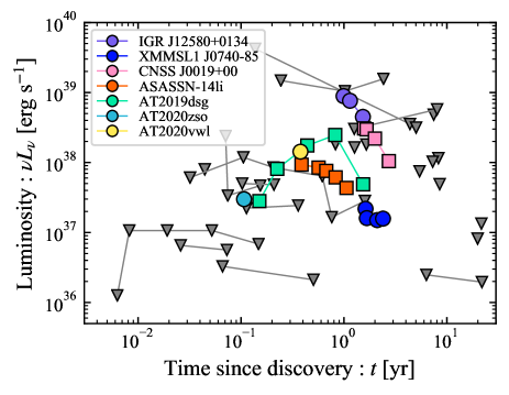
Figure 1: Radio light curves and upper limits of TDEs. The colored data points are detected events at frequency of $\nu\simeq 5\,\rm GHz$ and gray down triangles are upper limits. The squares (circles) mean the observations at which the spectral peak is (not) detected. On-axis jetted TDEs, Sw J1644+57, Sw J2058+05, and Sw J1112-82, whose radio luminosity is much larger $\sim 10^{40-42}\,\rm erg\,s^{-1}$, are not shown (see figure 1 in Alexander et al. 2020 for these events).

2 Method

2.1 Synchrotron emission

We describe the method to calculate the synchrotron flux based on Piran et al. (2013); Ricci et al. (2021). The CNM surrounding the BH in the TDEs is much denser than the interstellar medium around short gamma-ray bursts ($\lesssim 1\,\rm cm^{-3}$) and the synchrotron self-absorption (SSA) effect becomes important which shapes the observed spectrum. As most detected TDEs are at relatively small redshifts, we neglect the redshift effect in the following equations which can be easily restored. We consider an outflow traveling at a velocity $v$ in the CNM with the number density of $n$ at the shock front. The amplified magnetic field is given by an argument in which a fraction $\varepsilon_{\rm B}$ of the post-shock thermal energy is transferred to the magnetic field energy:

$$B =(8\pi\varepsilon_{\rm{B}}m_{\rm{p}}nv^{2})^{1/2}$$ (1)

$$\simeq 6.5\times 10^{-4}{\,\rm G\,}\varepsilon_{\rm B,-2}^{1/2}n_{0}^{1/2}v_{9},$$

where $m_{\rm{p}}$ is the proton mass. We use the notation $Q_{x}=Q/10^{x}$ in cgs units unless otherwise specified. A fraction $\varepsilon_{\rm e}$ of energy is also used to accelerate relativistic electrons in a power-law distribution. The minimum Lorentz factor of electrons and the corresponding synchrotron frequency are given by

$${\gamma}_{\rm{m}} ={\rm max}\biggl{[}2,\,\frac{m_{\rm{p}}}{4m_{\rm{e}}c^{2}}\bar{\varepsilon}_{\rm{e}}v^{2}\biggl{]}\simeq{\rm max}\big{[}2,\,0.051\,\bar{\varepsilon}_{\rm{e,-1}}v_{9}^{2}\big{]},$$ (2)

$${\nu}_{\rm{m}} ={\gamma}_{\rm{m}}^{2}\frac{eB}{2\pi m_{\rm{e}}c}$$ (3)

$$\simeq\begin{cases}7.2\times 10^{3}{\,\rm Hz\,}\,\varepsilon_{\rm B,-2}^{1/2}n_{0}^{1/2}v_{9}&:\,v<v_{\rm DN},\\ 4.7{\,\rm Hz\,}\,\bar{\varepsilon}_{\rm{e,-1}}^{2}\varepsilon_{\rm B,-2}^{1/2}n_{0}^{1/2}v_{9}^{5}&:\,v_{\rm DN}<v,\end{cases}$$

respectively, where $m_{\rm{e}}$ is the electron mass, $c$ is the speed of light, $e$ is the elementary charge, and we define $\bar{\varepsilon}_{\rm{e}}\equiv 4\varepsilon_{\rm{e}}(p-2)/(p-1)$ with the electron distribution’s power-law index $p$. When the outflow’s velocity is lower than the critical value

$$v<v_{\rm DN}=\biggl{(}\frac{8m_{\rm{e}}}{m_{\rm{p}}\bar{\varepsilon}_{\rm{e}}}\biggl{)}^{1/2}c\simeq 6.3\times 10^{4}{\,\rm km\,s^{-1}\,}\bar{\varepsilon}_{\rm{e,-1}}^{-1/2},$$ (4)

the Lorentz factor is fixed to ${\gamma}_{\rm{m}}=2$. We call this regime as the deep-Newtonian phase (Huang & Cheng, 2003; Sironi & Giannios, 2013). Hereafter we normalize the velocity by $10^{9}\,\rm cm\,s^{-1}$ regardless of each phase while an outflow with this velocity is in the deep-Newtonian phase.

The spectral power from an electron with the Lorentz factor ${\gamma}_{\rm{m}}$ is given by

$$P_{{\nu}_{\rm{m}}} \simeq\frac{\frac{4}{3}\sigma_{\rm{T}}c{\gamma}_{\rm{m}}^{2}\frac{B^{2}}{8\pi}}{{\nu}_{\rm{m}}}$$ (5)

$$\simeq 2.5\times 10^{-25}{\rm erg\,s^{-1}\,Hz^{-1}\,}\varepsilon_{\rm B,-2}^{1/2}n_{0}^{1/2}v_{9},$$

where $\sigma_{\rm T}$ is the Thomson cross section.

We estimate the number of electrons by

$$N_{\rm e}\simeq\Omega nR^{3},$$ (6)

where $\Omega$ is the solid angle subtended by the outflow. Examination of the Milky Way galactic center (Baganoff et al., 2003; Gillessen et al., 2019) as well as the analyses of radio TDEs (e.g. Alexander et al., 2016; Krolik et al., 2016) suggest that the CNM density in galactic nuclear regions has a power-law like profile, $n\propto R^{-k}$ ($k<3$), where $R$ is the distance from the BH. As we are not considering here the light curves but only the emission at some given moments of time we do not specify the density profile in this work but use instead only the density at the shock radius. As long as the density profile is shallow enough $k<3$, this estimate is accurate up to a numerical factor, $1/(3-k)$.

Noting that the number of radiating electrons is reduced by a factor of $(v/v_{\rm DN})^{2}$ in the deep-Newtonian phase, we calculate the flux density at ${\nu}_{\rm{m}}$

$$F_{{\nu}_{\rm{m}}} =\frac{N_{\rm e}\min\big{[}\big{(}\frac{v}{v_{\rm DN}}\big{)}^{2},\,1\big{]}P_{{\nu}_{\rm{m}}}}{4\pi d_{\rm L}^{2}}$$ (7)

$$\simeq\begin{cases}0.63{\,\rm\mu Jy\,}\bar{\varepsilon}_{\rm{e,-1}}\varepsilon_{\rm B,-2}^{1/2}n_{0}^{3/2}v_{9}^{3}R_{17}^{3}\big{(}\frac{\Omega}{4\pi}\big{)}d_{\rm L,27}^{-2}&:\,v<v_{\rm DN},\\ 25{\,\rm\mu Jy\,}\varepsilon_{\rm B,-2}^{1/2}n_{0}^{3/2}v_{9}R_{17}^{3}\big{(}\frac{\Omega}{4\pi}\big{)}d_{\rm L,27}^{-2}&:\,v_{\rm DN}<v,\end{cases}$$

where $N_{\rm e}$ and $d_{\rm L}$ are the total number of electrons and the luminosity distance, respectively.

The SSA frequency, which is typically larger than ${\nu}_{\rm{m}}$ for our parameters, is given by

$${\nu}_{\rm{a}} \simeq\biggl{(}\frac{(p-1)\pi^{\frac{3}{2}}3^{\frac{p+1}{2}}}{4}\frac{enR{\,\rm min}\big{[}\big{(}\frac{v}{v_{\rm DN}}\big{)}^{2},\,1\big{]}}{{\gamma}_{\rm{m}}^{5}B}\biggl{)}^{\frac{2}{p+4}}{\nu}_{\rm{m}}$$ (8)

$$\simeq\begin{cases}\big{(}4.0\times 10^{6}{\,\rm Hz}\big{)}_{p=2.5}\,\bar{\varepsilon}_{\rm{e,-1}}^{\frac{2}{p+4}}\\ \,\,\,\,\,\,\,\,\varepsilon_{\rm B,-2}^{\frac{p+2}{2(p+4)}}n_{0}^{\frac{p+6}{2(p+4)}}v_{9}^{\frac{p+6}{p+4}}R_{17}^{\frac{2}{p+4}}&:\,v<v_{\rm DN},\\ \big{(}2.3\times 10^{6}{\,\rm Hz}\big{)}_{p=2.5}\,\bar{\varepsilon}_{\rm{e,-1}}^{\frac{2(p-1)}{p+4}}\\ \,\,\,\,\,\,\,\,\varepsilon_{\rm B,-2}^{\frac{p+2}{2(p+4)}}n_{0}^{\frac{p+6}{2(p+4)}}v_{9}^{\frac{5p-2}{p+4}}R_{17}^{\frac{2}{p+4}}&:\,v_{\rm DN}<v.\end{cases}$$

Here in the second line we use $p=2.5$. We emphasize that hereafter when we estimate the numerical values we adopt $p=2.5$ and write the results with parentheses like $()_{p=2.5}$. Equations for general $p$ are given in Appendix A. For ${\nu}_{\rm{a}}>{\nu}_{\rm{m}}$, the synchrotron spectrum is given by

$$F_{\nu}=\begin{cases}F_{{\nu}_{\rm{m}}}({\nu}_{\rm{a}}/{\nu}_{\rm{m}})^{\frac{1-p}{2}}({\nu}_{\rm{m}}/{\nu}_{\rm{a}})^{5/2}(\nu/{\nu}_{\rm{m}})^{2}&:\nu<{\nu}_{\rm{m}},\\ F_{{\nu}_{\rm{m}}}({\nu}_{\rm{a}}/{\nu}_{\rm{m}})^{\frac{1-p}{2}}(\nu/{\nu}_{\rm{a}})^{5/2}&:{\nu}_{\rm{m}}<\nu<{\nu}_{\rm{a}},\\ F_{{\nu}_{\rm{m}}}(\nu/{\nu}_{\rm{m}})^{\frac{1-p}{2}}&:{\nu}_{\rm{a}}<\nu.\\ \end{cases}$$ (9)

In particular the spectral peak is given by at ${\nu}_{\rm{a}}$

$$F_{{\nu}_{\rm{a}}} =F_{{\nu}_{\rm{m}}}({\nu}_{\rm{a}}/{\nu}_{\rm{m}})^{\frac{1-p}{2}}$$ (10)

$$\simeq\begin{cases}\big{(}5.4\times 10^{-3}{\,\rm\mu Jy}\big{)}_{p=2.5}\,\bar{\varepsilon}_{\rm{e,-1}}^{\frac{5}{p+4}}\varepsilon_{\rm B,-2}^{\frac{2p+3}{2(p+4)}}\\ \,\,\,\,\,\,\,\,n_{0}^{\frac{2p+13}{2(p+4)}}v_{9}^{\frac{2p+13}{p+4}}R_{17}^{\frac{2p+13}{p+4}}\big{(}\frac{\Omega}{4\pi}\big{)}d_{\rm L,27}^{-2}&:\,v<v_{\rm DN},\\ \big{(}1.3\times 10^{-3}{\,\rm\mu Jy}\big{)}_{p=2.5}\,\bar{\varepsilon}_{\rm{e,-1}}^{\frac{5(p-1)}{p+4}}\varepsilon_{\rm B,-2}^{\frac{2p+3}{2(p+4)}}\\ \,\,\,\,\,\,\,\,n_{0}^{\frac{2p+13}{2(p+4)}}v_{9}^{\frac{12p-7}{p+4}}R_{17}^{\frac{2p+13}{p+4}}\big{(}\frac{\Omega}{4\pi}\big{)}d_{\rm L,27}^{-2}&:\,v_{\rm DN}<v,\end{cases}$$

and the flux density in ${\nu}_{\rm{a}}<\nu$ and ${\nu}_{\rm{m}}<\nu<{\nu}_{\rm{a}}$, which are the relevant regimes in our study, are given by

$$F_{\nu>{\nu}_{\rm{a}}} =F_{{\nu}_{\rm{a}}}(\nu/{\nu}_{\rm{a}})^{\frac{1-p}{2}}$$ (11)

$$\simeq\begin{cases}\big{(}3.8\times 10^{-5}{\,\rm\mu Jy}\big{)}_{p=2.5}\,\bar{\varepsilon}_{\rm{e,-1}}\varepsilon_{\rm B,-2}^{\frac{p+1}{4}}\\ \,\,\,\,\,\,\,\,n_{0}^{\frac{p+5}{4}}v_{9}^{\frac{p+5}{2}}R_{17}^{3}\big{(}\frac{\Omega}{4\pi}\big{)}\nu_{\rm 3GHz}^{\frac{1-p}{2}}d_{\rm L,27}^{-2}&:\,v<v_{\rm DN},\\ \big{(}6.1\times 10^{-6}{\,\rm\mu Jy}\big{)}_{p=2.5}\,\bar{\varepsilon}_{\rm{e,-1}}^{p-1}\varepsilon_{\rm B,-2}^{\frac{p+1}{4}}\\ \,\,\,\,\,\,\,\,n_{0}^{\frac{p+5}{4}}v_{9}^{\frac{5p-3}{2}}R_{17}^{3}\big{(}\frac{\Omega}{4\pi}\big{)}\nu_{\rm 3GHz}^{\frac{1-p}{2}}d_{\rm L,27}^{-2}&:\,v_{\rm DN}<v,\end{cases}$$

$$F_{\nu<{\nu}_{\rm{a}}} =F_{{\nu}_{\rm{a}}}(\nu/{\nu}_{\rm{a}})^{\frac{5}{2}}$$ (12)

$$\simeq 8.2\times 10^{4}{\,\rm\mu Jy\,}\varepsilon_{\rm B,-2}^{-1/4}n_{0}^{-1/4}v_{9}^{-1/2}R_{17}^{2}\biggl{(}\frac{\Omega}{4\pi}\biggl{)}\nu_{\rm 3GHz}^{5/2}d_{\rm L,27}^{-2},$$

respectively, where $\nu_{\rm 3GHz}=\nu/3\,\rm{GHz}$. Note that the flux density for ${\nu}_{\rm{m}}<\nu<{\nu}_{\rm{a}}$ (Eq. 12) has a common dependence on the parameters for the both regimes.

2.2 Radio constraints

We constrain the outflow’s properties such as velocity $v$ and solid angle $\Omega$ and the CNM density $n$ by using the radio observations. The radius of the outflow is approximately estimated by $R\simeq vt$. Strictly speaking, the radius is given not by the outflow velocity $v$ but by the shock velocity, which is slightly larger than $v$. This approximation holds even after the outflow starts to decelerate. For instance, with a density profile of $n\propto R^{-k}$ ($k<3$), the radius and velocity evolve as $R\propto t^{2/(5-k)}$ and $v\simeq dR/dt$, respectively, which gives $R\simeq[(5-k)/2]vt$. These numerical factors do not change our results significantly as long as we take $v$ as a fundamental quantity (instead of $R$). Here $t$ is the time measured since the outflow launch. Therefore, the synchrotron flux is determined by three key parameters of $v$, $\Omega$, and $n$. By substituting $R=vt$ to Eqs. (11) and (12) and setting the flux smaller than the upper limit $F_{\nu}$ at frequency $\nu$, we constrain the combinations of the parameters for optically thin and the deep-Newtonian phase ($v<v_{\rm DN}$),

$$n_{0}^{\frac{p+5}{4}}v_{9}^{\frac{p+11}{2}}\Omega\lesssim\big{(}3.2\times 10^{8}\big{)}_{p=2.5}\,\bar{\varepsilon}_{\rm{e,-1}}^{-1}\varepsilon_{\rm B,-2}^{-\frac{p+1}{4}}t_{\rm yr}^{-3}\nu_{\rm 3GHz}^{\frac{p-1}{2}}d_{\rm L,27}^{2}F_{\rm 30\mu Jy},$$ (13)

for optically thin and $v>v_{\rm DN}$ case,

$$n_{0}^{\frac{p+5}{4}}v_{9}^{\frac{5p+3}{2}}\Omega\lesssim\big{(}2.0\times 10^{9}\big{)}_{p=2.5}\,\bar{\varepsilon}_{\rm{e,-1}}^{1-p}\varepsilon_{\rm B,-2}^{-\frac{p+1}{4}}t_{\rm yr}^{-3}\nu_{\rm 3GHz}^{\frac{p-1}{2}}d_{\rm L,27}^{2}F_{\rm 30\mu Jy},$$ (14)

and for the optically thick case,

$$n_{0}^{-1/4}v_{9}^{3/2}\Omega\lesssim 4.6\times 10^{-3}\,\varepsilon_{\rm B,-2}^{1/4}t_{\rm yr}^{-2}\nu_{\rm 3GHz}^{-5/2}d_{\rm L,27}^{2}F_{\rm 30\mu Jy},$$ (15)

where $t_{\rm yr}=t/\rm yr$ and $F_{30\mu\rm Jy}=F_{\nu}/\rm 30\,\mu Jy$. In particular, the velocity is constrained by

$$v\lesssim\begin{cases}\big{(}1.8\times 10^{5}{\,\rm km\,s^{-1}\,}\big{)}_{p=2.5}\,\Big{[}\bar{\varepsilon}_{\rm{e,-1}}^{-1}\varepsilon_{\rm B,-1}^{-\frac{p+1}{4}}\\ \,\,\,t_{\rm yr}^{-3}\nu_{\rm 3GHz}^{\frac{p-1}{2}}d_{\rm L,27}^{2}F_{\rm 30\mu Jy}n_{0}^{-\frac{p+5}{4}}\Omega^{-1}\Big{]}^{\frac{2}{p+11}}&:{\rm thin\,}(v<v_{\rm DN}),\\ \big{(}1.6\times 10^{5}{\,\rm km\,s^{-1}\,}\big{)}_{p=2.5}\,\Big{[}\bar{\varepsilon}_{\rm{e,-1}}^{1-p}\varepsilon_{\rm B,-2}^{-\frac{p+1}{4}}\\ \,\,\,t_{\rm yr}^{-3}\nu_{\rm 3GHz}^{\frac{p-1}{2}}d_{\rm L,27}^{2}F_{\rm 30\mu Jy}n_{0}^{-\frac{p+5}{4}}\Omega^{-1}\Big{]}^{\frac{2}{5p+3}}&:{\rm thin\,}(v>v_{\rm DN}),\\ 1.3\times 10^{3}{\,\rm km\,s^{-1}\,}\,\varepsilon_{\rm B,-2}^{1/6}t_{\rm yr}^{-4/3}\nu_{\rm 3GHz}^{-5/3}\\ \,\,\,d_{\rm L,27}^{4/3}F_{\rm 30\mu Jy}^{2/3}n_{0}^{1/6}\Omega^{2/3}&:{\rm thick},\end{cases}$$ (16)

corresponding to Eqs. (13), (14), and (15), respectively. Fig. 2 depicts an example demonstrating how a radio upper-limit constrains the density and velocity space for a given $\Omega$.

The spectrum peaks at ${\nu}_{\rm{a}}$ and this implies that regardless of the external density, a minimal velocity is required to realize a given flux for a given $\Omega$. The minimal velocity is obtained by equating the observed flux (upper limit) and frequency with $F_{{\nu}_{\rm{a}}}$ and ${\nu}_{\rm{a}}$ (Eqs. 8 and 10), or equivalently given by the intersection of the velocity limits at the optically thin and thick regimes (Eqs. 16). The minimal velocity and the corresponding density are given by

$$v_{\rm eq} \simeq\begin{cases}\big{(}8.3\times 10^{3}{\,\rm km\,s^{-1}\,}\big{)}_{p=2.5}\,\,\bar{\varepsilon}_{\rm{e,-1}}^{-\frac{1}{2p+13}}\varepsilon_{\rm B,-2}^{\frac{1}{2p+13}}\\ \,\,\,\,\,\,t_{\rm yr}^{-1}\nu_{\rm 3GHz}^{-1}d_{\rm L,27}^{\frac{2(p+6)}{2p+13}}F_{\rm 30\mu Jy}^{\frac{p+6}{2p+13}}\Omega^{-\frac{p+6}{2p+13}}&:v<v_{\rm DN},\\ \big{(}9.2\times 10^{3}{\,\rm km\,s^{-1}\,}\big{)}_{p=2.5}\,\bar{\varepsilon}_{\rm{e,-1}}^{\frac{1-p}{4p+9}}\varepsilon_{\rm B,-2}^{\frac{1}{4p+9}}\\ \,\,\,\,\,\,t_{\rm yr}^{-\frac{2p+13}{4p+9}}\nu_{\rm 3GHz}^{-\frac{2p+13}{4p+9}}d_{\rm L,27}^{\frac{2(p+6)}{4p+9}}F_{\rm 30\mu Jy}^{\frac{p+6}{4p+9}}\Omega^{-\frac{p+6}{4p+9}}&:v>v_{\rm DN}.\end{cases}$$ (17)

$$n_{\rm eq} \simeq\begin{cases}\big{(}6.8\times 10^{4}{\,\rm cm^{-3}}\big{)}_{p=2.5}\bar{\varepsilon}_{\rm{e,-1}}^{-\frac{6}{2p+13}}\varepsilon_{\rm B,-2}^{-\frac{2p+7}{2p+13}}\\ \,\,\,\,\,\,t_{\rm yr}^{2}\nu_{\rm 3GHz}^{4}d_{\rm L,27}^{-\frac{4(p+8)}{2p+13}}F_{\rm 30\mu Jy}^{-\frac{2(p+8)}{2p+13}}\Omega^{\frac{2(p+8)}{2p+13}}&:v<v_{\rm DN},\\ \big{(}1.3\times 10^{5}{\,\rm cm^{-3}\,}\big{)}_{p=2.5}\bar{\varepsilon}_{\rm{e,-1}}^{\frac{6(1-p)}{4p+9}}\varepsilon_{\rm B,-2}^{-\frac{4p+3}{4p+9}}\\ \,\,\,\,\,\,t_{\rm yr}^{\frac{2(10p-3)}{4p+9}}\nu_{\rm 3GHz}^{\frac{4(7p+3)}{4p+9}}d_{\rm L,27}^{-\frac{20p}{4p+9}}F_{\rm 30\mu Jy}^{-\frac{10p}{4p+9}}\Omega^{\frac{10p}{4p+9}}&:v>v_{\rm DN},\end{cases}$$ (18)

respectively. At $R_{\rm eq}\equiv v_{\rm eq}t$ and $n_{\rm eq}$ the upper limit corresponds to the spectral peak at $\nu_{\rm a}$. Hence in particular for the case of $v_{\rm eq}<v_{\rm DN}$ the radius $R_{\rm eq}$ is comparable to the equipartition radius (e.g. Chevalier, 1998; Barniol Duran et al., 2013). Strictly speaking, our “equipartition” radius minimizes the total energy in the emitting site (including all electrons’ energy). Note we allow for a general relations $\varepsilon_{\rm B}\ll\varepsilon_{\rm e}$ (see also Chevalier, 1998) while the literal equipartition is realized with $\varepsilon_{\rm B}=(6/11)\varepsilon_{\rm e}$ at the equiaprtition radius of Barniol Duran et al. (2013). This of course results in that our total energy is slightly larger, but the radius remains practically unchanged.

There is more important difference between our method and the usual application of the equipartition method (Chevalier, 1998; Barniol Duran et al., 2013). The equipartition method is applicable only when the spectral peak is observed. On the other hand, our formulation can be applied to any observations.

Additionally the density $n_{\rm eq}$ that we find is typically 30-100 times larger than the one obtained by the equipartition method. This is because we take into account the fact that only a fraction $(v/v_{\rm DN})^{2}\simeq 1-3\,\%$ of the electrons participates in the power-law distribution in the deep-Newtonian phase, that is usually not considered in the simple version of the equipartition calculations.

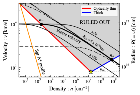
Figure 2: Example of the constraint on the density and velocity space by a typical radio upper-limit of $F_{\nu}=30\,\rm\mu Jy$ at $\nu=3\,\rm GHz$ for $z=0.072$ ($d_{\rm L}=10^{27}\,\rm cm$) and $t=3\,\rm yr$. Red and blue lines represent the boundaries of the excluded (gray) region imposed by the optically thin ($\nu>{\nu}_{\rm{a}}$) and thick ($\nu<{\nu}_{\rm{a}}$) regimes, respectively. The adopted parameters are $\bar{\varepsilon}_{\rm{e}}=0.1$, $\varepsilon_{\rm{B}}=0.01$, $p=2.5$, and $\Omega=4\pi$. The intersection of two lines (star) gives the minimal velocity $v_{\rm eq}$ corresponding to the equipartition radius $R_{\rm eq}(=v_{\rm eq}t)$. The thick-black-solid curve denotes the trajectory of shock velocity given by solving Eq. (19) for $M_{\rm ej}=0.5\,\mathrm{M}_{\odot}$ and $v_{\rm in}=10^{4}\,\rm km\,s^{-1}$. The thin-black-solid curves show trajectories with the same $v_{\rm in}$ but 30 times larger and smaller $E_{\rm kin}$ (or equivalently $M_{\rm ej}$). The black dash-dotted curves represent trajectories with the same $E_{\rm kin}$ but 3 times higher and lower $v_{\rm in}$. For large density, these curves with the same $E_{\rm kin}$ approach to the black-dotted line $v\propto n^{-1/5}$, which corresponds to decelerating jets. Within the outflow model, any density profile intersecting the trajectory within the ruled-out region for $n_{-}\leq n\leq n_{+}$ is excluded. The density profile of Sgr A* (orange line, $n\simeq 10\,{\rm cm^{-3}}(R/10^{18}\,\rm cm)^{-1}$, Baganoff et al. 2003; Gillessen et al. 2019) is allowed by the model.

2.3 Outflow model

Consider an outflow launched into a solid angle $\Omega$. Generally, the outflow is ejected with a range of velocities and we denote the mass moving at larger velocity than $v$ as $M_{\rm ej}(>v)$ and its corresponding kinetic energy as $E_{\rm kin}(>v)$. At a given moment, the shock velocity of the outflow $v$ is determined by the energy conservation (Piran et al., 2013):

$${E}_{\rm{kin}}(>v) =\big{[}{M}_{\rm{ej}}(>v)+M(R)\big{]}v^{2}/2,$$ (19)

where the swept-up CNM mass is approximated as in Eq. (6):

$$M(R)\simeq\Omega m_{\rm{p}}nR^{3}.$$ (20)

The shock radius is reasonably given by $R\simeq vt$.

As a simple example, we consider an outflow characterized by a single initial velocity $v_{\rm in}$ with mass $M_{\rm ej}$, kinetic energy $E_{\rm kin}=M_{\rm ej}v_{\rm in}^{2}/2$, and angle $\Omega=4\pi$. Fig. 2 depicts trajectories of velocity obtained by solving Eq. (19) for different densities at the shock front. For small CNM density, the outflow is still traveling with its initial velocity (free expansion). When the swept-up CNM mass is larger than the outflow’s mass, its velocity decreases. The trajectory asymptotes to a line, $v\propto n^{-1/5}$ which is obtained by neglecting the outflow mass (${M}_{\rm{ej}}\to 0$). As we will see in §4, this line represents the trajectory of decelerating jets and its normalization is determined only by the outflow’s kinetic energy.

When the outflow velocity is larger than the minimal velocity $v_{\rm eq}$ corresponding to a given upper limit on $F_{\nu}$, the trajectory intersects the excluded region for $n_{-}<n<n_{+}$. Here we define $n_{+}$ and $n_{-}$ as the densities at the intersections with the optically thick and thin boundaries, respectively (see Fig. 2). We find that for most cases, the density $n_{+}$ is much larger than the relevant CNM-density range. Hence we only consider the branch of $n<n_{-}$, where $n_{-}$ gives an upper limit on the density. As long as we consider the density limit in the optically thin regime $n_{-}$, the outflow velocity does not change significantly from the initial value $v_{\rm in}$. Therefore the limiting density depends on $\varepsilon_{\rm B}$, $v_{\rm in}$ and $\Omega$ as

$$n_{-}\propto\varepsilon_{\rm B}^{-\frac{p+1}{p+5}}v_{\rm in}^{-\frac{2(p+11)}{p+5}}\Omega^{-\frac{4}{p+5}}\simeq\varepsilon_{\rm B}^{-0.47}v_{\rm in}^{-3.6}\Omega^{-0.53},$$ (21)

where the last equality holds for $p=2.5$.

In the following calculations we adopt $\bar{\varepsilon}_{\rm e}=0.1$, $\varepsilon_{\rm B}=0.01$, $p=2.5$ as the fiducial values (several radio detected events have different $p$, see Table 2). The value of $\varepsilon_{\rm B}$ is not well constrained by the observations and can vary for different events shifting the boundary of the ruled-out region in Fig. 2.

To summarize this section we note that when a radio signal is detected this immediately gives a lower limit on the velocity $v_{\rm eq}$ or equivalently the combination of $v\Omega^{a}$ where $a=(p+6)/(2p+13)\simeq 0.47$ for $p=2.5$ ($v<v_{\rm DN}$) or $a=(p+6)/(4p+9)\simeq 0.45$ for $p=2.5$ ($v>v_{\rm DN}$). This limit is independent of the density. For an upper limit on the radio flux, we obtain a forbidden region in $n$ and $v$ space as a function of $\Omega$. Given an outflow model, we can constrain the density. Alternatively, once a density profile is specified, we can constrain the outflow’s properties such as $v$ and $\Omega$.

A give outflow is characterized by its geometry, mass, and velocity (actually by $M_{\rm ej}(>v)$). Among these three parameters, with a detection we have a direct bound on the product of two $v\Omega^{a}$ (as described above). The total mass is less important as typically only a small fraction of it is sufficient to power the observed signal. However, as we show later its velocity distribution might be critical.

Going back to Fig. 2, we note that the density and velocity in the shaded region are ruled out for an upper limit. For a detection without an SSA spectral peak, its parameters should be on the boundary of the ruled-out region. Only when the spectral peak is detected the parameters are determined on the bottom of the boundary (a star), which is the usual equipartition method.

3 Application to Astrophysical Models

We turn now to apply the method developed in §2 to four different possible sources of the flare. These are distinguished by their geometry, typical masses, and expected velocities.

Disk winds, that arise if circularization takes place rapidly and a super-Eddington emitting disk forms, have a quasi spherical geometry. The unbound disrupted stellar mass has a wedge-like geometry while a possible Newtonian jet will have a conical shape. Among the three only for the disrupted stellar mass we have estimates of the mass-velocity distribution, $M_{\rm ej}(>v)$. For the disk wind we can expect the velocity to be of order of (or larger than) the escape velocity from the photosphere of several thousand $\rm km\,s^{-1}$ (e.g. Matsumoto & Piran, 2021). For Newtonian jets considered within this context of TDE radio emission (see e.g. Alexander et al., 2016), its mass, velocity, and even the opening angle are typically not constrained by other considerations.

3.1 Spherical outflow - Disk Wind

First we consider a spherical outflow. Such an outflow can arise from a disk wind. If circularization is efficient, a compact accretion disk forms rapidly after the bound debris returns to the pericenter. Since the mass fallback rate is well above the Eddington rate, a strong disk wind could emerge and carry out a significant mass (Blandford & Begelman, 1999). The wind plays a role of an envelope surrounding the disk and absorbing the disk’s X-rays to reprocess to optical light (Loeb & Ulmer, 1997; Metzger & Stone, 2016; Roth et al., 2016). Recently we have shown that the observations imply that such winds are too massive and would carry out more than the available mass (Matsumoto & Piran 2021, see also Uno & Maeda 2020). Naturally a radio signal is expected from the interaction of such a wind with the CNM and null detection of radio emission from TDEs provides an independent constrain on this scenario.

Consider an isotropic ($\Omega=4\pi$) outflow characterized by a single (initial) velocity $v_{\rm in}=10^{4}\,\rm km\,s^{-1}$ and mass ${M}_{\rm{ej}}=0.5\,\mathrm{M}_{\odot}$ (as we discuss later as the energy emitted by the shock is very small, the outcome does not depend on the total mass as long as it is sufficiently larger than the swept-up mass, $M_{\rm ej}>M(R)$). These values follow from the reprocessed model (e.g. Metzger & Stone, 2016) and considered in §2.3 as an example. The shock radius is approximately given by $R\simeq vt$, and the time is measured since the wind launch. For $t$, we use, here and in the rest of the paper, the time measured since the discovery of TDEs, which is a reasonable approximation because the radio observation times are typically late. For a given time and CNM density at the shock front, the shock velocity is given by Eq. (19). Fig. 2 depicts trajectories of the outflow velocity with the corresponding excluded parameter space obtained by a typical radio upper-limit of $F_{\nu}=30\,\mu\rm Jy$ at $\nu=3\,\rm GHz$ for $z=0.072$ ($d_{\rm L}=10^{27}\,\rm cm$) and $t=3\,\rm yr$.

For each radio upper-limit in Fig. 1, we calculate the quantities $v_{\rm eq}$, $n_{\rm eq}$, $v_{-}$, and $n_{-}$ (corresponding to the optically thin regime) assuming $p=2.5$ and tabulate them in Table 1. Fig. 3 depicts the upper limits on the density $n_{-}$ at the distance $R=v_{-}t$ when the limiting velocity is larger than the critical velocity $v_{-}>v_{\rm eq}$. Due to the large solid angle, which minimizes the minimal-required velocity $v_{\rm eq}$, we obtain meaningful and strongest constraints (see below for the cases of $\Omega<4\pi$). It is the late upper-limits ($>10\,\rm yr$) that give the strongest limits (furthest away from the BH and hence the expected density is lowest). As seen in Eq. (21), increasing the velocity by a factor of 2, which is the case of the high tail of the velocity distribution, will decrease the density limit about ten times. Limits are meaningful compared to the density profile seen in the radio-detected TDEs. These results do not rule out the strong disk wind scenario such as the reprocessed optical-emission model.

For radio-detected TDEs, the wind interaction with the CNM can be an efficient radio source provided that its velocity is not too small ($v_{\rm in}\gtrsim 10^{4}\,\rm km\,s^{-1}$). For three radio TDEs with a spectral peak (CNSS J0019+00, ASASSN-14li, and AT2019dsg), we estimate the densities $n_{\rm eq}$ corresponding to the minimal velocities $v_{\rm eq}$. For these events, observations at different times show that the outflow does not decelerate (see Table 2). This, in turn, suggests the outflow mass is larger than the swept-up CNM mass: $M_{\rm ej}\gtrsim M(R)\simeq 0.01-0.1\,\mathrm{M}_{\odot}$ (as shown in Fig. 3). Hence the outflow’s kinetic energy should be larger than $E_{\rm kin}\gtrsim v_{\rm eq}^{2}M(R)/2\simeq 10^{49-50}\,\rm erg$.

The densities that we find here are 30-100 times larger than those obtained by previous works based on the equipartition method (Alexander et al., 2016; Krolik et al., 2016; Anderson et al., 2020; Stein et al., 2021; Cendes et al., 2021a), because these works considered only the number of relativistic electrons, which is typically smaller by a factor of $(v/v_{\rm DN})^{2}$ than the total electron density in the deep-Newtonian phase. Accordingly their estimates of outflow’s mass and kinetic energy are smaller than ours by the similar factor. The number density obtained by Yalinewich et al. (2019) for ASASSN-14li (after correcting the difference of solid angle) is also slightly ($\sim 3$ times) smaller than ours because they assumed the fraction of accelerated electrons $10\,\%$.

We carry out similar calculations for radio-detected TDEs without a spectral peak. Assuming an initial velocity $v_{\rm in}=10^{4}\,\rm km\,s^{-1}$ we find that the wind velocity does not vary during the observations. The outflow mass is hence bounded by the swept-up mass and can be small such as $M_{\rm ej}\gtrsim M(R)\simeq 0.03\,\mathrm{M}_{\odot}$ and the minimal energy becomes $E_{\rm kin}\gtrsim 3\times 10^{49}{\,\rm erg\,}M_{\rm ej,-1.5}v_{\rm in,9}^{2}$. Some of the radio-detected TDEs require densities larger than those of radio upper-limits TDEs. This suggests that either not every TDE is accompanied by a disk wind or the CNM profiles vary significantly among galaxies.

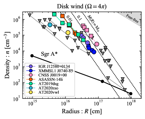
Figure 3: Limits or required CNM density by the radio observations for the case of a spherical outflow ($\Omega=4\pi$, $M_{\rm ej}=0.5\,\mathrm{M}_{\odot}$, and $v_{\rm in}=10^{4}\,\rm km\,s^{-1}$). Down-triangles, circles, and squares represent the upper limits on the density by radio limits, required density by radio TDEs without spectral peak, and density obtained by the equipartition method, respectively. Upper limits at large radius correspond to the radio limits at late time. The dashed lines show the locations where the enclosed masses are $M(R)=10^{-3}-10^{-1}\,\mathrm{M}_{\odot}$. If the outflow mass is larger than $M(R)$, it does not decelerate significantly. The black line represents the density profile of Sgr A* (Baganoff et al. 2003; Gillessen et al. 2019). In the upper right shaded region, the free-free absorption reduces the observed flux (assumed the virial temperature for $M_{\rm BH}=10^{6.5}\,\mathrm{M}_{\odot}$) at $\nu=1\,\rm GHz$.

3.2 Wedge geometry - Unbound debris

3.2.1 Dynamics of unbound debris

About half of the stellar mass torn apart in a TDE is ejected as unbound debris. The interaction of the debris with the CNM should produce radio emission. We turn, now, to constrain the debris properties and the CNM density using the radio observations.

We consider a disruption event of a star with mass $M_{*}$ and radius $R_{*}$ by a BH with mass $M_{\rm BH}$. After the disruption, the stellar debris has a flat distribution over specific energy within a characteristic energy of $\Delta\epsilon\equiv(GM_{\rm BH}R_{*}/R_{\rm T}^{2})\Xi$, where $G$ is the gravitational constant and $R_{\rm T}\equiv R_{*}(M_{\rm BH}/M_{*})^{1/3}$ is the tidal radius. $\Xi$ is a numerical factor derived by Ryu et al. (2020) in order to include corrections arising due to the internal stellar structure and relativistic effects. This correction is less than a factor of $2$ for typical values and it becomes $\Xi\simeq 1.3$ for a star with $M_{\odot}$ and BH with $M_{\rm BH}=10^{6.5}\,\mathrm{M}_{\odot}$. The corresponding typical velocity is

$${\cal V}=\sqrt{2\Delta\varepsilon}\simeq 8600{\,\rm km\,s^{-1}\,}R_{*,0}^{-1/2}M_{*,0}^{1/3}M_{\rm BH,6.5}^{1/6}(\Xi/1.3)^{1/2}\ ,$$ (22)

where we normalize the radius and mass by solar values. As a zeroth order approximation we could consider outflow with mass $M_{\rm ej}\simeq 0.5\,\mathrm{M}_{\odot}$ and an opening angle of $\Omega\sim 0.1$ (as discussed later) with this velocity. However, Ryu et al. (2020) also found the detailed specific-energy distribution. This distribution has a tail beyond $\Delta\epsilon$ whose shape can be approximated by an exponential. Since the small fraction of fast unbound debris can contribute to or even dominate a radio flare (Krolik et al., 2016; Yalinewich et al., 2019), we take this structure into account and adopt the following distribution

$$\frac{dM}{d\epsilon} =\frac{\alpha M_{*}}{2(\alpha+1)\Delta\epsilon}\begin{cases}1&:\epsilon<\Delta\epsilon\ ,\\ \exp\Big{[}-\alpha\Big{(}\frac{\epsilon-\Delta\epsilon}{\Delta\epsilon}\Big{)}\Big{]}&:\epsilon>\Delta\epsilon\ ,\\ \end{cases}$$ (23)

where the slope of the exponential tail $\alpha\gtrsim 3$ depends on the type of the disrupted star (Ryu et al., 2020) and we use $\alpha=3$ as a fiducial value. The normalization is determined so that the total unbound mass for $\epsilon>0$ becomes $M_{*}/2$. With a relation $\epsilon=v^{2}/2$, the debris mass and kinetic energy distributions over velocity are given by $d{M}_{\rm{ej}}/dv=v(dM/d\epsilon)$ and $d{E}_{\rm{kin}}/dv=(v^{2}/2)(d{M}_{\rm{ej}}/dv)$, respectively. Fig. 4 depicts the cumulative mass and kinetic energy profiles of the debris, $M_{\rm ej}(>v)$ and $E_{\rm kin}(>v)$. The total kinetic energy is given by ${E}_{\rm{kin}}\simeq 2.6\times 10^{50}{\,\rm erg\,}R_{*,0}M_{*,0}^{5/3}M_{\rm BH,6.5}^{1/3}$ for $\alpha=3$. Only a small fraction of debris has a larger velocity $v\gtrsim 10^{4}\,\rm km\,s^{-1}$.

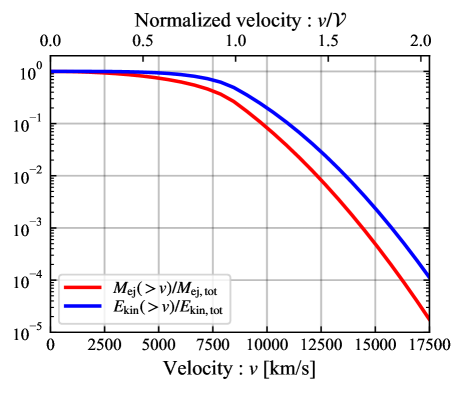
Figure 4: Cumulative mass and kinetic energy of unbound debris (reconstructed from the specific energy distribution, Eq. 23) for parameters of $M_{\rm*}=\mathrm{M}_{\odot}$ ($R_{*}=R_{\odot}$), $M_{\rm BH}=10^{6.5}\,\mathrm{M}_{\odot}$, and $\alpha=3$. The velocity normalization $\cal V$ is given by Eq. (22).

The dynamics of the unbound debris is determined by using Eq. (19) and the mass and energy distributions. The debris expands in a wedge geometry like a fan (constant ratio of the width to radius $H/R$, Strubbe & Quataert, 2009; Yalinewich et al., 2019) producing a bow shock with a typical solid angle of $\Omega\sim 0.1$ (Yalinewich et al., 2019). At first, the faster and less massive debris travels ahead of the whole debris and its bow shock dominates the radio emission. As it decelerates, more massive debris dominates. At a given moment, the emission mainly comes from the bow shock formed by the debris which just begins to decelerate. The shock velocity is comparable to the debris velocity.

Fig. 5 depicts the debris velocity as a function of the density at the shock front. The energy and mass profiles are calculated by the distribution given by Eq. (23) (see also Fig. 4). We approximate the radius $R\simeq vt$. As the debris sweeps up CNM and decelerates, it expands sideways and increases the solid angle of the bow shock $\Omega$. The expanding part sweeps up more CNM and decelerates faster. We do not include this sideways expansion in our estimate and we assume the constant angle because the rapidly decelerating part does not contribute to the emission significantly (note that in the optically thin regime the flux sensitively depends on the velocity, Eq. 11 and see an argument in Margalit & Piran 2015).

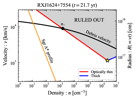
Figure 5: The same as Fig. 2 but for the radio upper-limit of RXJ1624+7554 at $t=21.6\,\rm yr$ in the case of unbound debris with a solid angle $\Omega=0.1$. The black curve denotes the velocities of the unbound debris and its bow shock as a function of the density given by Eq. (19) with the profile of Eq. (23), for given debris mass $M_{\rm ej}=0.5\,\mathrm{M}_{\odot}$, kinetic energy $E_{\rm kin}\simeq 3\times 10^{50}\,\rm erg$, and BH mass $M_{\rm BH}=10^{6.5}\,\mathrm{M}_{\odot}$.

3.2.2 Observational constraints

We derive the constraint in the context of unbound debris. Fig. 5 shows the ruled-out parameter space for the null detection in RXJ1624+7554 at $t=21.6\,\rm yr$ (shown in the first line of Table 1). In this example, any velocity below $v_{\rm eq}\simeq 10^{3}\,\rm km\,s^{-1}$ is allowed (for this assumed $\Omega$). The velocity trajectory overlaps the ruled-out region and the flux upper-limit requires the density smaller than $n<n_{-}\simeq 10^{3}\,\rm cm^{-3}$.

Fig. 6 depicts the resulting upper limits on the density $n_{-}$. In order to calculate the debris velocity, we adopt the same parameters of $M_{*}=\mathrm{M}_{\odot}$, $R_{*}=R_{\odot}$, and $M_{\rm BH}=10^{6.5}\,\mathrm{M}_{\odot}$. Using the same BH mass for all events is reasonably justified because the characteristic velocity weakly depends on this parameter (see Eq. 22). With this fiducial debris model, only half of the TDEs with upper limits gives meaningful constraints on the density. These density limits are all larger than the CNM density in Sgr A*. The other half does not produce a radio flare as bright as the upper limit because its velocity is smaller than the minimal one $v_{\rm eq}$.

For TDEs with a spectral peak (CNSS J0019+00, ASASSN-14li and AT2019dsg), if the peak is caused by SSA, the velocity and density should be equal to $v_{\rm eq}$ and $n_{\rm eq}$ as obtained by the equipartition method. However, with the solid angle of $\Omega=0.1$, the minimal velocities are typically larger than that of the unbound debris $v_{\rm eq}\gtrsim 10^{4}\,\rm km\,s^{-1}$. With these parameters of our fiducial debris model the unbound debris cannot be the radio source in these events. Similarly, for radio TDEs without a spectral peak only XMMSL J0740-85 can be powered by unbound debris in our model (see Fig. 6). These limits are slightly relaxed if we take into account that the shock velocity is larger than the fluid velocity. But this is not sufficient to fully resolve the discrepancy.

Generally speaking, the radio emission from unbound debris is much dimmer than the other outflow components because of its small solid angle, $\Omega\sim 0.1$. The angle can be ten times larger than the fiducial value, $\Omega\sim 1$ for TDEs in which the stellar pericenter is smaller than the tidal radius as studied by Yalinewich et al. (2019) for modeling of ASASSN-14li. In such TDEs, the luminosity becomes $\sim 10$ times larger and the equipartition velocity is also reduced by a factor three, $v_{\rm eq}\propto\Omega^{-\frac{p+6}{2p+13}}\simeq\Omega^{-0.47}$ for $p=2.5$, which results in more events give meaningful constraints on the density. With this scaling, we find that debris should have a distribution in which at least $\sim 10^{-2}\,\mathrm{M}_{\odot}$ of mass moves at $\gtrsim 2\times 10^{4}\,\rm km\,s^{-1}$.

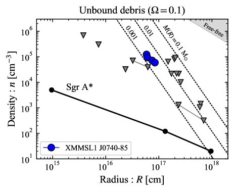
Figure 6: The same as Fig. 3 but for the case of unbound debris ($\Omega=0.1$, $M_{*}=\mathrm{M}_{\odot}$, and $M_{\rm BH}=10^{6.5}\,\mathrm{M}_{\odot}$). The dashed lines show the locations where the enclosed masses are $M(R)=10^{-3}-10^{-1}\,\mathrm{M}_{\odot}$ (see Eq. 20).

3.3 Conical outflow - a Newtonian Jet

We turn now to conical outflows that are launched with sub-relativistic velocities (e.g. Alexander et al., 2016). Such a jet-like structure can arise, for example, from a disk wind that has a strong angular structure. Lacking a specific model for generation of such a jet, here, unlike the previous two cases we do not have specific model parameters to compare with and all that can be done is to infer jet parameters that fit the data. Naturally, this is almost always possible. Relativistic jets behave differently and we consider those in the next section.

As the jet propagates in the surrounding CNM its energy is dissipated at the head and a hot cocoon forms (see e.g. Begelman & Cioffi, 1989; Bromberg et al., 2012). The effective width of the emitting region of the jet is therefore larger, but comparable, to its original width. Namely, $\Omega\gtrsim 2\pi\theta^{2}$, where $\theta$ is the original jet half-opening angle.

As long as jet’s mass is larger than the swept-up CNM mass, it does not decelerate. In this case we can simply follow the analysis in §3.1 using the assumed opening angle $\Omega$ instead of $4\pi$ and obtain constraints on the velocity or density. However, we cannot simply scale the relations from the spherical analysis because in that case we are usually in the deep-Newtonian regime. Due to the smaller $\Omega$, the required velocities in jets are much higher than those required for a spherical outflow and typically they are not in this deep-Newtonian regime. We denote the minimal velocity, density constraint, and corresponding velocity for the spherical outflow ($\Omega=4\pi$ and in the deep-Newtonian phase, see Table 1) with a superscript $4\pi$ ($v_{\rm eq}^{4\pi}$, $n_{-}^{4\pi}$, and $v_{-}^{4\pi}$ respectively). As seen in Eq. (17), $v_{\rm eq}$ scales as

$$v_{\rm eq} =v_{\rm DN}\biggl{(}\frac{v_{\rm DN}}{v_{\rm eq}^{4\pi}}\biggl{)}^{-\frac{2p+13}{4p+9}}\biggl{(}\frac{\Omega}{4\pi}\biggl{)}^{-\frac{p+6}{4p+9}}.$$ (24)

The density limit scales with $\Omega$ and $v_{\rm in}(>v_{\rm DN})$ as

$$n_{-}=n_{-}^{4\pi}\biggl{(}\frac{v_{\rm DN}}{v_{-}^{4\pi}}\biggl{)}^{-\frac{2(p+11)}{p+5}}\biggl{(}\frac{v_{\rm in}}{v_{\rm DN}}\biggl{)}^{-\frac{2(5p+3)}{p+5}}\biggl{(}\frac{\Omega}{4\pi}\biggl{)}^{-\frac{4}{p+5}}.$$ (25)

As the limits for jets arise from these scaling laws of the spherical limits we do not list them in a different column in Table 1.

Alexander et al. (2016) considered a Newtonian jetted outflow as a radio source of ASASSN-14li. Adopting $\Omega\simeq 0.3$ ($\theta\simeq 0.33\,\rm rad\simeq 13^{\circ}$) they find that the jet velocity should be $v_{\rm eq}\sim 0.1\,c$ (six times larger than the limit on a spherical freely-expanding outflow), which is consistent with our estimate (see the scaling in Eq. 17 with the velocity $v_{\rm eq}^{4\pi}\simeq 6000-7000\,\rm km\,s^{-1}$). In addition, because of the smaller solid angle the limits on the CNM density become $\simeq 7$ times larger than those obtained for a spherical outflow (see also Eq. 21).

If the assumed effective solid angle is too narrow the implied jet velocity becomes relativistic $v\sim c$. In this case the analysis does not apply as the emission is beamed. For ASASSN-14li, this minimal solid angle is roughly $\Omega\gtrsim 0.003$ or $\theta\gtrsim 0.033\,\rm rad\simeq 1.3^{\circ}$.

Finally, we note that depending on the jet’s mass and the external density it may decelerate significantly while propagating in the CNM. If the distribution $M_{\rm ej}(>v)$ and the external density profile are given one can calculate the hydrodynamic evolution and the corresponding emission in a similar manner to those calculated in §3.2.

4 Relativistic jet

A small fraction of TDEs detected as a bright hard X-ray source (Bloom et al., 2011; Burrows et al., 2011; Cenko et al., 2012; Brown et al., 2015) are interpreted as launching relativistic jets, so-called “jetted TDEs” (see De Colle & Lu, 2020, for a review). Sw1644 is a well-observed prototype of this group. Its huge isotropic-equivalent X-ray luminosity $\sim 10^{47}\,\rm erg\,s^{-1}$ lasting for $\sim 10^{6}\,\rm s$ and the radio data strongly suggest that a relativistic jet is launched in this event (Bloom et al., 2011; Burrows et al., 2011; Zauderer et al., 2011; Berger et al., 2012; Zauderer et al., 2013).

Such jets behave differently from Newtonian ones and we discuss them separately in this section. Initially a relativistic jet has a narrow opening angle and as its radiation is beamed, only observers within the small opening angle can detect its emission. As it sweeps up the CNM and decelerates, the emission becomes less beamed and can be observed from wider angles. We focus on this late phase during which we can observe the jet regardless of its direction. Since at early time we observe jetted TDEs only when the jets point toward us, the fraction of jetted TDEs among total number of TDEs is poorly constrained ($\gtrsim 3\times 10^{-3}$, De Colle & Lu 2020). Radio upper-limits at late time are useful to constrain the event rate as well as the energy of jets pointing away from us that possibly accompany TDEs.

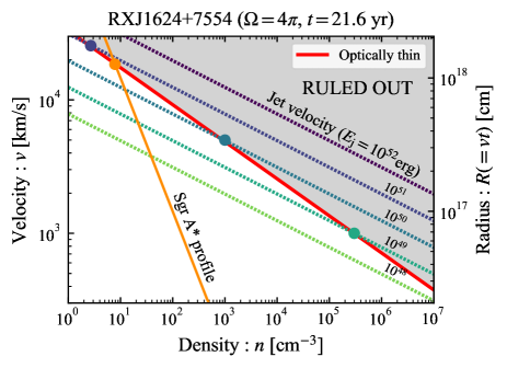
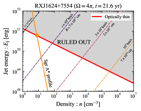
Figure 7: The same as Fig. 5 but for relativistic jets with different energies.

Figure 8: The density and jet energy ruled out by the no radio detection in RXJ1624+7554 at $t=21.6\,\rm yr$ for the case of a decelerated jet with $\Omega=4\pi$. Red line represents the boundary of the excluded region corresponding to the optically thin regime (Eq. 28). Each colored dash-dotted line shows the contour of each velocity and radius (see Eq. 26). The orange line denotes the energy of a jet expanding in Sgr A*-like profile. The intersection of this trajectory and ruled-out region gives the maximal jet energy for the Sgr A* profile (orange dot).

At late time an initially relativistic jet slows down and becomes Newtonian. Even if it is not completely spherical its emission would not be beamed. Energy conservation (Eq. 19), enables us to estimate the decelerated jet’s velocity at this phase

$$v \simeq\biggl{(}\frac{2E_{\rm j}}{\Omega m_{\rm{p}}nt^{3}}\biggl{)}^{1/5}\simeq 2.0\times 10^{5}{\,\rm km\,s^{-1}\,}E_{\rm j,51}^{1/5}n_{0}^{-1/5}t_{\rm yr}^{-3/5}\biggl{(}\frac{\Omega}{4\pi}\biggl{)}^{-1/5}\ ,$$ (26)

where we neglected the jet mass and approximated $R\simeq vt$. Depending on the initial properties of the jet and the external density profile the decelerating jet may remain non-spherical for a long time (Irwin et al., 2019, see also Fig. 10 in Appendix B). To take this into account we assume that the blast wave subtends a solid angle $\Omega$ into which all the jet’s energy is dissipated. The exact value of $\Omega$ depends on the details of the hydrodynamic evolution and the sideways propagation of the jet. However, as we show below, the resulting flux and limit on the energy depend weakly on $\Omega$. Hence, the exact determination of $\Omega$ is unimportant. The fact that the outflow remains jetted for a long time may imply that it also remains relativistic for a longer period, making it easier to hide a powerful jet that is pointing in a different directions even years after it was launched.

An estimate of the energy at which the jet becomes non-relativistic is given by setting $v\sim c$ in Eq. (26):

$$E_{\rm j,rel}\simeq\Omega m_{\rm{p}}nc^{5}t^{3}/2\simeq 8.0\times 10^{54}{\,\rm erg\,}n_{0}t_{\rm 10yr}^{3}\biggl{(}\frac{\Omega}{4\pi}\biggl{)}.$$ (27)

Hereafter, we change the normalization of time to $t_{10\rm yr}=t/10\,\rm yr$ corresponding to the observed values for the late-time upper-limits. For the Sgr A* profile, that we use below, the transition to Newtonian takes place at $t\simeq 0.34{\,\rm yr\,}E_{\rm j,52}^{1/2}(\Omega/4\pi)^{-1/2}$.

With Eqs. (16) and (26), the upper limits on the jet energy are given by

$$E_{\rm j,51}\lesssim\begin{cases}\big{(}0.60\big{)}_{p=2.5}\,\Big{[}\bar{\varepsilon}_{\rm{e,-1}}^{-1}\varepsilon_{\rm B,-2}^{-\frac{p+1}{4}}t_{\rm 10yr}^{\frac{3(p+1)}{10}}\nu_{\rm 3GHz}^{\frac{p-1}{2}}\\ \,\,\,\,\,\,d_{\rm L,27}^{2}F_{\rm 30\mu Jy}n_{0}^{-\frac{3(p+1)}{20}}\big{(}\frac{\Omega}{4\pi}\big{)}^{\frac{p+1}{10}}\Big{]}^{\frac{10}{p+11}}&\text{: $v<v_{\rm DN}$,}\\ \big{(}0.74\big{)}_{p=2.5}\,\Big{[}\bar{\varepsilon}_{\rm{e,-1}}^{1-p}\varepsilon_{\rm B,-2}^{-\frac{p+1}{4}}t_{\rm 10yr}^{\frac{3(5p-7)}{10}}\nu_{\rm 3GHz}^{\frac{p-1}{2}}\\ \,\,\,\,\,\,d_{\rm L,27}^{2}F_{\rm 30\mu Jy}n_{0}^{\frac{5p-19}{20}}\big{(}\frac{\Omega}{4\pi}\big{)}^{\frac{5p-7}{10}}\Big{]}^{\frac{10}{5p+3}}&\text{: $v>v_{\rm DN}$.}\end{cases}$$ (28)

Fig. 8 depicts trajectories of the decelerated jet’s velocity and the constraint from the radio upper-limit of RXJ1624+7554. We consider only the optically thin regime as at late time the observed frequency is typically above the SSA frequency. As the limit depends on the velocity, once we obtain a limit on the jet energy assuming either $v>$ (or $<$)$v_{\rm DN}$, we have to check using and Eq. (26) that the velocity satisfies the relevant condition. Clearly, the limits which we obtain assuming the system in a Newtonian phase, do not hold for extremely energetic jets that are observed early on and still relativistic at the observation epoch. The critical energy above which our assumption breaks down is given by Eq. (27). We miss such relativistic jets if they point away from our line of sight.

Fig. 8 depicts the excluded region in the density and jet energy space for the null detection in RXJ1624+7554. For each density, the maximal jet energy is given by Eq. (28). Assuming Sgr A* like density profile, $n\simeq 10{\,\rm cm^{-3}\,}(R/10^{18}\,\rm cm)^{-1}$ we can obtain a limit on the energy of the jets. Note that once a density profile is given we can calculate the radius and velocity more accurately than Eq. (26). However this does not change the results significantly (see Appendix B). The limits for Sgr A* profile are:

$$E_{\rm j,51} \lesssim\begin{cases}\big{(}0.21\big{)}_{p=2.5}\,\Big{[}\bar{\varepsilon}_{\rm{e,-1}}^{-1}\varepsilon_{\rm B,-2}^{-\frac{p+1}{4}}\nu_{\rm 3GHz}^{\frac{p-1}{2}}\\ \,\,\,\,\,\,t_{\rm 10yr}^{\frac{3(p+1)}{8}}d_{\rm L,27}^{2}F_{\rm 30\mu Jy}\big{(}\frac{\Omega}{4\pi}\big{)}^{\frac{p+1}{16}}\Big{]}^{\frac{16}{p+17}}&:v<v_{\rm DN}\ ,\\ \big{(}0.44\big{)}_{p=2.5}\,\Big{[}\bar{\varepsilon}_{\rm{e,-1}}^{1-p}\varepsilon_{\rm B,-2}^{-\frac{p+1}{4}}\nu_{\rm 3GHz}^{\frac{p-1}{2}}\\ \,\,\,\,\,\,t_{\rm 10yr}^{\frac{11p-13}{8}}d_{\rm L,27}^{2}F_{\rm 30\mu Jy}\big{(}\frac{\Omega}{4\pi}\big{)}^{\frac{3(3p-5)}{16}}\Big{]}^{\frac{16}{9p+1}}&:v>v_{\rm DN}\ .\\ \end{cases}$$ (29)

Note that the dependence on $\Omega$ is relatively weak, $\propto\Omega^{0.18}$ and $\Omega^{0.32}$ for $p=2.5$. As shown in Fig. 8, for RXJ1624+7554 with $F_{\nu}\lesssim 50{\,\mu\rm Jy}$ at $t\simeq 20{\,\rm yr}$ and Sgr A* like density profile, the energy is constrained to be $E_{\rm j}\lesssim 6\times 10^{50}\,\rm erg$. Importantly, with higher densities, as suggested in some radio-detected TDEs, the energy limit will be more severe.

For radio loud TDEs, we can calculate limits on the combinations of the jet energy, $E_{\rm j}$, and CNM density, $n$, as shown in Eq. (28). In particular, when the SSA frequency is identified as a spectral peak $\nu_{\rm p}$, we can directly estimate the energy corresponding to the minimal velocities $v_{\rm eq}$ in Eq. (17). This energy is given by plunging $v_{\rm eq}$ and $n_{\rm eq}$ into Eq. (26):

$$E_{\rm j,eq}\simeq\begin{cases}\big{(}4.2\times 10^{47}{\,\rm erg}\big{)}_{p=2.5}\,\Big{[}\bar{\varepsilon}_{\rm{e,-1}}^{-11}\varepsilon_{\rm B,-2}^{-2(p+1)}\\ \,\,\,F_{30\mu\rm Jy}^{3p+14}d_{\rm L,27}^{2(3p+14)}\big{(}\frac{\Omega}{4\pi}\big{)}^{-(p+1)}\Big{]}^{\frac{1}{2p+13}}\nu_{\rm p,3GHz}^{-1}&:v<v_{\rm DN},\\ \big{(}1.0\times 10^{49}{\,\rm erg}\big{)}_{p=2.5}\,\Big{[}\bar{\varepsilon}_{\rm{e,-1}}^{11(1-p)}\varepsilon_{\rm B,-2}^{2(1-2p)}\nu_{\rm p,3GHz}^{18p-53}\\ \,\,\,t_{\rm 10yr}^{22(p-2)}F_{30\mu\rm Jy}^{5(6-p)}d_{\rm L,27}^{10(6-p)}\big{(}\frac{\Omega}{4\pi}\big{)}^{9p-21}\Big{]}^{\frac{1}{4p+9}}&:v>v_{\rm DN}.\end{cases}$$ (30)

Based on the radio observations, the jet energy of Sw1644 has been estimated by many authors (Berger et al., 2012; Metzger et al., 2012; Zauderer et al., 2013; Barniol Duran & Piran, 2013; Mimica et al., 2015; Eftekhari et al., 2018; De Colle & Lu, 2020; Cendes et al., 2021b). At late time $\gtrsim 300\,\rm days$, the outflow decelerates to the Newtonian phase and our method can be applied. By using Eq. (30) we estimate the jet energy $E_{\rm j,eq}\sim 10^{52}\,\rm erg$, which is consistent with the other estimates at this stage (Barniol Duran & Piran, 2013; De Colle & Lu, 2020; Cendes et al., 2021b).

For TDEs with radio upper-limits, we calculate the upper limits on the jet energy assuming an Sgr A* like profile (Eq. 29). Fig. 9 depicts the allowed jet energy for each upper limit (see also Table 1). At $t\gtrsim$ a few years we can assume that a jet with reasonable energy became Newtonian. We find that typical upper limits are in the range $10^{50-52}\,\rm erg$ for events with late observations. Among those, an energetic jet similar to Sw1644 is excluded in events observed more than a few years after the TDE, regardless of the opening angle. For events with early observations we obtain limits in the range $10^{47-49}\,\rm erg$. However, in these cases we cannot rule out much more energetic jets that point away from us and are still in the relativistic regime (Eq. 27). Note that these values are for Sgr A* like density distribution. The limits will be stronger if the surrounding density is larger, for example like the one inferred for ASASSN-14li (Alexander et al., 2016; Krolik et al., 2016).

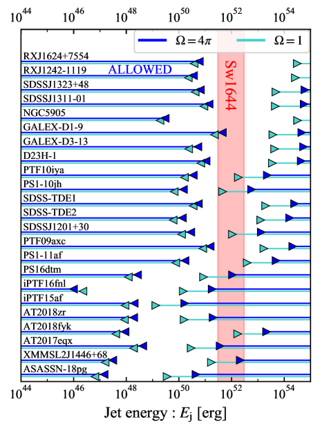
Figure 9: Jet energy allowed by radio null detection assuming a CNM density similar to the Sgr A* profile. At the time of observations the outflow is assumed to have a solid angle $\Omega=4\pi$ (blue) or $1$ (turquoise - conservatively corresponding to the half-opening angle of $\simeq 0.57{\,\rm rad}\simeq 33^{\circ}$, see Fig. 10). Limits obtained more than a few years after the TDE rule out jets with energy $E_{\rm j}\sim 10^{52}\,\rm erg$ similar to Sw1644. For limits at early time ($\lesssim 0.1\,\rm yr$), we cannot reject jets with $E_{\rm j}\gtrsim 10^{51-52}$ erg (Eq. 27) because such jets are still relativistic and may beam their radiation away from our line of sight.

van Velzen et al. (2013) constrained the jet energy for several TDEs with radio upper-limits to be $E_{\rm j}<10^{52}\,\rm erg$ by converting the on-axis light curve for Sw1644 (Metzger et al., 2012; Berger et al., 2012) to off-axis ones. But this estimate ignored the sideways expansion and is invalid for the late phase when the observations were carried out. Generozov et al. (2017) derived upper limits on the jet energy based on numerical simulation (Mimica et al., 2015). Remarkably, their constraints $E_{\rm j}\lesssim 10^{53}\,\rm erg$ are $\simeq 20-60$ times weaker than ours for the same parameter values. We find that the scaling of their light curves are consistent with ours but the peak time and peak luminosity (when the jet becomes optically thin, $\nu\simeq{\nu}_{\rm{a}}$) are about 4 and 10 times shorter and dimmer than our estimates, respectively. In Appendix B we provide a specific detailed calculation for the limit on RXJ1624+7554 as an example so that our method can be directly compared to theirs. In this case our upper limit of $E_{\rm j}\lesssim 7\times 10^{50}$ erg is about 30 times smaller than the one obtained by Generozov et al. (2017). Comparison of our hydrodynamics simulations (see Fig. 10) to theirs shows consistency, suggesting that the difference originates in the calculations of the synchrotron emission. In spite of some joint efforts we could not identify the origin of this discrepancy. Note that Mimica et al. (2015) find a jet energy of $\simeq 5\times 10^{53}\,\rm erg$ for Sw1644, which is larger by a similar factor than our and other estimates (Barniol Duran & Piran, 2013; De Colle & Lu, 2020; Cendes et al., 2021b) of $E_{\rm j}\sim 10^{52}\,\rm erg$.

5 Summary

We analyzed the radio observations and upper limits of TDEs within a model in which the radio emission arises due to the interaction of an outflow with the CNM leading to synchrotron emission from the shocked material. Within this model we constrained the outflow properties and the CNM density in the galactic nuclear regions. Our analysis systematically constrains the combination $v\Omega^{a}$, where $a\simeq 0.5$. Depending on the details of the parameters of the outflow velocity $v$ and the solid angle $\Omega$, it also constrains the CNM density $n$ at the observation epoch. When the spectral peak is available, our method is similar to the equipartition method (Chevalier, 1998; Barniol Duran et al., 2013). However, we obtained significant limits also in cases in which only a single frequency is observed or in which there are just upper limits. In particular, we found that a given detection implies a minimal outflow velocity (Eq. 17), that depends only on the solid angle $\Omega$ and on the assumed (or measured) value of the electrons distribution index $p$. We considered four outflow models: disk wind, unbound debris, and Newtonian jets, corresponding to spherical, wedge and conical geometries, and relativistic jets.

Our calculations considered the deep-Newtonian regime ($v<v_{\rm DN}\simeq 6\times 10^{4}\,\rm km\,s^{-1}$) in which only a small fraction $\sim(v/v_{\rm DN})^{2}\simeq 0.01-0.03$ of the total number of electrons is relativistic and contributes to synchrotron emission. This implies that our estimates of the CNM density and swept-up CNM mass are $\sim 30-100$ times larger than those found in the previous works based on the equipartition method (Alexander et al., 2016; Krolik et al., 2016; Anderson et al., 2020; Stein et al., 2021; Cendes et al., 2021a) that did not take this effect into account.

Isotropic disk winds with an initial velocity $v_{\rm in}\simeq 10^{4}\,\rm km\,s^{-1}$ can easily produce the observed radio flares as discussed in previous analysis (Alexander et al., 2016; Anderson et al., 2020; Stein et al., 2021; Cendes et al., 2021a). For radio-detected TDEs, in particular for events with a measured spectral peak, we found that the wind does not decelerate significantly. This suggests that the wind’s mass should be larger than the swept-up CNM mass $M_{\rm ej}\gtrsim M(R)\simeq 0.01-0.1\,\mathrm{M}_{\odot}$. Therefore, current observations do not necessarily require a massive disk wind as suggested by the reprocessed model $M_{\rm ej}\simeq 0.5\mathrm{M}_{\odot}$ (Metzger & Stone, 2016). Assuming the same typical velocity $v_{\rm in}=10^{4}\,\rm km\,s^{-1}$, we found that some of radio null detection require CNM densities significantly smaller than those required in radio-detected TDEs. This means that not all TDEs drive sufficiently fast isotropic outflows or the density profiles of galactic nuclear regions vary among galaxies. For the TDEs with upper limit determined at ten or more years after the event the implied density upper-limits become comparable to the CNM density around Sgr A*.

We found that unbound debris with mass $\simeq 0.5\,\mathrm{M}_{\odot}$, velocity $\sim 10^{4}\,\rm km\,s^{-1}$, and (bow shock’s) solid angle $\Omega\simeq 0.1$, cannot produce the detectable radio flare due to its too small solid angle. While this limit is slightly relaxed if we take into account that the shock velocity is larger than the fluid velocity, this is not sufficient to fully resolve the discrepancy. However, as suggested by Yalinewich et al. (2019), higher velocities and larger solid angles ($\Omega\sim 1$) can arise when the stellar pericenter is well below the tidal radius (deep penetration). In such cases the debris can produce a detectable radio flare (Krolik et al., 2016). Rarity of such deep-penetration events may explain why radio detection is not common.

We also considered conical outflows (Newtonian jets) and found that those could be the observed radio sources. Such jets can be realized, for instance, by a disk wind with an angular structure. Lacking a specific model for the formation of such jets and no definite predictions on their properties, one can always find model parameters that fit the observations. We can only derive scaling relations between the minimal velocity and the required density for the solid angle $\Omega<4\pi$ (assuming the jet mass is larger than the swept-up CNM mass). Both velocity and density increase roughly $\propto\Omega^{-0.5}$.

Radio upper-limits also constrain the energy of relativistic jets accompanying TDEs. We can safely reject jets as energetic as Sw1644, $E_{\rm j}\sim 10^{52}\,\rm erg$ for TDEs with upper limits at $t\gtrsim$ a few years. Note however, that it is impossible to exclude extremely energetic jets with energies $>10^{53}\,\rm erg$ that have not decelerated yet to the Newtonian phase. Future late observations will however, rule out or identify such jets. For upper limits at $t\lesssim 0.01-0.1\,\rm yr$, we have very tight constraints on the existence of jets with energy $E_{\rm j}\lesssim 10^{47-49}\,\rm erg$ while we cannot exclude jets with $E_{\rm j}\gtrsim 10^{51}\,\rm erg$. These jets are still relativistic and hence beamed away from us at the time of observations. They will be ruled out if no radio signals are detected a few years after the discovery. Therefore we encourage continuous radio monitoring to search for energetic off-axis TDE jets.

Radio-detected TDEs have been suggested as a tool to explore the CNM density profiles of distant galactic centers. So far we could explore this profile only for the Milky Way. However, our results show that without knowing the outflow’s geometry $\Omega$ and the velocity $v$ (or more precisely the velocity distribution $M_{\rm ej}(>v)$), it is in fact impossible to determine the exact value of the CNM profile from the radio observations alone. With reasonable assumptions we can estimate the profile’s radial behavior but not the exact normalization. Within the models that we considered, the CNM density of radio-detected events is $\gtrsim 10^{2}$ times larger than that of Sgr A* profile, and its slope is typically $n(R)\propto R^{-3}$.

The total luminosity from synchrotron emission is determined by the peak of $\nu F_{\nu}$. For slow cooling, which is relevant in all cases considered, this peak corresponds to the cooling frequency (e.g. Sari et al., 1998):

$$\nu_{\rm c} =\frac{18\pi m_{\rm{e}}ce}{\sigma_{\rm T}^{2}B^{3}t^{2}}\simeq 6.2\times 10^{18}{\,\rm Hz\,}\varepsilon_{\rm B,-2}^{-3/2}n_{0}^{-3/2}v_{9}^{-3}t_{\rm yr}^{-2}\ .$$ (31)

As we have seen, for radio-detected events the required density is $n\sim 10^{5}\,\rm cm^{-3}$ implying $\nu_{\rm c}\simeq 2.0\times 10^{11}\,\rm Hz$. By using the observed luminosity $\nu L_{\nu}\sim 10^{38}\,\rm erg\,s^{-1}$ at $5\,\rm GHz$ and noting that luminosity scales $\nu L_{\nu}\propto\nu^{(3-p)/2}$, we estimate the total luminosity

$$L\sim\nu_{\rm c}L_{\nu_{\rm c}}\simeq\big{(}2\times 10^{38}{\,\rm erg\,s^{-1}}\big{)}_{p=2.5}\,\nu_{\rm c,11}^{\frac{3-p}{2}}\ .$$ (32)

For reasonable parameters, the peak luminosity is less than $10^{40}\,\rm erg\,s^{-1}$. The total emitted energy $\sim tL\simeq 10^{47}\,\rm erg$ is much smaller than the kinetic energy $M_{\rm ej}v^{2}/2\sim 10^{50}{\,\rm erg\,}M_{\rm ej,-1}v_{9}^{2}$, for the sources considered here. This implies that, unlike claims in the literature (e.g. Cendes et al., 2021a; Stein et al., 2021), to produce the observed emission there is no need to consider additional energy-injection into the outflow (Matsumoto et al. in prep).

To conclude we have shown here the importance of late radio followup of TDEs. Somewhat surprisingly these observations whose schedule can be flexible are very significant. Upper limits taken 20 years or more after the event provide interesting limits on properties of the outflow, the nature of the TDE, and on the density structure surrounding the supermassive BH.

data availability

The data underlying this article will be shared on reasonable request to the corresponding author.

Appendix A Formulae for a general power-law index of electron distribution

We present the formulae for general $p$. The equations for SSA frequency and fluxes corresponding to Eqs. (8), (10), (11) and (12) are given by

$${\nu}_{\rm{a}} \simeq\begin{cases}7.2\times 10^{3}\big{[}8.2\times 10^{7}(p-1)\,3^{\frac{p+1}{2}}\big{]}^{\frac{2}{p+4}}{\,\rm Hz\,}\\ \,\,\,\,\,\,\bar{\varepsilon}_{\rm{e,-1}}^{\frac{2}{p+4}}\varepsilon_{\rm B,-2}^{\frac{p+2}{2(p+4)}}n_{0}^{\frac{p+6}{2(p+4)}}v_{9}^{\frac{p+6}{p+4}}R_{17}^{\frac{2}{p+4}}&:\,v<v_{\rm DN},\\ 4.7\big{[}3.0\times 10^{17}(p-1)\,3^{\frac{p+1}{2}}\big{]}^{\frac{2}{p+4}}{\,\rm Hz\,}\\ \,\,\,\,\,\,\bar{\varepsilon}_{\rm{e,-1}}^{\frac{2(p-1)}{p+4}}\varepsilon_{\rm B,-2}^{\frac{p+2}{2(p+4)}}n_{0}^{\frac{p+6}{2(p+4)}}v_{9}^{\frac{5p-2}{p+4}}R_{17}^{\frac{2}{p+4}}&:\,v_{\rm DN}<v.\end{cases}$$ (33)

$$F_{{\nu}_{\rm{a}}} \simeq\begin{cases}0.62\big{[}8.2\times 10^{7}(p-1)\,3^{\frac{p+1}{2}}\big{]}^{\frac{1-p}{p+4}}{\,\rm\mu Jy\,}\bar{\varepsilon}_{\rm{e,-1}}^{\frac{5}{p+4}}\\ \,\,\,\varepsilon_{\rm B,-2}^{\frac{2p+3}{2(p+4)}}n_{0}^{\frac{2p+13}{2(p+4)}}v_{9}^{\frac{2p+13}{p+4}}R_{17}^{\frac{2p+13}{p+4}}\big{(}\frac{\Omega}{4\pi}\big{)}d_{\rm L,27}^{-2}&:\,v<v_{\rm DN},\\ 25\big{[}3.0\times 10^{17}(p-1)\,3^{\frac{p+1}{2}}\big{]}^{\frac{1-p}{p+4}}{\,\rm\mu Jy\,}\bar{\varepsilon}_{\rm{e,-1}}^{\frac{5(p-1)}{p+4}}\\ \,\,\,\varepsilon_{\rm B,-2}^{\frac{2p+3}{2(p+4)}}n_{0}^{\frac{2p+13}{2(p+4)}}v_{9}^{\frac{12p-7}{p+4}}R_{17}^{\frac{2p+13}{p+4}}\big{(}\frac{\Omega}{4\pi}\big{)}d_{\rm L,27}^{-2}&:\,v_{\rm DN}<v,\end{cases}$$ (34)

$$F_{\nu>{\nu}_{\rm{a}}} \simeq\begin{cases}0.62\big{[}4.1\times 10^{5}\big{]}^{\frac{1-p}{2}}{\,\rm\mu Jy\,}\bar{\varepsilon}_{\rm{e,-1}}\\ \,\,\,\varepsilon_{\rm B,-2}^{\frac{p+1}{4}}n_{0}^{\frac{p+5}{4}}v_{9}^{\frac{p+5}{2}}R_{17}^{3}\big{(}\frac{\Omega}{4\pi}\big{)}\nu_{\rm 3GHz}^{\frac{1-p}{2}}d_{\rm L,27}^{-2}&:\,v<v_{\rm DN},\\ 25\big{[}6.4\times 10^{8}\big{]}^{\frac{1-p}{2}}{\,\rm\mu Jy\,}\bar{\varepsilon}_{\rm{e,-1}}^{p-1}\\ \,\,\,\varepsilon_{\rm B,-2}^{\frac{p+1}{4}}n_{0}^{\frac{p+5}{4}}v_{9}^{\frac{5p-3}{2}}R_{17}^{3}\big{(}\frac{\Omega}{4\pi}\big{)}\nu_{\rm GHz}^{\frac{1-p}{2}}d_{\rm L,27}^{-2}&:\,v_{\rm DN}<v,\end{cases}$$ (35)

$$F_{\nu<{\nu}_{\rm{a}}} \simeq\frac{8.4\times 10^{4}}{(p-1)3^{\frac{p+1}{2}}}{\,\rm\mu Jy\,}\varepsilon_{\rm B,-2}^{-1/4}$$

$$\,\,\,\,\,\,\,\,\,\,\,\,n_{0}^{-1/4}v_{9}^{-1/2}R_{17}^{2}\biggl{(}\frac{\Omega}{4\pi}\biggl{)}\nu_{\rm 3GHz}^{5/2}d_{\rm L,27}^{-2},$$ (36)

respectively. Constraints on the combinations of the density, velocity, and solid angle, are given by

$$n_{0}^{\frac{p+5}{4}}v_{9}^{\frac{p+11}{2}}\Omega\lesssim 1.9\times 10^{4}\big{[}4.1\times 10^{5}\big{]}^{\frac{p-1}{2}}$$

$$\,\,\,\,\,\,\bar{\varepsilon}_{\rm{e,-1}}^{-1}\varepsilon_{\rm B,-2}^{-\frac{p+1}{4}}t_{\rm yr}^{-3}\nu_{\rm 3GHz}^{\frac{p-1}{2}}d_{\rm L,27}^{2}F_{\rm 30\mu Jy},$$ (37)

for optically thin and the deep-Newtonian phase (Eq. 13),

$$n_{0}^{\frac{p+5}{4}}v_{9}^{\frac{5p+3}{2}}\Omega\lesssim 500\big{[}6.4\times 10^{8}\big{]}^{\frac{p-1}{2}}$$

$$\,\,\,\,\,\,\bar{\varepsilon}_{\rm{e,-1}}^{1-p}\varepsilon_{\rm B,-2}^{-\frac{p+1}{4}}t_{\rm yr}^{-3}\nu_{\rm 3GHz}^{\frac{p-1}{2}}d_{\rm L,27}^{2}F_{\rm 30\mu Jy},$$ (38)

for optically thin and $v>v_{\rm DN}$ case (Eq. 14), and

$$n_{0}^{-1/4}v_{9}^{3/2}\Omega\lesssim 4.5\times 10^{-3}(p-1)3^{\frac{p+1}{2}}\varepsilon_{\rm B,-2}^{1/4}t_{\rm yr}^{-2}\nu_{\rm 3GHz}^{-5/2}d_{\rm L,27}^{2}F_{\rm 30\mu Jy}.$$ (39)

for optically thick case (Eq. 15). The limit on velocity corresponding to Eq. (16) is

$$v_{9}\lesssim\begin{cases}\Big{[}1.9\times 10^{4}\big{(}4.1\times 10^{5}\big{)}^{\frac{p-1}{2}}\bar{\varepsilon}_{\rm{e,-1}}^{-1}\varepsilon_{\rm B,-1}^{-\frac{p+1}{4}}\\ \,\,\,t_{\rm yr}^{-3}\nu_{\rm 3GHz}^{\frac{p-1}{2}}d_{\rm L,27}^{2}F_{\rm 30\mu Jy}n_{0}^{-\frac{p+5}{4}}\Omega^{-1}\Big{]}^{\frac{2}{p+11}}&:{\rm thin\,}(v<v_{\rm DN}),\\ \Big{[}500\big{(}6.4\times 10^{8}\big{)}^{\frac{p-1}{2}}\bar{\varepsilon}_{\rm{e,-1}}^{1-p}\varepsilon_{\rm B,-2}^{-\frac{p+1}{4}}\\ \,\,\,t_{\rm yr}^{-3}\nu_{\rm 3GHz}^{\frac{p-1}{2}}d_{\rm L,27}^{2}F_{\rm 30\mu Jy}n_{0}^{-\frac{p+5}{4}}\Omega^{-1}\Big{]}^{\frac{2}{5p+3}}&:{\rm thin\,}(v>v_{\rm DN}),\\ 2.7\times 10^{-2}(p-1)^{2/3}3^{\frac{p+1}{3}}\varepsilon_{\rm B,-2}^{1/6}\\ \,\,\,t_{\rm yr}^{-4/3}\nu_{\rm 3GHz}^{-5/3}d_{\rm L,27}^{4/3}F_{\rm 30\mu Jy}^{2/3}n_{0}^{1/6}\Omega^{2/3}&:{\rm thick}.\end{cases}$$ (40)

The minimal velocities and corresponding densities are given by

$$v_{\rm eq,9} \simeq\begin{cases}\big{[}1.9\times 10^{4}(4.1\times 10^{5})^{\frac{p-1}{2}}\big{]}^{\frac{1}{2p+13}}\\ \,\,\,\big{[}4.5\times 10^{-3}(p-1)3^{\frac{p+1}{2}}\big{]}^{\frac{p+5}{2p+13}}\bar{\varepsilon}_{\rm{e,-1}}^{-\frac{1}{2p+13}}\\ \,\,\,\,\,\,\varepsilon_{\rm B,-2}^{\frac{1}{2p+13}}t_{\rm yr}^{-1}\nu_{\rm 3GHz}^{-1}d_{\rm L,27}^{\frac{2(p+6)}{2p+13}}F_{\rm 30\mu Jy}^{\frac{p+6}{2p+13}}\Omega^{-\frac{p+6}{2p+13}}&:v<v_{\rm DN},\\ \big{[}500(6.4\times 10^{8})^{\frac{p-1}{2}}\big{]}^{\frac{1}{4p+9}}\\ \,\,\,\big{[}4.5\times 10^{-3}(p-1)3^{\frac{p+1}{2}}\big{]}^{\frac{p+5}{4p+9}}\bar{\varepsilon}_{\rm{e,-1}}^{\frac{1-p}{4p+9}}\\ \,\,\,\,\,\,\varepsilon_{\rm B,-2}^{\frac{1}{4p+9}}t_{\rm yr}^{-\frac{2p+13}{4p+9}}\nu_{\rm 3GHz}^{-\frac{2p+13}{4p+9}}d_{\rm L,27}^{\frac{2(p+6)}{4p+9}}F_{\rm 30\mu Jy}^{\frac{p+6}{4p+9}}\Omega^{-\frac{p+6}{4p+9}}&:v>v_{\rm DN},\end{cases}$$ (41)

$$n_{\rm eq,0} \simeq\begin{cases}\big{[}1.9\times 10^{4}(4.1\times 10^{5})^{\frac{p-1}{2}}\big{]}^{\frac{6}{2p+13}}\\ \,\,\,\big{[}4.5\times 10^{-3}(p-1)3^{\frac{p+1}{2}}\big{]}^{-\frac{2(p+11)}{2p+13}}\bar{\varepsilon}_{\rm{e,-1}}^{-\frac{6}{2p+13}}\\ \,\,\,\,\,\,\varepsilon_{\rm B,-2}^{-\frac{2p+7}{2p+13}}t_{\rm yr}^{2}\nu_{\rm 3GHz}^{4}d_{\rm L,27}^{-\frac{4(p+8)}{2p+13}}F_{\rm 30\mu Jy}^{-\frac{2(p+8)}{2p+13}}\Omega^{\frac{2(p+8)}{2p+13}}&:v<v_{\rm DN},\\ \big{[}500(6.4\times 10^{8})^{\frac{p-1}{2}}\big{]}^{\frac{6}{4p+9}}\\ \,\,\,\big{[}4.5\times 10^{-3}(p-1)3^{\frac{p+1}{2}}\big{]}^{-\frac{2(5p+3)}{4p+9}}\bar{\varepsilon}_{\rm{e,-1}}^{\frac{6(1-p)}{4p+9}}\\ \,\,\,\,\,\,\varepsilon_{\rm B,-2}^{-\frac{4p+3}{4p+9}}t_{\rm yr}^{\frac{2(10p-3)}{4p+9}}\nu_{\rm 3GHz}^{\frac{4(7p+3)}{4p+9}}d_{\rm L,27}^{-\frac{20p}{4p+9}}F_{\rm 30\mu Jy}^{-\frac{10p}{4p+9}}\Omega^{\frac{10p}{4p+9}}&:v>v_{\rm DN}.\\ \end{cases}$$ (42)

corresponding to Eqs. (17) and (18), respectively.

Constraints on the jet energy for each case (Eq. 28) and minimal jet energies (Eq. 30) are given by

$$E_{\rm j,51}\lesssim\begin{cases}\Big{[}1.8\times 10^{-7}(150)^{p}\bar{\varepsilon}_{\rm{e,-1}}^{-1}\varepsilon_{\rm B,-2}^{-\frac{p+1}{4}}t_{\rm yr}^{\frac{3(p+1)}{10}}\\ \,\,\,\nu_{\rm 3GHz}^{\frac{p-1}{2}}d_{\rm L,27}^{2}F_{\rm 30\mu Jy}n_{0}^{-\frac{3(p+1)}{20}}\big{(}\frac{\Omega}{4\pi}\big{)}^{\frac{p+1}{10}}\Big{]}^{\frac{10}{p+11}}&\text{: $v<v_{\rm DN}$,}\\ \Big{[}1.8\times 10^{-5}(15)^{p}\bar{\varepsilon}_{\rm{e,-1}}^{1-p}\varepsilon_{\rm B,-2}^{-\frac{p+1}{4}}t_{\rm yr}^{\frac{3(5p-7)}{10}}\\ \,\,\,\nu_{\rm 3GHz}^{\frac{p-1}{2}}d_{\rm L,27}^{2}F_{\rm 30\mu Jy}n_{0}^{\frac{5p-19}{20}}\big{(}\frac{\Omega}{4\pi}\big{)}^{\frac{5p-7}{10}}\Big{]}^{\frac{10}{5p+3}}&\text{: $v>v_{\rm DN}$,}\\ \end{cases}$$ (43)

$$E_{\rm j,eq}\simeq\begin{cases}1.1\times 10^{44}{\,\rm erg\,}\Big{[}5.8(9.0\times 10^{20})^{p}\\ \,\,\,(5.2)^{p^{2}}(p-1)^{3(p+1)}\bar{\varepsilon}_{\rm{e,-1}}^{-11}\varepsilon_{\rm B,-2}^{-2(p+1)}\\ \,\,\,\,\,\,d_{\rm L,27}^{2(3p+14)}F_{30\mu\rm Jy}^{3p+14}\big{(}\frac{\Omega}{4\pi}\big{)}^{-(p+1)}\Big{]}^{\frac{1}{2p+13}}\nu_{\rm 3GHz}^{-1}&:v<v_{\rm DN},\\ 3.3\times 10^{44}{\,\rm erg\,}\Big{[}1.8\times 10^{-92}(9.8\times 10^{68})^{p}\\ \,\,\,(0.064)^{p^{2}}(p-1)^{19-5p}\bar{\varepsilon}_{\rm{e,-1}}^{11(1-p)}\varepsilon_{\rm B,-2}^{2(1-2p)}\\ \,\,\,\,\,\,t_{\rm yr}^{22(p-2)}\nu_{\rm 3GHz}^{18p-53}d_{\rm L,27}^{10(6-p)}F_{30\mu\rm Jy}^{5(6-p)}\big{(}\frac{\Omega}{4\pi}\big{)}^{9p-21}\Big{]}^{\frac{1}{4p+9}}&:v>v_{\rm DN}.\\ \end{cases}$$ (44)

For Sgr A* like density profile, the jet energy is constrained by

$$E_{\rm j,51} \lesssim\begin{cases}\Big{[}1.1\times 10^{-7}(86)^{p}\bar{\varepsilon}_{\rm{e,-1}}^{-1}\varepsilon_{\rm B,-2}^{-\frac{p+1}{4}}t_{\rm yr}^{\frac{3(p+1)}{8}}\\ \,\,\,\,\,\,\nu_{\rm 3GHz}^{\frac{p-1}{2}}d_{\rm L,27}^{2}F_{\rm 30\mu Jy}\big{(}\frac{\Omega}{4\pi}\big{)}^{\frac{p+1}{16}}\Big{]}^{\frac{16}{p+17}}&:v<v_{\rm DN},\\ \Big{[}6.6\times 10^{-7}(35)^{p}\bar{\varepsilon}_{\rm{e,-1}}^{1-p}\varepsilon_{\rm B,-2}^{-\frac{p+1}{4}}t_{\rm yr}^{\frac{11p-13}{8}}\\ \,\,\,\,\,\,\nu_{\rm 3GHz}^{\frac{p-1}{2}}d_{\rm L,27}^{2}F_{\rm 30\mu Jy}\big{(}\frac{\Omega}{4\pi}\big{)}^{\frac{3(3p-5)}{16}}\Big{]}^{\frac{16}{9p+1}}&:v>v_{\rm DN}.\\ \end{cases}$$ (45)

Appendix B More precise estimation of the jet energy

We present a detailed calculation of the upper limit on the jet energy for RXJ1624+7554. The radio upper-limit is $F_{\nu}=51\,\rm\mu Jy$ at $\nu=3\,\rm GHz$ with $d_{\rm L}=270\,\rm Mpc$ and $t=21.7\,\rm yr$ (see Table 1). We consider a Milky-Way like density profile, $n(R)=\tilde{n}(R/\tilde{R})^{-k}$ with $\tilde{n}=10\,\rm cm^{-3}$, $\tilde{R}=10^{18}\,\rm cm$, and $k=1$. In the Newtonian phase, the jet energy is given by

$$E_{j}=\Omega m_{\rm{p}}\frac{v^{2}}{2}\int_{0}^{R}r^{2}n(r)dr=\frac{\Omega m_{\rm{p}}}{2(3-k)}\tilde{n}\tilde{R}^{k}v^{2}R^{3-k}.$$ (46)

Note that in this section we take into account the numerical factors that are ignored in §4. Using $R\propto t^{l}$ with $l=2/(5-k)=0.5$, we obtain the relation between the velocity and radius as $v=\frac{dR}{dt}=lR/t$. Substituting this into Eq. (46) and setting $v=c$, we obtain the timescale at which the jet becomes Newtonian

$$t_{\rm NR} =\biggl{(}\frac{2(3-k)l^{3-k}E_{\rm j}}{\Omega m_{\rm{p}}c^{5-k}\tilde{n}\tilde{R}^{k}}\biggl{)}^{\frac{1}{3-k}}\simeq 7.7\times 10^{-2}{\,\rm yr\,}E_{\rm j,51}^{1/2}\biggl{(}\frac{\Omega}{4\pi}\biggl{)}^{-1/2}.$$ (47)

The jet is Newtonian at the observation time as long as $E_{\rm j}\lesssim E_{\rm j,rel}\simeq 8\times 10^{55}\,\rm erg\,(\Omega/4\pi)$. The time evolution of the jet velocity and radius for $t>t_{\rm NR}$ are given by

$$v =c\biggl{(}\frac{t}{t_{\rm NR}}\biggl{)}^{l-1}\simeq 18000{\,\rm km\,s^{-1}\,}E_{\rm j,51}^{1/4}\biggl{(}\frac{t}{21.7{\,\rm yr}}\biggl{)}^{-1/2}\biggl{(}\frac{\Omega}{4\pi}\biggl{)}^{-1/4},$$ (48)

$$R =\frac{ct_{\rm NR}}{l}\biggl{(}\frac{t}{t_{\rm NR}}\biggl{)}^{l}\simeq 2.5\times 10^{18}{\,\rm cm\,}E_{\rm j,51}^{1/4}\biggl{(}\frac{t}{21.7{\,\rm yr}}\biggl{)}^{1/2}\biggl{(}\frac{\Omega}{4\pi}\biggl{)}^{-1/4}.$$ (49)

These estimates are reasonably consistent with the 2D jet simulation shown in Fig. 10 but also with the 1D simulation of Mimica et al. (2015). By using these equations with Eq. (35), we derive the flux at the optically thin regime:

$$F_{\nu} \simeq\begin{cases}79{\,\rm\mu Jy\,}\varepsilon_{\rm e,-1}\big{(}\frac{\varepsilon_{\rm B}}{0.002}\big{)}^{0.83}E_{\rm j,51}^{1.21}\big{(}\frac{t}{21.7\,\rm yr}\big{)}^{-1.24}\\ \,\,\,\,\,\,\nu_{\rm 3GHz}^{-0.65}\big{(}\frac{d_{\rm L}}{270\,\rm Mpc}\big{)}^{-2}\big{(}\frac{\Omega}{4\pi}\big{)}^{-0.21}&:v<v_{\rm DN},\\ 36{\,\rm\mu Jy\,}\varepsilon_{\rm e,-1}^{1.3}\big{(}\frac{\varepsilon_{\rm B}}{0.002}\big{)}^{0.83}E_{\rm j,51}^{1.36}\big{(}\frac{t}{21.7\,\rm yr}\big{)}^{-1.54}\\ \,\,\,\,\,\,\nu_{\rm 3GHz}^{-0.65}\big{(}\frac{d_{\rm L}}{270\,\rm Mpc}\big{)}^{-2}\big{(}\frac{\Omega}{4\pi}\big{)}^{-0.36}&:v>v_{\rm DN},\\ \end{cases}$$ (50)

where we adopt the same micro-physics parameters as Generozov et al. (2017) ($\varepsilon_{\rm e}=0.1$, $\varepsilon_{\rm B}=0.002$, and $p=2.3$). We find that for RXJ1624+7554, the deep-Newtonian phase ($v<v_{\rm DN}$) is relevant and we obtain a limit of $E_{\rm j}\lesssim 7.0\times 10^{50}\,\rm erg$, which is $\simeq 30$ times smaller than the one of Generozov et al. (2017). It should be noted that Generozov et al. (2017) did not consider the deep-Newtonian phase and calculated the limit for the normal phase ($v>v_{\rm DN}$). However, this does not change the limit on jet significantly ($E_{\rm j}\lesssim 1.3\times 10^{51}\,\rm erg$).

Figure 10: 2D hydrodynamics simulation of a relativistic jet carried out by Matteo Pais using PLUTO (Mignone et al., 2007). The jet is injected with energy $E_{\rm j}=10^{53}\,\rm erg$ and half-opening angle $\theta=20^{\circ}$ into a Sgr A* like CNM, $n(R)=10{\,\rm cm^{-3}\,}(R/10^{18}\,{\rm cm})^{-1}$. The velocity ($\beta\equiv{v/c}$) distribution at $t=21.7{\,\rm yr}$ after the launch (the same as the observation of RXJ1624+7554) shows that while the system is almost Newtonian (the highest $\beta$ values are around 0.5) the jet is not spherical yet. The resulting cocoon has a bipolar shape with an opening angle of $\theta\simeq 30^{\circ}$.

Appendix C Constraint for each event

We present our complete results on radio upper-limits (Table 1) and radio-detected events (Table 2).

Table 1: Constraints imposed by radio upper-limits for the cases of isotropic disk wind, unbound debris, and relativistic jet. For the former two cases, we show the minimal velocity $v_{\rm eq}$, corresponding density $n_{\rm eq}$, limiting velocity in the optically thin regime $v_{-}$, and the corresponding density upper-limit $n_{-}$. For relativistic jet, the upper limit $E_{\rm j}$ is relevant up to the energy $E_{\rm j,rel}$.

Event (Ref)	Redshift	Time	Freq.	Flux	Disk wind ($\Omega=4\pi$)				Unbound debris ($\Omega=0.1$)				Relativistic jet ($\Omega=4\pi$)
	$z$	$t$	$\nu$	$F_{\nu}$	$v_{\rm eq}$	$n_{\rm eq}$	$v_{-}$	$n_{-}$	$v_{\rm eq}$	$n_{\rm eq}$	$v_{-}$	$n_{-}$	$E_{\rm j}$	$E_{\rm j,rel}$
		[yr]	[GHz]	[$\mu$Jy]	[km/s]	[$\rm cm^{-3}$]	[km/s]	[$\rm cm^{-3}$]	[km/s]	[$\rm cm^{-3}$]	[km/s]	[$\rm cm^{-3}$]	[erg]	[erg]
RXJ1624+7554 (1)	0.06	21.7	3.0	51.0	$120$	$6.5\times 10^{8}$	$8000$	$1.7\times 10^{2}$	$1200$	$2.3\times 10^{6}$	$9000$	$1.4\times 10^{3}$	$6.0\times 10^{50}$	$3.9\times 10^{55}$
RXJ1242-1119 (1)	0.046	19.9	3.0	54.0	$100$	$9.2\times 10^{8}$	$8500$	$1.1\times 10^{2}$	$1000$	$3.3\times 10^{6}$	$9400$	$1.1\times 10^{3}$	$3.6\times 10^{50}$	$3.3\times 10^{55}$
SDSSJ1323+48 (1)	0.08	8.5	3.0	102.0	$540$	$2.4\times 10^{7}$	$8800$	$1.1\times 10^{3}$	$5300$	$8.5\times 10^{4}$	$9600$	$1.0\times 10^{4}$	$6.5\times 10^{50}$	$6.1\times 10^{54}$
SDSSJ1311-01 (1)	0.156	8.3	3.0	57.0	$790$	$1.1\times 10^{7}$	$8200$	$2.5\times 10^{3}$	$7700$	$4.0\times 10^{4}$	$9100$	$2.2\times 10^{4}$	$1.4\times 10^{51}$	$5.8\times 10^{54}$
NGC5905 (1,2)	0.012	6.3	8.46	90.0	$41$	$6.8\times 10^{10}$	$9900$	$1.9\times 10^{2}$	$409$	$2.4\times 10^{8}$	$12000$	$1.3\times 10^{3}$	$3.0\times 10^{49}$	$3.4\times 10^{54}$
		21.9	3.0	200.0	$49$	$5.1\times 10^{9}$	$9200$	$3.4\times 10^{1}$	$480$	$1.8\times 10^{7}$	$10000$	$3.2\times 10^{2}$	$1.2\times 10^{50}$	$4.0\times 10^{55}$
GALEX-D1-9 (3)	0.326	7.5	5.0	27.0	$710$	$4.4\times 10^{7}$	$6900$	$1.2\times 10^{4}$	$7000$	$1.5\times 10^{5}$	$8300$	$8.1\times 10^{4}$	$4.4\times 10^{51}$	$4.7\times 10^{54}$
GALEX-D3-13 (3,4)	0.3698	1.3	1.4	45.0	$21000$	$3.4\times 10^{3}$	($9700$)	($5.9\times 10^{4}$)	$200000$	$8.3\times 10^{0}$	($11000$)	($4.8\times 10^{5}$)	$5.2\times 10^{50}$	$1.3\times 10^{53}$
		8.1	5.0	24.0	$690$	$4.7\times 10^{7}$	$6400$	$1.6\times 10^{4}$	$6800$	$1.7\times 10^{5}$	$8100$	$9.2\times 10^{4}$	$5.8\times 10^{51}$	$5.4\times 10^{54}$
D23H-1 (3)	0.186	7.3	4.3	24.0	$490$	$7.1\times 10^{7}$	$8500$	$2.4\times 10^{3}$	$4800$	$2.5\times 10^{5}$	$9400$	$2.2\times 10^{4}$	$1.1\times 10^{51}$	$4.5\times 10^{54}$
PTF10iya (3)	0.224	1.7	5.0	24.0	$2200$	$4.7\times 10^{6}$	$9700$	$2.2\times 10^{4}$	$21000$	$1.7\times 10^{4}$	($11000$)	($1.7\times 10^{5}$)	$3.5\times 10^{50}$	$2.3\times 10^{53}$
PS1-10jh (3)	0.17	0.83	5.0	45.0	$4600$	$9.6\times 10^{5}$	$9900$	$5.9\times 10^{4}$	$45000$	$3.4\times 10^{3}$	($12000$)	($3.7\times 10^{5}$)	$1.5\times 10^{50}$	$5.8\times 10^{52}$
SDSS-TDE1 (3)	0.136	5.4	5.0	30.0	$470$	$1.0\times 10^{8}$	$9200$	$2.3\times 10^{3}$	$4600$	$3.7\times 10^{5}$	$10000$	$2.2\times 10^{4}$	$5.5\times 10^{50}$	$2.5\times 10^{54}$
SDSS-TDE2 (3,5)	0.252	0.14	8.4	255.0	$53000$	$1.3\times 10^{4}$	($10000$)	($5.5\times 10^{6}$)	$\sim 300000$	$2.4\times 10^{1}$	($13000$)	($2.8\times 10^{7}$)	$1.4\times 10^{50}$	$1.6\times 10^{51}$
		4.4	5.0	36.0	$1100$	$1.7\times 10^{7}$	$8600$	$1.1\times 10^{4}$	$11000$	$5.9\times 10^{4}$	($9400$)	($9.8\times 10^{4}$)	$1.8\times 10^{51}$	$1.6\times 10^{54}$
SDSSJ1201+30 (6)	0.146	1.3	1.4	201.0	$19000$	$3.3\times 10^{3}$	($9800$)	($3.4\times 10^{4}$)	$170000$	$8.3\times 10^{0}$	($11000$)	($2.5\times 10^{5}$)	$2.8\times 10^{50}$	$1.4\times 10^{53}$
PTF09axc (7)	0.1146	5.0	6.1	150.0	$760$	$4.3\times 10^{7}$	$8600$	$6.9\times 10^{3}$	$7400$	$1.5\times 10^{5}$	$9400$	$6.4\times 10^{4}$	$1.5\times 10^{51}$	$2.1\times 10^{54}$
PS1-11af (8)	0.4046	0.24	4.9	51.0	$36000$	$1.5\times 10^{4}$	($9900$)	($1.5\times 10^{6}$)	$\sim 300000$	$3.0\times 10^{1}$	($13000$)	($8.6\times 10^{6}$)	$1.7\times 10^{50}$	$5.0\times 10^{51}$
		1.0	5.876	30.0	$5600$	$9.8\times 10^{5}$	$9600$	$1.4\times 10^{5}$	$55000$	$3.5\times 10^{3}$	($11000$)	($1.2\times 10^{6}$)	$7.6\times 10^{50}$	$8.8\times 10^{52}$
		2.4	5.876	45.0	$2900$	$3.4\times 10^{6}$	$8500$	$6.7\times 10^{4}$	$28000$	$1.2\times 10^{4}$	($9400$)	($6.2\times 10^{5}$)	$2.9\times 10^{51}$	$4.9\times 10^{53}$
PS16dtm (9)	0.0804	0.11	6.0	23.0	$10000$	$3.8\times 10^{5}$	$10000$	$4.1\times 10^{5}$	$98000$	$1.2\times 10^{3}$	($15000$)	($1.1\times 10^{6}$)	$2.7\times 10^{48}$	$1.1\times 10^{51}$
		0.36	6.0	25.0	$3300$	$3.5\times 10^{6}$	$10000$	$6.7\times 10^{4}$	$33000$	$1.2\times 10^{4}$	($14000$)	($2.5\times 10^{5}$)	$1.0\times 10^{49}$	$1.1\times 10^{52}$
iPTF16fnl (10)	0.0163	0.0063	6.1	34.0	$49000$	$2.8\times 10^{4}$	($10000$)	($8.4\times 10^{6}$)	$\sim 300000$	$5.2\times 10^{1}$	($19000$)	($1.1\times 10^{7}$)	$9.9\times 10^{45}$	$3.3\times 10^{48}$
		0.0082	15.0	117.0	$27000$	$4.1\times 10^{5}$	($10000$)	($1.5\times 10^{7}$)	$250000$	$9.3\times 10^{2}$	($18000$)	($2.3\times 10^{7}$)	$5.1\times 10^{46}$	$5.7\times 10^{48}$
		0.019	15.0	117.0	$12000$	$2.3\times 10^{6}$	($10000$)	($3.9\times 10^{6}$)	$110000$	$6.6\times 10^{3}$	($18000$)	($6.9\times 10^{6}$)	$1.4\times 10^{47}$	$3.1\times 10^{49}$
		0.052	15.0	117.0	$4300$	$1.7\times 10^{7}$	$10000$	$7.9\times 10^{5}$	$42000$	$5.9\times 10^{4}$	($17000$)	($1.7\times 10^{6}$)	$4.9\times 10^{47}$	$2.3\times 10^{50}$
		0.15	15.0	75.0	$1200$	$2.3\times 10^{8}$	$10000$	$1.2\times 10^{5}$	$12000$	$8.0\times 10^{5}$	$16000$	$3.0\times 10^{5}$	$1.1\times 10^{48}$	$1.8\times 10^{51}$
iPTF15af (11)	0.0790	0.044	6.1	84.0	$46000$	$1.4\times 10^{4}$	($10000$)	($3.6\times 10^{6}$)	$\sim 300000$	$2.7\times 10^{1}$	($16000$)	($8.9\times 10^{6}$)	$2.0\times 10^{48}$	$1.7\times 10^{50}$
AT2018zr (12)	0.071	0.071	16.0	120.0	$12000$	$1.4\times 10^{6}$	($10000$)	($2.6\times 10^{6}$)	$110000$	$4.2\times 10^{3}$	($15000$)	($8.0\times 10^{6}$)	$6.3\times 10^{48}$	$4.2\times 10^{50}$
		0.074	10.0	27.0	$8900$	$1.4\times 10^{6}$	$10000$	$9.2\times 10^{5}$	$86000$	$4.4\times 10^{3}$	($16000$)	($2.4\times 10^{6}$)	$1.9\times 10^{48}$	$4.7\times 10^{50}$
		0.15	10.0	37.5	$5000$	$4.0\times 10^{6}$	$10000$	$3.4\times 10^{5}$	$49000$	$1.4\times 10^{4}$	($15000$)	($1.1\times 10^{6}$)	$5.9\times 10^{48}$	$2.0\times 10^{51}$
AT2018fyk (13,14)	0.059	0.032	18.95	38.0	$11000$	$3.3\times 10^{6}$	($10000$)	($4.4\times 10^{6}$)	$100000$	$9.9\times 10^{3}$	($16000$)	($9.8\times 10^{6}$)	$8.9\times 10^{47}$	$8.6\times 10^{49}$
		0.11	18.95	74.0	$4500$	$1.6\times 10^{7}$	$10000$	$9.3\times 10^{5}$	$44000$	$5.8\times 10^{4}$	($15000$)	($2.9\times 10^{6}$)	$6.1\times 10^{48}$	$9.3\times 10^{50}$
		0.21	18.95	53.0	$2000$	$9.3\times 10^{7}$	$10000$	$2.7\times 10^{5}$	$19000$	$3.3\times 10^{5}$	($14000$)	($9.6\times 10^{5}$)	$1.1\times 10^{49}$	$3.6\times 10^{51}$
		0.62	7.25	104.0	$2400$	$8.1\times 10^{6}$	$10000$	$4.6\times 10^{4}$	$23000$	$2.9\times 10^{4}$	($13000$)	($2.2\times 10^{5}$)	$3.9\times 10^{49}$	$3.2\times 10^{52}$
		0.76	7.25	27.0	$1000$	$6.0\times 10^{7}$	$10000$	$1.6\times 10^{4}$	$9900$	$2.1\times 10^{5}$	$13000$	$7.1\times 10^{4}$	$1.6\times 10^{49}$	$4.9\times 10^{52}$
		1.6	7.25	46.0	$620$	$1.4\times 10^{8}$	$9900$	$6.6\times 10^{3}$	$6100$	$5.0\times 10^{5}$	$12000$	$3.9\times 10^{4}$	$5.5\times 10^{49}$	$2.1\times 10^{53}$
AT2017eqx (15)	0.1089	0.10	6.0	27.0	$16000$	$1.4\times 10^{5}$	($10000$)	($7.5\times 10^{5}$)	$150000$	$3.6\times 10^{2}$	($15000$)	($2.2\times 10^{6}$)	$4.2\times 10^{48}$	$8.9\times 10^{50}$
		0.21	6.0	26.0	$7700$	$5.9\times 10^{5}$	$10000$	$2.4\times 10^{5}$	$75000$	$2.0\times 10^{3}$	($14000$)	($8.3\times 10^{5}$)	$9.9\times 10^{48}$	$3.7\times 10^{51}$
XMMSL2	0.029	0.066	6.0	28.0	$7400$	$9.9\times 10^{5}$	$10000$	$3.3\times 10^{5}$	$72000$	$3.4\times 10^{3}$	($17000$)	($6.9\times 10^{5}$)	$3.1\times 10^{47}$	$3.7\times 10^{50}$
J1446+68 (16)		0.51	6.0	18.0	$780$	$9.6\times 10^{7}$	$10000$	$1.0\times 10^{4}$	$7700$	$3.4\times 10^{5}$	$15000$	$3.2\times 10^{4}$	$1.9\times 10^{48}$	$2.1\times 10^{52}$
ASASSN-18pg (17)	0.0174	0.026	18.95	50.0	$4900$	$2.4\times 10^{7}$	$10000$	$1.8\times 10^{6}$	$48000$	$8.7\times 10^{4}$	($17000$)	($3.2\times 10^{6}$)	$1.4\times 10^{47}$	$5.6\times 10^{49}$
		0.073	18.95	43.0	$1600$	$2.3\times 10^{8}$	$10000$	$3.2\times 10^{5}$	$16000$	$8.2\times 10^{5}$	$17000$	$6.9\times 10^{5}$	$4.1\times 10^{47}$	$4.5\times 10^{50}$
Ref. (1) Bower et al. 2013, (2) Komossa 2002, (3) van Velzen et al. 2013, (4) Bower 2011, (5) van Velzen et al. 2011, (6) Saxton et al. 2012, (7) Arcavi et al. 2014
(8) Chornock et al. 2014, (9) Blanchard et al. 2017, (10) Blagorodnova et al. 2017, (11) Blagorodnova et al. 2019, (12) van Velzen et al. 2019, (13) Wevers et al. 2019
(14) Wevers et al. 2021, (15) Nicholl et al. 2019, (16) Saxton et al. 2019, (17) Holoien et al. 2020

Table 2: Required conditions to produce the observed radio TDEs for the cases of isotropic disk wind and unbound debris. For events without measured spectral index or electron power-law index $p$, we adopt $p=2.5$. When the spectral peak is available, we show only the minimal velocity $v_{\rm eq}$ and corresponding density $n_{\rm eq}$ comparable to those obtained in the equipartition analysis. For the last observation of CNSS J0019+00 without the spectral peak, we adopt the initial wind velocity of $v_{\rm in}=8000\,\rm km\,s^{-1}$.

Event (Ref)	Redshift	Index	Time	Freq.	Flux	Disk wind ($\Omega=4\pi$)				Unbound debris ($\Omega=0.1$)
	$z$	$p$	$t$	$\nu$	$F_{\nu}$	$v_{\rm eq}$	$n_{\rm eq}$	$v_{-}$	$n_{-}$	$v_{\rm eq}$	$n_{\rm eq}$	$v_{-}$	$n_{-}$
			[yr]	[GHz]	[$\mu$Jy]	[$\rm km/s$]	[$\rm cm^{-3}$]	[$\rm km/s$]	[$\rm cm^{-3}$]	[$\rm km/s$]	[$\rm cm^{-3}$]	[$\rm km/s$]	[$\rm cm^{-3}$]
IGR J12580+0134 (1)	0.004	(2.5)	1.0	6.0	414000	$7100$	$2.9\times 10^{5}$	$9700$	$9.2\times 10^{4}$	$69000$	$9.9\times 10^{2}$	($11000$)	($7.2\times 10^{5}$)
			1.145	6.0	355000	$5700$	$4.6\times 10^{5}$	$9700$	$6.8\times 10^{4}$	$56000$	$1.6\times 10^{3}$	($11000$)	($5.5\times 10^{5}$)
			1.529	6.0	209000	$3300$	$1.5\times 10^{6}$	$9700$	$3.3\times 10^{4}$	$33000$	$5.4\times 10^{3}$	($11000$)	($2.7\times 10^{5}$)
XMMSL1 J0740-85 (2)	0.0173	3.0	1.6	9.0	380	$590$	$3.6\times 10^{8}$	$9800$	$1.9\times 10^{4}$	$5800$	$1.3\times 10^{6}$	$11000$	$1.2\times 10^{5}$
			1.668	18.0	130	$170$	$2.1\times 10^{10}$	$9800$	$1.5\times 10^{4}$	$1700$	$7.8\times 10^{7}$	$12000$	$9.4\times 10^{4}$
			2.107	9.0	250	$370$	$9.8\times 10^{8}$	$9700$	$1.1\times 10^{4}$	$3700$	$3.6\times 10^{6}$	$11000$	$7.1\times 10^{4}$
			2.397	9.0	230	$310$	$1.4\times 10^{9}$	$9700$	$8.7\times 10^{3}$	$3100$	$5.2\times 10^{6}$	$11000$	$5.9\times 10^{4}$
CNSS J0019+00 (3)	0.018	3.3	1.7a	3.9	8080	$7100$	$3.1\times 10^{5}$	-	-	$70000$	$1.1\times 10^{3}$	-	-
			2.0a	3.1	7410	$7000$	$2.1\times 10^{5}$	-	-	$69000$	$7.3\times 10^{2}$	-	-
			2.7a	1.9	4950	$6900$	$8.9\times 10^{4}$	-	-	$68000$	$3.2\times 10^{2}$	-	-
			4.2	1.9	1350	$2500$	$8.4\times 10^{5}$	$6700$	$2.7\times 10^{4}$	$25000$	$3.2\times 10^{3}$	($9700$)	($8.1\times 10^{4}$)
ASASSN-14li (4,5)	0.0206	3.0	0.39a	8.2	1760	$6500$	$1.6\times 10^{6}$	-	-	$64000$	$6.0\times 10^{3}$	-	-
			0.57a	4.4	1230	$7100$	$4.2\times 10^{5}$	-	-	$70000$	$1.5\times 10^{3}$	-	-
			0.67a	4.0	1140	$6300$	$4.6\times 10^{5}$	-	-	$63000$	$1.7\times 10^{3}$	-	-
			0.83a	2.5	940	$7300$	$1.4\times 10^{5}$	-	-	$71000$	$4.9\times 10^{2}$	-	-
			1.0a	1.9	620	$6400$	$1.1\times 10^{5}$	-	-	$63000$	$4.2\times 10^{2}$	-	-
AT2019dsg (6,7)	0.051	2.7	0.15a	16.2	560	$9600$	$2.1\times 10^{6}$	-	-	$92000$	$6.4\times 10^{3}$	-	-
			0.23a	10.5	740	$11000$	$5.9\times 10^{5}$	-	-	$110000$	$1.7\times 10^{3}$	-	-
			0.44a	7.9	1110	$9300$	$4.7\times 10^{5}$	-	-	$89000$	$1.4\times 10^{3}$	-	-
			0.82a	3.8	890	$9400$	$1.1\times 10^{5}$	-	-	$90000$	$3.4\times 10^{2}$	-	-
			1.5a	1.8	380	$7200$	$5.0\times 10^{4}$	-	-	$70000$	$1.7\times 10^{2}$	-	-
AT2020zso (7)	0.061	(2.5)	0.11	15.0	22	$3300$	$2.5\times 10^{7}$	$10000$	$4.5\times 10^{5}$	$32000$	$9.0\times 10^{4}$	($15000$)	($1.2\times 10^{6}$)
AT2020vwl (8)	0.035	(2.5)	0.38	9.0	552	$4200$	$3.3\times 10^{6}$	$10000$	$1.5\times 10^{5}$	$41000$	$1.2\times 10^{4}$	($13000$)	($6.7\times 10^{5}$)
a Spectral peak.
Ref. (1) Irwin et al. 2015, (2) Alexander et al. 2017, (3) Anderson et al. 2020, (4) Alexander et al. 2016, (5) van Velzen et al. 2016, (6) Stein et al. 2021
(7) Cendes et al. 2021a, (8) Alexander et al. 2021, (9) Goodwin et al. 2021

References

- Alexander et al. (2016) Alexander K. D., Berger E., Guillochon J., Zauderer B. A., Williams P. K. G., 2016, ApJ, 819, L25
- Alexander et al. (2017) Alexander K. D., Wieringa M. H., Berger E., Saxton R. D., Komossa S., 2017, ApJ, 837, 153
- Alexander et al. (2020) Alexander K. D., van Velzen S., Horesh A., Zauderer B. A., 2020, Space Sci. Rev., 216, 81
- Alexander et al. (2021) Alexander K. D., et al., 2021, Transient Name Server AstroNote, 24, 1
- Anderson et al. (2020) Anderson M. M., et al., 2020, ApJ, 903, 116
- Arcavi et al. (2014) Arcavi I., et al., 2014, ApJ, 793, 38
- Baganoff et al. (2003) Baganoff F. K., et al., 2003, ApJ, 591, 891
- Barniol Duran & Piran (2013) Barniol Duran R., Piran T., 2013, ApJ, 770, 146
- Barniol Duran et al. (2013) Barniol Duran R., Nakar E., Piran T., 2013, ApJ, 772, 78
- Begelman & Cioffi (1989) Begelman M. C., Cioffi D. F., 1989, ApJ, 345, L21
- Berger et al. (2012) Berger E., Zauderer A., Pooley G. G., Soderberg A. M., Sari R., Brunthaler A., Bietenholz M. F., 2012, ApJ, 748, 36
- Blagorodnova et al. (2017) Blagorodnova N., et al., 2017, ApJ, 844, 46
- Blagorodnova et al. (2019) Blagorodnova N., et al., 2019, ApJ, 873, 92
- Blanchard et al. (2017) Blanchard P. K., et al., 2017, ApJ, 843, 106
- Blandford & Begelman (1999) Blandford R. D., Begelman M. C., 1999, MNRAS, 303, L1
- Bloom et al. (2011) Bloom J. S., et al., 2011, Science, 333, 203
- Bower (2011) Bower G. C., 2011, ApJ, 732, L12
- Bower et al. (2013) Bower G. C., Metzger B. D., Cenko S. B., Silverman J. M., Bloom J. S., 2013, ApJ, 763, 84
- Bromberg et al. (2012) Bromberg O., Nakar E., Piran T., Sari R., 2012, ApJ, 749, 110
- Brown et al. (2015) Brown G. C., Levan A. J., Stanway E. R., Tanvir N. R., Cenko S. B., Berger E., Chornock R., Cucchiaria A., 2015, MNRAS, 452, 4297
- Burrows et al. (2011) Burrows D. N., et al., 2011, Nature, 476, 421
- Cendes et al. (2021a) Cendes Y., Alexander K. D., Berger E., Eftekhari T., Williams P. K. G., Chornock R., 2021a, arXiv e-prints, p. arXiv:2103.06299
- Cendes et al. (2021b) Cendes Y., Eftekhari T., Berger E., Polisensky E., 2021b, ApJ, 908, 125
- Cenko et al. (2012) Cenko S. B., et al., 2012, ApJ, 753, 77
- Chevalier (1998) Chevalier R. A., 1998, ApJ, 499, 810
- Chornock et al. (2014) Chornock R., et al., 2014, ApJ, 780, 44
- De Colle & Lu (2020) De Colle F., Lu W., 2020, New Astron. Rev., 89, 101538
- Eftekhari et al. (2018) Eftekhari T., Berger E., Zauderer B. A., Margutti R., Alexander K. D., 2018, ApJ, 854, 86
- Generozov et al. (2017) Generozov A., Mimica P., Metzger B. D., Stone N. C., Giannios D., Aloy M. A., 2017, MNRAS, 464, 2481
- Giannios & Metzger (2011) Giannios D., Metzger B. D., 2011, MNRAS, 416, 2102
- Gillessen et al. (2019) Gillessen S., et al., 2019, ApJ, 871, 126
- Goodwin et al. (2021) Goodwin A., et al., 2021, The Astronomer’s Telegram, 14439, 1
- Hills (1975) Hills J. G., 1975, Nature, 254, 295
- Holoien et al. (2020) Holoien T. W. S., et al., 2020, ApJ, 898, 161
- Horesh et al. (2021) Horesh A., Cenko S. B., Arcavi I., 2021, Nature Astronomy,
- Huang & Cheng (2003) Huang Y. F., Cheng K. S., 2003, MNRAS, 341, 263
- Irwin et al. (2015) Irwin J. A., Henriksen R. N., Krause M., Wang Q. D., Wiegert T., Murphy E. J., Heald G., Perlman E., 2015, ApJ, 809, 172
- Irwin et al. (2019) Irwin C. M., Nakar E., Piran T., 2019, MNRAS, 489, 2844
- Komossa (2002) Komossa S., 2002, in Gilfanov M., Sunyeav R., Churazov E., eds, Lighthouses of the Universe: The Most Luminous Celestial Objects and Their Use for Cosmology. p. 436 (arXiv:astro-ph/0109441), doi:10.1007/10856495_62
- Komossa (2015) Komossa S., 2015, Journal of High Energy Astrophysics, 7, 148
- Krolik et al. (2016) Krolik J., Piran T., Svirski G., Cheng R. M., 2016, ApJ, 827, 127
- Levan et al. (2011) Levan A. J., et al., 2011, Science, 333, 199
- Loeb & Ulmer (1997) Loeb A., Ulmer A., 1997, ApJ, 489, 573
- Margalit & Piran (2015) Margalit B., Piran T., 2015, MNRAS, 452, 3419
- Matsumoto & Piran (2021) Matsumoto T., Piran T., 2021, MNRAS, 502, 3385
- Metzger & Stone (2016) Metzger B. D., Stone N. C., 2016, MNRAS, 461, 948
- Metzger et al. (2012) Metzger B. D., Giannios D., Mimica P., 2012, MNRAS, 420, 3528
- Mignone et al. (2007) Mignone A., Bodo G., Massaglia S., Matsakos T., Tesileanu O., Zanni C., Ferrari A., 2007, ApJS, 170, 228
- Mimica et al. (2015) Mimica P., Giannios D., Metzger B. D., Aloy M. A., 2015, MNRAS, 450, 2824
- Nicholl et al. (2019) Nicholl M., et al., 2019, MNRAS, 488, 1878
- Piran et al. (2013) Piran T., Nakar E., Rosswog S., 2013, MNRAS, 430, 2121
- Rees (1988) Rees M. J., 1988, Nature, 333, 523
- Ricci et al. (2021) Ricci R., et al., 2021, MNRAS, 500, 1708
- Roth et al. (2016) Roth N., Kasen D., Guillochon J., Ramirez-Ruiz E., 2016, ApJ, 827, 3
- Ryu et al. (2020) Ryu T., Krolik J., Piran T., Noble S. C., 2020, ApJ, 904, 99
- Sari et al. (1998) Sari R., Piran T., Narayan R., 1998, ApJ, 497, L17
- Saxton et al. (2012) Saxton R. D., Read A. M., Esquej P., Komossa S., Dougherty S., Rodriguez-Pascual P., Barrado D., 2012, A&A, 541, A106
- Saxton et al. (2019) Saxton R. D., et al., 2019, A&A, 630, A98
- Saxton et al. (2020) Saxton R., Komossa S., Auchettl K., Jonker P. G., 2020, Space Sci. Rev., 216, 85
- Sironi & Giannios (2013) Sironi L., Giannios D., 2013, ApJ, 778, 107
- Stein et al. (2021) Stein R., et al., 2021, Nature Astronomy, 5, 510
- Strubbe & Quataert (2009) Strubbe L. E., Quataert E., 2009, MNRAS, 400, 2070
- Uno & Maeda (2020) Uno K., Maeda K., 2020, ApJ, 905, L5
- Wevers et al. (2019) Wevers T., et al., 2019, MNRAS, 488, 4816
- Wevers et al. (2021) Wevers T., et al., 2021, arXiv e-prints, p. arXiv:2101.04692
- Yalinewich et al. (2019) Yalinewich A., Steinberg E., Piran T., Krolik J. H., 2019, MNRAS, 487, 4083
- Zauderer et al. (2011) Zauderer B. A., et al., 2011, Nature, 476, 425
- Zauderer et al. (2013) Zauderer B. A., Berger E., Margutti R., Pooley G. G., Sari R., Soderberg A. M., Brunthaler A., Bietenholz M. F., 2013, ApJ, 767, 152
- van Velzen et al. (2011) van Velzen S., et al., 2011, ApJ, 741, 73
- van Velzen et al. (2013) van Velzen S., Frail D. A., Körding E., Falcke H., 2013, A&A, 552, A5
- van Velzen et al. (2016) van Velzen S., et al., 2016, Science, 351, 62
- van Velzen et al. (2019) van Velzen S., et al., 2019, ApJ, 872, 198
- van Velzen et al. (2020) van Velzen S., Holoien T. W. S., Onori F., Hung T., Arcavi I., 2020, Space Sci. Rev., 216, 124