Analog Computing for Molecular Dynamics

Abstract

Modern analog computers are ideally suited to solving large systems of ordinary differential equations at high speed with low energy consumtion and limited accuracy. In this article, we survey $N$-body physics, applied to a simple water model inspired by force fields which are popular in molecular dynamics. We demonstrate a setup which simulate a single water molecule in time. To the best of our knowledge such a simulation has never been done on analog computers before. Important implementation aspects of the model, such as scaling, data range and circuit design, are highlighted. We also analyze the performance and compare the solution with a numerical approach.

1 Introduction

General purpose analog computers are highly efficient computers with respect to energy consumption and time to solution, particularly suitable for solving problems formualted as differential equations, albeit with limited accuracy. Analog computers were popular up to the 1980s and are experiencing a comeback as vital parts of hybrid computers, which consist of a digital and an analog computer. The analog computer in such a setup acts as a co-processor, speeding up simulations substantially. The digital computer can reconfigure and parameterize the analog computer.

For a given problem, analog computers exhibit orthogonal features in time vs. power consumption: While purely analog computers (i. e. not coupled with a digital computer) cannot trade complexity vs. time as their digital counterparts can do, an analog computer allows power to be traded against time [1]. Given a certain power budget, a hybrid computer can be built which does not suffer from poor parallelization – one of the main practical drawbacks of traditional high performance digital computing centers. This is of particular interest for large scale scientific and industrial applications [2] such as protein folding, a branch of research which became wildly popular well beyond biochemistry due to the Covid-19 race of vaccacine engineering and where molecular dynamics is a major theory applied [3, 4, 5].

This paper is structured as follows: Section 2 introduces an water modeling theories and describes our model. In Section 3, we derive and demonstrate our analog computer implementation of this model. Section 4 provides an in-depth discussion about scaling and the validity of the analog computer value representation. Section 6 provides an evaluation of the analog computer performance in terms of energy and solution time as well as a comparison with numerical approaches. The paper closes with a conclusion in Section 7.

2 An $N$-body model for water

Molecular dynamics is a popular approach in chemistry, biophysics and life-sciences for describing the dynamics of atoms and molecules. Being a classical $N$-body particle simulation with effective physical forces between the constituent atoms (or molecules, respectively), it has traditionally been solved numerically, using digital computers. The first such simulations date back to the 1950s (see for instance the reviews [6, 7]).

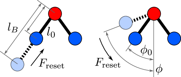
Figure 1: Intramolecular degrees of freedom in the water molecule modeled as harmonic displacements: Bond stretching (Eq. 2) and angle bending (Eq. 3) between an oxygen atom (red) and an associated hydrogen atom (blue).

Mathematically, $N$-body physics is described by a set of coupled ordinary differential equations (ODEs),

$$m_{i}\frac{\mathrm{d}^{2}\vec{r}_{i}}{\mathrm{d}t^{2}}=-\vec{\nabla}_{i}V(\vec{r}_{0},\dots\vec{r}_{N})=\vec{F}_{i}(\vec{r}_{0},\dots\vec{r}_{N})\,,$$ (1)

for $N$ distinct particles with positions $\vec{r}_{i}$, masses $m_{i}$ and conservative forces $\vec{F}_{i}$ generated by the potential energy $V$ with $\nabla_{i}^{d}=\partial/\partial r^{d}_{i}$ being the $d$th component of the gradient. The system (1) is an ODE of second order in time and first order in space.

2.1 Physical content: CHARMM force fields

The physical content encoded in the potential $V$ is a macroscopic theory where no quantum effects are involved. Water models are among the most popular parts of theoretical biophysics, as water is a very important solvent and a rather complex system. Different water models for digital computers have been suggested, implementing different properties that have been experimentally studied in real water. These water models vary in their computational complexity and accuracy and need to be chosen for the specific purpose of a study. Typically, the potential is a sum of bounded (intramolecular) and unbounded (intermolecular) contributions. Here, the typical constituents for the CHARMM (short for Chemistry at HARvard Macromolecular Mechanics) force fields will be reviewed [8, 9].

First, for intramolecular contributions, one typically considers bond stretching with a quadratic potential (c. f. Figure 1)

$$V_{b}=\sum_{bonds}k_{b}/2~{}(l_{b}-l_{0})^{2}$$ (2)

with force constant $k_{b}$ and bond length difference $l_{b}-l_{0}$ indicating deflection from equilibrium. Angle bending also models the bond angle deflection as a quadratic potential

$$V_{\phi}=\sum_{angles}k_{\phi}/2~{}(\phi-\phi_{0})^{2}\,.$$ (3)

Other contributions are obtained from dihedral angles, which are clockwise angles between two planes, where the planes are spanned between three respective atoms. The potential terms include quadratic contributions for proper and improper dihedrals. Since they only apply for molecules with $N\geq 4$ atoms, we won’t consider them here.

Next, for intermolecular contributions, one typically considers Van-der-Waals forces, which are modeled by Lennard-Jones potentials

$$V_{vdW}=\sum_{i,j|i<j}4\varepsilon_{i,j}\left[\left(\frac{\sigma_{i,j}}{r_{i,j}}\right)^{12}-\left(\frac{\sigma_{i,j}}{r_{i,j}}\right)^{6}\right]\,.$$ (4)

The polynomial potential (4) for uncharged atoms or molecules combines attracting and repelling forces. Indices $i$ and $j$ count over the atoms in the sum, $r_{i,j}$ is defined as the modulus of the position vectors $r_{i}$ and $r_{j}$ for atoms $i$ and $j$. $\varepsilon_{i,j}$ denotes the $y$-coordinate of the minimum in the potential and $\sigma_{i,j}$ describes the $x$-coordinate of the position where $V_{vdW}=0$.

Both inter- and intramolecular electrostatic interactions of the charged nuclei are modeled in a straightforward fashion with the Coulomb potential

$$V_{el}=\sum_{i,j|i<j}\frac{q_{i}q_{j}}{4\pi\varepsilon_{0}r_{i,j}},$$ (5)

which describes the interaction between atoms $i$ and $j$ with charges $q_{i}$ and $q_{j}$ and their position vector difference $r_{i,j}$ as in the Lennard-Jones potential. $\varepsilon_{0}$ denotes the dielectric constant.

Note that the older and currently most widely used models are rigid models which do not allow for polarization of the water molecule. All internal degrees of freedom are fixed and there are no dummy charges which would allow for polarization. They differ in their parameters for the force field and are purposely fitted to model-specific physical properties of water such as the diffusion coefficient, viscosity and others. Prominent examples here are the TIP3P and SPC/E water models [10].

Newer generations of water models introduce dummy charges to allow for a change in polarization and dipole moment within the water molecule. All internal degrees of freedom are still held static but the introduction of the dummy charges allows for the negative charges to be not entirely focused on the oxygen atom but to be located on the oxygen atom and a dummy charge below it (TIP4P) or dummy charges simulating the valence electron pairs of the oxygen atom (TIP5P). These approaches are computationally less costly than the introduction of flexible bounds but are still not used extensively as their computational costs are much higher than for models without polarization.

2.2 A single molecule demonstrator model

We want to simulate a single H₂O molecule with internal dynamics described by Coulomb forces, bond stretching and angle bending. Due to the limited size of the analog computer available, the problem is reduced to $d=2$ spatial dimensions instead of a full $d=3$ model. Furthermore, the angle bending is modelled using a small-angle approximation, i. e. replaced by a spring between the two hydrogen atoms, which is valid for small angular excitations.

For a single molecule in two dimensions, we have $N=3$ particles ($H_{1},H_{2},O$) and $D=2$ dimensions ($x,y$). Generally, the indices are given by $i\in(0,1,2)\equiv(O,H_{1},H_{2})$ and $d\in(0,1)\equiv(x,y)$. The equations of motions for the miniature force field are

$$\frac{\mathrm{d}\vec{v}_{i}}{\mathrm{d}t} =\sum_{j=0}^{N-1}\left(\left(1-\frac{l_{ij}}{r_{ij}}\right)k_{ij}+\frac{q_{i}q_{j}}{r_{ij}^{3}}\right)\frac{\vec{r}_{i}-\vec{r}_{j}}{m_{i}}\,,$$ (6a)

$$\frac{\mathrm{d}\vec{r}_{i}}{\mathrm{d}t} =\vec{v}_{i}\,.$$ (6b)

The spring rate matrix $$k_{ij}$$

models that either bond stretching ($k_{OH}$) happens between an oxygen and an hydrogen atom or angle bending ($k_{HH}$) is taking place between the two hydrogen atoms, c. f. figure 2. The rest positions $l_{ij}$ follow a similar definition with bond length $l_{OH}$ and the HH distance $l_{HH}$.

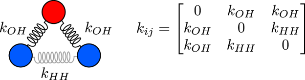
Figure 2: Simplified intermolecular forces modeling attracting ($k_{HH}$) and repelling ($k_{OH}$) forces on a purely harmonic approximation. This is implemented in the equations of motions (6).

2.3 Physical units

We have chosen a suitable natural unit system where all constants are within a reasonable size between zero and one. We measure the electric charges in multiples of the elementary chage $e=1$ and thus have $q_{O}=q_{0}=0.417$ and $q_{H}=q_{1,2}=-0.834$. The masses are measured in units of atomic mass units, $m_{O}=m_{0}=16$ and $m_{H}=m_{1}=m_{2}=1$. The vacuum permittivity is set to $4\pi\varepsilon_{0}=1$. Lengths are measured in Å, and therefore the distance at rest (bound length) between OH is given by $l_{B}=0.9572:=l_{OH}$. The opening angle at the Oxygen atom is $104^{\circ}=0.58\pi$, which determines the distance at rest between HH as $l_{HH}=2\,l_{OH}\sin(0.58\pi/2)$.

2.4 Properties and limitations

The characteristic frequencies or normal modes of molecules [11] are often taken into account when reasoning about the validity of a force field or its numerical simulation. In $d=3$ spatial dimensions, a single water molecule has $9$ well-known modes, such as the symmetric, anti-symmetric and bending mode. Due to the non-orthogonal geometry of our spring model (6), one cannot expect these modes to appear when $k_{HH}\neq 0$. This is mainly because the small angle approximation is violated by the HH spring. On the other hand, with $k_{HH}=0$, nothing prevents the $OH$ binding from rotating around the oxygen atom. The angle bending approximation is a computationally cheap choice for avoding these non-physical oscillations.

For solvent models, a number of statistically or thermodynamically derived quantities are typically considered in benchmarks [12], such as the temperature, potential energy and equilibirium stability of a large molecular ensemble. The self-diffusion coefficient and the radial distribution functions for water can be tested and are meaningful properties of a physical model (force field) and the applied computational methods which have been used. With a single molecule, there is no meaningful equivalent.

3 Analog computer implementation

The classical equations of motions (1) are coupled ordinary differential equations. In contrast to classical fluid dynamics, where the time evolution of some field $F(\vec{x},t)$ is determined by a partial differential equation, ordinary differential equations of distinct particle trajectories $\vec{r}(t)$ can be directly mapped to electrical circuits. The traditional direct approach represents all vectorial components $i$ of the involved particles $j$ by one connection between computing elements per degree of freedom $\boldsymbol{r}^{i}_{j}(t)$. Following this approach, all intermediate computing results are also represented this way, such as velocities $\boldsymbol{v}^{i}_{j}(t)$ and any algebraic (sub-)expression encountered in the particular analytically defined equation of motion. Note that time is kept continous while the discretization follows the concepts of discrete and distinguishable particles in classical physics.

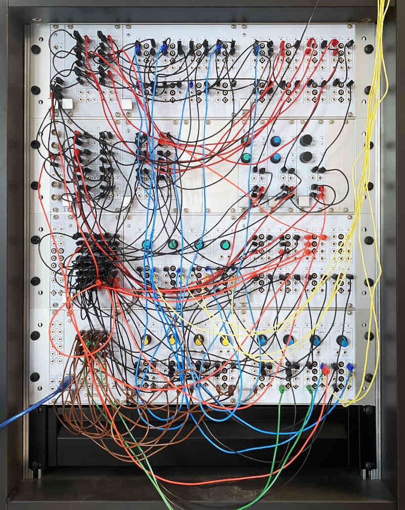
Figure 3: Photography of the front panel of a large analog computer of type Analog Paradigm Model-1, implementing equations (7) in a scaled manner (c. f. section 3).

3.1 Naming all constitutional parts of the equation

In order to implement the equation of motions on the analog computer, one has to decompose the equation into the primitive analog computing elements. In general, upper indices will indicate the vector index $\cdot^{d}$, while lower indices $\cdot_{i}$ indicate the particle index. Bold face is used to separate the name of a variable (connection) whereas indices are given in regular form, which is particular relevant for the multiplicative inverses, such as the distance matrix $\boldsymbol{r}^{\boldsymbol{-1}}_{ij}$. It is computed as following:

$$\boldsymbol{r}_{ij}^{d}=r_{i}^{d}-r_{j}^{d}\,,\quad\boldsymbol{s}^{d}_{ij}=\left(\boldsymbol{r}_{ij}^{d}\right)^{2}\,~{}~{}\text{and}~{}~{}$$ (7a)

$$\boldsymbol{t}_{ij}=\textstyle\sum_{k}^{D}\boldsymbol{s}_{ij}^{k}\,,~{}~{}\text{so that}~{}~{}\boldsymbol{r}^{\boldsymbol{-1}}_{ij}=1/\sqrt{\boldsymbol{t}_{ij}}\,.$$ (7b)

Note that the coordinate difference components $$\boldsymbol{r}^{d}_{ij}=-\boldsymbol{r}^{d}_{ji} \boldsymbol{r}_{ij} \boldsymbol{r}^{\boldsymbol{-1}}_{ij} \boldsymbol{r}_{ij}=\boldsymbol{r}_{ji} \boldsymbol{r}_{ii}=0 \boldsymbol{r}_{ij}\in\mathbb{R}^{M\times D} M=(N^{2}-N)/2=3$$ are antisymmetric. The distance matrix and its multiplicative inverse are symmetric () and traceless (). Thus one only has to compute many elements, with . The actual force components

$$\boldsymbol{F}_{ij}^{d}=\left(\left[l_{ij}{\boldsymbol{r}}_{ij}^{\boldsymbol{-1}}-1\right]k_{ij}+\frac{q_{i}q_{j}}{\varepsilon_{0}}({\boldsymbol{r}}_{ij}^{\boldsymbol{-1}})^{3}\right)\boldsymbol{r}_{ij}^{d}$$ (7c)

are antisymmetric and traceless ($$\boldsymbol{F}^{d}_{ij}=-\boldsymbol{F}^{d}_{ji} \boldsymbol{F}^{d}_{ii}=0 i,j,d \Delta_{ij}$$ and for all ). Also note that the bond stretching is only applied between H and O atoms of a single molecule, which is encoded in . The velocity and position components can be determined by analog time integration

$$\boldsymbol{v}_{i}^{d}=-\int_{t}\mathrm{d}t\sum_{j}^{N}\left(-\frac{\boldsymbol{F}_{ij}^{d}}{m_{i}}\right),\quad\boldsymbol{r}_{i}^{d}=-\int_{t}\mathrm{d}t~{}(-\boldsymbol{v}_{i}^{d}),$$ (7d)

where the notation is oriented on the negating nature of the analog computing elements.

3.2 Machine realization

The set of equations (7) is directly mapped to the general purpose analog computing elements of the Analog Paradigm Model-1 computer we used in this simulation [13]. The overall circuit is given in Appendix 5 and is a 1:1 translation of the mathematical expressions (7). We would like to emphasize that on this level of abstraction, the abstract syntax tree of the mathematical expressions is identical to the equivalent circuit. The physical realization of this particular analog computer program is shown in figure 3. The machine is equipped with a Hybrid Controller (it can be identified by its USB cable in the lower left of figure 3). The system can be fully configured from an attached digital computer to set the model’s constants and parameterers; there are more then 30 digital potentiometers involved, each with a resolution of 10 bit.

4 Circuit scaling

The question of value ranges and domain sizes is crucial in any (analog or digital) computer simulation of a physical problem. This topic is typically not given much attention in presentations of novel numerical codes. When implementing analog circuits, ensuring the correct scaling of the solution is an inherent part of the problem mapping. Various aspects of this scaling process are discussed here.

4.1 Analog number representation

For number representation on computers, it is essential that quantities do not exceed the valid range of values. For instance, a signed 32 bit integer can store values between 0 and $2^{31}\approx 10^{10}$. In contrast, the IEEE 754 floating point number representation allows to represent numbers up to $2^{127}\approx 10^{38}$, which comes with a loss of precision. When doing numerical computations, any number outside the valid data range results in an overflow and an invalid result. However, on a digital computer, there is always the possibility to use longer bit sequences to represent numbers. For instance, one could use a double-precision floating point number representation with a width of 64 bit, allowing numbers up to $2^{1023}\approx 10^{308}$. The same applies for numbers which are bounded by nature, for instance percentages or saturations. If a number $p\in[0,1]$ is to be represented on a digital computer, then the 32 bit signed integer will naturally represent $p$ with a uniform accuracy of $\Delta p\approx 10^{-38}$. In contrast, 32 bit single-precision floating point has a precision $\Delta p\approx 10^{-20}$ for values down to $10^{-12}$ and up to $\Delta p\approx 10^{-8}$ for values close to $1$.

The success and widespread use of floating point numbers makes number representation a topic, which numerical scientists only have to deal in special cases, for instance when it comes to instabilities, catastrophic cancellation or the like. In day-to-day work, the occurence of an out-of-bound value (represented as NaN, not a number, in the IEE754 standard) is typically a sign of a programming error, such as computing $1/0$ resulting from an uninitialized or in some way “illegal” denominator.

In electronic analog computers, numbers are typically represented as voltages or currents. Given the fixed physical structure of such a computer, these quantities are bounded in principle. On an information theoretical level, such computing elements are called “bounded in, bounded out” (BIBO) [14]. The illegality of non-bounded values is similar as to the behaviour of number representations in digital computing. For the time being, let’s assume the valid range for a value in an analog computer to be $[-1,+1]$.

Analog computers have an inherent limited precision of about three to four decimal places [15]. In the above convention, this yields a precision $\Delta p\approx 10^{-4}$ which is roughly the resolution of a half-precision floating point number or 10 to 16 bits of information.

In order to answer the question of whether simulating water molecules on an analog computer can compare to current digital simulations, given the limitations in resolution of the analog computer, we assume the Coulomb potential terms to be the limiting factor. Keep in mind that in the present study we can neglect the Lennard-Jones potential as we are only modelling a single molecule.

4.2 Coordinate units

To improve readability, we assume a physical square simulation domain of size $\Omega:=[-L,+L]^{D}$ with some dimensionful length scale $L$ in $D$ spatial dimensions with any physical coordinate $\boldsymbol{r}^{d}_{i}\in\Omega$. Scaled and dimensionless units can be easily recovered as $\hat{r}:=r/L\in\hat{\Omega}$ contained in a unit domain $\hat{\Omega}=[-1,+1]^{D}$. In practice that means that initial values have to be scaled according to $\hat{r}_{i}^{d}(0)=r_{i}^{d}(0)/L$ and $\hat{v}^{i}_{d}(0)=v_{i}^{d}(0)/L$. Also the distances at rest $l_{OH}$, $l_{HH}$ and the de facto Coulomb coupling constant $\varepsilon_{0}$ have to be chosen in physical units before transformation.

Assuming that each mapping in (7a) has a bounded input on the right hand side of the definition, the following scaling has to be applied to ensure bounded output:

$$\hat{\boldsymbol{r}}_{ij}^{d}:=\frac{\hat{r}_{i}^{d}-\hat{r}_{j}^{d}}{\alpha}\,,\quad\hat{\boldsymbol{s}}^{d}_{ij}:=\left(\hat{\boldsymbol{r}}_{ij}^{d}\right)^{2}\,,\quad$$ (8)

$$\hat{\boldsymbol{t}}_{ij}:=\frac{\textstyle\sum_{k}^{D}\hat{\boldsymbol{s}}_{ij}^{k}}{\delta^{2}}\,,\quad\hat{\boldsymbol{r}}^{\boldsymbol{-1}}_{ij}:=1/\left({\beta\sqrt{\hat{\boldsymbol{t}}_{ij}}}\right)\,.$$ (9)

Three factors were introduced: Two geometric ones ($\alpha$ and $\delta$) resulting from the dimensionless coordinate representation and an internal one ($\beta$) to deal with the multiplicative inverse (reciprocal). These scaling factors sum up to

$$\hat{\boldsymbol{r}}^{\boldsymbol{-1}}_{ij}:=\gamma\,\boldsymbol{r}^{\boldsymbol{-1}}_{ij}$$ (10)

with overall scaling factor $\gamma:=\alpha\delta/\beta$. Note that applying this scaling means that $\hat{\boldsymbol{r}}^{-1}_{ij}\neq 1/|\hat{\boldsymbol{r}}_{i}-\hat{\boldsymbol{r}}_{j}|$, i. e. a clear relationship between the “hatted” quantities $\hat{\boldsymbol{r}}_{\dots}$ no longer exists. The neccessity and implications of the individual factors are discussed below.

4.2.1 Geometric scaling

The factor $\alpha$ has two contributions determined by the maximum possible distance of two particles in both $D$ dimensions ($d_{\text{max}}=\sqrt{D}$) and one dimension, where $d_{\text{max}}=2$ and $1\leq\alpha\leq 2$ is a sensible choice. The factor $\delta$ results from the sum of $D$ scaled quantities. A useful choice might be $\delta=\sqrt{D}$. Both factors $\alpha$ and $\delta$ are optional as they might be applied but their underlying scaling problems can also be neglected in practice if no overflow problems occur. In order to simplify the reasoning, the optional factors are neglected for the rest of the text, so $\alpha=\delta=1$ and thus $\gamma=1/\beta$.

4.2.2 Inverse-square law scaling

The factor $\beta$ is due to the necessity of computing multiplicative inverses on BIBO unit domains. It is crucial and must not be omitted. Displaying an inverse-square law such as the Coulomb potential $V_{ij}(d)\sim 1/r_{ij}$ or the electrostatic force $F_{ij}(d)\sim 1/r_{ij}^{2}$ with $r_{ij}=|\vec{r}_{i}-\vec{r}_{j}|$ being the distance between two particles $i$ and $j$ on an analog computers is challenging, since it is immediately $1/r_{ij}>1$ for $r_{ij}<1$. The approach in (8) is to apply a scaling factor $1/\beta\ll 1$ on $\boldsymbol{r^{-1}}$. This allows the distance component $\boldsymbol{t}_{ij}$ to become as small as $\beta^{-2}$ (because for smaller $\boldsymbol{t}_{ij}<\beta^{-2}$, again $\boldsymbol{r^{-1}}>1$). Naturally, this introduces an ultraviolet cutoff at $\beta^{-1}$. If two particles come closer than $\beta^{-1}$, their distances can no longer be represented on the computer. Cutoffs are a well-understood phenomenon in theoretical physics and also occur in numerical simulations.

4.3 In-circuit scaling

The scaling coefficients $\alpha,\beta,\delta$ are not relevant outside the computation. Instead, they only affect the potentiometer values. By convention, the scaling factors (lowercase greek letters as $\alpha$) are typically outside the BIBO range $[-1,+1]$, while the potentiometer values (uppercase Fraktur letters as $\mathfrak{A}$) are within.

4.3.1 Force scaling

The system force (7c) is scaled as

$$\hat{\boldsymbol{F}}^{d}_{ij}:=\zeta\frac{{\boldsymbol{F}}^{d}_{ij}}{\beta^{3}}$$ (11)

The factor $\beta^{3}$ results from the linear dependency on $\boldsymbol{r}^{-3}$, which implies carrying on the scaling. The factor $\zeta>1$ is an non-nphysical scaling factor introduced in order to allow force amplification in the subsequent steps.

By replacing unscaled quantities in (7c) by their scaled counterparts of the previous section, the potentiometer values are determined as:

$$\hat{\boldsymbol{F}}^{d}_{ij}:=\Bigg{[}\left(\frac{l_{ij}}{\beta^{2}}~{}\frac{\hat{\boldsymbol{r}}^{\boldsymbol{-1}}_{ij}}{\beta}-\frac{1}{\beta^{3}}\right)k_{ij}+\frac{q_{i}q_{j}}{\varepsilon_{0}}\frac{\hat{\boldsymbol{r}}^{\boldsymbol{-3}}_{ij}}{\beta^{3}}\Bigg{]}\zeta~{}{\hat{\boldsymbol{r}}^{d}_{ij}}$$ (12)

With the intention to define parameters $\mathfrak{P}$, which directly map on a single potentiometer with range $0\leq\mathfrak{P}\leq 1$ on the Model-1, we introduce the quantities

$$\mathfrak{R}_{ij}=\zeta\frac{l_{ij}k_{ij}}{\beta^{2}}\,,\quad\mathfrak{U}_{ij}=\zeta\frac{k_{ij}}{\beta^{3}}\,,\quad\mathfrak{C}_{ij}=\zeta\frac{|q_{i}q_{j}|}{\varepsilon_{0}}\,.$$ (13)

The scaled force is then

$$\hat{\boldsymbol{F}}^{d}_{ij}=\left({\mathfrak{R}_{ij}}~{}\frac{\hat{\boldsymbol{r}}^{\boldsymbol{-1}}_{ij}}{\beta}-{\mathfrak{U}_{ij}}\pm\mathfrak{C}_{ij}\,\frac{\hat{\boldsymbol{r}}^{\boldsymbol{-3}}_{ij}}{\beta^{3}}\right){\hat{\boldsymbol{r}}^{d}_{ij}}\,.$$ (14)

One has to take care of the sign in front of $\mathfrak{C}_{ij}$, which is $-1$ for OH interactions and $+1$ for HH interactions. The required negation is indicated by $\pm$ in (14). When following the scaling argument $\delta$ of the previous section, (14) would also require a factor $1/3$ to compensate the sum of three scaled quantities. However, due to the different orders of magnitude of the coupling constants, this scaling choice was not considered here.

4.3.2 Time integration

The standard analog time integration [16] reads

$$e_{0}=-\left(\int_{0}^{t}k_{0}\mathrm{d}t^{\prime}\sum_{r=1}^{n}a_{r}e_{r}(t^{\prime})\right)-e(0)$$ (15)

with initial condition $e(0)$, inputs $e_{r}$, output $e_{0}$, input weights $a_{r}$, time scale factor $k_{0}$ and machine time $t^{\prime}=t/k_{0}$. On the Model-1 analog computer, possible input weights are $a_{i}\in\{1,10\}$ and $k_{0}\in\{10,100,1000\}$. These have to be chosen at programming time. For the velocity and coordinate integration, we can compute physical quantities $\hat{\boldsymbol{v}}_{i}^{d}\equiv\boldsymbol{v}_{i}^{d}$ and $\hat{\boldsymbol{r}}_{i}^{d}\equiv\boldsymbol{r}_{i}^{d}$ by carefully reversing all scaling operations. We do so by casting (7d) as

$$\boldsymbol{-}\hat{\boldsymbol{v}}_{i}^{d} =-\int_{0}^{t}k_{0}\,\mathrm{d}t\sum_{j}^{N}\left(a_{i}\frac{1}{m_{i}}\,{\boldsymbol{F}_{ij}^{d}}\right)$$ (16)

$$=-\int_{0}^{t}k_{0}\,\mathrm{d}t\sum_{j}^{N}\left(a_{i}\frac{1}{m_{i}}\frac{\beta^{3}}{\zeta}\,{\hat{\boldsymbol{F}}_{ij}^{d}}\right)$$ (17)

$$=-\int_{0}^{t}k_{0}\,\mathrm{d}t\sum_{j}^{N}\left(\mathfrak{F}_{i}\,{\hat{\boldsymbol{F}}_{ij}^{d}}\right)\,.$$ (18)

We introduced the potentiometer value

$$\mathfrak{F}_{i}=\frac{1}{m_{i}}\frac{\beta^{3}}{\zeta}\frac{1}{a_{i}}\,.$$ (19)

Thanks to moving the integrator weight $a_{i}$ into $\mathfrak{F}_{i}$, it can be ensured that $\mathfrak{F}_{i}\leq 1$ for many weight choices. If this is not sufficient, one can still make use of the timescale factors $k_{0}$ for an additional degree of freedom in scaling. In our setup all integrators have the same $k_{0}$ which is thereby solely responsible for the speed of integration (or simulation vs. realclock time ratio). On future chip-level generations, $k_{0}\approx 10^{7}$ is expected [1]. The velocity integration is then trivially given by

$$\hat{\boldsymbol{r}}_{i}^{d}=-\int_{0}^{t}k_{0}\mathrm{d}t~{}(\boldsymbol{-}\hat{\boldsymbol{v}}_{i}^{d})\,.$$ (20)

4.3.3 Numerical potentiometer values

With $\beta=5$ and the physical units given in section 2.3, we obtain $\mathfrak{R}_{HH}=0.036\zeta$, $\mathfrak{R}_{OH}=0.04\zeta$, $\mathfrak{C}_{ij}=(\pm)0.0139\zeta$ and $\mathfrak{U}_{ij}=0.008\zeta$. These small numbers suggest to upscale the forces with $\zeta=30$. This results in $\mathfrak{F}_{0}=\beta^{3}/\zeta/m_{O}=125/16/30=0.2594$ with $a_{0}=1$ and $\mathfrak{F}_{1}=\mathfrak{F}_{2}=\beta^{3}/m_{H}/\zeta/10=125/30/10=0.4166$ with $a_{1}=a_{2}=10$.

4.4 Conclusions on the dynamical range

In the last section, we came up with a value scaling, which introduces a cutoff at a length scale $\beta^{-1}$. With typical choices $\beta\sim 10$, this introduces basically a minimal length the order of $L_{\text{min}}=1/\beta\sim 0.1$. Equally, the maximum length in the simulation domain is determined by the BIBO domain size, i. e. $L_{\text{max}}=1$. Note that the minimal length is not a rounding/resolution error (as a $\Delta x$ would be in a numerical approach). The computational exactness (rounding error) of an analog computer is of the order of $10^{-5}\ll L_{\text{min}}$.

$L_{\text{min}}$ provides a minimal distance between two atoms, so it is the limiting factor in terms of precision. Chemical bonds like the O-H distance are of the order of magnitude of 1 Å while the valid range of the entire water box runs from $-1$ analog units to $+1$ analog units. Identifying $L_{\text{min}}$ analog units with 1 Å in the water box a maximum side length for a water box of 20 Å or 2 nm is possible. Most water boxes are in the nanometer range, so this value representation might be applicable to tackle real world simulations. Nevertheless we acknowledge that it might be too small to contain large macromolecules and different value representations or digital assisted approaches may be neccessary in future work.

5 Complete Circuit

The overall circuit of the setup shown in Figure 3 is described below. All indices and sums are written out and are fully scaled. Note that we moved some constants between the definitions (for instance between $F$ and $C$).

A triangular shape denotes a summer (with implicit change of sign), while a polygon with a large $\Pi$ represents a multiplier, divider or square root component. Circles represent coefficient potentiometers and rectangles with attached triangles are integrators.

5.1 Computing distance components $r^{i}_{jk}$, $s^{i}_{jk}$ and $t_{jk}$

$$\begin{aligned} r^{0}_{01}&=-(-r_{0}^{0})+(-r_{1}^{0})\\ r^{0}_{02}&=-(-r_{0}^{0})+(-r_{2}^{0})\\ r^{0}_{12}&=-(-r_{1}^{0})+(-r_{2}^{0})\\ r^{1}_{01}&=-(-r_{0}^{1})+(-r_{1}^{1})\\ r^{1}_{02}&=-(-r_{0}^{1})+(-r_{2}^{1})\\ r^{1}_{12}&=-(-r_{1}^{1})+(-r_{2}^{1})\end{aligned}\qquad\begin{aligned} s^{0}_{01}&=(r^{0}_{01})^{2}\\ s^{0}_{02}&=(r^{0}_{02})^{2}\\ s^{0}_{12}&=(r^{0}_{12})^{2}\\ s^{1}_{01}&=(r^{1}_{01})^{2}\\ s^{1}_{02}&=(r^{1}_{02})^{2}\\ s^{1}_{12}&=(r^{1}_{12})^{2}\end{aligned}$$ (21)

$$t_{01}=s^{0}_{01}+s^{1}_{01}\quad~{}~{}~{}t_{02}=s^{0}_{02}+s^{1}_{02}\quad~{}~{}~{}t_{12}=s^{0}_{12}+s^{1}_{12}$$

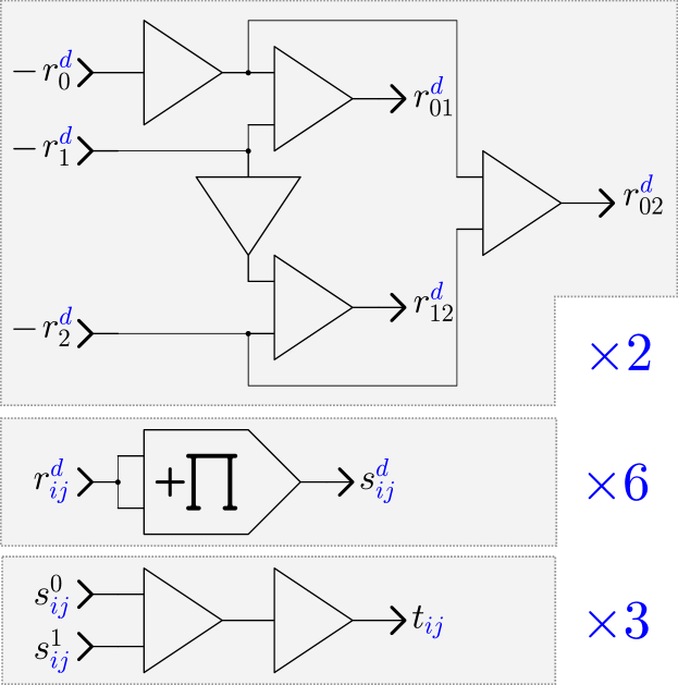
Figure 4: Computing $r^{i}_{jk}$, $s^{i}_{jk}$, and $t_{jk}$, as in equation (21).

5.2 Computing inverse distances $\boldsymbol{r^{-1}}$ and their cubes

The scaling with $\beta$ is applied in the circuit (figure 5) before applying the division. A single potentiometer for $\beta^{-1}$ is sufficient as an input for all three divisions.

$$\begin{aligned} \frac{\boldsymbol{r}^{\boldsymbol{-1}}_{01}}{\beta}&=\beta^{-1}/\sqrt{t_{01}}\\ \frac{\boldsymbol{r}^{\boldsymbol{-1}}_{02}}{\beta}&=\beta^{-1}/\sqrt{t_{02}}\\ \frac{\boldsymbol{r}^{\boldsymbol{-1}}_{12}}{\beta}&=\beta^{-1}/\sqrt{t_{12}}\end{aligned}\qquad\qquad\begin{aligned} \frac{\boldsymbol{r}^{\boldsymbol{-3}}_{01}}{\beta^{3}}&=(\boldsymbol{r}^{\boldsymbol{-1}}_{01})^{3}/\beta^{3}\\ \frac{\boldsymbol{r}^{\boldsymbol{-3}}_{02}}{\beta^{3}}&=(\boldsymbol{r}^{\boldsymbol{-1}}_{02})^{3}/\beta^{3}\\ \frac{\boldsymbol{r}^{\boldsymbol{-3}}_{12}}{\beta^{3}}&=(\boldsymbol{r}^{\boldsymbol{-1}}_{12})^{3}/\beta^{3}\end{aligned}$$ (22)

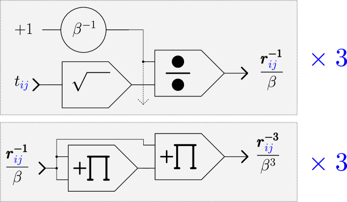
Figure 5: Computing $\frac{r^{-1}_{jk}}{\beta}$ and $\frac{r^{-3}_{jk}}{\beta^{3}}$, according to equation (22).

5.3 Computing the forces

$$\frac{\boldsymbol{F}^{0}_{01}}{\beta^{3}} =\Big{(}{\mathfrak{R}_{01}}~{}\frac{\boldsymbol{r}^{\boldsymbol{-1}}_{01}}{\beta}-{\mathfrak{U}_{01}}~{} -~{}\mathfrak{C}_{01}\frac{\boldsymbol{r}^{\boldsymbol{-3}}_{01}}{\beta^{3}}\Big{)}r^{0}_{01}$$ (23)

$$\frac{\boldsymbol{F}^{0}_{02}}{\beta^{3}} =\Big{(}{\mathfrak{R}_{02}}~{}\frac{\boldsymbol{r}^{\boldsymbol{-1}}_{02}}{\beta}-{\mathfrak{U}_{02}} -~{}\mathfrak{C}_{02}\frac{\boldsymbol{r}^{\boldsymbol{-3}}_{02}}{\beta^{3}}\Big{)}r^{0}_{02}$$

$$\frac{\boldsymbol{F}^{0}_{12}}{\beta^{3}} =\Big{(}\mathfrak{R}_{12}~{}\frac{\boldsymbol{r}^{\boldsymbol{-1}}_{01}}{\beta}-\mathfrak{U}_{12} +~{}\mathfrak{C}_{12}\frac{\boldsymbol{r}^{\boldsymbol{-3}}_{12}}{\beta^{3}}\Big{)}r^{0}_{12}$$

$$\frac{\boldsymbol{F}^{1}_{01}}{\beta^{3}} =\Big{(}{\mathfrak{R}_{01}}~{}\frac{\boldsymbol{r}^{\boldsymbol{-1}}_{01}}{\beta}-{\mathfrak{U}_{01}}~{} -~{}\mathfrak{C}_{01}\frac{\boldsymbol{r}^{\boldsymbol{-3}}_{01}}{\beta^{3}}\Big{)}r^{1}_{01}$$

$$\frac{\boldsymbol{F}^{1}_{02}}{\beta^{3}} =\Big{(}{\mathfrak{R}_{02}}~{}\frac{\boldsymbol{r}^{\boldsymbol{-1}}_{02}}{\beta}-{\mathfrak{U}_{02}} -~{}\mathfrak{C}_{02}\frac{\boldsymbol{r}^{\boldsymbol{-3}}_{02}}{\beta^{3}}\Big{)}r^{1}_{02}$$

$$\frac{\boldsymbol{F}^{1}_{12}}{\beta^{3}} =\Big{(}{\mathfrak{R}_{12}}~{}\frac{\boldsymbol{r}^{\boldsymbol{-1}}_{02}}{\beta}-{\mathfrak{U}_{12}} +~{}\mathfrak{C}_{12}\frac{\boldsymbol{r}^{\boldsymbol{-3}}_{12}}{\beta^{3}}\Big{)}r^{1}_{12}$$

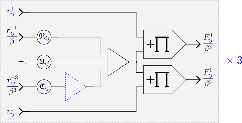
Figure 6: Computing $\frac{F^{i}_{jk}}{\beta^{3}}$ as in equation (23). Note that the negator indicated in dotted lines is only placed when computing $F^{d}_{01}$ and $F^{d}_{02}$ but not $F^{d}_{12}$.

5.4 Computing velocities and positions

Note how the signs in front of $\mathfrak{F}_{i}$ result from symmetries carried out (c. f. section 3.1).

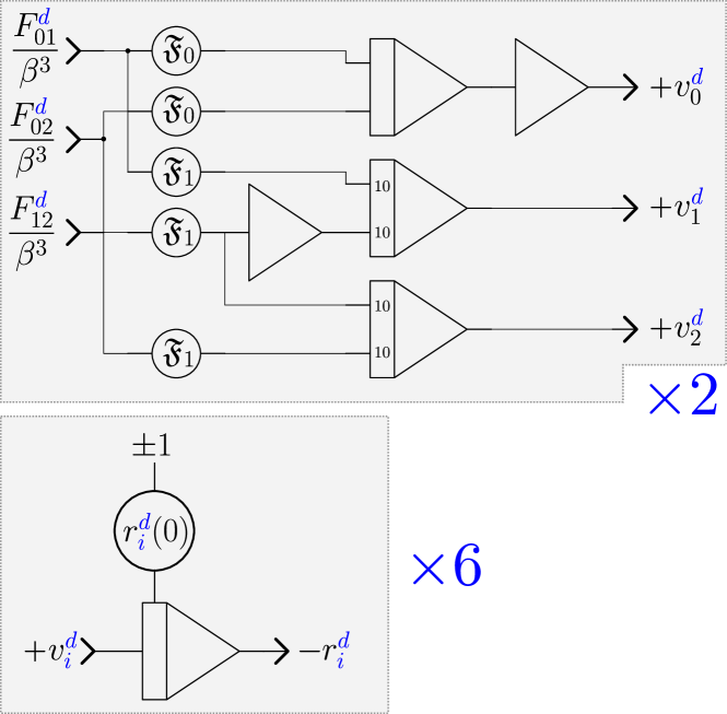
Figure 7: Computing $v^{i}_{j}$ and $r^{i}_{j}$, as in equation (26).

$$-\boldsymbol{v}_{0}^{0} =-\int^{t}_{0}k_{0}\,\mathrm{d}t\left(+\mathfrak{F}_{0}\cdot\beta^{3}~{}\frac{F_{01}^{0}}{\beta^{3}}+\mathfrak{F}_{0}\cdot\beta^{3}~{}\frac{F_{02}^{0}}{\beta^{3}}\right)$$ (24)

$$-\boldsymbol{v}_{1}^{0} =-\int^{t}_{0}k_{0}\,\mathrm{d}t\left(-\mathfrak{F}_{1}\cdot\beta^{3}~{}\frac{F_{01}^{0}}{\beta^{3}}+\mathfrak{F}_{1}\cdot\beta^{3}~{}\frac{F_{12}^{0}}{\beta^{3}}\right)$$

$$-\boldsymbol{v}_{2}^{0} =-\int^{t}_{0}k_{0}\,\mathrm{d}t\left(-\mathfrak{F}_{1}\cdot\beta^{3}~{}\frac{F_{02}^{0}}{\beta^{3}}-\mathfrak{F}_{1}\cdot\beta^{3}~{}\frac{F_{12}^{0}}{\beta^{3}}\right)$$

$$\Leftrightarrow+\boldsymbol{v}_{2}^{0} =+\int^{t}_{0}k_{0}\,\mathrm{d}t\left(+\mathfrak{F}_{1}\cdot\beta^{3}~{}\frac{F_{02}^{0}}{\beta^{3}}+\mathfrak{F}_{1}\cdot\beta^{3}~{}\frac{F_{12}^{0}}{\beta^{3}}\right)$$

$$-\boldsymbol{v}_{0}^{1} =-\int^{t}_{0}k_{0}\,\mathrm{d}t\left(+\mathfrak{F}_{0}\cdot\beta^{3}~{}\frac{F_{01}^{1}}{\beta^{3}}+\mathfrak{F}_{0}\cdot\beta^{3}~{}\frac{F_{02}^{1}}{\beta^{3}}\right)$$ (25)

$$-\boldsymbol{v}_{1}^{1} =-\int^{t}_{0}k_{0}\,\mathrm{d}t\left(-\mathfrak{F}_{1}\cdot\beta^{3}~{}\frac{F_{01}^{1}}{\beta^{3}}+\mathfrak{F}_{1}\cdot\beta^{3}~{}\frac{F_{12}^{1}}{\beta^{3}}\right)$$

$$-\boldsymbol{v}_{2}^{1} =-\int^{t}_{0}k_{0}\,\mathrm{d}t\left(-\mathfrak{F}_{1}\cdot\beta^{3}~{}\frac{F_{02}^{1}}{\beta^{3}}-\mathfrak{F}_{1}\cdot\beta^{3}~{}\frac{F_{12}^{1}}{\beta^{3}}\right)$$

$$\Leftrightarrow+\boldsymbol{v}_{2}^{1} =+\int^{t}_{0}k_{0}\,\mathrm{d}t\left(+\mathfrak{F}_{1}\cdot\beta^{3}~{}\frac{F_{02}^{1}}{\beta^{3}}+\mathfrak{F}_{1}\cdot\beta^{3}~{}\frac{F_{12}^{1}}{\beta^{3}}\right)$$

In our circuit, the initial data for the velocities are always zero, while initial data for the positions are fed in as initial conditions for the integrators (see figure 7).

$$\boldsymbol{r}_{0}^{0} =-\int^{t}_{0}(-v_{0}^{0})~{}k_{0}\,\mathrm{d}t-r^{0}_{0}(0)\,,$$ (26)

$$\boldsymbol{r}_{1}^{0} =-\int^{t}_{0}(-v_{1}^{0})~{}k_{0}\,\mathrm{d}t-r^{1}_{0}(0)\,,$$

$$\boldsymbol{r}_{2}^{0} =-\int^{t}_{0}(-v_{2}^{0})~{}k_{0}\,\mathrm{d}t-r^{2}_{0}(0)\,,$$

$$\boldsymbol{r}_{0}^{1} =-\int^{t}_{0}(-v_{0}^{1})~{}k_{0}-r^{0}_{1}(0)\,\mathrm{d}t\,,$$

$$\boldsymbol{r}_{1}^{1} =-\int^{t}_{0}(-v_{1}^{1})~{}k_{0}-r^{1}_{1}(0)\,\mathrm{d}t\,,$$

$$\boldsymbol{r}_{2}^{1} =-\int^{t}_{0}(-v_{1}^{1})~{}k_{0}-r^{2}_{1}(0)\,\mathrm{d}t\,.$$

6 Benchmarking the analog implementation

The model produces reasonable results for small perturbations, as shown in Figure 8 for a simulation time of $t_{\text{final}}=60$ms.

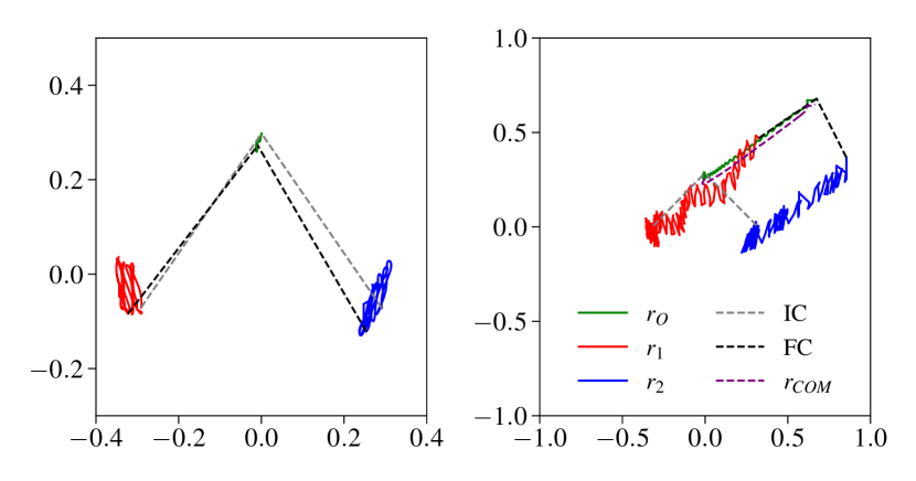
Figure 8: Analog water molecule simulation results. The left panel shows a closeup of a small excitation around the resting positions. The red and blue trajectories represent the two hydrogen atoms. The oxygen atom (green trajectory) is almost at rest. The OH binding is indicated by the dashed lines. The grey dashed lines show the initial condition (IC), while the dark dashed lines indicate the final condition (FC). The right panel shows a long time run which clearly shows the center of mass ($r_{COM}$, purple line) drifting along with the oxygen $r_{O}$.

.

6.1 Energy and time demand

The bending patterns have roughly a wall clock time frequency of $f\sim 100$ Hz, while the water bending normal modes have a frequency of $\nu\sim 32$ Ghz in nature. This gives an effective ratio of about $k\sim 10^{-9}$ for the analog implementation, or a simulation time per real clock time ratio of $100/32\sim 3\,$ns/s or 260 $\mu$s/day. This number has to be compared with typical simulations on digital computers, which achieve a few hundred ns per day (see for instance a review [17] and references therein, such as [18]).

It is a crucial property of analog computing that this speed factor is invariant of the size of the equation (and circuitry, respectively)! That it, it is virtually independent of both the number of particles simulated as well as the physics included (c. f. Section 2.1). In contrast, the power (and thus energy) requirements scale linearly with the size of the circuit [1]. The Analog Paradigm Model-1 power requirement for the present circuit is measured as $P_{A}=21$W. The overall energy requirement for a single bending wave is therefore $E_{A}=P_{A}T\sim 210$ mJ.

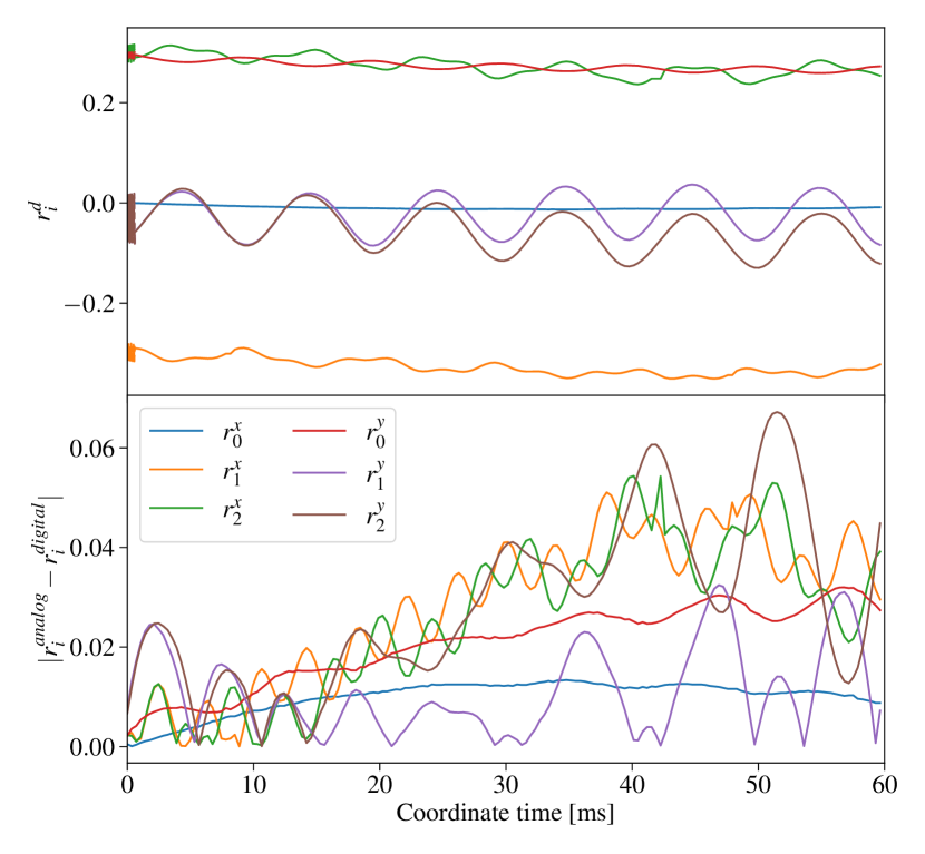
Figure 9: Upper panel: Analog (solid) vs. digital (dashed) time evolution. Lower panel: Absolute error (L1 norm) of digital vs. analog resuls for all particle coordinates $r^{d}_{i}$.

6.2 Upscaling: Towards real-life molecular dynamics

The overall number of computing elements required for this simulation can be obtained from the system equation (7) or the circuit schematics (Appendix 5). It scales with spatial dimensions $D$, number of atoms $N$ and reduced number of degrees of freedom $M=(N^{2}-N)/2$ as

$$(2D+1)M+2=5\cdot 3+2=17 \quad\times\text{SUM}~{}(\Sigma)$$

$$(2D+2)M=6\cdot 3=18 \quad\times\text{MUL}~{}(\Pi)$$

$$M=3 \quad\times\text{SQRT}~{}(\sqrt{\cdot})$$

$$2ND=2\cdot 3\cdot 2=12 \quad\times\text{INT}~{}(\smallint)\,.$$

Ignoring the different types of computing elements, one comes up with $\mathcal{O}(8N^{2})$ computing elements in $D=3$ dimensions. For instance, a typical water box in $D=3$ with a size of $($30\text{\,}\mathrm{\SIUnitSymbolAngstrom}$)^{3}$ and $N\sim 10^{4}$ atoms requires $7\times 10^{6}$ computing elements.

One can estimate the performance of such a simulation carried out on a future analog computer on a chip. To do so, the reasoning of [1] is employed. Moving from an Analog Paradigm Model-1 analog computer to a proposed analog computer on chip will decrease energy consumption by at least a factor of 40 with an increase in speed by a factor of at least 150. This results in a power demand for a fully integrated analog computer simulating $N\sim 10^{4}$ atoms of $P=10^{4}/3\times 20\text{W}/40\approx 1600$W with a simulation per real clock time ratio of more than $10^{7}$ ns/day!

While this number of computing elements is definetly in the ballpark of future analog computing chips, the number of interconnections is certainly the limiting factor. The quadratic dependency on $N$ is in fact dominated by the all-to-all force coupling $F_{ij}$ in Newtonian mechanics. Typically, a long distance cutoff is introduced in $N$-body simulations involving inverse square law forces (such as molecular dynamics or galaxy simulations in cosmology). A similar approach has to be chosen in an analog implementation. For instance, the authors of [12] do a spherical cutoff at $L=$12\text{\,}\mathrm{\SIUnitSymbolAngstrom}$$. Concepts for implementing cutoffs on an analog computer (where the wiring is ,,hard coded“ at programming time) are left as an open question for the future.

6.3 Comparison with numerical time evolution

A classical algorithmic, i. e. numerical, integration scheme for (7) is to evaluate the time integrals in an iterative manner, for instance with the well-known primitive Euler scheme:

$$y(t)=\int f(y(t),t)\,\mathrm{d}t~{}\rightsquigarrow~{}y_{k+1}=y_{k}+f(y_{k})\Delta t\,.$$ (27)

Here, $k$ is an index denoting the values at a discretized time $t=k\Delta t$. The time discretization $\Delta t$ can be basically chosen arbitrarily small, which is unique to digital computers.

In practice, a higher order (still explicit) Runge-Kutta scheme may be adopted to integrate both the velocities $\boldsymbol{v}_{i}^{d}$ and subsequently the positions $\boldsymbol{r}_{i}^{d}$ in time. Such an attempt has an intrinsic inexactness since the underlying ODE (1) is of second order in time. Spurious damping or excitation of the solutions (in general an exponential error) will be introduced at any convergence order [19]. Since classical 3-body problems are known to exhibit chaotic behaviour, long-term evolutions are inevitably unstable and unsuitable for long time evolutions. This includes phenomena such as drifting of the center of mass.

In practice, we observe similar stability problems on our analog computer as with traditional explicit numerical integration schemes. For instance, for longer simulation times (such as the right panel in Figure 8, which shows $t_{\text{final}}=300$ms), we see a drift of the center of mass. This systematic error is reflected in the error plot in Figure 9, which shows a comparision with a high resolution numerical time evolution ($\Delta t=0.005$ with a first order Euler scheme).

For this long standing problem in computational physics, methods have been developed to improve accuracy and maintain the validity of the physical solution. A remarkable scheme for Hamiltonian systems such as (1) are geometric or symplectic integrators which, among other things, preserve the phase space volume of the solution and the geometric structure in space-time [20]. The popular symplectic splitting method is basically still explicit. This approach has not been used in this work due to limitations in size of the available analog computers. However, in principle approaches like this can be implemented on future analog computing circuits in a straightforward manner.

7 Conclusion

We have demonstrated the first analog computer implementation of a simple water model aimed towards solvent theory and molecular dynamics. In order to implement an actual analog computer circuit, a simple model was chosen, which implements electrostatic interactions and which models molecular stretching and bonding in a quadratic potential in Cartesian coordinates. Since the computer used in this study has just enough computing elements to implement a single water molecule, intermolecular interactions such as Lennard-Jones potentials were not taken into account. Special focus was given to the issue how to rigorously scale such a problem for an analog computer. Thanks to hardware-supported scientific (floating point) number representation on digital computers, this topic is discussed only rarely in numerical approaches, for instance in the context of catastrophic cancellation (loss of significance). Number representation and loss of resolution are problems not yet solved within this work, but approaches exist to improve these properties without loosing the advantages such as fully parallel evaluation and exceptionally good energy efficiency. We also expect that a number of techniques (and experiences) in numerically solving molecular dynamics can be applied on analog-digital hybrid approaches, such as more robust higher order integration schemes or implementing long-distance effects (spatial cutoffs).

There are also completely different approaches, such as the application of artificial intelligence approaches in molecular dynamics [21]. For instance, in density functional theory (DFT) approaches, Behler and Parrinello [22] introduce a new breed of neural network model of DFT. This gives the energy as a function for all atomic positions in systems with arbitrary size and of various order of mangitude, which is faster than traditional DFT approaches. The high level of accuracy of the neural network method is shown for bulk silicon compared with DFT. It may turn out that implementing analog neural networks which solve DFT or MD can be a very fruitful approach combining the energy efficiency and fast time to solution shown by analog computers without the issues of stability, convergence and resolution.

Alexandra Krause is a master student in physics at the Physics department of Freie Universität Berlin. Her research interests include computational biophysics, quantum and analog computing.

Bernd Ulmann is professor at the FOM University of Applied Sciences for Economics and Management. He also is guest professor and lecturer at the Institute of Medical Systems Biology at Ulm University. His main area of interest is analog and hybrid computing.

Sven Köppel is a theoretical high energy physicist and Chief Scientific Officer at anabrid GmbH, Berlin. His main area of expertise is computational physics and high performance computing. He graduated at Goethe University, Frankfurt, on general relativistic simulations of black holes, neutron stars and gravitational waves.

References

- [1] S. Köppel, B. Ulmann, L. Heimann, and D. Killat, “Using analog computers in today’s largest computational challenges,” arXiv e-prints, p. arXiv:2102.07268, Feb. 2021.
- [2] D. C. Rapaport, The Art of Molecular Dynamics Simulation. Cambridge University Press, Apr. 2004. [Online]. Available: https://doi.org/10.1017/cbo9780511816581
- [3] O. Guvench and J. MacKerell, “Comparison of protein force fields for molecular dynamics simulations,” Methods Mol Biol., no. 443, pp. 63–88, 2008.
- [4] P. E. M. Lopes, O. Guvench, and A. D. MacKerell, “Current status of protein force fields for molecular dynamics simulations,” in Methods in Molecular Biology. Springer New York, Sep. 2014, pp. 47–71. [Online]. Available: https://doi.org/10.1007/978-1-4939-1465-4_3
- [5] A. D. Mackerell, “Empirical force fields for biological macromolecules: Overview and issues,” Journal of Computational Chemistry, vol. 25, no. 13, pp. 1584–1604, 2004. [Online]. Available: https://doi.org/10.1002/jcc.20082
- [6] A. Rahman and F. H. Stillinger, “Molecular dynamics study of liquid water,” The Journal of Chemical Physics, vol. 55, no. 7, pp. 3336–3359, 1971. [Online]. Available: https://doi.org/10.1063/1.1676585
- [7] K. Hadley and C. Mccabe, “Coarse-grained molecular models of water: A review,” Molecular simulation, vol. 38, pp. 671–681, 07 2012.
- [8] B. R. Brooks et al., “Charmm: The biomolecular simulation program,” Journal of Computational Chemistry, vol. 30, no. 10, pp. 1545–1614, 2009. [Online]. Available: https://onlinelibrary.wiley.com/doi/abs/10.1002/jcc.21287
- [9] B. R. Brooks, R. E. Bruccoleri, B. D. Olafson, D. J. States, S. Swaminathan, and M. Karplus, “Charmm: A program for macromolecular energy, minimization, and dynamics calculations,” Journal of Computational Chemistry, vol. 4, no. 2, pp. 187–217, 1983. [Online]. Available: https://onlinelibrary.wiley.com/doi/abs/10.1002/jcc.540040211
- [10] W. L. Jorgensen, J. Chandrasekhar, J. D. Madura, R. W. Impey, and M. L. Klein, “Comparison of simple potential functions for simulating liquid water,” The Journal of Chemical Physics, vol. 79, no. 2, pp. 926–935, 1983. [Online]. Available: https://doi.org/10.1063/1.445869
- [11] “Chapter 7 - motion of nuclei,” in Ideas of Quantum Chemistry, L. Piela, Ed. Amsterdam: Elsevier, 2007, pp. 275–323. [Online]. Available: https://www.sciencedirect.com/science/article/pii/B9780444522276500089
- [12] P. Mark and L. Nilsson, “Structure and dynamics of the TIP3p, SPC, and SPC/e water models at 298 k,” The Journal of Physical Chemistry A, vol. 105, no. 43, pp. 9954–9960, Nov. 2001. [Online]. Available: https://doi.org/10.1021/jp003020w
- [13] B. Ulmann, Model-1 Analog Computer Handbook/User Manual, 2019. [Online]. Available: http://analogparadigm.com/downloads/handbook.pdf
- [14] L. C. Westphal, BIBO stability and simple tests. Boston, MA: Springer US, 1995, pp. 351–370. [Online]. Available: https://doi.org/10.1007/978-1-4615-1805-1_14
- [15] R. Sarpeshkar, “Analog versus digital: Extrapolating from electronics to neurobiology,” Neural Computation, vol. 10, no. 7, pp. 1601–1638, Oct. 1998. [Online]. Available: https://doi.org/10.1162/089976698300017052
- [16] B. Ulmann, Analog and Hybrid Computer Programming. De Gruyter, 2020.
- [17] M. Gecht, M. Siggel, M. Linke, G. Hummer, and J. Köfinger, “MDBenchmark: A toolkit to optimize the performance of molecular dynamics simulations,” The Journal of Chemical Physics, vol. 153, no. 14, p. 144105, Oct. 2020. [Online]. Available: https://doi.org/10.1063/5.0019045
- [18] R. Salomon-Ferrer, D. A. Case, and R. C. Walker, “An overview of the amber biomolecular simulation package,” Wiley Interdisciplinary Reviews: Computational Molecular Science, vol. 3, no. 2, pp. 198–210, Sep. 2012. [Online]. Available: https://doi.org/10.1002/wcms.1121
- [19] J. Butcher, “A history of runge-kutta methods,” Applied Numerical Mathematics, vol. 20, no. 3, pp. 247–260, 1996. [Online]. Available: https://www.sciencedirect.com/science/article/pii/0168927495001085
- [20] Geometric Numerical Integration. Springer-Verlag, 2006. [Online]. Available: https://doi.org/10.1007/3-540-30666-8
- [21] O. I. Abiodun, A. Jantan, A. E. Omolara, K. V. Dada, N. A. Mohamed, and H. Arshad, “State-of-the-art in artificial neural network applications: A survey,” Heliyon, vol. 4, no. 11, p. e00938, Nov. 2018. [Online]. Available: https://doi.org/10.1016/j.heliyon.2018.e00938
- [22] J. Behler and M. Parrinello, “Generalized neural-network representation of high-dimensional potential-energy surfaces,” Physical Review Letters, vol. 98, no. 14, Apr. 2007. [Online]. Available: https://doi.org/10.1103/physrevlett.98.146401